Alternate Forms of the One-Way ANOVA F and Kruskal–Wallis Test Statistics

Abstract

For ease of instruction in the classroom, the one-way analysis of variance F statistic is rewritten in terms of pairwise differences in individual sample means instead of differences of individual sample means from the overall sample mean. Likewise, the Kruskal–Wallis statistic may be rewritten in terms of pairwise differences in individual average ranks rather than differences of individual average ranks from the overall average rank. In unbalanced designs, it is seen that the contribution to either test statistic from a pair of samples is related to the product of the sample sizes multiplied by the square of the relevant pairwise difference. Supplementary materials for this article are available online.

Keywords:

• Hypothesis testing
• Pairwise differences in averages
• Unbalanced samples

1 F Statistic Alternate Form

In the one-way analysis of variance (ANOVA) test of the equality of means, assuming independent samples from normal populations with a common variance, the F statistic$$F=\frac{\frac{1}{(g-1)}\left[\sum _{i=1}^{g_{}}{n}_i{({\overline{x}}_i-\overline{x})}^2\right]}{{\widehat{\sigma }}^2}$$is used to determine the p-value $P(F_{g-1,n-g}\ge F)$. Here, for sample i, n_i observations are observed with a sample mean ${\overline{x}}_i$ and a sample standard deviation s_i . Also, g is the number of populations we are sampling from, with an overall sample average of$$\overline{x}=\frac{n_1{\overline{x}}_1+n_2{\overline{x}}_2+\cdots +n_g{\overline{x}}_g}{n}$$ where $n_1+n_2+\cdots +n_g=n$ is the total sample size, and$${\widehat{\sigma }}^2=\frac{(n_1-1)s_1^2+(n_2-1)s_2^2+\cdots +(n_g-1)s_g^2}{n-g}$$ is a weighted average (“pooled”) estimate of the common variance.

Intuitively, we fail to reject the null hypothesis when the F statistic is “small,” and we reject the null hypothesis when the F statistic is “large.” When discussing this with students I indicate that if all the sample means ${\overline{x}}_i$ are close, then they must also be close to the overall sample average $\overline{x}$, and this makes each of the summands $n_i{({\overline{x}}_i-\overline{x})}^2$ in the numerator of the F statistic small. Likewise, each sample average ${\overline{x}}_j$ substantially different than the overall sample average gives rise to a large value of $n_j{({\overline{x}}_j-\overline{x})}^2$ and, consequentially, contributes to a large F statistic.

I contend that the intuitive discussion of “small” versus “large” F is more easily held if the various sample means are compared with each other rather than with the overall sample average. In particular, some algebra (proof available from the author) reveals(1) $$F=\frac{\frac{1}{(g-1)}\mathrm{}\left[\sum _{i=1}^{g_{}}{n}_i{({\overline{x}}_i-\overline{x})}^2\right]}{{\widehat{\sigma }}^2}=\frac{\frac{1}{(g-1)}\mathrm{}\left[\mathrm{}\frac{1}{n}\sum _{\{(i,j):\mathrm{ }\mathrm{ }i<j\}}{n}_i{n}_j{({\overline{x}}_i-{\overline{x}}_j)}^2\mathrm{}\right]}{{\widehat{\sigma }}^2}$$(1) where the summation in the right-hand expression is over all $(\begin{array}{c}g\mathrm{ }\\ 2\mathrm{ }\end{array})=\frac{g(g-1)}{2}$ pairs of $i<\mathrm{}j$. For instance, with g = 3 populations, this summation has $(\begin{array}{c}3\\ 2\end{array})=3$ terms, and is given by$$n_1{n}_2{({\overline{x}}_1-{\overline{x}}_2)}^2+n_1{n}_3{({\overline{x}}_1-{\overline{x}}_3)}^2+n_2{n}_3{({\overline{x}}_2-{\overline{x}}_3)}^2$$

The good news with this alternate form for F is that we can readily see that:

1. Large contributions to the F statistic occur when pairs of sample means are substantially different.

2. In the unbalanced situation (i.e., different sample sizes), the contribution of $n_i{n}_j{({\overline{x}}_i-{\overline{x}}_j)}^2$ to the size of the F statistic depends not only on the difference in sample means, but also on the product of the sample sizes.

3. $n_i{n}_j{({\overline{x}}_i-{\overline{x}}_j)}^2/\sum n_i{n}_j{({\overline{x}}_i-{\overline{x}}_j)}^2$ is the fraction of F statistic due to just the difference between samples i and j. This decomposition cannot be seen using the standard F statistic.

An outline of a classroom worksheet which helps students see these advantages is given as a supplement to this article. This worksheet also points out the disadvantage of potentially needing to sum quite a few more terms, $g(g-1)/2$, than the g terms needed with the standard F statistic.

Two other quick notes about the alternate form are in order. First, the alternate form of the one-way ANOVA F statistic readily reduces to a familiar form when testing the equality of g = 2 means (again, in the equal variance case). In particular, we find$$F=\frac{n_1{n}_2{({\overline{x}}_1-{\overline{x}}_2)}^2/(n_1+n_2)}{{\widehat{\sigma }}^2}=\frac{{({\overline{x}}_1-{\overline{x}}_2)}^2}{{\widehat{\sigma }}^2(1/n_1+1/n_2)}$$

This is just the square of the t statistic in the two independent sample test of the equality of means (technically, $F_{1,n_{ 1}+n_{ 2}-2}=t_{n_{ 1}+n_{ 2}-2}^2)$. Note that t is large in magnitude, causing us to reject ${\mu }_1={\mu }_2$, if and only if F is large.

Second, in the balanced sample case—say that each sample size $n_i=s$ so that n = gs, note that the F statistic reduces to$$F=\frac{\frac{s}{(g-1)g}\left[\sum _{\{(i,j):\mathrm{ }\mathrm{ }i<j\}}{({\overline{x}}_i-{\overline{x}}_j)}^2\right]}{{\widehat{\sigma }}^2}$$

This special case of the alternate F statistic, but not that for the general unbalanced case, appears as an exercise in Casella and Berger (2002) (exercise 11.12, p. 565). The authors state in this exercise that this result was “communicated by George McCabe, who learned it from John Tukey.”

To illustrate computing with the alternate form, we consider the blood lead levels of children of battery plant workers who are exposed to lead dust and vapor. As is well-established, lead exposure has a number of negative health consequences, especially for growing children (Centers for Disease Control 2021). From Morton (1982), p. 554, we have the blood lead levels of children by parental lead exposure level: Workers with Low exposure, Medium exposure, and High exposure to lead, as determined by the plant manager. The data are shown in Table 1, and boxplots of lead level by exposure level appear in Figure 1.

Fig. 1 Child blood lead levels by parent lead exposure level.

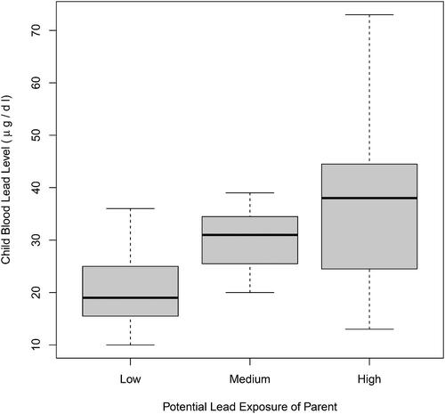
Table 1 Child blood lead levels by parent exposure level.

Exposure level	Child blood lead levels (micrograms per deciliter)	Average	Standard deviation
Low	10, 15, 16, 17, 21, 23, 27, 36	20.62500	8.12294
Medium	20, 22, 29, 31, 34, 35, 39	30.00000	6.92820
High	13, 14, 18, 23, 24, 25, 34, 35, 37, 38, 39, 41, 43, 44, 45, 48, 49, 62, 73	37.10526	15.53453

In this case, using the alternate form, we find$$\begin{array}{c}F=\frac{1}{(g-1) n {\widehat{\sigma }}^2}\sum _{\{(i,j):\mathrm{ }\mathrm{ }i<j\}}{n}_i{n}_j{({\overline{x}}_i-{\overline{x}}_j)}^2\\ =\frac{1}{(g-1) n {\widehat{\sigma }}^2}\{n_L{n}_M{({\overline{x}}_L-{\overline{x}}_M)}^2\\ \hspace{1em}+n_L{n}_H{({\overline{x}}_L-{\overline{x}}_H)}^2+n_M{n}_H{({\overline{x}}_M-{\overline{x}}_H)}^2\}\\ =\frac{1}{(3-1) 34·164.3312}\{8·7·{({\overline{x}}_L-{\overline{x}}_M)}^2+8·19·{({\overline{x}}_L-{\overline{x}}_H)}^2\\ \hspace{1em}+7·19·{({\overline{x}}_M-{\overline{x}}_H)}^2\}\\ =\frac{1}{(3-1) 34·164.3312}\left\{4,921.875+41,283.059+6,714.474\right\}\\ =4.74\end{array}$$

If the necessary assumptions are true, then under the null hypothesis this F statistic follows an F distribution with 2 numerator degrees of freedom and 31 denominator degrees of freedom. This gives a p-value of about 0.016 so, for example, with a significance level of 0.05 we reject the hypothesis of equal mean blood lead levels across the three exposure levels.

Furthermore, using the alternate form we may state what fraction of the F statistic is attached to each of the pairs of samples as shown in Table 2.

Table 2 Contributions to the F statistic by pairs of samples.

Pairs of exposure levels	$n_i{n}_j{({\overline{x}}_i-{\overline{x}}_j)}^2$	Contribution to the F statistic
Low-medium	4921.875	9.3%
Low-high	41,283.059	78.0%
Medium-high	6714.474	12.7%
Total:	52,919.408

2 Kruskal–Wallis Statistic Alternate Form

A similar alternate form may be given for the Kruskal–Wallis test of equal distributions. Here the standard test statistic is$$K=\frac{12}{n(n+1)}\left[\sum _{i=1}^{g_{}}{n}_i{({\overline{R}}_i-(n+1)/2)}^2\right]$$where ${\overline{R}}_i$ is the average rank of the observations from sample i. The rest of the notation is as above. If the null hypothesis is true, then K will follow an approximate ${\chi }_{df}^2$ distribution, with degrees of freedom $df=g-1$. (This approximation is generally considered good with g = 3 groups if the samples sizes are all at least 5, and with g larger than 3 if the sample sizes are all at least 4. See, e.g., Rice 1995).

The average of the assigned ranks $1,2,3,\dots$, n is $(n+1)/2$. Consequently, K is large when there are some average ranks ${\overline{R}}_i$ that are far from the overall average rank of $(n+1)/2$. As with the F statistic above, however, one may compare pairs of average ranks directly in determining the size of the Kruskal–Wallis statistic. Some algebra gives(2) $$\begin{array}{c}K=\frac{12}{n(n+1)}\left[\sum _{i=1}^{g_{}}{n}_i{({\overline{R}}_i-(n+1)/2)}^2\right]\\ =\frac{12}{n(n+1)}\left[\frac{1}{n}\sum _{\left\{(i,j):i<j\right\}}{n}_i{n}_j{({\overline{R}}_i-{\overline{R}}_j)}^2\right]\mathrm{}.\end{array}$$(2)

So, as before, the good news with this alternate form for K is that we can readily see:

1. Large contributions to the K statistic occur when pairs of average ranks are substantially different.

2. In the unbalanced situation (i.e., different sample sizes), the contribution of $n_i{n}_j{({\overline{R}}_i-{\overline{R}}_j)}^2$ to the size of the K statistic depends not only on the difference in average ranks, but also on the product of the sample sizes.

3. $n_i{n}_j{({\overline{R}}_i-{\overline{R}}_j)}^2/\sum n_i{n}_j{({\overline{R}}_i-{\overline{R}}_j)}^2$ is the fraction of the K statistic due to just the difference in samples i and j. This decomposition cannot be seen using the standard K statistic.

In the balanced sample case—say that each sample size $n_i=s$ so that n = gs, note that the K statistic reduces to$$K=\frac{12}{n(n+1)}\frac{s}{g}\left[\sum _{\left\{(i,j):i<j\right\}}{({\overline{R}}_i-{\overline{R}}_j)}^2\right].$$

For the lead example above K can be shown to be 8.51 with an associated p-value of 0.014. (Average ranks were assigned to ties—rank 11.5 for the two values of 23, rank 18.5 for the two values of 34, rank 20.5 for the two values of 35, and rank 25.5 for the two values of 39. For simplicity, no correction term was included for ties.) Consequently, we reject the hypothesis of equal blood lead level distributions across the three exposure levels at the 0.05 level.

For the K statistic it can be shown, using 3. above, that 10.4% is due to the difference in the Low and Medium exposure groups, 11.0% is due to the difference in the Medium and High exposure groups, and 78.6% is due to the difference in the Low and High exposure groups.

3 Closing Comment

The various alternate forms of the one-way ANOVA F statistic and the Kruskal–Wallis statistic are scarce in the balanced sample case and possibly non-existent in the unbalanced sample case within the statistical literature. However, these alternate forms are similar in spirit to a result concerning the computation of the sample variance which does have some visibility in the statistical literature. In particular, given data values $x_1,x_2,\dots ,x_n$, the sample variance may be written without reference to the sample mean:$$s^2=\frac{1}{n-1}\sum _{i=1}^n{(x_i-\overline{x})}^2=\frac{1}{(n-1)n}\sum _{\{(i,j):i<j\}}{(x_i-x_j)}^2.$$

This result may be found, for example, in Heffernan (1988), and even appeared on the cover of the journal Teaching Statistics in 2009 (vol. 31, no. 2).

Supplementary Materials

In the supplement, we provide exercises for students to investigate the alternate forms of the one-way ANOVA F and Kruskal-Wallis test statistics. Notes for instructors on these exercises are also provided.

References

- Casella, G., and Berger, R. L. (2002), Statistical Inference, 2nd ed., Pacific Grove, CA: Duxbury.
- Centers for Disease Control (2021), “Health Effects of Lead Exposure,” https://www.cdc.gov/nceh/lead/prevention/health-effects.htm, Accessed 4 September 2021.
- Heffernan, P. (1988), “New Measures of Spread and a Simpler Formula for the Normal Distribution,” The American Statistician, 42, 100–102.
- Morton, D. E., Saah, A. J., Silberg, S. L., Owens, W. L., Roberts, M. A., and Saah, M. D. (1982), “Lead Absorption in Children of Employees in a Lead-Related Industry,” American Journal of Epidemiology, 115, 549–555.
- Rice, J. (1995), Mathematical Statistics and Data Analysis, 2nd ed., Belmont, CA: Duxbury Press, p. 454.