Regression, Transformations, and Mixed-Effects with Marine Bryozoans

Abstract

This article demonstrates how data from a biology paper, which analyzes the relationship between mass and metabolic rate for two species of marine bryozoan, can be used to teach a variety of regression topics to both introductory and advanced students. A thorough analysis requires intelligent data wrangling, variable transformations, and accounting for correlation between observations. The bryozoan data can be used as a valuable class example throughout the semester, or as a dataset for extended homework assignments and class projects. Supplementary materials for this article are available online.

Keywords:

• Applications
• Correlated data
• Data processing
• Regression assumptions

1 Introduction

From an evolutionary perspective, an individual organism’s success is judged by its ability to reproduce, and the most successful organisms are those which make the biggest contribution to their species’ gene pool. In many species, one factor associated with reproductive success is size, but there are competing explanations for this association. In Pettersen, White, and Marshall (2015), the authors propose that larger organisms, though they use a greater amount of energy than smaller organisms, are more energy efficient proportional to their body size.

To investigate, the authors collected data on two species of marine bryozoan, Bugula neritina and Watersipora subtorquata. The mass and metabolic rate of these individuals were recorded, and regression was used to model the relationship between mass and metabolic rate. While linear regression on the raw data can assess the first component of the researchers’ hypothesis (larger organisms use more energy), a linear relationship is not appropriate to assess the second component (larger organisms are more energy efficient, proportional to body size). The authors therefore, apply a log transformation to both mass and metabolic rate; linear regression on the log-log scale can model a wider range of relationships on the untransformed scale, and whether larger organisms are more energy efficient corresponds to whether the slope of the line is less than 1 on the log-log scale (Pettersen, White, and Marshall 2015).

The purpose of this article is to show how the research paper, marine bryozoan data, and research questions from Pettersen, White, and Marshall (2015) are a valuable tool for teaching students about data analysis and regression. For students in a first- or second-semester statistics course, I have used these data in labs, assignments, and projects to teach students about data wrangling, transformations, and regression assumptions. For more advanced students, these data provide a good example of repeated measures and mixed-effects models. There are several aspects of the marine bryozoan data that make it particularly valuable in the classroom:

• The original article can be used to teach students how to read a research paper and focus on the motivation and statistical analysis.

• A simplified version of the analysis conducted by Pettersen, White, and Marshall (2015) can be performed with students in first- or second-semester courses, which allows them not only to apply the tools they learn to real data, but also to see how those tools are used by researchers in real studies.

• Unlike many examples of variable transformations at the introductory level, the log transformations are needed to actually answer the research question, rather than to fix violations of the linear regression assumptions.

• On the log-log scale, we are interested in whether the slope is less than 1. This allows students to see an example where the specific value of the slope is of interest, rather than just whether it is 0.

• As with many scientific studies, data were collected over multiple experimental runs, with noticeable variation between runs. A standard approach to account for this additional variability in the model is to include experimental run as a random effect, as the authors of the original paper do (Pettersen, White, and Marshall 2015). For more advanced students, these data provide a natural example for teaching mixed-effects models.

• The data collection includes repeated measures on the same individuals at different stages of their life. Introductory students can practice identifying this violation of the independence assumption for linear regression. For students in more advanced courses, this dependence can be accounted for by adding additional random effect terms to the model, or with repeated-measures hypothesis testing.

• Repeated measures and multiple runs in the study design give the data an interesting structure. This structure is valuable for teaching students data wrangling and exploratory data analysis.

1.1 Data and Code

The original data discussed in this article were made available by Pettersen, White, and Marshall (2015) on Dryad (https://perma.cc/26ZZ-CSK9) under a CC0 1.0 Universal (CC0 1.0) Public Domain Dedication license. The raw data can be found at https://github.com/ciaran-evans/bryozoan-data-paper, along with a script for cleaning, fixing the errors discussed in Section 4.2, and performing the analyses contained in this article. For instructors who want to focus on modeling rather than data wrangling, the fully cleaned and corrected data are available in the same repository. The same material found in the GitHub repository can also be found in the supplementary materials for this article.

The data processing and modeling code provided is in R (R Core Team 2021), which is the statistical computing language used in my classes. I find that the tidyr (Wickham 2021), dplyr (Wickham et al. 2021), and ggplot2 (Wickham 2016) packages allow students to do extensive data cleaning and visualization with a small number of functions, and the lme4 package (Bates et al. 2015) is great for fitting mixed models. However, the activities discussed below are language-independent, and the same analysis could be done with other software.

2 Reading a Research Paper

Before giving students the bryozoan data for exploratory data analysis and modeling, it can be valuable for them to read and summarize the original biology paper. This provides further background information on the study and its motivation, teaches important skills for engaging with original research, and can be used to frame later activities that will attempt to reproduce the results of the original analysis.

I recommend that students read the paper several times, focusing on different aspects with each reading. On the first read through, they should concentrate on the overall motivation for the research, and summarizing the data and statistical methods used for analysis. Subsequent readings can focus on identifying specific details, like the modeling choices made by the authors (e.g., which variables were included in the model, and were any interaction terms included). To guide students through their first reading, I have created an activity that introduces the research paper, summarizes the sections of a journal article, and suggests which paragraphs the students should focus on. The activity is available on my website (https://ciaran-evans.github.io/files/bryozoan_paper_activity.html), and the original R Markdown file can be found in the GitHub repository for this paper (https://github.com/ciaran-evans/bryozoan-data-paper).

This activity can be assigned either for homework or as an extended in-class exercise. If given in class, I recommend allowing most of the class period for students to complete and discuss the questions. Working in groups of 2–3, students can read the Introduction together, then divide the remaining sections between them.

POTENTIAL PITFALL: Even with scaffolded questions that walk through the research paper, introductory students may struggle to identify key information in a journal article. Before assigning the research paper as a class activity or homework assignment, I recommend introducing the data, research question, and learning goals in class.

3 Data

Data were collected by Pettersen, White, and Marshall (2015), with B. neritina and W. subtorquata sampled at two yacht clubs in Victoria, Australia. After initial growth, the developmental process of these two species consists of three phases before they are considered mature—a larval stage (before the individual settles and begins metamorphosis), an early post-settlement stage, and a late post-settlement stage (as the individual nears the end of metamorphosis). Researchers collected larvae from their sampled B. neritina and W. subtorquata, and tracked these offspring from the larval through late post-settlement stages.

For each individual offspring, the researchers measured the mass (in micrograms, μg) and the metabolic rate (the rate at which energy is consumed, in millijoules per hour, mJ/hour).

POTENTIAL PITFALL:

Students often think that having a “fast metabolism” is a good thing. Remind them that a larger metabolic rate simply means that the organism uses more energy.

Measurements were taken over 21 different runs (repetitions of the experiment), with a different set of individuals for each run. Due to experimental constraints, individuals measured at the larval stage could not later be measured at the early and late post-settlement stages. Each run therefore, consisted of two groups of individuals: larvae and settlers. The larvae were measured at the beginning of the run (before maturing further), and the settlers were measured at two different time points: at the beginning of the run (early post-settlement stage) and at the end (late post-settlement stage). This means that the same individuals are measured at the early and late stages, but different individuals are measured at the larval stage.

HELPFUL HINT:

For introductory classes where experimental run cannot be accounted for in the model, I gloss over or ignore this variable in the data.

The resulting dataset contains 823 rows, with columns for Species, Run, Stage, Mass (μg), and Metabolic Rate (mJ/hour). There are no missing observations.

HELPFUL HINT:

Students are likely unfamiliar with marine bryozoans, but fortunately mass and metabolism are familiar concepts. When using these data in class, it is important to provide background information on the data, and to emphasize (1) the familiar variables, and (2) the structure of the data.

TEACHING TIP:

When using this data for a class project, it can be helpful for the instructor to play the role of the “client,” who can answer any questions the students have about the data but isn’t sure what statistical methods to use.

4 Exploratory Data Analysis and Data Preparation

4.1 How Many Individual Organisms are in the Data?

Students often think about data without repeated measurements, so each observation corresponds to a different individual (or country, or company, etc.). However, the bryozoan data has repeated measurements on the early and late stage individuals, so while there are 823 rows, there are not 823 different individuals. Asking students to calculate the number of different individuals is a good way for them to get familiar with the structure of the bryozoan data, and is good practice with basic data wrangling.

The answer (568 different individuals) can be arrived at by simply removing the late stage rows (e.g., with filter or subset in R), but requires students to recognize that different individuals are measured at the larval and early/late stages. For more involved data wrangling, students can also be asked to check that the same number of individuals is recorded in the early and late stages within each run.

4.2 Measurements of Mass and Metabolic Rate, and Potential Errors in the Data

From the study description, we know that the researchers measured the settlers at two different time points: the early and late post-settlement stages. Were both mass and metabolic rate measured at each time point, or just one of the variables? Careful examination of the W. subtorquata rows in the bryozoan data shows that within a run, the early and late-stage measurements have the same masses, but not the same metabolic rates. This suggests that mass was measured once for the early/late stages, but metabolic rate was measured at each time point.

TEACHING TIP:

Efficiently checking whether mass and metabolic rate are measured once or twice requires students to think outside the box and creatively put together a few different data wrangling tools. In R, one way this can be accomplished is with the filter and full_join functions in the dplyr package; full details can be found in the code at https://github.com/ciaran-evans/bryozoan-data-paper.

For the B. neritina portion of the data, the story is a little different. Applying the same approach as for the W. subtorquata rows initially suggests that both mass and metabolic rate are measured twice. But if we compare the distributions of mass across different stages, we notice that the mass for the late-stage Bugula is very different from mass for the larval and early stages (Figure 1). Furthermore, the distribution of mass for late-stage Bugula looks suspiciously like the distribution of metabolic rate for early-stage Bugula!

Fig. 1 Distributions of bryozoan mass and metabolic rate by species and stage, in the original (uncorrected) data.

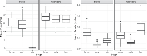
As it turns out, the original data file has an error, in which metabolic rates for early-stage Bugula appear again as masses for late-stage Bugula (the error has since been corrected by the authors, but I prefer to keep the error for teaching students about data cleaning). Under the assumption that the researchers measured mass once (as for the Watersipora), we can correct the data by replacing the late-stage Bugula masses with the early-stage Bugula masses. For the rest of this article, we will use the corrected data. (Thinking about the structure of the data, in which mass is the same for early and late post-settlement stages, we can even speculate on how the error occurred: a researcher may have intended to copy the early-stage masses, and accidentally copied the early-stage metabolic rates).

TEACHING TIP:

For advanced students, see if they can find the issue on their own. Students examining Figure 1 should be curious about the strange distribution of mass for late-stage Bugula, and a little more data sleuthing reveals the error.

4.3 Multivariate EDA

We’ve already seen in Figure 1 that the distributions of mass and metabolic rate appear to differ between species and stage. The relationship between mass and metabolic rate also seems to vary across species and stages, as shown in Figure 2. This suggests that any model should either account for species and stage, or should be fit only on a subset of the data.

Fig. 2 Relationship between mass and metabolic rate for marine bryozoans by species and stage, in the corrected data.

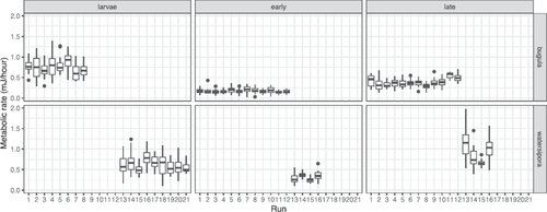
For more advanced students, we can also think about experimental variability between different runs, and Figure 3 shows between-run variability. This is often called technical variability, and is commonly accounted for by random effects terms in the model. We discuss a mixed-effects model for the bryozoan data in Section 8.

Fig. 3 Distribution of metabolic rate for each run in the study, by species and stage.

5 Simple Linear Regression

5.1 Subsetting the Data

As shown in Figure 2, differences between species and stages mean that if we want to fit a simple linear regression model, we should focus only on a subset of the data. For this Section and Section 6, we will use only early-stage Bugula, but other species-stage combinations are possible. After restricting the data to the early-stage Bugula, we have 197 rows, each corresponding to a different organism.

5.2 Fitting a Model

Do larger early-stage Bugula tend to have a higher metabolic rate? This is what we expect, since from our own experience we know that larger organisms require more food—for example, your daily recommended calorie intake depends on factors like weight and height. To explore this question, we fit a linear regression of metabolic rate on mass:(1) $$\text{metabolic}\mathrm{ }\text{rate}={\beta }_0+{\beta }_1\text{mass}+\epsilon .$$(1)

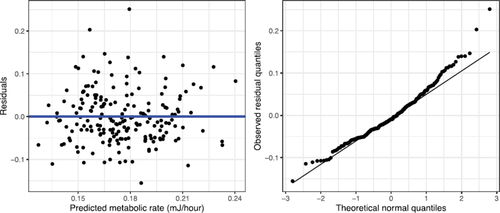
The equation of the fitted line is $\widehat{\text{metabolic}\mathrm{ }\text{rate}}=0.0831+0.0064\text{mass}$, with the positive slope suggesting that larger organisms do require more energy. Regression diagnostics look pretty reasonable, with no clear violations of the linearity or constant variance assumptions (Figure 4). The distribution of the residuals looks a little nonnormal, but with 197 early-stage Bugula for our simple linear regression, we’re not concerned about some departures from normality.

Fig. 4 Residual and normal QQ plots for linear regression of metabolic rate on mass in the early-stage Bugula.

TEACHING TIP:

Ask students to assess the assumption of independence, and ask whether their answer would change if we fit the model on the full data (which has repeated measurements) rather than just the early-stage Bugula. In introductory classes I often ignore the Run variable in the dataset, so students identify that the independence assumption is reasonable for the early-stage Bugula but not for the full data. In advanced classes, students should recognize that Run is still a source of correlation between observations (which we account for with random effects in Section 8).

We are 95% confident that an increase of 1μg in mass is associated with an increase in metabolic rate of between 0.0038 mJ/hour and 0.0090 mJ/hour. Furthermore, the p-value for the t-test of the hypotheses $H_0:{\beta }_1=0$ versus $H_A:{\beta }_1>0$ is $8.15\times {10}^{-7}$, so we have strong evidence that larger early-stage Bugula do indeed require more energy, as expected.

6 Log Transformations

A positive relationship between mass and metabolism is only the first part of the researchers’ hypothesis. The second part is that, proportional to body size, larger individuals are more energy efficient. The next step is for students to recognize that the linear regression model in (1) is inappropriate for assessing this hypothesis.

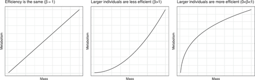
Advanced students can be asked to explain why the linear model in (1) is inappropriate, and to sketch a relationship which supports the researchers’ hypothesis. With introductory students, I ask them to interpret the slope β₁ from (1): an increase of 1 μg in mass is associated with a change of β₁ mJ/hour in metabolic rate, on average. Students then realize that this interpretation does not depend on the value of mass, as the slope is the same for all values of mass. If the researchers’ hypothesis is correct, however, we would expect that the slope (the metabolic penalty for an increase in size) decreases for larger organisms. The three possibilities for size and energy efficiency can be summarized with the curves in Figure 5.

Fig. 5 Possible relationship shapes between mass and metabolism, using the model in (2).

POTENTIAL PITFALL:

Students who confuse the true (unknown) relationship with the model we choose (our approximation of the true relationship, which may be good or bad) will be confused why (1) is “wrong,” especially since the linearity and constant variance assumptions looked reasonable in Figure 4.

To capture these different possibilities, Pettersen, White, and Marshall (2015) propose that(2) $$\text{metabolic}\mathrm{ }\text{rate}\approx \alpha {\text{mass}}^{\beta },$$(2) where α and β are unknown parameters. The value of β corresponds to the curvature of the relationship, as shown in Figure 5. Therefore, the hypothesis that larger organisms are more energy efficient corresponds to $\beta <1$.

TEACHING TIP:

For students of sufficient mathematical maturity, the interpretation of β as the percent change in metabolic rate associated with a 1% change in mass may be useful.

How do we fit this model? Advanced students can be asked to propose a transformation that allows the model to be fit with linear regression. For introductory students, I show them that a log-transform of both sides yields(3) $$\text{log}\hspace{0.17em}(\text{metabolic}\mathrm{ }\text{rate})\approx \hspace{0.17em}\text{log}\hspace{0.17em}\alpha +\beta \hspace{0.17em}\text{log}\hspace{0.17em}\text{mass}$$(3)

By rewriting ${\beta }_0=\hspace{0.17em}\text{log}\hspace{0.17em}\alpha$ and ${\beta }_1=\beta$, then we have a linear relationship between the transformed variables (log metabolic rate and log mass)! To summarize, the transformed linear model is(4) $$\text{log}\hspace{0.17em}(\text{metabolic}\mathrm{ }\text{rate})={\beta }_0+{\beta }_1\hspace{0.17em}\text{log}\hspace{0.17em}\text{mass}+\epsilon .$$(4)

POTENTIAL PITFALL:

Students often forget how to work with logs. A reminder of basic properties is useful, otherwise the transformations will be confusing.

HELPFUL HINT:

I do not use this example as the first introduction to transformations, because the transformation isn’t necessary to make the data look roughly linear. Students should have seen transformations for clearly nonlinear data before (e.g., a log transformation on the Gapminder data Bryan 2017).

TEACHING TIP:

This discussion provides an example where the shape of our model is not chosen solely from the data.

TEACHING TIP:

Regression on the log-log scale is also common in measuring elasticity between economic variables in microeconomics. An absolute slope less than 1 on the log-log scale indicates that the response has an inelastic relationship with the predictor, while an absolute slope greater than 1 indicates an elastic relationship. This connection may provide useful intuition for students who have taken economics courses.

Students then transform both mass and metabolic rate, and fit the model in (4). The equation of the fitted model (on the early-stage Bugula) is $\widehat{\hspace{0.17em}\text{log}\hspace{0.17em}(\text{metabolic}\mathrm{ }\text{rate})}=-3.40+0.60\hspace{0.17em}\text{log}\hspace{0.17em}(\text{mass})$.

TEACHING TIP:

Ask students to transform the predictions back to the original scale of the data and plot the predictions (on the original scale) on a scatterplot of mass and metabolic rate, so they can see that fitting a linear regression on the log-log scale corresponds to fitting a curve on the raw scale.

POTENTIAL PITFALL:

If the model is fit on the combined data, without subsetting or including species and stage as covariates, then the estimated slope is actually > 1! (This could also serve as an example of Simpson’s paradox). When using these data for simple linear regression, it is important to use only one species and stage at a time.

Because the slope of the fitted line is between 0 and 1, our estimated regression model supports the hypothesis that larger organisms are more energy efficient, proportional to body size. Diagnostics, particularly the residual plot, look similar to Figure 4 above. We are 95% confident that the true change in log metabolic rate associated with a unit increase in log mass is between 0.37 and 0.83 (or equivalently that a 1% increase in mass is associated with between a 0.37% and a 0.83% increase in metabolic rate).

What about a hypothesis test? Because the researchers hypothesize that larger organisms are more energy efficient, proportional to body size, then the correct hypotheses are $H_0:{\beta }_1=1$ versus $H_A:{\beta }_1<1$.

TEACHING TIP:

This serves as a nice example where we really care about testing a value other than 0 for the slope. Similar examples can be found in other literature on body mass and metabolic rate, for example, Kleiber (1947), who suggests a slope of 0.75 on the log-log scale.

The test statistic is $t=-3.45$, and the p-value is 0.00034, so we have strong evidence that larger early-stage Bugula are more energy efficient, proportional to body size, than smaller early-stage Bugula.

POTENTIAL PITFALL:

Students who are accustomed to simply reading off the p-value from a summary of regression output (e.g., the summary function in R) will not realize that this p-value tests the wrong hypotheses (${\beta }_1=0$ vs. ${\beta }_1\ne 0$).

7 Multiple Linear Regression

Of course, the researchers are not just interested in early-stage Bugula. They would like to fit a multiple regression model for multiple species and stages. What model is appropriate? Due to dependence between the early and late stages, it is inappropriate to include both in the model without accounting for repeated measures. On the other hand, different organisms were measured at the larval stage, without repeated measures. In Pettersen, White, and Marshall (2015), the researchers decided to combine the larval and early-stage measurements in one model, but exclude the late-stage measurements to avoid dependence.

As shown in Figure 6, it certainly appears important to include both Species and Stage in the model for log metabolic rate. Furthermore, students should recognize that an interaction between Species and Stage is likely required. Without an interaction, the vertical distance between the larval and early-stage lines would be the same for both Bugula and Watersipora, but the vertical distances appear different in Figure 6.

Fig. 6 Relationship between log mass and log metabolic rate for larval and early-stage bryozoans.

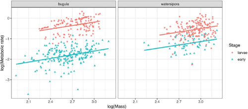
TEACHING TIP:

Interactions can be a difficult concept for students. To motivate the need for an interaction term from Figure 6, ask students to consider the additive model$$\begin{array}{c}\hspace{0.17em}\text{log}\hspace{0.17em}(\text{metabolic}\mathrm{ }\text{rate})={\beta }_0+{\beta }_1\text{Watersipora}+{\beta }_2\text{Early}\\ \hspace{1em}+{\beta }_3\hspace{0.17em}\text{log}\hspace{0.17em}(\text{mass})+\epsilon ,\end{array}$$and sketch what the fitted lines would look like with various combinations of$$\text{Watersipora}=\{\begin{array}{cc}1\hfill & \text{species}\mathrm{ }\text{is}\mathrm{ }\text{Watersipora}\hfill \\ 0\hfill & \text{otherwise}\hfill \end{array}$$

and$$\text{Early}=\{\begin{array}{cc}1\hfill & \text{early}\mathrm{ }\text{post}-\text{settlement}\mathrm{ }\text{stage}\hfill \\ 0\hfill & \text{otherwise}\hfill \end{array}$$in the additive model.

The slopes for each species and stage, however, look pretty similar. A reasonable first model would then be(5) $$\begin{array}{c}\hspace{0.17em}\text{log}\hspace{0.17em}(\text{metabolic}\mathrm{ }\text{rate})={\beta }_0+{\beta }_1\text{Watersipora}+{\beta }_2\text{Early}\\ \hspace{1em}+{\beta }_3\text{Watersipora}·\text{Early}\\ \hspace{1em}+{\beta }_4\hspace{0.17em}\text{log}\hspace{0.17em}(\text{mass})+\epsilon ,\end{array}$$(5) and the equation of the fitted model is(6) $$\begin{array}{c}\widehat{\hspace{0.17em}\text{log}\hspace{0.17em}(\text{metabolic}\mathrm{ }\text{rate})}=-1.92-0.32\text{Watersipora}-1.42\text{Early}\\ \hspace{1em}+0.79\text{Watersipora}·\text{Early}\\ \hspace{1em}+0.58\hspace{0.17em}\text{log}\hspace{0.17em}(\text{mass}).\end{array}$$(6)

The adjusted coefficient of determination is $R_{\text{adj}}^2=0.77$. The interaction term in (5) is significant, with a p-value of essentially 0, and the adjusted coefficient of determination without the interaction term drops to $R_{\text{adj}}^2=0.71$. As in the simple linear regression model in Section 6, the estimated coefficient on log mass, 0.58, is between 0 and 1. The corresponding 95% confidence interval is [0.43, 0.72], and a t-test of $H_0:{\beta }_4=1$ versus $H_A:{\beta }_4<1$ (with β₄ in (5)) gives a p-value of about $5.7\times {10}^{-9}$. This supports the hypothesis that larger bryozoans are more energy efficient, proportional to body size, than smaller bryozoans.

Of course, in our model in (5) we have assumed that the slope is the same regardless of species and stage. Does the slope differ between species or stages? To assess this question, we compare the (reduced) model in (5) with a (full) model containing all possible interaction terms. For the complete interaction model, $R_{\text{adj}}^2=0.76$, so adding additional interaction terms does not help explain variability in log metabolic rate. A nested F-test can be used to compare the two models; the p-value is 0.993, suggesting there is very little evidence for a difference in slope between Species or Stages.

TEACHING TIP:

Students are often fuzzy about the difference between t-tests and nested F-tests, particularly as a t-test of $H_0:{\beta }_i=0$ versus $H_A:{\beta }_i\ne 0$ is equivalent to a nested F-test. Ask the students to explain why a nested F-test was not appropriate for our previous hypothesis test, comparing $H_0:{\beta }_4=1$ and $H_A:{\beta }_4<1$.

8 Mixed-Effects Models

While multiple regression in the previous section allowed us to investigate the research question for multiple species and stages, we have failed to capture a source of dependence and variability in the larval and early-stage bryozoans: experimental Run. As we saw in Figure 3, there is substantial variability between runs, suggesting that we may need to include this variable in the model. Much of the notation and model-building process for mixed-effects models in this section is based on Chap. 8 of Roback and Legler (2021), which is a valuable resource for teaching mixed-effects models to intermediate and advanced undergraduates.

When first asked to consider including Run, students may want to use Run as a fixed effect, with a different intercept for each run. However, viewing each Run as a random draw from all possible experimental runs, and not wanting to add 20 more parameters to our model, it makes more sense to include Run as a random effect.

TEACHING TIP:

To motivate the use of a random effect here, it could help to ask students the simple question “Do we care about comparisons between specific runs?” The answer is no, so a random effect is useful for Run. On the other hand, we do care about comparisons between species and stages (and the species and stages under consideration were fixed by the study design), so we should use fixed effects for Species and Stage.

To further examine variability between the different runs, we begin with a simple random intercepts model:(7) $$\text{log}\hspace{0.17em}{(\text{metabolic}\mathrm{ }\text{rate})}_{ij}={\beta }_0+u_i+{\epsilon }_{ij},$$(7) where $\text{log}\hspace{0.17em}{(\text{metabolic}\mathrm{ }\text{rate})}_{ij}$ is the log metabolic rate for observation j in run i, and $u_i\sim N(0,{\sigma }_u^2)$ and ${\epsilon }_{ij}\sim N(0,{\sigma }_{\epsilon }^2)$.

TEACHING TIP:

The simple random intercept model in (7) is analogous to the one-way ANOVA model we would get by treating Run as a fixed effect.

Fitting (7) with restricted maximum likelihood estimation gives ${\widehat{\sigma }}_u^2=0.18$ and ${\widehat{\sigma }}_{\epsilon }^2=0.43$ (the results are very similar for maximum likelihood estimation). This gives an intraclass correlation coefficient of 0.3, so observations from the same run are moderately correlated. Testing whether there are differences across runs is a test for the variance parameter ${\sigma }_u^2$, with the null and alternative hypotheses $H_0:{\sigma }_u^2=0$ versus $H_A:{\sigma }_u^2>0$.

POTENTIAL PITFALL:

Students used to fixed effects may expect that all hypotheses are about parameters β_i in the regression model, not realizing that the variance parameter ${\sigma }_u^2$ is also part of our model.

Different methods can be used to test these hypotheses. The simplest is a likelihood ratio test to compare the model in (7) with a reduced model that drops the random effect term; this can be performed with the anova function in R, though the resulting p-value is conservative since ${\sigma }_u^2=0$ is at the edge of the parameter space (see, e.g., Self and Liang 1987). Another option is to use a simulation-based likelihood ratio test (Scheipl, Greven, and Kuechenhoff 2008), implemented in R in the RLRsim package. In this case, the p-value is essentially 0 regardless of the procedure employed—possibly because other covariates, like species and stage, need to be included in the model.

HELPFUL HINT:

Hypothesis testing with mixed-effects models can be challenging. Ben Bolker has put together a very useful summary of discussion on this topic, and other aspects of (G)LMMs: https://perma.cc/T86L-KY2A.

We then extend our multiple regression model (5) to include a random intercept for each run:(8) $$\begin{array}{c}\hspace{0.17em}\text{log}\hspace{0.17em}{(\text{metabolic}\mathrm{ }\text{rate})}_{ij}={\beta }_0+u_i+{\beta }_1{\text{Watersipora}}_{ij}+{\beta }_2{\text{Early}}_{ij}\\ \hspace{1em}+{\beta }_3{\text{Watersipora}}_{ij}·{\text{Early}}_{ij}\\ \hspace{1em}+{\beta }_4\hspace{0.17em}\text{log}\hspace{0.17em}{(\text{mass})}_{ij}+{\epsilon }_{ij}.\end{array}$$(8)

Fitting the model in (8) gives ${\widehat{\beta }}_4=0.68$, which still supports the researchers’ hypothesis that larger organisms are more energy efficient, proportional to body size. The estimated random effect variance is ${\widehat{\sigma }}_u^2=0.012$, and a test of $H_0:{\sigma }_u^2=0$ versus $H_A:{\sigma }_u^2>0$ again yields a p-value of essentially 0. The estimated error variance is ${\widehat{\sigma }}_{\epsilon }^2=0.12$, which is a 72% decrease from the simple random effects model (7) after adding in the fixed effects.

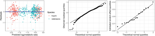
Figure 7 suggests that the model assumptions for (8), including the assumption that the random effects u_i are normal, are reasonable. As in previous sections, our primary research question is whether larger organisms are more energy-efficient, proportional to body size, which corresponds to the hypotheses $H_0:{\beta }_4=1$ versus $H_A:{\beta }_4<1$ for the model in (8). The simplest method is with a t-test, which gives a test statistic of $t=-4.37$. This is a pretty extreme test statistic, but if we insist on computing a p-value we can use an approximation for the degrees of freedom, such as Satterthwaite or Kenward-Rogers (Halekoh and Højsgaard 2014; Kuznetsova, Brockhoff, and Christensen 2017). Using the t-distribution, a 95% confidence interval for the true slope β₄ is [0.531, 0.822]. For mixed-effects models, a parametric bootstrap is often more appropriate, though in this case a simple 95% parametric bootstrap percentile interval with 10,000 repetitions is essentially the same, [0.532, 0.821].

Fig. 7 Diagnostic plots for the fitted model (8). The middle plot shows a normal quantile-quantile plot for the residuals ${\widehat{\epsilon }}_{ij}$, while the plot on the right is a normal quantile-quantile plot for the estimated random effects ${\widehat{u}}_i$ for each run i.

TEACHING TIP:

Getting the degrees of freedom “right” for the hypothesis test in this case isn’t particularly interesting. The p-value summarizes the strength of evidence against H₀, and a test statistic of $t=-4.37$ is strong evidence regardless of how we approximate the degrees of freedom.

TEACHING TIP:

Software sometimes includes functions that automatically perform bootstraps (e.g., the bootMer function in the lme4 R package (Bates et al. 2015) is very useful for parametric bootstrapping), but writing your own parametric bootstrap function can be a valuable assignment for advanced students.

However, the model in (8) assumes that the slope on log mass is the same for each run, when in reality the slope may vary between runs. We can add a random slope for each run as well:(9) $$\begin{array}{c}\hspace{0.17em}\text{log}\hspace{0.17em}{(\text{metabolic}\mathrm{ }\text{rate})}_{ij}={\beta }_0+u_i+{\beta }_1{\text{Watersipora}}_{ij}+{\beta }_2{\text{Early}}_{ij}\\ \hspace{1em}+{\beta }_3{\text{Watersipora}}_{ij}·{\text{Early}}_{ij}\\ \hspace{1em}+({\beta }_4+v_i)\hspace{0.17em}\text{log}\hspace{0.17em}{(\text{mass})}_{ij}+{\epsilon }_{ij},\end{array}$$(9)

with noise ${\epsilon }_{ij}\sim N(0,{\sigma }_{\epsilon }^2)$ and random effects(10) $$\left[\begin{array}{c}{u}_i\\ v_i\end{array}\right]\sim N\left(\left[\begin{array}{c}0\\ 0\end{array}\right],\left[\begin{array}{cc}{\sigma }_u^2& \rho {\sigma }_u{\sigma }_v\\ \rho {\sigma }_u{\sigma }_v& {\sigma }_v^2\end{array}\right]\right).$$(10)

The interpretation of the fixed effect slope β₄ in (9) is now slightly different: β₄ is now the average slope across runs in the population. Inference for β₄ is still of interest to address the research question: ${\widehat{\beta }}_4=0.67$, and a 95% parametric bootstrap confidence interval for β₄ is [0.510, 0.830]. Estimates for the other coefficients are shown in Table 1. For the random effects, ${\widehat{\sigma }}_u^2=0.15$, ${\widehat{\sigma }}_v^2=0.017$, and $\widehat{\rho }=-0.96$.

Table 1 Estimated coefficients for fixed effects in (9).

	Estimate	Standard error	t-value
Intercept	–2.18	0.23	–9.68
Watersipora	–0.34	0.07	–5.12
Early	–1.42	0.04	–34.17
Watersipora $·$ Early	0.76	0.07	10.71
log(mass)	0.67	0.08	8.38

Once again, we have reached the conclusion that larger organisms are more energy efficient, proportional to body size. While it turns out that including Run as a random effect didn’t change that conclusion, we have seen that there is substantial variability between runs, and including it in the model captures that additional source of variability.

9 Conclusion

The bryozoan data can be used in a wide range of statistics and data science courses, to teach topics ranging from data wrangling and preparation, to regression and transformations, to mixed-effects models. A thorough analysis requires students to synthesize several of these skills, which makes the dataset particularly useful for extended homework assignments and class projects. The data is also useful as an in-class example, which can be referred to throughout the semester to discuss each new concept.

Analysis of these data is not restricted to the examples contained in this article. For example, the mixed-effects model in (9) uses random effects to account for correlation between observations within each run, but compares only larval and early-stage bryozoans. Including the late-stage organisms as well requires us to account for the repeated measures on the early- and late-stage bryozoans; this could be done with additional random effects for each individual organism, or through repeated-measures hypothesis testing (the latter option was used by Pettersen, White, and Marshall 2015).

Acknowledgments

Thank you to Gordon Weinberg, Philipp Burckhardt, and Alex Reinhart for discussions on these data and their use in statistics classes. Thank you to Samantha Morrison for discussions on repeated measures and mixed-effects models. Finally, thank you to several anonymous reviewers, the associate editor, and the editor for helpful feedback that improved this manuscript.

Supplementary Materials

The supplementary materials include the raw and corrected bryozoan data, the research paper activity, and all code used for the analysis discussed in this paper.

References

- Bates, D., Mächler, M., Bolker, B., and Walker, S. (2015), “Fitting Linear Mixed-Effects Models using lme4,” Journal of Statistical Software, 67, 1–48. DOI: https://doi.org/10.18637/jss.v067.i01.
- Bryan, J. (2017), gapminder: Data from Gapminder, R package version 0.3.0.
- Halekoh, U., and Højsgaard, S. (2014), “A Kenward–Roger Approximation and Parametric Bootstrap Methods for Tests in Linear Mixed Models—The R Package pbkrtest,” Journal of Statistical Software, 59, 1–30.
- Kleiber, M. (1947), “Body Size and Metabolic Rate,” Physiological Reviews, 27, 511–541. DOI: https://doi.org/10.1152/physrev.1947.27.4.511.
- Kuznetsova, A., Brockhoff, P. B., and Christensen, R. H. B. (2017), “lmerTest package: Tests in Linear Mixed Effects Models,” Journal of Statistical Software, 82(13):1–26. DOI: https://doi.org/10.18637/jss.v082.i13.
- Pettersen, A. K., White, C. R., and Marshall, D. J. (2015), “Why does Offspring Size Affect Performance? Integrating Metabolic Scaling with Life-History Theory,” Proceedings of the Royal Society B: Biological Sciences, 282, 20151946. DOI: https://doi.org/10.1098/rspb.2015.1946.
- R Core Team (2021), R: A Language and Environment for Statistical Computing, Vienna, Austria: R Foundation for Statistical Computing.
- Roback, P., and Legler, J. (2021), Beyond Multiple Linear Regression: Applied Generalized Linear Models and Multilevel Models in R, Boca Raton, FL: CRC Press.
- Scheipl, F., Greven, S., and Kuechenhoff, H. (2008), “Size and Power of Tests for a Zero Random Effect Variance or Polynomial Regression in Additive and Linear Mixed Models,” Computational Statistics & Data Analysis, 52, 3283–3299.
- Self, S. G., and Liang, K.-Y. (1987), “Asymptotic Properties of Maximum Likelihood Estimators and Likelihood Ratio Tests Under Nonstandard Conditions,” Journal of the American Statistical Association, 82, 605–610. DOI: https://doi.org/10.1080/01621459.1987.10478472.
- Wickham, H. (2016), ggplot2: Elegant Graphics for Data Analysis, New York: Springer-Verlag.
- Wickham, H. (2021), tidyr: Tidy Messy Data, R package version 1.1.3.
- Wickham, H., François, R., Henry, L., and Müller, K. (2021), dplyr: A Grammar of Data Manipulation, R package version 1.0.7.