Leveraging the “Large” in Large Lecture Statistics Classes

Abstract

Being a teacher or a student in a class with a large enrollment can be intimidating. Often, teachers view comforts that are common to small classes as unattainable in a larger class, including knowing students’ names, using active learning, employing group work, and creating group discussion. Students in large classes may find that the class size leads to isolation. At Utah State University, we offer introductory statistics classes for various audiences using a large lecture format. The authors have collectively led these large lectures dozens of times and found that, despite its shortcomings, the large lecture format can be an asset when teaching statistics. With an active learning approach such as recommended by the revised GAISE College report, large class sizes permit realistic sampling, facilitate student-driven simulation, and provide bountiful opportunities for experimentation. In this article, we discuss the benefits of large classes for statistics teaching and present examples of using large class sizes to create an engaging environment that where students are involved in active learning and collecting real data to foster statistical thinking.

KEYWORDS:

• Active learning
• Real data
• Statistics education
• Teaching

1 Introduction

Many “Introduction to Statistics” courses are used by non-science majors to complete a general education quantitative literacy requirement. Hoang et al. (2017) found such courses are quickly becoming the preferred quantitative literacy course, surpassing College Algebra. The resulting growth in enrollment has created a trend toward large class sizes which serve a vast population of students. This student population has varied interests, majors, and mathematical knowledge (Carver et al. 2016; Blair, Kirkman, and Maxwell 2018).

The Guidelines for Assessment and Instruction in Statistics Education (GAISE) College Report (2016) gives recommendations for improving the teaching and learning of statistics, such as “integrate data with a context and purpose” and “foster active learning” (Carver et al. 2016). These recommendations are widely supported in the statistics education literature. In their book, Teaching Statistics: A Bag of Tricks, Gelman and Nolan (2017) describe several engaging activities that can be used to foster active learning in statistics teaching. However, the authors state that the activities are “most effective for relatively small class sizes (fewer than 60 students)” (p. 1). The purpose of this article is to illustrate that large class sizes (more than 100 students) can be leveraged to facilitate statistics learning. That is, in some situations, a large class size can be beneficial when teaching statistics. In particular, we will address leveraging large class size to facilitate simulation and to motivate and demonstrate inferential methods. In the following sections, we discuss the guiding principles for our efforts, describe the population we work with, and present details of activities that we use to achieve the aims of GAISE by leveraging large class sizes in our statistics teaching.

1.1 Integrate Real Data with a Context and Purpose

It is common for statistics students to be confronted with contrived datasets, however, working with real data gives students experience and illustrates the wide applicability and usefulness of the discipline of statistics (Carver et al. 2016). “Real data supplemented by suitable background material enable students to acquire analytic skills in an authentic research context and enable instructors to demonstrate how statistical analysis is used to model real world phenomena” (Singer and Willett 1990, p. 1). Many interesting datasets already exist, but when students are involved in creating datasets, they learn how to collect data, experience the significance of sampling, and become invested in subsequent analyses.

1.2 Foster Active Learning

Active learning methods encourage discovery and facilitate understanding. These may involve experiments, projects, and collaboration with peers. While lecture is typically passive, active learning encourages students to apply learned content and to make meaningful associations (Kvam 2000). Aliaga and her coauthors of the 2005 GAISE College Report wrote, “Active learning allows students to discover, construct, and understand important statistical ideas and to model statistical thinking. Activities have an added benefit in that they often engage students in learning and make the learning process fun” (Aliaga et al. 2005, p. 18). Engaging students in the learning process promotes positive attitudes toward the material and gives a sense of the kinds of activities involved in the practice of statistics. In a large class, active learning techniques may involve all students in data collection for the purpose of simulation or data summary, or it may involve a sample of students to represent the class in statistical inference. In either case, the large class size is an asset because there is access to enough data to demonstrate the concepts in a meaningful way.

2 Participants and Setting

Our three Introductory Statistics courses at Utah State University range in size from around 100 to nearly 400 students and serve different student audiences. Introduction to Statistics (Stat 1040) is an arithmetic-based statistics course. The course serves students who need a quantitative literacy general education course for a variety of non-science majors. It is a basic introductory course, using the Freedman, Pisani, and Purves, Statistics (4th ed., 2007) text which focuses on conceptual understanding while minimizing mathematical jargon and formulas.

Statistical Methods (Stat 2000) is an algebra-based statistics course that meets the quantitative intensive breadth requirement for undergraduates. Most students taking the class are first or second-year students from a variety of majors. It is a prerequisite for future coursework in some majors. The third introductory statistics course our department offers is Statistics for Scientists and Engineers (Stat 3000). Stat 3000 is a calculus-based statistics course, required by many majors within the colleges of Science and Engineering.

The Mathematics and Statistics Department at Utah State University began offering courses in the large lecture format several years ago. Previously, many smaller sections of each course were offered with enrollments of approximately 30–50 students each, taught by faculty, adjunct instructors, and graduate students. Two of the authors were experienced instructors in the small enrollment Introductory Statistics courses before moving to large lectures. Currently, the large lectures are taught by faculty members in auditoriums or webcast to accommodate up to 400 students. Lectures are typically held for 75 min, twice a week. Additionally, recitation sections, taught by undergraduate and graduate students, are held twice a week for 50 min each. The recitations have enrollments of approximately 30 students. Recitations create a small class feel where students can ask questions, obtain help with concepts and homework, take group quizzes, work on projects, discuss assignments, and work with software. However, we focus here on activities conducted in the large lecture portion of the classes.

3 Leveraging LARGE Class Sizes in Statistics Instruction

In many disciplines, large class sizes make it possible to reach many students at once but may come with few other advantages. Statistics is unusual because of the importance of “large” in both statistical theory and practice. Simulations consisting of a large number of repetitions of an experiment or a chance process are integral to illustrating such ideas as the relationship between empirical and theoretical probability and the Central Limit Theorem. Moreover, large populations justify the need for statistical inference. When teaching a statistics class in a large lecture format, it is possible to take advantage of the large class size to illustrate these fundamental ideas and statistical inference. Using large class sizes can capitalize on the GAISE (2016) recommendations to engage students in the learning process. This is not to say that large classes are better for engagement than small classes are. However, there are some engaging activities, specific to statistics teaching, that can be done in a large class but that cannot be accomplished in a small one.

3.1 Leveraging the Large Lecture for Simulation

Technology makes it easy to conduct simulations. There are many applets available that quickly conduct simulations to illustrate topics such as sampling distributions, the Law of Averages, and the Central Limit Theorem (e.g., Lane 2018; Schneiter 2018). Such tools enable the user to have control over parameters and contexts and to see results quickly.

In this article, we discuss physical simulations and activities rather than technology-based demonstrations. However, technology can play an important role in these physical processes by facilitating rapid collection of student generated data and extending access to remote participants. In particular, an Online Student Response System (OSRS) allows an instructor to get formative feedback in real time, obtain student data and demographics anonymously, and poll students on a variety of topics (see Cline and Zullo 2011; Muir et al. 2020). Physical simulations take more time but allow participants to actively collect their own data and, consequently, engage students more deeply in the simulation process.

While it is possible to carry out physical simulations with students in small classes, sharing the task among the students in a large class speeds the process and reduces the load on individuals. Students can actively share their data as in the Central Limit Theorem activity described below, or the instructor can use an OSRS to easily collect student-generated data and present it to the class for discussion. In the following sections, we describe activities we have used to involve and actively engage our large classes.

3.1.1 The Central Limit Theorem

Leveraging a large class size to illustrate the Central Limit Theorem (CLT) can be powerful. This activity engages all students in collecting and reporting data and enables students to see the results of the Central Limit Theorem in action.

To begin, each student should have a die and two sticky notes (instructors can easily obtain inexpensive, large packs of small dice). It is convenient to pass the dice and notes to the students as they enter the classroom to avoid taking up lecture time. The instructor should have three identical horizontal axes drawn, projected, or taped onto one of the classroom walls. These should be numbered from 1 to 6 and divided into bins of the desired width. The illustration works best if the axes are arranged in such a way that the resulting plots are easily comparable (see Figure 1).

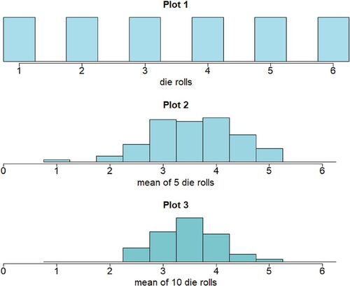
Fig. 1 Central limit theorem activity plots. Plot 1 shows the distribution of the outcomes of a die roll. Plot 2 displays the means of five die rolls observed during the activity and Plot 3 shows the observed means of 10 rolls.

The activity begins with a discussion of the Central Limit Theorem in which the instructor directs attention to the conditions and implications of the theorem. Namely, with repeated draws with replacement from a single population and a large enough number of draws (the conditions), the distribution of the sum or mean of draws will be approximately normal. The larger the number of draws, the closer to normal the resulting distribution is (the implications). Beginning statistics students often find it difficult to understand the CLT when it is initially stated. This simulation can be very effective in aiding them to connect statements such as ‘a single population’ and ‘large enough number of draws’ to a concrete context.

The first step in this activity is to connect the conditions of the central limit theorem to the simulation process students will engage in. As a class, we identify the distribution of the outcome of a die roll, plot this on the first of the horizontal axes (see Plot 1, Figure 1) and find the mean and variance of this distribution. Next, the instructor explains the data collection process and connects this to the conditions of the Central Limit Theorem.

The next step is for students to collect data from five die rolls. We instruct students to roll their die five times and to find the mean of the rolls. As they finish, students go to the second axis and place their sticky note in the bin that corresponds to their result, stacking multiple values in the same bin vertically. In this way, the class members work together to build a dot plot. Physically creating the dot plot engages students in the process and encourages them to think about the resulting distribution. Alternatively, students can report the mean of their 5 die rolls through an OSRS or by simply having students raise hands to indicate the appropriate bin as the instructor calls out bin endpoints.

The third step of this activity is to connect the results of the simulation to the implications of the Central Limit Theorem. The histogram of the mean of 5 die rolls has a fairly normal shape compared to the plot of the possibilities for a single die roll (see Plot 2, Figure 1). Students can also observe that the mean of the new distribution approximates the mean of the original distribution, and that the variance of the means is smaller than the original variance.

To illustrate that the distribution of the mean more closely resembles a normal distribution as the sample size increases, we do the experiment a second time, having each student roll the die and record the mean of 10 trials. Plotting the results of this experiment on the third horizontal axis, students will observe that the plot looks more normal, the mean is still approximately the same as in the previous two plots, and the variance of the newest distribution is smaller than those of the first two distributions (Plot 3, Figure 1).

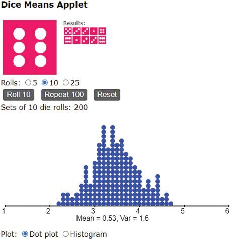
A variation on this activity has students flip coins and look at the distribution of the number of heads rather than rolling dice and looking at the distribution of the mean of the outcomes. Using coins has the advantages that many students can more easily access coins than dice and, more importantly, in many versions of the Central Limit Theorem, the results are stated explicitly in terms of the sum (see Freedman, Pisani, and Purves 2007). However, working with dice and the mean of rolls is advantageous because all three plots will have approximately the same mean, facilitating easy comparison between distributions. After attempting this activity recently in a somewhat smaller class, and being disappointed with the results, Schneiter (2022) created an applet that facilitates conducting the activity virtually (see Figure 2).

Fig. 2 An applet that facilitates simulation of the Central Limit Theorem die roll activity.

3.1.2 Confidence Level

Many textbooks show graphics displaying multiple confidence intervals to illustrate that the percentage that cover the true population parameter is approximately equal to the confidence level (see, e.g., Freedman, Pisani, and Purves. 2007; Moore, McCabe, and Craig 2009). When students physically explore this interpretation of confidence level, a large class size makes it easy to see the relationship between the confidence level and the percentage of confidence intervals constructed from random samples of the same size from the same population that capture the parameter.

This activity relies on an applet that facilitates drawing a random sample of words from The Gettysburg Address (Rossman and Chance 2022). Each student uses the applet to obtain a random sample of a specified size of words from The Gettysburg Address. The applet reports the mean and standard deviation of the lengths of the words in the sample and students use these to construct 95% confidence intervals for the mean length of all the words in The Gettysburg Address. Since the instructor knows the mean length of words in the address is 4.295 letters and can report this to students, each student is able to determine whether their computed confidence interval captured the parameter. The instructor can use an OSRS or simply ask students to raise hands to show how many intervals captured the true mean.

To emphasize this interpretation of the confidence level, the instructor asks students to recompute their confidence intervals using the same sample mean and standard deviation but changing the confidence level to 80% and again to 99%. After each iteration, the class finds the number of students whose confidence interval captured the parameter. With large class sizes, for an 80% confidence interval, about 80% of the class’s confidence intervals will capture the parameter and about 20% will not. For 99% confidence intervals, nearly the entire classes’ confidence intervals capture the parameter. This illustration of the meaning of the confidence level is not as evident in a small class. When we engage students in this activity in our classes, there are audible reactions of surprise from students as the confidence level and the percentage of students whose confidence interval captures the parameter nearly coincide.

3.2 Leveraging the Large Lecture for Inference

Much of statistical thinking is concerned with statistical inference: the practice of describing the attributes of a large population from a much smaller subset of the group. A large class has a clear advantage over a smaller one for engaging students in learning about inference through collecting real data to address inferential questions. If an instructor in a large class conducts an activity to answer a nontrivial question about the class as a population, it is evident to students that collecting data from the entire class would be time consuming and tedious. The utility of using sample data to draw conclusions about a population becomes immediately clear.

3.2.1 Hypothesis Testing

One activity that leverages a large class size to promote inferential thinking engages students in the process of hypothesis testing to determine whether the mean body temperature of class members is 98.6 °F. Though many people think of 98.6°as a typical human body temperature, some research has suggested that this might not be accurate (Mackowiak, Wasserman, and Levine 1992). Determining whether the mean body temperature of class members is consistent with this conventional wisdom naturally suggests the need for inference. The question requires measurement of the body temperature of students and thus cannot be easily answered in a poll or with an OSRS. Furthermore, it would be time consuming to measure the body temperature of every member of the class to ascertain the true mean. Thus, using a sample to draw conclusions about the large population is a reasonable and natural alternative.

Since the motivating question for this activity requires comparing the mean body temperature of students in our class to the usual claim of 98.6°, a hypothesis test is the expected method of analysis. When we engage in this activity, students have been introduced to this five-step process for hypothesis testing:

1. State the null and alternative hypotheses.

2. Collect data.

3. Calculate a test statistic.

4. Compute a p-value.

5. Draw conclusions.

We address each of these steps explicitly as we engage in the activity.

1. State the hypotheses. The parameter of interest for this experiment is µ, the mean body temperature of all students in our class. The nature of the question under consideration makes it simple for students to identify the null hypothesis, H₀: µ = 98.6 °F. This illustrates the idea of the null hypothesis as a statement of the status quo or what is expected. We then determine as a class what the alternative hypothesis should be, thus demonstrating that this is up to the discretion of the researcher(s). Because some studies have suggested that the mean typical human body temperature is lower than 98.6°, the students often choose to reflect that in that alternative hypothesis, H_A: µ <98.6°. This stage provides an excellent opportunity to reinforce with students the need to identify hypotheses before collecting data.

2. Collect data. The main challenge with collecting data for this experiment is identifying a random sample of class members. We have done this in various ways. At times, we’ve had students count off and used software to select random numbers that determine the participants. This requires no preparation and allows us to specify the sample size but is not the most efficient method. A better choice is to prepare tokens beforehand. The tokens should be of two types that are easily distinguishable visually but can’t be identified by touch. We have used beans; similarly shaped, wrapped candies; or marked pieces of paper with success. To use this method, we first decide what percentage, P, of the class we’d like to include in the sample. Next, we fill the bags with tokens such that the total number is approximately equal to the expected attendance, P% of the tokens are of one type (sample tokens) and the rest are the other. Students draw a token from the bag as they enter the classroom. Those who draw token 1 are invited to be part of the sample. Using this method to select the sample, the sample size depends on the number of students who attend and whether they choose to participate.

   When it is time to carry out the experiment, students who received “sample tokens” are invited to go to the front of the classroom. Because this experiment involves personal information, it is important to approach the data collection carefully, to explain the process to students before proceeding, and to give students the option of declining to participate. The instructor can use an infrared thermometer that is briefly held to the temple of each participant to take measurements without touch. As the temperature is measured, the instructor writes it down rather than reading the result to the class. The temperatures are read anonymously to the group once all sample participants have had their temperatures taken.

3. Calculate the test statistic. Once all students have access to the sample data, they can work in groups to compute summary statistics and find the value of the test statistic. Because these data are not collected in ideal circumstances, we have found that the sample mean is often much smaller than the null value of 98.6. This results in a test statistic with a large magnitude and provides a great opportunity for students to consider the information the test statistic contains and to anticipate what the final conclusions will be. We typically discuss this before moving on to talk about the p-value.

4. Compute the p-value. Again, students are encouraged to work in groups to compute the p-value and to discuss its interpretation. As mentioned previously, our test statistic is often large in magnitude, resulting in a very small p-value. We use these results to emphasize the interpretation of the p-value and whether it is possible for the p-value to be very small if the null hypothesis is true.

5. Draw conclusions. This step tends to be interesting for students since we are addressing a real and relevant question. The conclusion of the experiment tends to be that we reject the null hypothesis and conclude that the mean body temperature of our class is likely lower than 98.6°.

3.3 Discussion

In an activity, such as the body temperature activity described above, a large class is the population of interest. This drives home the point that, with a large population, the true value of the parameter can be out of reach. Students see, in a personal way, that sampling is an accessible alternative to a census. Recommendations vary about the maximum size of a sample in comparison to a population that will allow treating sample observations as independent but typical values are between 1% and 10%. In a class of over 100 students, 5% of the class gives a sample that is large enough to conduct the activity and demonstrate the principles and utility of inference. Moreover, the relatively large ratio of sample size to population size can motivate discussion about choosing an appropriate sample size and limitations of the inferential processes.

The classroom is not an ideal experimental setting, but this knowledge can be used to the instructor’s advantage to motivate discussions about sample size, experimental design, and messy data. For instance, when we have obtained a sample mean in the temperature experiment that is much lower than 98.6°, and after we talk about how “cool” our class is, the unexpected result leads to productive discussion about our experimental methods and generalization.

Instructors can also use technology to leverage a large class size to teach the ideas of hypothesis testing. Using OSRS polling, many simple questions can be answered quickly by the entire class even when it is a large one. Here too, a large class size can be advantageous. The instructor can pose a question to the class such as “Do you believe in ghosts?” a timely topic in the fall semester. Having obtained data from the entire class, the instructor knows the value of the population parameter. She can obtain a simple random sample of class members and ask those students to respond to the question a second time via the OSRS. Students compute an estimate of the parameter and the standard error and then compare these to the known value of the parameter and discuss these values in context.

3.4 Student Response

Students’ responses to these activities have been very positive. Many students have commented in course evaluations that they have enjoyed and learned from these activities. The activities have helped students to remain engaged and connected in what can be an isolating environment. The following comments from end-of-semester evaluations demonstrate this.

I loved the in–class experiments that we did! I was surprised that [the instructor] did them, since the class was so large. They were definitely a success in my book. It helped break up the lecture and helped me to understand the concepts much more when it was data we gathered as a class.

I liked the hands—on, in—class examples we did. Like [names specific experiments]. Those helped to cement ideas and concepts in my brain.

[The instructor] was good about using real data and actual examples to teach us concepts. And we frequently collected our own data, which was interesting and educational for us.

4 Conclusion

Statistics is a subject that many students approach with apprehension. This feeling may be augmented by the trend at many universities toward large class sizes since these make it harder for students to connect with their instructor and classmates. However, the role of “large” in statistics puts it in a unique position with respect to these big classes. Statistics instructors can leverage the large class size in a way that is peculiar to our discipline. We can capitalize on large class sizes to engage students in active learning and collecting data and can use technology to do this efficiently and effectively. Such lessons help students to see statistics in practice and to engage with their classmates despite the size of the class. Since students are involved in collecting and analyzing the data, the data come with their own relevance and interest. The increased engagement, personal relevance, and active learning can all lead to improved student attitudes toward statistics, less anxiety, and application of the GAISE recommendations in a large class setting. We have found that engaging with students in these activities promotes a greater appreciation of what Florence Nightingale called “the most important science in the world” (Cook 1913 as cited in Maindonald and Richardson 2004).

References

- Aliaga, M., Cobb, G., Cuff, C., Garfield, J., Gould, R., Lock, R., and Witmer, J. (2005), “Guidelines for Assessment and Instruction In Statistics Education: College Report,” American Statistical Association. Available at https://www.amstat.org/asa/education/Guidelines-for-Assessment-and-Instruction-in-Statistics-Education-Reports.aspx.
- Blair, R. M., Kirkman, E. E., and Maxwell, J. W. (2018), “Undergraduate Programs in the Mathematical Sciences in the United States: Fall 2015 CBMS survey,” National Science Foundation. Available at http://www.ams.org/profession/data/cbms-survey/cbms2015-Report.pdf.
- Carver, R., Everson, M., Gabrosek, J., Horton, N., Lock, R., Mocko, M., Rossman, A., Rowell, G., Velleman, P., Witmer, J., and Wood, B. (2016), “Guidelines for Assessment and Instruction in Statistics Education (GAISE) College Report Revised,” American Statistical Association. Available at https://www.amstat.org/education/guidelines-for-assessment-and-instruction-in-statistics-education-(gaise)-reports.
- Cline, K., and Zullo, H., eds. (2011), Teaching Mathematics with Classroom Voting: With and without Clickers, Washington, DC: Mathematical Association of America. DOI: 10.1017/CBO9781614443018.
- Cook, E. T. (1913), The Life of Florence Nightingale, London: Macmillan.
- Gelman, A., and Nolan, D. (2017), Teaching Statistics: A Bag of Tricks (2nd ed.), Oxford: Oxford University Press.
- Freedman, D., Pisani, R., and Purves, R. (2007), Statistics (4th ed.), New York: W.W. Norton.
- Hoang, H., Huang, M., Sulcer, B., and Yesilyurt, S. (2017), “Carnegie Math Pathways 2015–2016 Impact Report: A Five-Year Review,” Carnegie Foundation. http://www.carnegiefoundation.org/resources/publications/carnegie-math-pathways-2015-2016-impact-report-a-five-year-review/.
- Kvam, P. H. (2000), “The Effect of Active Learning Methods on Student Retention in Engineering Statistics,” The American Statistician, 54, 136–140.
- Lane, D. (2018). “Sampling Distributions,” Available at https://onlinestatbook.com/stat_sim/sampling_dist/index.html.
- Mackowiak, P. A., Wasserman, S. S., and Levine, M. M. (1992), “A Critical Appraisal of 98.6 F: The Upper Limit of the Normal Body Temperature, and Other Legacies of Carl Reinhold August Wunderlich,” Journal of the American Medical Association, 268, 1578–1580. DOI: 10.1001/jama.1992.03490120092034.
- Maindonald, J., and Richardson, A. M. (2004), “This Passionate Study: A Dialogue with Florence Nightingale,” Journal of Statistics Education, 12. DOI: 10.1080/10691898.2004.11910718.
- Moore, D., McCabe, G., and Craig, B. (2009), Introduction to the Practice of Statistics, New York: W.H. Freeman.
- Muir, S., Tirlea, L., Elphinstone, B., and Huynh, M. (2020), “Promoting Classroom Engagement Through the Use of an Online Student Response System: A Mixed Methods Analysis,” Journal of Statistics Education, 28, 25–31. https://doi.org/10.1080/10691898.2020.1730733.
- Rossman, A., and Chance, B. (2022, February 12). “One Variable with Sampling,” Available at https://www.rossmanchance.com/applets/2021/sampling/OneSample.html?population=gettysburg.
- Schneiter, K. (2018), “The Law of Averages,” Utah State University. Available at https://www.usu.edu/math/schneit/Statlets/LawOfAverages/.
- Schneiter, K. (2022), “Dice Means,” Utah State University. Available at https://www.usu.edu/math/schneit/Statlets/DiceMeans/.
- Singer, J. D., and Willett, J. B. (1990), “Improving the Teaching of Applied Statistics: Putting the Data Back into Data Analysis,” The American Statistician, 44, 223–230.