Teaching Monte Carlo Simulation with Python

Abstract

It has become increasingly important for future business professionals to understand statistical computing methods as data science has gained widespread use in contemporary organizational decision processes in recent years. Used by scores of academics and practitioners in a variety of fields, Monte Carlo simulation is one of the most broadly applicable statistical computing methods. This article describes efforts to teach Monte Carlo simulation using Python. A series of simulation assignments are completed first in Google Sheets, as described in a previous article. Then, the same simulation assignments are completed in Python, as detailed in this article. This pedagogical strategy appears to support student learning for those who are unfamiliar with statistical computing but familiar with the use of spreadsheets. Supplementary materials for this article are available online.

KEYWORDS:

• Statistical Computing
• Python programming
• Spreadsheets

1 Introduction

Two semesters of applied statistics are required for undergraduates pursuing a business degree at the corresponding author’s institution, which is an Association to Advance Collegiate Schools of Business (AACSB) accredited School of Business within a regional state university. Previously, these business statistics courses would have included applied data analysis using commercially produced software programs in the curriculum. However, the field of applied statistics has moved toward free and open-source statistical computing platforms, making commercial programs less pertinent. In an effort to make statistics as relevant as possible to the future business careers our students will pursue, I, the corresponding author, began teaching a statistical computing module using Python as part of the second-semester statistics course. Initially, I incorporated statistical computing with Python into the curriculum with two free learning platforms, Datacamp.com and Repl.it, and evaluated their effectiveness in teaching programming skills to undergraduate students with limited, if any, programming backgrounds (Holman 2018). A deeper analysis of the decision to use DataCamp’s resources can be found in Holman (2018), in which I conclude that “I still recommend DataCamp as a good source of material for training data scientists but I do not suggest relying on the interactive exercises as a reliable indication or measurement of student comprehension” (109). In the next iteration of the course, I introduced Monte Carlo simulation with spreadsheets as a pedagogical tool to better support student learning of a new programming language (Holman 2019). In this article, the coauthor and I describe the sequence of Python programming exercises used to teach Monte Carlo simulation and analyze their effectiveness.

2 Literature Review

In recent years, demand has increased dramatically for programming and data analysis skills (Manyika et al. 2011; Davenport and Patil 2012). As a result, AACSB-accredited Business Schools have begun offering targeted coursework and programs in business analytics and data science (Brunner and Kim 2016; Zhao and Zhao 2016). An awareness of the importance of quantitative literacy for a variety of disciplines, particularly in probability and statistics, has risen in the past two decades as well (Hallett 2003). Accordingly, instructional strategies for data science courses have received recent attention in both statistical and pedagogical literature. A consistent theme is the need to give students opportunities to practice and apply programming techniques and languages like Python to realistic problems, both in and out of the classroom (Rufinus and Kortsarts 2006; Dichev et al. 2016; Woodard and Lee 2021). Similarly, statisticians have started to advocate for the inclusion of computing concepts in undergraduate statistics curricula (Nolan and Temple Lang 2010; Donoho 2015). This shift began in the early 2010s with a call from the American Statistician Association (ASA) to improve undergraduate curricula, to more effectively prepare both statistics students and interdisciplinary students for their future careers (Horton and Hardin 2015).

In their revised Guidelines for Assessment and Instruction in Statistics Education (GAISE) College report released in 2016, the ASA added two additional emphases to the recommendation “teach students statistical thinking,” pushing for that to be in the context of investigative processes of problem-solving and decision-making and to include multivariable thinking (GAISE College Group 2016, 6). Additionally, the GAISE recommendations include “gain[ing] experience with how statistical models are used” and “interpret[ing] and draw[ing] conclusions from standard output from statistical software packages” (GAISE College Group 2016, 8). Simulation and statistical modeling meet these criteria and as a result, entire statistics courses have been framed around simulation exercises (Nolan and Speed 1999; Nolan and Temple Lang 2003; Horton, Brown, and Qian 2004; Foster and Stine 2006; McLoughlin 2008; Horton 2013). Many of these simulation exercises operate along the same lines of thinking as Batanero, Tauber, and Sánchez in arguing that students develop an understanding of mathematical and statistical concepts by solving problems related to that concept (Batanero, Tauber, and Sánchez 2004). Such simulations can also encourage them to make real-life connections through examining risk in the world of financial investment (Foster and Stine 2006) and allow them to work with real data, defined by Gould (2010) as “associated with real people and places and collected to solve and answer a specific and pressing questions” (5). Both of these examples demonstrate how integrating simulation exercises into statistics courses allows further opportunities to meet the guidelines and recommendations set by the American Statistical Association by making the coursework more relevant and accessible to students. Additionally, similar arguments in favor of providing students opportunities for contextualized experience with statistical simulation in order to better prepare them for the workforce have been made in fields outside of business analytics, including engineering and chemistry (Barba, Wickenheiser, and Watkins 2017; McCluskey et al. 2019). These additional cross-discipline studies demonstrate an overall shift in the world of statistical computing to emphasize the real-world application of such skills and better prepare students for the reality of the workforce.

In this article, we will build on these pedagogical strategies by introducing a scaffolded Monte Carlo simulation as an exercise to learn Python. Research shows that this mathematical tool, which is used to estimate outcomes in cases of risk or uncertainty, has incredibly broad applications in statistical computing. The Monte Carlo method was introduced by Metropolis and Ulam (1949) and has been applied extensively in many fields including biology (Manly 1997), physics (Strawderman 2001), engineering (Arie 2000), and finance (Glasserman 2004). It has also been applied through Python programming to research in a variety of disciplines, ranging from MRI data to earth science (Karssenberg, de Jong, and van der Kwast 2007; Kerkelä et al. 2020). Though Monte Carlo simulation is not usually included in a business statistics curriculum, it has proved to be useful pedagogy for teaching production and operations management (Usher 2008; Hayes 2008), economics (Becker and Greene 2001; Craft 2003), finance (Carver 2013) and more traditional business statistics topics including Sampling Distributions and Hypothesis Testing (Weltman 2015, 2017). Finally, recent research argues that modeling and simulation are constructive to students’ statistical learning to provide opportunities to diagnose unexpected outcomes (Peng et al. 2021), a criterion Monte Carlo simulation provides because it produces a full range of outcomes, including those that are less likely or unexpected. This article builds on these pedagogical applications to business curriculum concepts generally and draws from Carver (2013) to provide a set of teaching exercises specifically designed for analysis of financial data while also engaging students in the application of the programming language Python.

When it comes to the software package used for simulation modeling, some statisticians advocate the use of the R language (R Development Core Team 2006) in statistics curricula to teach students programming language skills (Nolan and Temple Lang 2010). As described by Horton, Brown, and Qian (2004), R can be used both for statistical analysis by professionals and as a classroom tool for exploration. Indeed, students pursuing a degree in statistics or data science would be well served to learn both R and Python. For undergraduate business students taking required courses in statistical methods, there is not sufficient time built into the curriculum to properly introduce both the R and Python environments. As a result, and due to its broad applicability and growing popularity, Python seems to be the more practical option.

In recent years Python has received increasing support for teaching data science and programming skills (Brunner and Kim 2016). According to the Python Software Foundation (2021), “Python is an interpreted, interactive, object-oriented programming language which combines remarkable power with very clear syntax.” Many researchers and instructors also emphasize Python as a preferred language for instruction because it is so marketable and its simplicity allows students to focus on the programming and problem-solving skills rather than the complex syntax of other programming languages (Rufinus and Kortsarts 2006; Brau, Brau, and Keith 2020). While R is restricted to statistical computing applications, Python is a general-purpose programming language like Java or C + + and can be used for a wide variety of purposes, which helps prepare business students in particular for the workforce (Perkel 2015). Brunner and Kim (2016) also argued that “Python (especially when using the Pandas library) is capable of performing most, if not all, of the data analysis operations that a data scientist might complete by using R” (1948). More recently, the Institute of Electrical and Electronics Engineers (IEEE) ranked Python as the number one overall programming language (Cass 2020). In 2018, they observed that R’s slight decline in their rankings likely contributed to Python’s continued success, stating “the existence of high-quality Python libraries for both statistics and machine learning may be making flexible Python a more attractive jumping-off point than the more specialized R” (Cass 2018). In 2020s report, Cass also argued that Python’s sustained popularity can be attributed to its frequent use as a teaching language, further supporting its presence in undergraduate curricula.

Researchers have found Python to be an increasingly desirable skill for employers in both data science and business analytics and concluded that its tremendous community support has increased its utility in the workforce and its desirability for teaching at the collegiate level (Stanton and Stanton 2020). Usage statistics continue to underscore the advantages of Python. According to Stack Overflow (2018), a popular online forum for programmers, growth in the use of Python versus other popular programming languages is unsurpassed since 2012. In its most recent survey, Stack Overflow (2021) reports usage of Python at 48.24% versus Java at 33.35%, C + + at 24.31%.

Python is easy to learn and even described as “a joy to teach” because of its simplicity and practicality (McCane 2009, 10). This sentiment comes primarily from an introductory programming standpoint but it still has some relevance in business analytics. More generally, quantitative evaluation of teaching introductory programming with Python versus Java indicated that Python is preferred for teaching basic, procedural aspects of programming and Java is more appropriate for teaching object-oriented programming (Jayal et al. 2011). Furthermore, significant literature emphasizes Python’s accessibility as a programming language for undergraduate students with little to no background knowledge in programming, which best describes the background of the majority of students in this course.

3 Course Description

The University catalog describes Advanced Business Statistics as follows: “Development of advanced statistical techniques to support business decision-making. Topics include advanced multiple regression analysis, analysis of variance, and nonparametric techniques.” The course is the second in a required two-course sequence within the School of Business, following the prerequisite first-semester course, titled “Inferential Statistics and Problem Solving.”

In Spring 2019 the course was taught in a computer lab classroom with 45 Dell Personal Computers (PCs) connected to the internet, running Microsoft Windows, and equipped with the Microsoft Office suite and other popular software applications for business productivity. The course met for 80 minutes twice per week for 15 weeks in a traditional format. Although web materials and web applications were used frequently, the course was not an officially designated “hybrid” or “online” course, and students were expected to attend class in person. There were two sections of the course with the first section beginning at 11:15 a.m. and the second beginning at 1:00 p.m. each Monday and Wednesday of the semester. A total of 79 students were enrolled in both sections combined. Students were encouraged to work together on assignments but required to submit their own work. Three exams were used to assess student proficiency. A course syllabus and individual lesson plans with detailed assignments, including Python programming assignments, are available by contacting the author.

4 Simulation Lessons

Though a detailed accounting of every aspect of the content delivered in the Advanced Statistics course during the Spring 2019 semester is beyond the scope of this article this section describes the ways in which the Python simulation module is presented to students. In Holman (2019), the corresponding author described the instructions for first implementing these three simulations in Google Sheets, before moving on to repeat the same simulations using Python.

While few business students had experience with computer programming coming into the course, nearly every student had experience with spreadsheets, primarily using Microsoft Excel due to its near-ubiquitous presence in the business world. Despite this, this coursework scaffolds their experience of learning Python programming with Google Sheets instead. Google Sheets is nearly identical to Excel in function but is a “pure” web application, which eliminates concerns about compatibility given the vast variety of mobile and desktop student computing devices.

As they are completing each of the simulation lessons in Google Sheets, students also begin an introductory Python programming module using a combination of courseware from DataCamp and instructor-led in-class programming activities utilizing the Repl.it on-line development environment. DataCamp provides video and interactive programming lessons at no cost for classroom use at datacamp.com (DataCamp 2019). Students began with “Intro to Python for Data Science” where they were introduced to Python Basics, Lists, Functions, Methods and Packages, including NumPy, an extension module created to facilitate numerical computation (Oliphant 2006; Harris et al. 2020). While DataCamp serves to communicate and teach the essentials of Python, Repl.it is a browser-based development environment for Python and other programming languages that provides a space for students to practice what they are learning by writing code (Repl.it 2021). It is useful both because it is a platform-independent online environment and because it is easy to share and troubleshoot programs by simply copying and pasting a web link.

In summary, students learn the simulations in Google Sheets while they are also learning the basics of writing Python through the lessons in Datacamp. Then, they apply that knowledge of both Python basics and Monte Carlo simulation exercises by crafting the simulations themselves in Python using Repl.it. Below, we briefly describe the exercise students completed for each simulation, along with a model of the work required to run the simulation in Python using Repl.it, and the pedagogical implications of each. A line-by-line description of the simulation is beyond the scope of this article, but can be found in the supplementary materials.

4.1 Simulation 1: Coin Toss

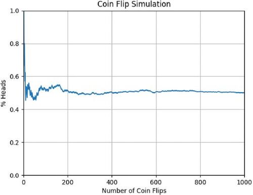
Initially, students are introduced to the coin toss, one of the simplest possible random processes. In this exercise, students are asked to consider how the accuracy of forecasting the outcome of the coin toss changes with greater repetition. The intended learning outcome is that students are able to describe how accurately predicting a single coin flip is very difficult but, as the number of iterations increases, predicting the proportion of heads or tails becomes increasingly accurate. This sounds elementary, but hopefully, students recognize that the same simulation approach can be applied to other, more complex, processes with similar opportunities in terms of prediction accuracy. Using a simple “for loop,” a Python program iterates through multiple coin tosses. There are no inputs or parameters. Rather, this simple simulation illustrates that as the number of coin tosses increases, the mean probability of coin tosses that result in “heads” converges toward 0.5. See Figure 1 or interact with the program directly by browsing to https://replit.com/@statsprof/Sim1CoinToss. Note that although Python loops are known to be relatively inefficient, no performance lags were observed during classroom simulation tests with up to 10,000 iterations.

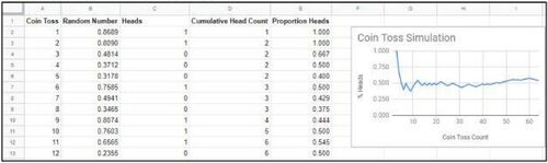
Fig. 1 Coin toss simulation in Google Sheets, used to scaffold student learning in Python (Holman 2019).

In the Python program above, shown in the Repl.it development environment, there are 20 lines of Python code in the file, main.py. Line 2 of the program imports the “random” module used to generate random numbers. There are four total variables: “sims” for number of simulated coin tosses, “simcount” and “heads” for integer counting variables, and “pcth” to calculate the “percent heads” result at each step in the simulation. As mentioned before, the substance of the program begins with a “for loop” which tells Python to loop through the simulation ten thousand times for the student assignment, but can be modified to any integer. Once the coin toss has been simulated, a conditional statement checks to see if the random number is greater than zero, which is the “heads” outcome, and the “heads” variable increases accordingly. As the heads variable changes, so does the “pcth” variable so that the percent heads is constantly being updated as the simulation runs. The idea is to show that early on in the iterations, the percentage of heads is fairly volatile, but it eventually begins to converge toward 0.5. The higher the number of iterations, the more complete the convergence, which is why students are asked to repeat the simulation with higher numbers of iterations each time. With only 100 iterations, the range of possibilities is wider, anywhere from 0.4 to 0.6 is likely, but at 1,000 or 10,000 iterations, the range narrows and is highly likely to be within a few one-hundredths from 0.5 by the end of the simulation.

The program in Figure 2 contains everything necessary for the simulation. The remaining lines of code, shown in Figure 3, generate a lineplot for visualization showing how the percentage of coin tosses resulting in “heads” converges to 0.5. This component of the exercise is both an appropriate skill for students to practice in Python and serves to reiterate the objective to students, ensuring that their takeaway from this simulation is that greater repetition leads to convergence and predictability. Two very commonly used Python modules are imported, NumPy and matplotlib, to facilitate the creation of a line plot. The list variable, “pcth” or “percent heads,” is converted into a NumPy array, which is passed to the “plot” function creating a line plot. Note that matplotlib can typically plot a list variable but in Repl.it the line plot was not rendering properly until the NumPy array was utilized. On lines 30–36, graph attributes are defined and the “show” command tells the program to display the resulting graphic. See Figure 3 as well as the supplementary materials for coding details and see Figure 4 for the resulting graphic output.

Fig. 2 Coin toss simulation in Python on Repl.it: https://replit.com/ @statsprof/Sim1CoinToss.

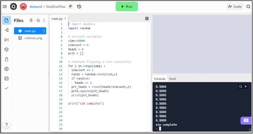
Fig. 3 Coin toss simulation graphic output on Repl.it: https://replit.com/ @statsprof/Sim1CoinToss.

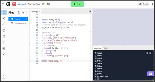
Fig. 4 Graphic displaying repeated trial results for coin flip simulation.

4.2 Simulation 2: Dice Game

In the second simulation, students are introduced to another relatively simple discrete probability distribution. It involves repeated randomization of rolling a pair of dice, evaluating the outcome, and then calculating the resulting change to a hypothetical player’s cash balance. Students are specifically asked to simulate a simple game called “Lucky Seven” in which all rolls other than a seven result in a losing bet while rolling a seven is rewarded with a relatively large payoff. The objective of the exercise is to run the simulation under various payoff scenarios, in which the payoff multiplier for a winning roll could be four, five, six, or seven times the bet amount. Then, they use the simulation to decide which payoff amount will both draw potential game players and earn profit for the casino.

A new element introduced in this simulation is the financial outcome component. An initial balance is established and the balance is updated after each roll of the dice. This enables students to analyze various payoff levels and how winnings are then distributed between the “player” and the “house” after many iterations. The program is displayed in Figure 5, in the supplemental materials, and on repl.it at https://replit.com/@statsprof/Sim2DiceGame.

Fig. 5 Dice game simulation on Repl.it: https://replit.com/@statsprof/Sim2DiceGame.

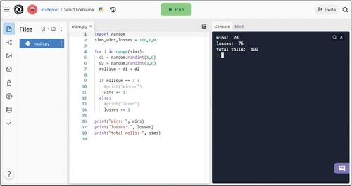
This program starts the same way as the coin flip simulation—with a Python module for random variable generator, using another “for loop” at the core of the simulation. However, instead of randomly choosing between integers zero and one, the range of the random variable generator increases from between one and six to mimic the roll of a single die. Likewise, it must be inserted twice in the code to simulate the roll of two dice. If you generate a random number between two and twelve, to simulate the possible range of sums of those two dice, the outcome will be a uniform distribution. It will reflect an equal likelihood of rolling a twelve or a two as rolling a seven or a nine, even though in reality a roll of double ones or double sixes is far less likely than rolling a six, seven, or eight. Therefore, the same line is inserted twice before summing the two numbers to simulate the distribution of results from rolling two dice individually. This is the simplest of games involving dice: if you roll a 7 you win, if you roll any other sum you lose. Therefore, the sum has to be tested to determine if the roll is a win or a loss, increasing the respective variable by one.

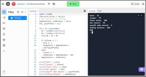
To extend the Dice Simulation to include a financial component, “begin balance” and “end balance” are added, along with the “bet” amount and the “pay off odds” variables. If the result is a win, the end balance will be equal to the beginning balance plus the bet amount times the payoff odds. This is expressed under “wins” in line 14 as “endbalance = beginbalance + (bet*payoffodds).” If it is a loss, the end balance will be equal to the beginning balance minus the bet amount. That will be expressed in line 17 (under “losses” in line 16) as “endbalance = beginbalance—bet.” At the end of the “for loop,” the beginning balance needs to be reset to reflect the end balance. That way, it will accurately reflect the impact of wins and losses for each subsequent roll of the two dice. See Figure 6, the supplemental materials, or browse to https://replit.com/@statsprof/Sim2DiceGame-PlusBetting for details.

Fig. 6 Dice game simulation with betting: https://replit.com/@statsprof/Sim2DiceGame-PlusBetting.

When a pair of dice are rolled, there are 36 possible outcomes. and 6 of those outcomes result in rolling a 7. Therefore, the probability of rolling a 7 is 6/36, which is 1/6 or approximately 16.67%. Once again, though there will be some initial variability, as the number of simulations increases, the probability of winning the game and rolling a 7 should get closer and closer to 16.67% overall. Possible extensions to this assignment are as numerous as the number of dice games that can be simulated. Prompting students to implement alternative rules is an excellent way to test and enhance their comprehension.

After presenting the Lucky 7 game simulation, students are asked to implement a simplified version of craps called “Pass” where the player wins with a roll of 7 or 11, loses with a roll of 2, 3, or 12 and ties with rolls of 4, 5, 6, 8, 9, or 10. As a more challenging assignment, students are asked to implement a game called “Chuck-a-luck” which involves tossing three dice and winning a large payout for rolling a “triple,” that is, three of a kind.

4.3 Simulation 3: Stock Market Returns

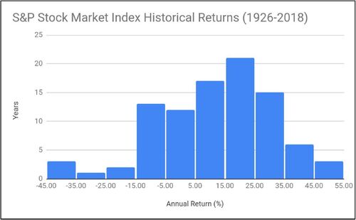
The stock market simulation is the most complex, but by this point in the course, students are familiar with most of the elements utilized in the model. First, we look at the distribution of historical stock market returns. Using the S&P 500 and going back to 1926 we generate a frequency distribution of historical total returns and observe that the distribution is skewed but approximately normal with a mean of 11.88% and a standard deviation of 19.76%. See Figure 7 for details. Students are cautioned that the assumption of normality may skew results and is made to facilitate a simpler simulation. Students are also instructed to identify the distribution of data they may want to simulate in the future, which may not be normally distributed.

Fig. 7 Distribution of S&P 500 Stock Market Index annual returns (%) from 1926 to 2018.

Using the information provided above and the simulation described below as a starting point, students are then asked to implement the necessary program elements to track a hypothetical retirement portfolio over a 40-year time frame. This exercise is very intimidating and difficult for novice programmers but using the spreadsheet model to scaffold instruction as described in Holman (2019) as a guide along with the code for tracking bets in the Dice Simulation (see Simulation 2 and Figure 6), students typically complete the assignment successfully.

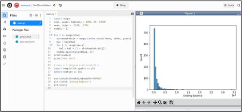
In this simulation, similar to the way the random module was imported, the “NumPy” module is imported (numpy.org). Then, the variables are established as number of simulations, years, and beginning balance. The mean and standard deviation of the stock market return data, which are taken from Figure 6, are integrated in line 3. Next, another loop is established to simulate the stock market assuming a normal distribution and using the “normal” function passing the mean, standard deviation, and the number of years as parameters. The loop goes through the 40 years starting with the beginning balance increased by the return from stock market simulation in the previous loop’s iterations. The simulation concludes in lines 12 to 14 with the ending balance that has the list of returns, which prints before the simulation ends. See details in Figure 8, the supplemental materials, or browse to the repl.it program at https://replit.com/@statsprof/Sim3StockMarket.

Fig. 8 Stock market simulation: https://replit.com/@statsprof/Sim3StockMarket.

Students are given the program in Figure 8 then asked to calculate several summary statistics. Students are also asked to use the simulation to estimate the likelihood of reaching a particular target balance within a specified number of years. After students have gained familiarity with the stock market simulation they are asked to add a fixed income (bonds) component, or other asset classes (e.g., gold, cash, international stocks), to the simulation. In addition, students must implement the ability to designate a percent stocks and percent bonds (or other asset class), for example, 80/20 or 60/40, as a portion of the total investment portfolio with annual rebalancing.

5 Student Evaluations

Although a formal experimental design with control groups is beyond the scope of this article, voluntary student evaluations at the author’s institution can be used as anecdotal evidence to reflect the impact of this pedagogical strategy on students. These evaluations are submitted near the end of the course, and because they are voluntary, respondents are self-selected, not randomly determined. Students are presented with 18 different categories for which they select ratings on a scale with 5 options (i.e., Strongly Agree, Agree, Neutral, Disagree, Strongly Disagree) and are subsequently prompted to provide text responses reflecting on instructor approachability, what works well and what to improve.

In the spring semester of 2018, the corresponding author introduced Python through DataCamp lessons and Monte Carlo simulations but without first introducing simulation exercises in spreadsheets. That semester, out of 79 possible respondents in the class, 35 students completed an evaluation yielding a response rate of 44%. Of the 35 evaluations completed, 28 students provided text comments in response to the “What works well?” prompt with the word “Python” appearing 6 times. And, 29 students provided text comments to address “What to improve?” with the word “Python” appearing 11 times. Comments submitted are listed under “Student Evaluation Data” in the supplementary materials.

Clearly, from the comments submitted, not all students included only positives of the course in their response to the first question, nor did they include only suggestions for improvements in their answer to the second question. Because many students included both positives and negatives together in their answers, the two collections of responses are best analyzed together. Many of those positive and negative comments applied to the grading and pacing of the course, which while useful, are not pertinent to this article. However, multiple mentions of in-class work on solving problems were mentioned as positive, which is a hallmark component of teaching simulations. Additionally, more than five students praised the real-life application of the work they learned and completed in this course, several of them specifically linking it to Python’s many applications to their future careers, which was a driving force for including it in the coursework in the first place. Several students also argued that more time should have been dedicated to Python. This is productive feedback that demonstrates the general advantages of learning Python, while also informing potential structural changes to future iterations of the course.

The evidence leads me to conclude that Python was not consistently popular or unpopular with all students. While some comments were critical of the use of Python programming as part of the course, others specifically mentioned Python as a positive element. That said, it’s difficult to know whether the same students might have taken issue with being assigned running and interpreting multiple regression models in SPSS or similar, which would have required extensive time by nature.

In the spring semester of 2019, the corresponding author continued to teach Python with DataCamp lessons and Monte Carlo simulations. However, exercises introducing Monte Carlo simulations in Google Sheets were added to the first half of the course in order to scaffold student learning as they approached Python with the same simulations. This semester, the student evaluations yielded a response rate of 57%, with 43 students answering out of 76 possible respondents in the course. Of the 43 evaluations completed, 36 students provided additional text comments in response to the “What works well?” prompt with the word “Python” appearing 7 times. Additionally, 32 students provided text comments to address “What to improve?” with the word “Python” appearing 13 times. Comments submitted are listed in the supplementary materials.

Though many comments again make suggestions more focused on grading and assignments, with regard to Python, this evidence once again shows that students are divided in their view. While some comments specifically mention Python in a positive light, other comments mentioning Python are critical of its role in the course. Once again, five students praised the in-class demonstration, hands-on problems, and the practical applications of the assigned problems. Five students specifically praised the inclusion of outside technology like DataCamp, and several students also described the real-life utility of Python across disciplines. Several negatives were presented by students as well, though many of them appeared to be related to the challenging nature of the course, and it is possible these students exhibit a negative response to most challenging stimuli. On the other hand, there are legitimate concerns expressed by students regarding how much time is devoted to learning Python, how content is delivered in class and out of class, and how much breadth and depth are appropriate. These comments can be used to inform improvement in terms of both content and instructor delivery.

Table 1 compares ratings between the two Advanced Statistics course sessions in Spring 2018 and Spring 2019. Again, instead of looking at the numerical rating averages, I have simply provided the proportion of students indicating they “Strongly Agree,” the highest (best) rating possible, with each question about the course.

Table 1 The proportion of students indicating that they “Strongly Agree” with each question about the course is shown here for the 2018 Spring and 2019 Spring Advanced Statistics Course.

	2018	2019
Question text	Advanced statistics	Advanced statistics	Difference
Pace of course (is appropriate)	0.54	0.72	+ 0.18
Grading system is fair	0.71	0.86	+ 0.15
Prompt grading of work	0.71	0.84	+ 0.13
Instructor made use of class time	0.74	0.91	+ 0.17
Made difficult material understandable	0.60	0.70	+ 0.10
Communicates ideas clearly	0.63	0.81	+ 0.18
Responded to student questions	0.74	0.81	+ 0.07
Available outside of class	0.69	0.84	+ 0.15
Set and maintained high standards	0.71	0.86	+ 0.15
Encouraged critical thinking and analysis	0.74	0.91	+ 0.17
Instructor facilitated class participation	0.57	0.84	+ 0.27
Treated students with respect	0.83	0.88	+ 0.05
Communicated enthusiasm for the course	0.77	0.84	+ 0.07
Teaching strategies enhanced learning	0.63	0.72	+ 0.09
Text was effective	0.26	0.65	+ 0.39
Instructor was a successful teacher	0.66	0.91	+ 0.25
Learned from the course	0.66	0.79	+ 0.13
Average	0.66	0.82	+ 0.16

The noticeable increase in overall ratings across all categories for the course between 2018 and 2019 may demonstrate the effectiveness of the scaffolding approach to teaching Python, created by introducing Monte Carlo simulations in Google Sheets first and in Python second. In fact, one student’s evaluation comment specifically described this approach as a positive aspect of the course that supported their learning, responding “He went about teaching google sheets first to get us used to the soft-coding on that before moving along to Python. Great approach” to the question “What works well?” While these rating differences could be attributed to differences in the student cohorts or the comfort of the instructor with the materials, overall, the feedback and increased ratings support the hypothesis of this article that scaffolding the simulation lessons with spreadsheets before introducing Python programming makes learning programming more accessible to students.

The stated aim of the course is to teach advanced statistical methods. Some students believe this implies that the content should be akin to a “math class” rather than a “programming class” but we disagree. The most salient changes and advances in statistical methods over the past 30 to 40 years, in the business world and elsewhere, involve the application of computational methods to large datasets. These advances have both opened up opportunities to explore problems that were previously intractable and transformed the workplace. In the 20th century, no one thought of themselves as a data scientist, but in 2012 the role of data scientist was declared the “Sexiest Job of the 21st Century” in the Harvard Business Review (Davenport and Patil 2012). Some students have complained because learning computational methods is a more challenging task than learning how to operate a statistical software program like SPSS. These are students whose primary motivation is to minimize effort toward obtaining a degree. More ambitious students who are looking ahead at these trends in employment prefer to be exposed to the latest approaches and technologies. These are likely the same students providing evaluation feedback, available in the supplementary materials, with comments such as “the material I learned will be applied in the future” and “Datacamp gears things back to the real world.” If the curriculum was limited to a “pencil and paper” math class instructional modality, these forward-thinking students would rightfully be able to complain that the professor and the academy were not keeping up with the “real world” of private industry where they will almost certainly spend their career. Therefore, we believe including Python in the curriculum meets the stated aim of teaching advanced statistical methods for these students.

6 Conclusion

In 2020, Brau, Brau, and Keith described an Information Systems Course with programming-oriented learning objectives. Similar to this article, the course targeted students with no programming language experience and strove to provide them with contextualized, workforce-applicable examples of Python’s utility in future careers in the hands-on simulation portion of the coursework. Their student evaluation results indicated that the course explained concepts effectively, and comments reflected that the ways in which these advanced programming skills were taught helped students understand their application. This case study appears to reiterate the findings of this article that such hands-on, simulation-based programming courses are useful to students in preparing them for future careers.

In 2017, through a grant from the National Science Foundation, Dr. Lorena A. Barba and her fellow Mechanical and Aerospace Engineering department faculty at George Washington University designed a two-year program of Python computing modules to accompany their undergraduate engineering coursework (Barba 2020). As we argued in this article, Barba also emphasized the value of Python programming in preparing students for the workforce across many disciplines, including engineering. For this reason, the department created modules that incorporated simulation activities and computational skills through open-source resources like the Jupyter Notebook. In student evaluation data, the majority of survey respondents said they frequently used the skills they learned in the Python modules in their other coursework. It appears that the idea of simulation-based problem-solving as a way for students to experience computing in applied contexts supports student learning and workforce preparation across disciplines, meaning that simulations created for one course or department could possibly be beneficial to another as well.

Finally, scaffolding learning is a pedagogical tool the corresponding author, as the instructor, felt was critical to the student success in this course. The concept of scaffolding itself is widely attributed to Vygotsky (1978) and his research around the zone of proximal development. Maybin, Mercer, and Stierer (1992) built on this work to define scaffolding as “the process whereby one person in the role of ‘teacher’ mediates the progress of another person, the ‘learner’, by reducing the scope for failure in the task the learner is attempting” (23). Its applications to a variety of disciplines and pedagogical practices has been widely explored in the past fifty years, and the teaching of mathematics and statistics are no exception. Postsecondary instructors have argued that appropriate scaffolding materials are differentiated to groups of students in order to bridge their thinking from a familiar to an unfamiliar concept (Taber 2018) and should help students construct their own conceptual knowledge of a problem or idea by engaging in guided research and hands-on practice (Ruder, Stanford, and Gandhi 2018; Khusna 2021).

Overcoming the trepidation many students feel toward computer programming is a key challenge in teaching statistical computing. For most students, their experience in my Advanced Statistics course is their very first introduction to computer programming. However, nearly all business students have some familiarity with spreadsheets coming into the course. According to student data collected through end-of-course evaluations (Holman 2019), there was a wide range of responses to including Python programming in the curriculum, with some students believing a statistics course should include no programming elements while others wanted to spend more time on computational methods. However, the data did indicate that student familiarity with a spreadsheet environment made using Google Sheets as an introductory computing platform helpful in alleviating student anxiety around beginning Python programming. Because Monte Carlo simulation can be conducted in Google Sheets as well as in Python, it supports my efforts to scaffold student learning by allowing students to become accustomed to new simulations in a familiar spreadsheet environment, like Google Sheets, before transitioning to a new and more intimidating computational environment, like Python. With this in mind, a positive next step for the course is to continue experimenting with pedagogical approaches to introduce students to these important computational and statistical methods while working to mitigate their anxiety.

Scaffolding with spreadsheets to teach computational skills in Python offers a promising path toward filling a critical gap in workforce training and economic development found in, for example, the shortage of computational skills in the labor market. To continue assessing the spreadsheet-to-Python scaffolding approach described here, there are plans to next build comparable learning modules for teaching other advanced statistics topics such as multiple regression analysis and modeling in this and similar courses.

Supplementary Materials

Included in the supplementary materials is a line-by-line explanation of the Python code that students should input into the Repl.it environment to complete each simulation. Additionally, the full Student Evaluation Data is included in the form of course comments from the Spring 2018 and Spring 2019 semesters as evidence supporting the inclusion of Python in the course.

References

- Arie, D. (2000), Monte Carlo Applications in Systems Engineering, New York: Wiley.
- Barba, L. (2020), “Engineers Code: Reusable Open Learning Modules for Engineering Computations,” Computing in Science & Engineering, 22, 26–35.
- Barba, L., Wickenheiser, A., and Watkins, R. (2017), “CyberTraining: DSE—The Code Maker: Computational Thinking for Engineers with Interactive, Contextual Learning,” National Science Foundation CyberTraining Proposal, Accessed April 7, 2022. Available at https://figshare.com/articles/online_resource/CyberTraining_DSE_The_Code_Maker_Computational_Thinking_for_Engineers_with_Interactive_Contextual_Learning/5662051/1.
- Batanero, C., Tauber, L. M., and Sánchez, V. (2004), “Students’ Reasoning About the Normal Distribution.” in The Challenge of Developing Statistical Literacy, Reasoning and Thinking, eds. D. Ben-Zvi and J. Garfield, 257–276. Netherlands: Springer.
- Becker, W. E., and Greene, W. H. (2001), “Teaching Statistics and Econometrics to Undergraduates,” Journal of Economic Perspectives, 15, 169–182. DOI: 10.1257/jep.15.4.169.
- Brau, H. C., Brau, J. C., and Keith, M. (2020), “A Pedagogical Model for Teaching Data Analytics in an Introductory Information Systems Python Course,” Business Education Innovation Journal, 12, 77–82.
- Brunner, R. J., and Kim, E. J. (2016), “Teaching Data Science,” Procedia Computer Science, 80, 1947–1956. DOI: 10.1016/j.procs.2016.05.513.
- Carver, A. B. (2013), “The Equity Indexed Annuity: A Monte Carlo Forensic Investigation into Controversial Financial Product,” Decision Sciences Journal of Innovative Education, 11, 23–28. DOI: 10.1111/j.1540-4609.2012.00365.x.
- Cass, S. (2018), “The 2018 Top Programming Languages,” Accessed July 31, 2018, available at https://spectrum.ieee.org/at-work/innovation/the-2018-top-programming-languages/.
- Cass, S. (2020), “The Top Programming Languages: Our Latest Rankings Put Python on Top—Again [Careers],” IEEE Spectrum, 57, 22–22.
- Craft, R. K. (2003), “Using Spreadsheets to Conduct Monte Carlo Experiments for Teaching Introductory Econometrics,” Southern Economic Journal, 69, 726–735.
- Datacamp.com (2019), Accessed January 2019, Available at https://www.datacamp.com/.
- Davenport, T. H., and Patil, D. J. (2012), “Data Scientist: The Sexiest Job of the 21st Century,” Harvard Business Review, 90, 70–76.
- Dichev, C., Dicheva, D., Cassel, L., Goelman, D., and Posner, M. A. (2016), “Preparing All Students for the Data-Driven World,” Proceedings of the Symposium on Computing at Minority Institutions, Admi 346.
- Donoho, D. (2015), 50 Years of Data Science, Princeton NJ, Tukey Centennial Workshop, 1–41.
- Foster, D. P., and Stine, R. A. (2006), “Being Warren Buffett: A Classroom Simulation of Risk and Wealth When Investing in the Stock Market,” The American Statistician, 60, 53–60. DOI: 10.1198/000313006X90378.
- GAISE College Group (2016), “Guidelines for Assessment and Instruction in Statistics Education,” Accessed November 10, 2021, Available at https://www.amstat.org/asa/education/Guidelines-for-Assessment-and-Instruction-in-Statistics-Education-Reports.aspx.
- Glasserman, P. (2004), Monte Carlo Methods in Financial Engineering, Germany: Springer.
- Gould, R. (2010), “Statistics and the Modern Student,” International Statistical Review, 78, 297–315. DOI: 10.1111/j.1751-5823.2010.00117.x.
- Hallett, D. H. (2003), “The Role of Mathematics Courses in the Development of Quantitative Literacy,” in Quantitative Literacy: Why Numeracy Matters for Schools and Colleges, 91–98. United States: The University of California.
- Harris, C. R., Millman, K. J., van der Walt, S. J., Gommers, R., Virtanen, P., Cournapeau, D., Wieser, E., Taylor, J., Berg, S., Smith, N. J., Kern, R., Picus, M., Hoyer, S., van Kerkwijk, M. H., Brett, M., Haldane, A., Del Río, J. F., Wiebe, M., Peterson, P., Gérard-Marchant, P., Sheppard, K., Reddy, T., Weckesser, W., Abbasi, H., Gohlke, C., and Oliphant, T. E. (2020), “Array Programming with NumPy,” Nature, 585, 357–362. DOI: 10.1038/s41586-020-2649-2.
- Hayes, J. M. (2008), “Trikes, Cars and the Theory of Constraints (TOC),” Decision Sciences Journal of Innovative Education, 6, 349–354.
- Holman, J. O. (2018), “Teaching Statistical Computing with Python in a Second Semester Undergraduate Business Statistics Course,” Business Education Innovation Journal, 10, 104–110.
- Holman, J. O. (2019), “Teaching Simulation Methods with Google Sheets as a Gentle Introduction to Statistical Computing with Python,” Business Education Innovation Journal, 11, 125.
- Horton, N. J. (2013), “I Hear, I Forget. I Do, I Understand: A Modified Moore-Method Mathematical Statistics Course,” The American Statistician, 67, 219–228. DOI: 10.1080/00031305.2013.849207.
- Horton, N. J., and Hardin, J. S. (2015), “Teaching the Next Generation of Statistics Students to ‘Think with Data” The American Statistician, 69, 259–265. DOI: 10.1080/00031305.2015.1094283.
- Horton, N. J., Brown, E. R., and Qian, L. (2004), “Use of R as a Toolbox for Mathematical Statistics Exploration,” The American Statistician, 58, 343–357. DOI: 10.1198/000313004X5572.
- Jayal, A., Lauria, S., Tucker, A., and Swift, S. (2011), “Python for Teaching Introductory Programming: A Quantitative Evaluation,” Innovation in Teaching and Learning in Information and Computer Sciences, 10, 86–90. DOI: 10.11120/ital.2011.10010086.
- Karssenberg, D., de Jong, K., and van der Kwast, J. (2007), “Modelling Landscape Dynamics with Python,” International Journal of Geographical Information Science, 21, 483–495. DOI: 10.1080/13658810601063936.
- Kerkelä, L., Nery, F., Hall, M., and Clark, C. (2020), “Disimpy: A Massively Parallel Monte Carlo Simulator for Generating Diffusion-Weighted MRI Data in Python,” Journal of Open Source Software, 5, 2527. DOI: 10.21105/joss.02527.
- Khusna, A. H. (2021), “Scaffolding Based Learning: Strategies for Developing Reflective Thinking Skills: A Case Study on Random Variable Material in Mathematics Statistics Courses,” Journal of Physics: Conference Series, 1940, 012093.
- Manly, B. F. J. (1997), Randomization and Monte Carlo Methods in Biology, London: Chapman and Hall.
- Manyika, J., Chui, M., Brown, B., Bughin, J., Dobbs, R., Roxburgh, C., and Byers, A. (2011), Big Data: The Next Frontier for Innovation, Competition, and Productivity, United States: McKinsey Global Institute.
- Maybin, J., Mercer, N., and Stierer, B. (1992), “Scaffolding Learning in the Classroom,” in Thinking Voices: The Work of the National Oracy Project, 186–195. United Kingdom: Hodder & Stoughton.
- McCane, B. (2009), “Introductory Programming with Python,” The Python Papers Monograph, 1, 1–18.
- McCluskey, A. R., Grant, J., Symington, A. R., Snow, T., Doutch, J., Morgan, B. J., Parker, S. C., and Edler, K. J. (2019), “An Introduction to Classical Molecular Dynamics Simulation for Experimental Scattering Users,” Journal of Applied Crystallography, 52, 665–668. DOI: 10.1107/S1600576719004333.
- McLoughlin, P. (2008), “A Modified Moore Approach to Teaching Probability and Mathematical Statistics: An Inquiry-Based Learning Technique,” ASA Proceedings of the Joint Statistical Meetings.
- Metropolis, N., and Ulam, S. (1949), “The Monte Carlo Method,” Journal of the American Statistical Association, 44, 335–341. DOI: 10.1080/01621459.1949.10483310.
- Nolan, D., and Speed, T. P. (1999), “Teaching Statistics Theory Through Applications,” The American Statistician, 53, 370–375.
- Nolan, D., and Temple Lang, D. (2003), “Case Studies and Computing: Broadening the Scope of Statistical Education,” Proceedings of the 2003 ISI Meeting.
- Nolan, D., and Temple Lang, D. (2010), “Computing in Statistics Curricula,” The American Statistician, 64, 97–107.
- NumPy.org (2021), Accessed August 31, 2021, Available at https://numpy.org/doc/stable/reference/.
- Oliphant, T. E. (2006), A Guide to NumPy, USA: Trelgol Publishing.
- Peng, R. D., Chen, A., Bridgeford, E., Leek, J. T., and Hicks, S. C. (2021), “Diagnosing Data Analytic Problems in the Classroom,” Journal of Statistics and Data Science Education, 29, 1–24. DOI: 10.1080/26939169.2021.1971586.
- Perkel, J. M. (2015), “Pickup Python,” Nature, 518, 125–126. DOI: 10.1038/518125a.
- Python Software Foundation. (2021), General Python FAQ, United States: Python Software Foundation.
- R Development Core Team (2006), R: A Language and Environment for Statistical Computing, R Foundation for Statistical Computing, Vienna.
- Repl.it (2021), Accessed August 3, 2019, available at https://replit.com.
- Ruder, S. M., Stanford, C., and Gandhi, A. (2018), “Scaffolding STEM Classrooms to Integrate Key Workplace Skills: Development of Resources for Active Learning Environments,” Journal of College Science Teaching, 47, 29–35.
- Rufinus, J., and Kortsarts, Y. (2006), “Teaching an Introductory Programming Course for Non-Majors Using Python,” Information Systems Education Journal, 4, 3–8.
- Stack Overflow (2018), “Developer Survey Results: 2018,” Accessed June 28, 2021, Available at https://insights.stackoverflow.com/survey/2018.
- Stack Overflow (2021), “Developer Survey Results: 2021,” Accessed November 13, 2021, Available at https://insights.stackoverflow.com/survey/2021{/#}most-popular-technologies-language.
- Stanton, W. W., and Stanton, A. D. (2020), “Helping Business Students Acquire the Skills Needed for a Career in Analytics: A Comprehensive Industry Assessment of Entry-Level Requirements,” Decision Sciences Journal of Innovative Education, 18, 138–165. DOI: 10.1111/dsji.12199.
- Strawderman, R. L. (2001), “Monte Carlo Methods in Statistical Physics,” Journal of the American Statistical Association, 96, 778–778. DOI: 10.1198/jasa.2001.s394.
- Taber, K. S. (2018), “Scaffolding Learning: Principles for Effective Teaching and the Design of Classroom Resources.” In Effective Teaching and Learning: Perspectives, Strategies, and Implementation, eds. M. Abend, 1–43. New York: Nova Science Publishers
- Usher, J. M. (2008), “Simulation Software for Illustrating the Performance Impact of Process Variation and Workstation Dependency,” Decision Sciences Journal of Innovative Education, 6, 343–347. DOI: 10.1111/j.1540-4609.2008.00178.x.
- Vygotsky, L. S. (1978), Mind in Society: The Development of Higher Psychological Processes. Cambridge, MA: Harvard University Press.
- Weltman, D. (2015), “Using Monte Carlo Simulation with Oracle [copyright] Crystal Ball to Teach Business Students Sampling Distribution Concepts,” Business Education Innovation Journal, 7, 59–63.
- Weltman, D. (2017), “Using Monte Carlo Simulation with Oracle [copyright] Crystal Ball to Teach Business Students Hypothesis Testing Concepts and Type I Error,” Business Education Innovation Journal, 9, 184–188.
- Woodard, V., and Lee, H. (2021), “How Students Use Statistical Computing in Problem Solving,” Journal of Statistics and Data Science Education, 29, S145–S156. DOI: 10.1080/10691898.2020.1847007.
- Zhao, J., and Zhao, S. Y. (2016), “Business Analytics Programs Offered by AACSB-accredited U.S. Colleges of Business: A Web Mining Study,” Journal of Education for Business, 91, 327–337. DOI: 10.1080/08832323.2016.1218317.