Introducing Causal Inference Using Bayesian Networks and do-Calculus

Abstract

We present an instructional approach to teaching causal inference using Bayesian networks and do-Calculus, which requires less prerequisite knowledge of statistics than existing approaches and can be consistently implemented in beginner to advanced levels courses. Moreover, this approach aims to address the central question in causal inference with an emphasis on probabilistic reasoning and causal assumption. It also reveals the relevance and distinction between causal and statistical inference. Using a freeware tool, we demonstrate our approach with five examples that instructors can use to introduce students at different levels to the conception of causality, motivate them to learn more concepts for causal inference, and demonstrate practical applications of causal inference. We also provide detailed suggestions on using the five examples in the classroom.

Keywords:

• Deductive and inductive reasoning
• do-Calculus
• Graphical model

1 Introduction

In recent years, increasing literature on statistics education has advocated for integrating causal inference into statistics curriculum (e.g., Ridgway 2016; Kaplan 2018; Hernán, Hsu, and Healy 2019; Adams et al. 2021; Cummiskey et al. 2020; Lübke et al. 2020; Pearl and Lesser 2021). For more detailed arguments in this regard, the readers can refer to Cummiskey et al. (2020) and Lübke et al. (2020). We echo this call and believe causal inference should be introduced to students at all levels, including those in their beginning stage of studying statistics.

The American Statistical Association recently published its pre-K-12 guidelines for assessment and instruction in statistics education (GAISE II), which classify pre-K-12 students or individuals, regardless of age, who begin their study of statistics into three different levels of A, B, and C (American Statistical Association 2020). The guidelines explicitly expect that level B students should get experience in “…interpreting results with an eye toward inferences of causation…” (p. 69). We also share the concern about the fact that “…causal inference is rarely discussed in introductory courses, except for warning students ‘correlation does not imply causation’…” (Cummiskey et al. 2020, p. 2). Indeed, it contributes little to students’ academic and professional success to only state that correlation does not imply causation. What is probably even worse, the overly frequent circulation of this statement only with some simple examples, but no logically coherent explanation, may push students to confuse the two conceptions.

As part of the effort to promote the formal teaching of causal inference, some recent literature introduces creative teaching approaches for instructors to use in their classroom. For instance, Lübke et al. (2020) use four simulated datasets to illustrate how the classical regression model can fail to reveal the “true” reality because it does not consider the causal structure underlying observed data. Cummiskey et al. (2020) use one real-world dataset to demonstrate the importance of considering causal structure when describing relationships among different variables.

Their approaches are inspiring and helpful for raising students’ awareness of the importance of causal reasoning in data analysis. Nevertheless, two limitations associated with the existing approaches may restrict their use in teaching causal inference.

First, the existing approaches require a prior understanding of some statistical concepts, for example, randomization, regression analysis, and confidence interval. According to the GAISE College report (Carver et al. 2016), students are exposed to statistical thinking as early as sixth grade. In the meantime, according to GAISE II, only level C students are first introduced to the concepts of regression analysis, confidence interval, and others. As a result, the instructors of level B courses may not adopt approaches requiring advanced statistical concepts. More importantly, for students at all levels, the classical statistical techniques used in the existing approaches are not primarily focused on causal inference, even though they provide some evidence of a possible causal relationship between variables.

Two main takeaways from the current approaches are: (a) it is essential to consider the causal structure of variables when doing data analysis; (b) the proper use of classical statistical techniques can provide some evidence of causation but does not infer a causal conclusion. On the other hand, the central question in causal inference remains to be answered: How can a cause-effect conclusion be soundly made based on empirical data observations?

Therefore, we anticipate demand for additional instructional approaches that can address this question directly, and thus close the gap between the emerging need for introducing students to causal inference and current association-relationship-oriented statistics teaching practices. In response to such demand, in this article, we introduce Bayesian networks and do-Calculus as the tools to teach causal inference using five demonstrative examples. This instructional approach has four attractive features that make it suitable for nearly every statistics course, especially at the beginner level (e.g., the courses for level B students). First, the prior knowledge required for students to learn causal inference by this approach is limited to basic probability concepts, including marginal, joint, and conditional probabilities. Despite a deeper discussion of this approach requiring working familiarity with Bayes’ theorem, the prerequisite of our approach is relatively easier to meet than that of the existing approaches. Second, it aims to address the central question in causal inference with an emphasis on its two building blocks, namely, probabilistic reasoning and causal assumption, not on the love-and-hate relationship between correlation and causation. Third, instructors can use our approach to reveal the relevance and distinction between causal and statistical inference. Lastly, this approach can be consistently implemented in courses at different levels, from beginner to advanced, using suitable classroom examples such as those proposed in the present article. Our work is not the first attempt to introduce causal inference with an emphasis on probabilistic reasoning and causal assumption. The notable prior work in this area includes the CMU OLI course Causal and Statistical Reasoning (https://oli.cmu.edu/courses/causal-and-statistical-reasoning/) and the course Causal Diagrams: Draw Your Assumptions Before Your Conclusions (https://www.edx.org/course/causal-diagrams-draw-your-assumptions-before-your) offered on EdX.

The remainder of this article is organized as follows. Section 2 offers a brief and undemanding introduction to Bayesian networks and do-Calculus, the two fundamental methodologies for causal inference purposes. Section 3 presents the five examples in increasing complexity. All of our examples are built using a freeware tool, that is, accessible and easy to use. Section 4 provides detailed suggestions on using the five examples in the classroom. Concluding remarks are included in Section 5.

2 Bayesian Networks and do-Calculus: When Reverend Bayes Meets Mr. Holmes

According to Pearl (2009), causal inference analyzes the response of one variable (assumed as an effect) when a change is made on another variable (considered a cause of the effect variable). Bayesian networks and do-Calculus are two methodologies that can work together to facilitate this inferential procedure. This section aims to provide statistics instructors who are less familiar with causal inference a brief and undemanding introduction to the two methodologies so they can more effectively leverage the examples presented in later sections. Our discussion in this section (and the rest of this article) does not depend on the theoretical vocabulary of causal inference, thus accessible to readers with limited knowledge of this subject.

2.1 Bayesian Networks

A Bayesian network (BN) is a probabilistic model for encapsulating conditional probabilistic relationships among variables to explain their joint probability distribution (Lauritzen and Sheehan 2003). Graphically, every BN can be described by a Directed Acyclic Graph (DAG) (Bang-Jensen and Gutin 2008), which includes two essential elements: Node and Edge. The node represents a particular variable, and the edge is an arrow symbol oriented from one node to another to indicate a directional relationship between the two nodes. As noted in Cummiskey et al. (2020) and Lübke et al. (2020), a DAG is a primary tool used to portray the causal structure of variables, or aptly named a causal diagram (Dawid 2002). Figure 1 shows the simplest BN described by a DAG consisting of two nodes and one edge to depict the possible causal relationship between two random variables, X and Y; either X is the cause variable of Y (Figure 1(a)) or Y is the cause variable of X (Figure 1(b)).

Fig. 1 The simplest DAG with two nodes and one edge.

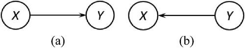
Theoretically, this BN is a mathematical model explaining the joint probability that the variables X and Y have arbitrary realizations x and y, which is written in the form$$P\left(X=x,Y=y\right)=P\left(Y=y|X=x\right)P\left(X=x\right)$$

for the DAG in Figure 1(a) or$$P\left(X=x,Y=y\right)=P\left(X=x|Y=y\right)P\left(Y=y\right)$$for that in Figure 1(b) based on the simple probability multiplication rule covered in introductory statistics courses. If more variables are considered, more possible causal structures may be proposed for the group of variables. Figure 2 illustrates two possible causal structures involving three variables, X, Y, and Z.

Fig. 2 Two DAGs with three nodes.

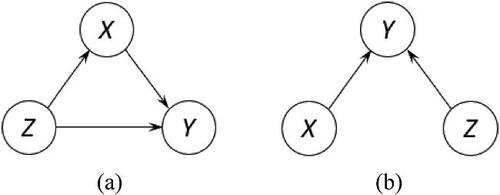
Each causal structure in Figure 2 can be described by a unique mathematical model given their arbitrary realizations x, y, and z,(1) $$\begin{array}{c}\text{Figure} 2(\mathrm{a}):P\left(X=x,Y=y,Z=z\right)=P\left(Y=y|X=x,Z=z\right)\\ \hspace{1em}P\left(X=x|Z=z\right)P\left(Z=z\right)\\ \text{Figure} 2(\mathrm{b}):P\left(X=x,Y=y,Z=z\right)=P\left(Y=y|X=x,Z=z\right)\\ \hspace{1em}P\left(X=x\right)P\left(Z=z\right)\end{array}$$(1) which highlights one essential property of causal inference: it depends on the subjective assumption of causal structure. BNs, thus, provide a mathematical means to describe a causal structure starting from different cause variables and pointing toward the end effect variable.

Having a BN as the mathematical description of causal structure underly a group of variables makes it possible to infer their causal relationships, which is not explicit in empirical data observations. Before introducing BNs as a formal tool for causal inference, we must address a fundamental question: What does causation mean? While a variety of philosophical approaches to causation have been proposed, three approaches closely related to the scope of this study are the probabilistic, counterfactual, and manipulationist approaches.

In the probabilistic approach (e.g., Eells 1991; Mellor 1995; Suppes 1970), causation is defined as the probability of an event Y = y being raised by another event X = x. In other words, the latter is a probabilistic cause of the former just in the case $P(Y=y|X=x)>P(Y=y|X=x^{-})$, where x^– is read as “not x.” However, this approach does not convincingly establish a causal relationship. One primary concern is that the mechanism of probability raising from $P(Y=y|X=x^{-})$ to $P(Y=y|X=x)$ cannot be explained by the classical probability theory (Pearl 2000). As a result, it is hard to distinguish between genuine causation and spurious correlation. Alternatively, Lewis (1973) proposes a counterfactual approach to causation. This approach starts with the premise that both X = x and Y = y occur in the real world, and then, we examine its counterfactual statement: If $X=x\mathit{were}\mathit{not}to\mathit{occur},\mathit{then}Y=y$ would not occur in the most similar world. If the counterfactual statement is true, a cause-effect relationship between x and y can be established. The problem with Lewis’ approach is defining the most similar world and finding evidence there to verify or falsify the counterfactual statement. The manipulationist approach (e.g., Gasking 1955; Menzies and Price 1993) argues that the center of our understanding of causation is, in fact, ourselves. Gasking (1955) notes, “…the notion of causation is essentially connected with our manipulative techniques for producing results…” (p. 483); Menzies and Price (1993) note, “…the ordinary notions of cause and effect have a direct and essential connection with our ability to intervene in the world as agents…” (p. 187). Thus, the best way to determine causation is by human intervention and manipulation whenever such manipulation and intervention is possible, for example, through controlled experiments.

The theory of causal inference unifies the three approaches to causation with Bayesian networks (Pearl 2000). It is not the objective of this article to examine the details of the causal inference theory. Instead, we highlight that the essence of causal inference is well reflected in Bayes’ theorem named after Reverend Thomas Bayes for his pioneering work (Bayes 1763). Suppose it is a reasonable proposal that X = x is a cause of Y = y (as described in Figure 1(a)). For instance, X is the variable of Jen’s behavior; Y is the variable of window condition. Meanwhile, $x:=${Jen throws a ball at a window}and $y:=${the window is broken}. According to Bayes’ theorem, we can express the relationship between X = x and Y = y in the following form(2) $$P\left(X=x|Y=y\right)=\frac{P\left(Y=y|X=x\right)P\left(X=x\right)}{P\left(Y=y\right)}.$$(2)

Mathematically, Equation (2)(2) $$P\left(X=x|Y=y\right)=\frac{P\left(Y=y|X=x\right)P\left(X=x\right)}{P\left(Y=y\right)}.$$(2) is a simple application of the conditional probability formula. In the Bayesian interpretation, $P(X=x)$ measures one’s strength of subjective belief of X = x expressed in probability terms (i.e., $P(X=x)=0$ represents the belief that X cannot take the value x; $P(X=x)=1$ represents the belief that X takes the value x for certain); $P(X=x|Y=y)$ measures this probabilistic belief updated by Y = y. Hence, the significance of Bayes’ theorem is that it provides a formal mathematical rule for transforming human subjectivity into the objectivity of scientific inquiry, which aligns with the manipulationist approach. Further, the marginal probability $P(Y=y)$ is irrelevant in the Bayesian perspective because it is a constant numerical value that does not depend on any pre-condition. Many statistical computation methods take advantage of this Bayesian property (Robert and Casella 2013). This attractive property also makes Bayes’ theorem particularly useful for determining causation, which can be shown as follows.

Analogous to Equation (2)(2) $$P\left(X=x|Y=y\right)=\frac{P\left(Y=y|X=x\right)P\left(X=x\right)}{P\left(Y=y\right)}.$$(2) , we can write(3) $$P\left(X=x^{-}|Y=y\right)=\frac{P\left(Y=y|X=x^{-}\right)P\left(X=x^{-}\right)}{P\left(Y=y\right)}.$$(3)

Following some straightforward mathematical operations on (2) and (3) together, we obtain(4) $$P\left(Y=y|X=x\right)P\left(X=x\right)+P\left(Y=y|X=x^{-}\right)P\left(X=x^{-}\right)=P\left(Y=y\right).$$(4)

Equation (4)(4) $$P\left(Y=y|X=x\right)P\left(X=x\right)+P\left(Y=y|X=x^{-}\right)P\left(X=x^{-}\right)=P\left(Y=y\right).$$(4) implies that we can generate a hypothetical value for $P(Y=y)$, which we denote $P_{\text{hypo}}(Y=y)$, by manipulating $P(X=x)$ and $P(X=x^{-})$. Suppose we deliberately set $P(X=x)=1$ (i.e., make x occur for certain). In that case, $P_{\text{hypo}}{(Y=y)}_{X=x}=P(Y=y|X=x)$. Otherwise, $P_{\text{hypo}}{(Y=y)}_{X=x^{-}}=P(Y=y|X=x^{-})$, if $P(X=x^{-})$ is set to be one (i.e., make x^– occur for certain). That reflects the counterfactual aspect of causation. Finally, following the probabilistic approach, if $P_{\text{hypo}}{(Y=y)}_{X=x}>P_{\text{hypo}}{(Y=y)}_{X=x^{-}}$, we conclude that x is a probabilistic cause of y.

Our introduction only scratches the surface of BNs for causal inference purposes. The readers can refer to the classical literature, Neapolitan (1990) and Pearl (1988), to dig deeper into the richness of this methodology.

2.2 do-Calculus

Our previous manipulation of $P(X=x)$ and $P(X=x^{-})$, that is, deliberately setting their values to be one or zero, is simply an illustration of the intuition behind the more general do-Calculus methodology developed in Pearl (1995, 1994) and later enriched by Valorta and Huang (2006), Shpitser and Pearl (2006), and Tian and Pearl (2002). The do-Calculus methodology has constructed a complete and coherent mathematical framework for causal inference. An in-depth discussion of do-Calculus is beyond the scope of this article. We direct the interested readers to Korb and Nicholson (2010) and Pearl (2009, 2000) for more advanced content on this subject. Next, we explore the intuition behind do-Calculus that can help instructors employ our proposed examples in their classroom.

Pearl and Mackenzie (2018) vividly describe the epistemological nature of causal inference.

Another of his [Mr. Holmes] famous quotes suggest his modus operandi: “When you have eliminated the impossible, whatever remains, however improbable, must be the truth.” Having induced several hypotheses, Holmes eliminated them one by one in order to deduce (by elimination) the correct one (p. 93).

As such, the causal inference appears to involve both induction and deduction. Because of its dependence on deductive reasoning, a causal inference conclusion is inevitably based on the premise of a known “true” causal structure. Consider the causal structure depicted in Figure 1(a) (i.e., X is the cause variable of $Y)$. They note that the induction from an observed effect ($Y=y)$ to its possible cause (X = x or $x^{-})$ is more mysterious and challenging than the deduction from a presumed cause (X = x or $x^{-})$ to its effect ($Y=y)$. They further conclude that the perhaps most important philosophical role of Bayes’ theorem, despite its mathematical simplicity, is “…we can estimate the conditional probability directly in one direction, for which our judgment is more reliable, and use mathematics to derive the conditional probability in the other direction, for which our judgment is rather hazy…” (p. 101). One meaningful takeaway from this philosophical role played by Bayes’ theorem is that the inductive conclusion from effect to cause can be made in the deductive way from cause to effect, which we should prefer because the deduction is more accessible than the induction. In a mathematical sense, to see why deductive reasoning is preferred for causal inference purposes, recall the Bayes’ formula in Equation (2)(2) $$P\left(X=x|Y=y\right)=\frac{P\left(Y=y|X=x\right)P\left(X=x\right)}{P\left(Y=y\right)}.$$(2) . To make the inductive inference of $P(X=x|Y=y)$, we must treat X as a random variable that may require tremendous effort to construct the distribution and domain of X. In contrast, the deductive inference of $P(Y=y|X=x)$ allows us to deliberately assume a known value of $P(X=x)$. Then, the deduction from cause to effect is logically equivalent to the induction from effect to cause. This is because, given a known $P(X=x)$, in the Bayes’ formula the greater $$ implies the greater $P(X=x|Y=y)$ (since the marginal probability $P(Y=y)$ is a constant numerical value).

The question we face now is: How do we know $P(X=x)$? The classical probability theory defines this probability value as the long-run proportion of times the event X = x occurs, so is for $P(X=x^{-})$. But the probabilities of X = x and $X=x^{-}$ estimated by observing their relative proportions of occurrence will not help us make a causal inference. If X is a random variable with multiple possible values and x is only one of the possible values, in the long run, the observed $P(X=x)$ and $P(X=x^{-})$ should be both greater than zero so that they always appear together in Equation (4)(4) $$P\left(Y=y|X=x\right)P\left(X=x\right)+P\left(Y=y|X=x^{-}\right)P\left(X=x^{-}\right)=P\left(Y=y\right).$$(4) to infer the unconditional probability $P(Y=y)$. As such, it is impossible to describe the dynamic of probability changing from $P(Y=y|x^{-})$ to $P(Y=y|x)$, that is, needed for causal inference purposes. Instead, Pearl (1995, 1994) jumps outside the boundary of the classical probability theory and creates a new set of probability rules called do-Calculus. Simply speaking, Pearl’s do-Calculus admits the deliberate action of intervening on a random variable and manipulating its different possible states in such a way that the variable is held constant at one of the possible states; all other states and their associated data evidence are surgically eliminated. That is what we accomplish with $P(X=x)$ and $P(X=x^{-})$ in the previous section.

For a simple illustration of this surgical intervention and manipulation, consider the DAG in Figure 1(a) again. Suppose we are interested in the effect of deliberately setting X = x (we denote $do\left[X=x\right])$ on Y = y. According to Equation (4)(4) $$P\left(Y=y|X=x\right)P\left(X=x\right)+P\left(Y=y|X=x^{-}\right)P\left(X=x^{-}\right)=P\left(Y=y\right).$$(4) , the probability of Y = y resulting from this action can be written in the form(5) $$\begin{array}{c}{P}_{\text{hypo}}{\left(Y=y\right)}_{X=x}=P\left(Y=y|do\left[X=x\right]\right)\\ =P\left(Y=y|X=x\right)P\left(do\left[X=x\right]\right)\\ =P\left(Y=y|X=x\right)\end{array}$$(5) after we adjust $P(do\left[X=x\right])=1$, which means we eliminate all other possible states of X, so $P(X=x)=1$. It is seen from Equation (5)(5) $$\begin{array}{c}{P}_{\text{hypo}}{\left(Y=y\right)}_{X=x}=P\left(Y=y|do\left[X=x\right]\right)\\ =P\left(Y=y|X=x\right)P\left(do\left[X=x\right]\right)\\ =P\left(Y=y|X=x\right)\end{array}$$(5) that $P(Y=y|do\left[X=x\right])$ is readily calculated as the conditional probability $P(Y=y|X=x)$. But it is critical to note that despite having the identical value in Equation (5)(5) $$\begin{array}{c}{P}_{\text{hypo}}{\left(Y=y\right)}_{X=x}=P\left(Y=y|do\left[X=x\right]\right)\\ =P\left(Y=y|X=x\right)P\left(do\left[X=x\right]\right)\\ =P\left(Y=y|X=x\right)\end{array}$$(5) , $P(Y=y|X=x)$ and $P(Y=y|do\left[X=x\right])$ stand for two different conceptions: $P(Y=y|X=x)$ is, in a general sense, the observed probability of Y = y conditional on X = x (e.g., the probability of knee injury of athletes when we observe they wear a newly designed protective gear); $P(Y=y|do\left[X=x\right])$ is the postintervention probability of Y = y after we fix X at x based on the assumption that X is the cause variable and Y is the effect variable (e.g., the probability of knee injury of athletes after they are required to wear the protective gear under the assumption that the gear causally influences the chance of getting the injury). Pearl, Glymour, and Jewell (2016) writes,

When we intervene on a variable in a model, we fix its value. We change the system and the values of other variables often change as a result. When we condition on a variable, we change nothing; we merely narrow our focus to the subset of cases in which the variable takes the value we are interested in (pp. 53–54).

So statistically, the essence of do-Calculus is that under some causal assumption, we deliberately alter the sample space of one random variable to only contain a specific deterministic value and remove all other possible values, and then to see how our action influences the probability of another variable of interest. Hence, Equation (5)(5) $$\begin{array}{c}{P}_{\text{hypo}}{\left(Y=y\right)}_{X=x}=P\left(Y=y|do\left[X=x\right]\right)\\ =P\left(Y=y|X=x\right)P\left(do\left[X=x\right]\right)\\ =P\left(Y=y|X=x\right)\end{array}$$(5) should be read as “based on our causal assumption that X is the cause variable and Y is the effect variable, if we deliberately trim the sample space of X to control (not observe) it to take the value x, the probability of $Y=y$ will change to $P(Y=y|X=x)$ under this assumption,” which is an Actions sentence classified as “causal” in Pearl (2002). In fact, the conditional probability $P(Y=y|X=x)$ observed without any causal assumption can have a much different value from the postintervention probability $P(Y=y|do\left[X=x\right])$ under a specific causal assumption (see Example 3 in the next section for illustration).

For a slightly more complex example, consider the DAG in Figure 2(a). Suppose we argue X = x is a cause of Y = y. To reflect this causal belief, we intervene on node X in the DAG and set it to x, as seen in Figure 3(a). Accordingly, we modify the model form in (1) for this DAG to be$$\begin{array}{c}{P}_{\text{hypo}}{\left(Y=y,Z\right)}_{X=x}=P\left(Y=y,Z|do\left[X=x\right]\right)\\ =P\left(Y=y|Z,X=x\right)P\left(do\left[X=x\right]|Z\right)P\left(Z\right).\end{array}$$

Fig. 3 The DAG with one intervention node.

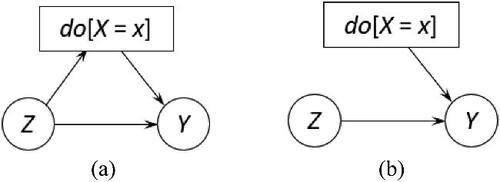
For the sake of simplification, we further assume that our intervention on X should not depend on Z. Thus,$$P\left(Y=y,Z|do\left[X=x\right]\right)=P\left(Y=y|Z,X=x\right)P\left(do\left[X=x\right]\right)P\left(Z\right).$$

The DAG reflecting this additional assumption is given in Figure 3b. (See Example 3 in the next section for an illustration of this independence assumption and Example 5 for the case of dependence structure.)

Then, we obtain$$P\left(Y=y,Z|do\left[X=x\right]\right)=P\left(Y=y|Z,X=x\right)P\left(Z\right).$$

Next, we marginalize out X to calculate$$P\left(Y=y|do\left[X=x\right]\right)=\sum _{Z}P\left(Y=y,Z|do\left[X=x\right]\right)P\left(Z\right).$$

We can follow the same procedure to investigate the other state $X=x^{-}$ and calculate $P(Y=y|do\left[X=x^{-}\right])$. Finally, we only need to compare the two postintervention probabilities to draw a causal conclusion. The difference between the two probability values$$P\left(Y=y|do\left[X=x\right]\right)-P\left(Y=y|do\left[X=x^{-}\right]\right)$$is known as the “causal effect difference” or “average causal effect” (ACE) (Pearl, Glymour, and Jewell 2016). The ACE is defined to deduce the effect of a cause rather than induce the cause of an effect. Because it is conditioned on our deliberate action on X, that is, $do\left[X=x\right]$ and $do\left[X=x^{-}\right]$, we can also make an inductive conclusion that X = x is a probabilistic cause of Y = y if the ACE is calculated to be positive in that the positive ACE value evidently indicates a rise in the probability of Y = y when X is changed from x^– to x by our action.

One meaningful implication of our discussion in this section is the relationship between subjective knowledge and empirical data, and their interactive role in drawing a causal conclusion. Causal inference (based on BNs and do-Calculus) represents plausible prior causal knowledge expressed in some mathematical language, that is, then combined with empirical data to answer causal queries of practical value (Pearl and Mackenzie 2018). As such, in a causal analysis, our prior knowledge plays the central role of constructing a mental model of the unidirectional and dynamic real-world process that we believe produces the data. The data, in turn, help us answer the question of how the process works to produce its outcomes. In such a way, the causal subjectivity, which is graphically represented by DAG and mathematically operates through Pearl’s do-Calculus, does not diminish with the increase in data size. Therefore, interestingly, the purpose of causal inference is less to estimate the true probability of event occurrence (see one illustrative example in the supplementary material), but to understand how our probabilistic belief of some event occurring can be altered by our intervention and manipulation of the constructed causal model given the data we have in hand. If our prior causal knowledge is strong and logically rigorous, only a handful of (or even no) data instances are required to draw a convincing causal conclusion (see Example 4 in the next section for a typical example). Interested readers can refer to Pearl and Mackenzie (2018) for a more detailed discussion of this aspect in a historical context. On the other hand, when our prior knowledge is weak or vague, a large pile of data can help us better construct the causal model through some data-driven search algorithms for causal structure, such as the max-min hill-climbing algorithm (Tsamardinos, Brown, and Aliferis 2006).

In the end, it is worth noting that Pearl’s do-Calculus and causal inference is not the ultimate solution to all causal inquiries. As pointed out above, the causal model is built solely upon the presumption that its underlying causal structure is true, which restricts the model to only solve the problem of causal analysis, not causal discovery. As a result, there is doubt about the wide usefulness of this approach to causal inference in scientific investigations because no consensus exists about the superiority of DAGs (Aronow and Sävje 2020).

3 Five Teaching Examples for Causal Inference

This section presents five examples that instructors can use to teach causal inference in statistics classes at different levels. The five examples are introduced with increasing complexity to show the gradual accumulation of causal inference knowledge. All the examples are built using Netica (Norsys 2021a), a commercial BNs learning software that offers a free version sufficient for teaching and learning purposes. This software is currently built only for the Windows environment. To use it in the MacOS environment, users can install a compatibility layer for running Windows programs that allows Netica to run with full speed and capability (Norsys 2021b). Alternatively, Mac users can download and install a wrapped version of Netica called NeticaMac (Almond 2021). Some other software options work in both Windows and MacOS environments, for example, Bayesia (2021). We recommend Netica because its user-friendly interface and functional design make it particularly suitable for introductory statistics classes (Norsys 2021c). In the supplementary material, we describe the detailed steps to build a BN model in Netica for the five examples. In our experience, students at all levels can implement our examples and many other examples using this tool without technical difficulties. For instructors and students who prefer using open source tools in their classes, we develop a user-friendly R Shiny application that they can use to work out the five examples (https://github.com/AlyeskaBear/Causal-Inference-BNs). This application largely mimics the functionality of Netica in solving our examples.

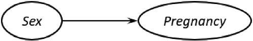
Example 1: Sex as a Cause of Pregnancy

We start with the most unambiguous causal relationship between biological sex (S) and pregnancy (PR) shown in Figure 4.

Fig. 4 The DAG of Example 1.

The model described by this DAG can be directly created in Netica with automatically filled uniform probability values (in percentage point terms) for all states of the two variables, as seen in Figure 5(a).

Fig. 5 Example 1 built in Netica.

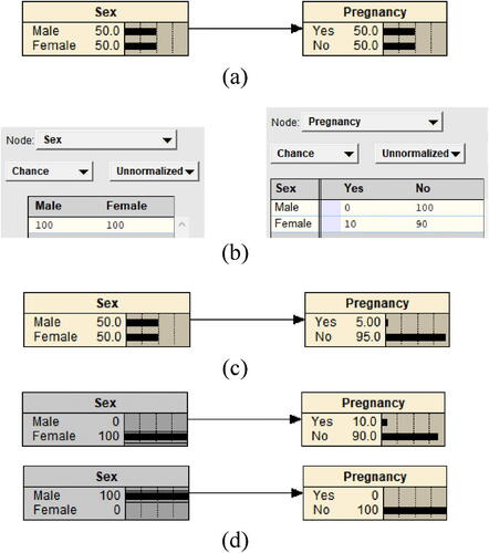
Suppose a simple 2 × 2 frequency table of the two variables is summarized from a fictional group of individuals, as shown in Table 1.

Table 1 The contingency table of Sex and Pregnancy.

		Pregnancy
		Yes	No
Sex	Male	0	100
	Female	10	90

We can load the table data into the nodes Sex and Pregnancy in Netica shown in Figure 5(b). After compiling this model, we obtain the preintervention model output in Figure 5(c). The two output values for the node Pregnancy in this figure are marginal probabilities$$\begin{array}{c}P\left(PR=\text{Yes}\right)=P\left(PR=\text{Yes}|S=\text{Male}\right)P\left(S=\text{Male}\right)\\ \hspace{1em}+P\left(PR=\text{Yes}|S=\text{Female}\right)P\left(S=\text{Female}\right)\\ =0\times 0.5+0.1\times 0.5=0.05\end{array}$$

and$$\begin{array}{c}P\left(PR=\text{No}\right)=P\left(PR=\text{No}|S=\text{Male}\right)P\left(S=\text{Male}\right)\\ \hspace{1em}+P\left(PR=\text{No}|S=\text{Female}\right)P\left(S=\text{Female}\right)\\ =1\times 0.5+0.9\times 0.5=0.95,\end{array}$$as depicted in Equation (4)(4) $$P\left(Y=y|X=x\right)P\left(X=x\right)+P\left(Y=y|X=x^{-}\right)P\left(X=x^{-}\right)=P\left(Y=y\right).$$(4) . To infer the causal effect of sex on pregnancy, we intervene on the node Sex by setting $P(do\left[S=\text{Male}\right])=1$ and $P(do\left[S=\text{Female}\right])=1$ to obtain$$P\left(PR=\text{Yes}|do\left[S=\text{Male}\right]\right)=P\left(PR=\text{Yes}|S=\text{Male}\right)=0$$

and$$P\left(PR=\text{Yes}|do\left[S=\text{Female}\right]\right)=P\left(PR=\text{Yes}|S=\text{Female}\right)=0.1,$$respectively. It is worth noting again that despite being numerically equal, the postintervention probability and the conditional probability are conceptionally distinct in the sense that the former is a consequence of system change; the latter is only a result of observation.

The above theoretical explanation is not necessary when introducing this example in an introductory class. Students can be led to think in such a way that they intervene on this group of people by removing all males (or females) from the group and making it a female (or male) only group. This intuitive intervention and manipulation can be vividly carried out in Netica by setting the percentage of male (or female) to 100% to generate the postintervention model output, as seen in Figure 5(d).

According to our discussion in Section 2.2, the rise in the probability of pregnancy from zero to a positive value evidently indicates that being female in biological sex is one cause of pregnancy.

Example 2: Color Preference by Culture

Many studies have reported cultural differences in color preference. Suppose 100 people with two different cultural ($CU)$ backgrounds, A or B, are surveyed about their color ($C)$ preference. Each survey participant is asked to select their preferred color of black, blue, or red. The survey results are summarized into a two-way contingency table in Table 2.

Table 2 The contingency table of Culture and Color.

		Color
		Black	Blue	Red
Culture	A	25	15	10
	B	5	10	35

The DAG for this example is given in Figure 6.

Fig. 6 The DAG of Example 2.

Following the similar steps as in Example 1, we obtain the preintervention model output as in Figure 7(a). The output values in this figure are marginal probabilities of culture and favored color calculated in the same way as described in Example 1. We then intervene on the variable Culture and set $P(do\left[CU=A\right])=1$ and $P(do\left[CU=B\right])=1$ to obtain $P(C|do\left[CU=A\right])$ and $P(C|do\left[CU=B\right])$. This intervention action can also be explained to students as removing all participants with cultural background A (or B) from the group. Then, we produce the postintervention model output in Netica, as seen in Figure 7(b).

Fig. 7 Example 2 built in Netica.

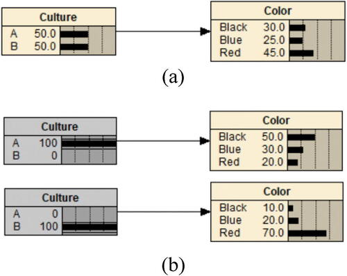
The postintervention probabilities $P(C=\text{Black}|do[CU=B])=0.1$ and $P(C=\text{Black}|do\left[CU=A\right])=0.5$. The rise in the probability of preferring black color from 0.1 to 0.5 provides evidence that having cultural background A, instead of B, is one probabilistic cause of preference for black color.

Example 3: Efficacy of Medication Treatment

Consider a clinical trial in which 80 patients admitted to two different hospitals are randomly given either a newly developed medication or a placebo. The research team wants to answer the question: Does the new medication help recovery of patients? The team collects recovery/no recovery records from patients in the treatment group versus the placebo group. The data are summarized in Table 3.

Table 3 Results of a clinical trial of medication treatment.

	Recovery
Treatment	Yes	No	Recovery Rate
Hospital A (40)
Medication	18	12	60%
Placebo	7	3	70%
Hospital B (40)
Medication	2	8	20%
Placebo	9	21	30%
Combined (80)
Medication	20	20	50%
Placebo	16	24	40%

In this example, we are dealing with three variables: Treatment ($T)$, Hospital ($H)$, and Recovery ($R)$.

As seen from Table 3, this is an example of the renowned phenomenon in statistics, Simpson’s Paradox. In the classical statistical sense, this paradox refers to an arithmetic peculiarity that a relationship between two variables can reverse its sign, depending on whether conditioning on a third variable. In this example, the medication appears to be consistently less effective than the placebo at improving the recovery of patients in each hospital. However, when the trial data are aggregated, the medication is more effective than the placebo.

Figure 8 presents a causal structure that may be argued for this example, in which Recovery is the effect variable and Treatment and Hospital are the two cause variables.

Fig. 8 The DAG of Example 3.

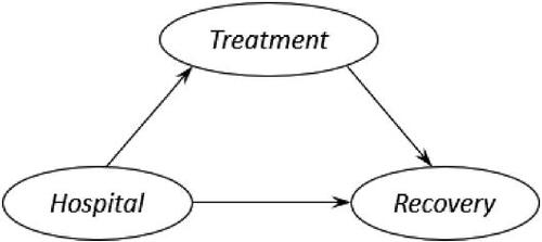
Especially, the edge from Hospital to Treatment is suggested by the data observations that Hospital A patients appear to be more likely than Hospital B patients to receive the medication. This causal structure corresponds to the DAG in Figure 2(a) and is described by the following model$$P\left(R,H,T\right)=P\left(R|H,T\right)P\left(T|H\right)P\left(H\right)$$

In Netica, the preintervention model output conditioned on the causal structure is given in Figure 9(a).

Fig. 9 Example 3 built in Netica.

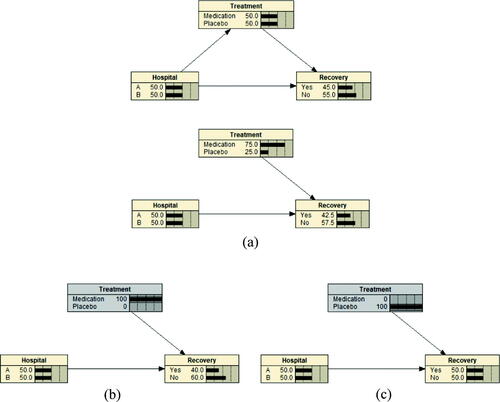
However, this causal structure is not convincing. It assumes hospital is a causing factor of treatment that does not make sense in clinical trial practices. Whether giving a patient medication or placebo in a clinical trial is very unlikely depending on which hospital the patient is admitted to, despite the observed data showing an association between them. Thus, to legitimately infer the causal effect of the medication on patient’s recovery, we must intercept and break off the edge between Hospital and Treatment. This action creates an alternative causal structure shown in Figure 9(b), which corresponds to the DAG in Figure 3(b). The model for this alternative causal structure is given as$$P\left(R,H,T\right)=P\left(R|H,T\right)P\left(T\right)P\left(H\right).$$

Then, we set $P(do\left[T=\text{Medication}\right]) = 1$ and $P(do[\mathrm{}T=\text{Placebo}])=1$, respectively, to obtain$$\begin{array}{c}P\left(R=\text{Yes},H|do\left[T=\text{Medication}\right]\right)\\ \mathrm{\hspace{1em}}\mathrm{\hspace{1em}}=P\left(R=\text{Yes}|H,T=\text{Medication}\right)P\left(H\right)\end{array}$$and$$P\left(R=\text{Yes},H|do\left[T=\text{Placebo}\right]\right)=P\left(R=\text{Yes}|H,T=\text{Placebo}\right)P\left(H\right)$$

By marginalizing out Hospital, we can calculate $P(R=\text{Yes}|do[T=\text{Medication}])$ and $P(R=\text{Yes}|do\left[T=\text{Placebo}\right])$ as following$$\begin{array}{c}P\left(R=\text{Yes}|do\left[T=\text{Medication}\right]\right)\\ \mathrm{\hspace{1em}}\mathrm{\hspace{1em}}=P\left(R=\text{Yes}|H=A,T=\text{Medication}\right)P\left(H=A\right)\\ \hspace{1em}\mathrm{\hspace{1em}}\mathrm{\hspace{1em}}+P\left(R=\text{Yes}|H=B,T=\text{Medication}\right)P\left(H=B\right)\\ \mathrm{\hspace{1em}}\mathrm{\hspace{1em}}=0.6\times 0.5+0.2\times 0.5=0.4\end{array}$$

and$$\begin{array}{c}P\left(R=\text{Yes}|do\left[T=\text{Placebo}\right]\right)\\ \mathrm{\hspace{1em}}\mathrm{\hspace{1em}}=P\left(R=\text{Yes}|H=A,T=\text{Placebo}\right)P\left(H=A\right)\\ \mathrm{\hspace{1em}}\mathrm{\hspace{1em}}\hspace{1em}+P\left(R=\text{Yes}|H=B,T=\text{Placebo}\right)P\left(H=B\right)\\ \mathrm{\hspace{1em}}\mathrm{\hspace{1em}}=0.7\times 0.5+0.3\times 0.5=0.5.\end{array}$$

In Netica, after we set $P(do\left[T=\text{Medication}\right])=1$ and $P(do\left[T=\text{Placebo}\right])=1$, the hospital factor is automatically marginalized out, and the postintervention model output is given in Figure 9(c).

The decline in the probability of recovery from 0.5 to 0.4 makes us conclude that this medication is unlikely to be helpful for patient’s recovery. It is worth highlighting that in Table 3, the observed conditional probability without a causal assumption $P(R=\text{Yes}|T=\text{Medication}) = 0.5$, which is different from the postintervention probability $P(R=\text{Yes}|do[T=\text{Medication}])=0.4$ under our assumption. Hence, causal inference provides a sensible solution to Simpson’s Paradox that we will discuss in more detail in a later section when we provide suggestions on using this example in statistics classes.

Example 4: Should I switch?

This example covers the fascinating tale in probabilistic reasoning: The Monty Hall Problem. Pearl and Mackenzie (2018) describe the most common version of this problem,

Suppose you’re on a game show, and you’re given the choice of three doors. Behind one door is a car, behind the others, goats. You pick a door, say #1, and the host, who knows what’s behind the doors, opens another door, say #3, which has a goat. He says to you, ‘Do you want to pick door #2?’ Is it to your advantage to switch your choice of doors? (p. 190)

To facilitate our discussion below, we call the contestant Jen. The variables of our interest are the door picked by Jen, the door opened by the Host, and the door hiding the Car. Although there are also three variables, as in Example 3, we face a more complex and counterintuitive cause-effect scenario.

The probability relationships among the three variables are given in Table 4.

Table 4 The probability tables of Jen and Car.

Jen
Door 1	Door 2	Door 3
1/3	1/3	1/3
Car
Door 1	Door 2	Door 3
1/3	1/3	1/3

In this case, it is not hard to see that the host’s choice is affected by both Jen’s pick and the door hiding the car. Meanwhile, there should be no relationship between Jen and Car because Jen does not know which door hides the car, and the car will not be moved after it is placed behind one door regardless of which door is picked by Jen. So, a reasonable causal structure for this example is depicted by the DAG in Figure 10, which corresponds to the one in Figure 2(b).

Fig. 10 The DAG of Example 4.

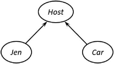
Its corresponding BN model is given as$$P\left(\text{Host},\text{Jen},\text{Car}\right)=P\left(\text{Host}|\text{Jen},\text{Car}\right)P\left(\text{Jen}\right)P\left(\text{Car}\right)$$

After loading the data in Tables 4 and 5 and this DAG into Netica, we can set $\text{Jen}=\text{Door}1$ as their intervention made (i.e., $P(do\left[\text{Jen}=\text{Door}1\right])=1)$ and $\text{Host}=\text{Door}3$ as the observed outcome of the host’s action. The updated DAG and model output in Netica is given in Figure 11(a). It shows that the probability of Door 2 hiding the car is higher than that of Door 1, ironically suggesting the dependence of Car on Jen. A layperson’s explanation of this outcome is that when Jen picks Door 1, they know $P(\text{Car}=\text{Door}1)=1/3$, which should stay unchanged. After the host reveals nothing is behind Door 3, either Door 1 or Door 2 hides the car. Because of $P(\text{Car}=\text{Door}1)=1/3$, it is a must that $P(\text{Car}=\text{Door}2)=2/3$. Alternatively, Bayes’ theorem can be applied to calculate the posterior probabilities of $P(\text{Car}=\text{Door}1|\text{Host}=\text{Door}3)=1/3$ and $P(\text{Car}=\text{Door}2|\text{Host}=\text{Door}3)=2/3$.

Fig. 11 Example 4 built in Netrica.

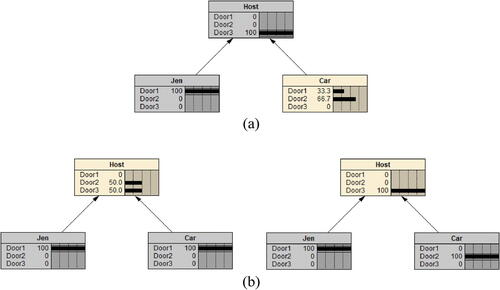
Table 5 The joint probability table of Jen, Car, and Host.

		Host
Jen	Car	Door 1	Door 2	Door 3
Door1	Door 1	0	1/2	1/2
Door 1	Door 2	0	0	1
Door 1	Door 3	0	1	0
Door 2	Door 1	0	0	1
Door 2	Door 2	1/2	0	1/2
Door 2	Door 3	1	0	0
Door 3	Door 1	0	1	0
Door 3	Door 2	1	0	0
Door 3	Door 3	1/2	1/2	0

However, neither the layperson’s explanation nor the Bayesian calculation affords a clear causal argument for this surprising dependence relationship. The argument can be built convincingly by speaking in the do-Calculus language. We write the BN model in Figure 11(a) as$$\begin{array}{c}P\left(\text{Host}=\text{Door}3,\text{Car}|do\left[\text{Jen}=\text{Door}1\right]\right)\\ \mathrm{\hspace{1em}}\mathrm{\hspace{1em}}=P\left(\text{Host}=\text{Door}3|\text{Jen}=\text{Door}1,\text{Car}\right)P\left(\text{Car}\right).\end{array}$$

Our intervention targets the other cause variable Car: We set either $P(do\left[\text{Car}=\text{Door}1\right])=1$ or $P(do\left[\text{Car}=\text{Door}2\right])=1$. Accordingly, we have$$\begin{array}{c}P\left(\text{Host}=\text{Door}3|do\left[\text{Jen}=\text{Door}1\right],do\left[\text{Car}=\text{Door}1\right]\right)\\ \mathrm{\hspace{1em}}\mathrm{\hspace{1em}}=P\left(\text{Host}=\text{Door}3|\text{Jen}=\text{Door}1,\text{Car}=\text{Door}1\right)=\frac{1}{2}\end{array}$$

and$$\begin{array}{c}P\left(\text{Host}=\text{Door}3|do\left[\text{Jen}=\text{Door}1\right],do\left[\text{Car}=\text{Door}2\right]\right)\\ \mathrm{\hspace{1em}}\mathrm{\hspace{1em}}=P\left(\text{Host}=\text{Door}3|\text{Jen}=\text{Door}1,\text{Car}=\text{Door}2\right)=1,\end{array}$$as given in the first and second rows of Table 5. In Netica, we can easily calculate the two postintervention probabilities by intervening on Jen and Car but not on Host, as shown in Figure 11(b).

As discussed previously, after Jen picks Door 1, we trim the sample space of Car to first include Door 1 only, and then only include Door 2. Figure 11(b) illustrates our action’s causal effect on Host: the later raises the probability that the host opens Door 3 from 1/2 to 1. So, a logical conclusion is that Door 2 hiding the car is more likely the reason why the host opens Door 3, and a switch is to Jen’s advantage.

Example 5: Effect of Smoking on Forced Expiratory Volume

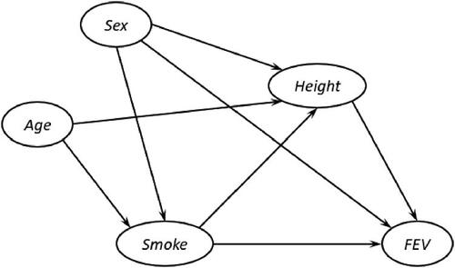
In this example, we revisit the classroom activity introduced in Cummiskey et al. (2020) that studies the effect of Smoke ($SM)$ on forced expiratory volume (liters) (FEV), when several other factors are also taken into consideration, including Age ($A)$, Height ($H)$, and Sex ($S)$. The DAG for this example is given in Figure 12whose BN model is written as$$\begin{array}{c}P\left(\text{FEV},\mathrm{S}M,A,S,H\right)=P\left(\text{FEV}|SM,A,S,H\right)P\left(H|SM,A,S\right)\\ \hspace{1em}P\left(SM|A,S\right)P\left(A\right)P\left(S\right).\end{array}$$

Fig. 12 The DAG of Example 5.

Adapted from “Causal Inference in Introductory Statistics Courses,” by Cummiskey et al. 2020, Journal of Statistics Education, 28, p. 6 under the terms of the Creative Commons CC BY license.

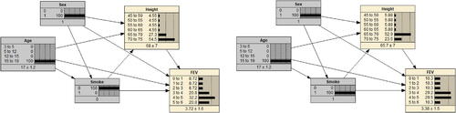
We build the preintervention model in Netica using the same dataset referred to in their article (the dataset fev.dat.txt is publicly available at http://jse.amstat.org/jse_data_archive.htm). It is easy to build a BN model in Netica directly from an empirical data file. For variables with discrete values, Netica will automatically create their probability tables. On the other hand, if one variable has continuous (or approximately continuous) values, we can manually specify the number of buckets for possible values of the variable, and Netica will automatically partition data into the buckets for model compiling. In this example, we define buckets of equal length for each of Height and FEV and four buckets of 3 to 5, 5 to 12, 12 to 15, and 15 to 19 for Age. The resulted preintervention model is presented in Figure 13(a). Instructors can explain to students that discretizing a variable is not required for building a BN model in a theoretically technical sense, just often in a practical sense for building a discrete BN model conventionally using software. For instance, the Gaussian Bayesian Networks can model continuous variables directly (Grzegorczyk 2010).

Fig. 13 Example 5 built in Netica and intervention on Smoke only.

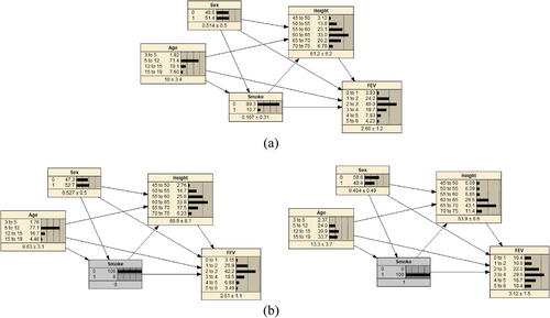
For students, intervention on the cause variable of interest, Smoke, will be more complex than in the previous examples because this variable has two parents, Age and Sex. Figure 13(b) shows the model output after only intervening on Smoke.

In Figure 13(b), we see that switching from Smoke =0 to Smoke =1 pushes the distribution of FEV toward larger values. That might suggest smoking cause an increase in forced expiratory volume, which, however, is not a convincing conclusion as we discuss next.

Mathematically, this intervention action can be expressed as(6) $$\begin{array}{c}P\left(\text{FEV}|do\left[SM=sm\right]\right)\\ \hspace{1em}=\sum _{A,S,H}P\left(\text{FEV}|SM=sm,A,S,H\right)P\left(H|SM=sm,A,S\right)\\ \mathrm{\hspace{1em}}\mathrm{\hspace{1em}}P\left(do\left[SM=sm\right]|A,S\right)P\left(A\right)P\left(S\right)\\ \hspace{1em}=\sum _{A,S,H}P\left(\text{FEV}|SM=sm,A,S,H\right)P\left(H|SM=sm,A,S\right)P\left(A\right)P\left(S\right)\end{array}$$(6) where sm = 0 and 1, respectively. The issue with Equation (6)(6) $$\begin{array}{c}P\left(\text{FEV}|do\left[SM=sm\right]\right)\\ \hspace{1em}=\sum _{A,S,H}P\left(\text{FEV}|SM=sm,A,S,H\right)P\left(H|SM=sm,A,S\right)\\ \mathrm{\hspace{1em}}\mathrm{\hspace{1em}}P\left(do\left[SM=sm\right]|A,S\right)P\left(A\right)P\left(S\right)\\ \hspace{1em}=\sum _{A,S,H}P\left(\text{FEV}|SM=sm,A,S,H\right)P\left(H|SM=sm,A,S\right)P\left(A\right)P\left(S\right)\end{array}$$(6) is that the postintervention distribution of FEV is subject to the action of setting $P(do\left[SM=sm\right]|A,S)=1$, which is not straightforward. As we discussed before, do-Calculus’s statistical essence is to deliberately alter the sample space of a selected variable. Here, because the variable Smoke is statistically conditioned on Age and Sex, our action of trimming its sample space to only contain the value “0” or “1” has a reverse effect on Age and Sex. Also seen in Figure 13(b), switching from no smoking to smoking shifts the distribution of Age toward older ages and the distribution of Sex toward the value “0.” It makes intuitive sense that the prevalence of smoking tends to be higher among those of older age and/or in a particular sex category. Students should quickly understand that this effect is non-causal because smoking apparently cannot change one person’s age or sex category. However, this effect introduces a spurious relationship between Smoke and FEV due to the causal effects of Age and Sex on FEV, as shown in Figure 14(a).

Fig. 14 The spurious relationship between Smoke and FEV in Example 5.

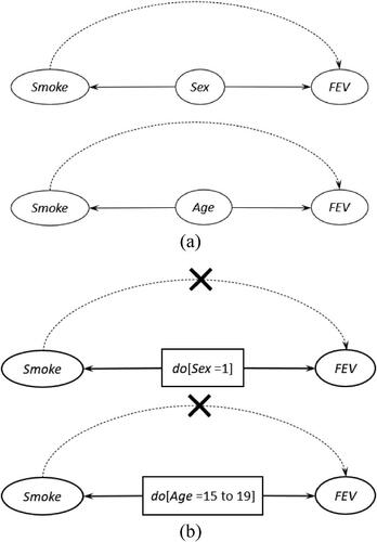
As such, the change in forced expiratory volume caused by age and/or sex will appear to be due to smoking. Therefore, to properly infer the causal effect of smoking on forced expiratory volume, we must remove their spurious relationship.

Figure 14(a) suggests that to remove the spurious relationship, we need to further intervene on both Sex and Age to fix their values so that the paths from Smoke to FEV through the two variables are blocked. For instance, we can set $\text{Sex}=1$ and $\text{Age}=15\text{to}19$ shown in Figure 14(b). The postintervention model output is given in Figure 15.

Fig. 15 Example 5 built in Netica and intervention on Smoke, Age, and Sex.

Its mathematical expression is given as$$\begin{array}{c}P\left(\text{FEV}|do\left[SM=sm,A=15\text{to}19,S=1\right]\right)\\ \hspace{1em}=\sum _{H}P\left(\text{FEV}|SM=sm,A=15\text{to}19,S=1,H\right)\\ \mathrm{\hspace{1em}}\mathrm{\hspace{1em}}P\left(H|SM=sm,A=15\text{to}19,S=1\right)\\ \times P\left(do\left[SM=sm\right]|A=15\text{to}19,S=1\right)P\left(do\left[A=15\text{to}19\right]\right)\\ \mathrm{\hspace{1em}}\mathrm{\hspace{1em}}P\left(do\left[S=1\right]\right)=\sum _{H}P\left(\text{FEV}|SM=sm,A=15\text{to}19,S=1,H\right)\\ \mathrm{\hspace{1em}}\mathrm{\hspace{1em}}P\left(H|SM=sm,A=15\text{to}19,S=1\right)\end{array}$$

It is seen in Figure 15 that switching from Smoke =0 to Smoke =1 pushes the distribution of FEV toward lower values. So, we conclude that smoking can reduce forced expiratory volume. Students may ask why we do not intervene on Height. The reason is that in our proposed causal structure, Height is a child node of Smoke as seen in Figure 16 and thus does not introduce a spurious relationship between Smoke and FEV as the other two variables do.

Fig. 16 The causal relationship between Smoke and FEV through Height in Example 5.

4 Suggestions on Using the Five Examples in the Classroom

Based on our experience teaching causal inference to students, we provide some suggestions in this section on using the five demonstrative examples in statistics classes at different levels.

The earliest possible moment students can wonder about the cause-effect relationship between variables is when they learn the concept of conditional probability with a simple 2 × 2 frequency table. When learning this concept, in our experience, many students have the misconception that a higher (or lower) value of $P(X=x|Y=y)$ necessarily implies a higher (or lower) value of $P(Y=y|X=x)$. One good example we use to illustrate the falsehood of this conception is to define X to be the variable of a random person’s biological sex with possible realizations $x_1:=${Female}and $x_2:=${Male}, and define Y to be the variable of pregnancy test result (assuming the test accuracy is 100%) with possible realizations $y_1:=${Pregnant}and $y_2:=${Not Pregnant}. Students will quickly see that in this case, $P(X=x_1|Y=y_1)=1$ but $P(Y=y_1|X=x_1)$ is much lower than one, in contrast, $P(X=x_2|Y=y_1)=P(Y=y_1|X=x_2)=0$. We suggest that instructors first use this or another similar enlightening example to help students be aware of the difference between $P(X=x|Y=y)$ and $P(Y=y|X=x)$. Their understanding of the difference will open the door for them to learn causal inference because they are convinced that inference on a relationship between two variables can be different, depending on the direction of the relationship (from X to Y versus from Y to $X)$. Then instructors can present Example 1 to students as a hypothetical do-Calculus experiment in Netica focusing on the directional relationship from sex to pregnancy, which is also an introduction to the software.

Example 2 closely follows Example 1 and can be presented to students after instructors extend the simple 2 × 2 frequency table to the more general case of a two-way contingency table. The essential difference between the two examples is that Example 1 illustrates an intuitive deterministic causal relationship between two variables; Example 2 is a simple demonstration of probabilistic cause in causal inference. In other words, in Example 2, we conclude whether the occurrence of a cause increases the probability of its effect (Borgelt and Kruse 2002). This example is still simple in the sense that the causal relationship between culture and color preference is clear and easy to understand: culture is the cause variable, and color preference is the effect variable.

GAISE II states, “…Level B students should understand that contingency tables can also be used to discuss probabilities, especially joint and conditional probabilities…” (American Statistical Association 2020, p. 52). Examples 1 and 2 require only a basic understanding of conditional probability and two-way contingency table. Also, the two examples represent the simplest causation scenario that involves only one causal variable and one effect variable. According to our experience, students can understand a visual depiction of the causal relationship between variables in the two examples, as shown in Figures 4 and 9, without formally being introduced to the concept of DAG. Hence, the two examples can serve as an informal introduction of causal inference in an introductory course at the K-12 level to help level B students develop their initial understanding of causality and causal inference.

In later college-level statistics courses, instructors often present Simpson’s paradox as a curiosity when students learn the concept of the three-way contingency table. Many examples of this statistical phenomenon have been circulating in the community of statistics instructors. Different from most, if not all, of the existing examples, Example 3 illustrates how this paradox can be solved under the framework of causal inference. A similar example is also discussed in Barber (2012, p. 48), but we present it in a way that does not involve deep theoretical discussion. When leading classroom discussion on this example, an instructor must first explain to students what “solving” Simpson’s paradox means when phrased as a causal inference problem. According to Pearl (2014) and Pearl, Glymour, and Jewell (2016), to solve Simpson’s paradox and any other causal inference problem in general, we ought to make two fundamental causal assumptions. First, a causal inference problem must be framed and solved based on a preexisting causal structure as stated in Pearl (2000), “…unless one knows in advance all causally relevant factors or unless one can carefully manipulate some variables, no genuine causal inferences are possible” (p. 42). Second, with a presumed causal structure, to infer a genuine causal relationship between a cause variable and its effect variable, we must intercept any path between the two variables that we “believe” carry a spurious relationship. Apparently, it is impossible, at least practically impossible, to thoroughly test the two assumptions by empirical data observations, and thus they are subjective in their nature. In our example, we start with the causal structure encoded by the DAG in Figures 8 and 9(a). However, the reasonable belief is that in a clinical trial, the decision of giving medicine or placebo to a patient as treatment is very unlikely depending on which hospital the patient is admitted to. Hence, the dependence of treatment on hospital embodied in this causal structure, even though supported by the data observations, introduces a spurious relationship between treatment and patient’s recovery. We intercept the path from hospital to treatment to prevent this spurious relationship by removing the edge between the two variables.

Consequently, solving this Simpson’s paradox problem should be based on the causal structure encoded by the DAG in Figure 9(b). Under this causal structure, we calculate $P(R=\text{Yes}|do\left[T=\text{Medication}\right]) = 0.4$, in contrast to the ob- served conditional probability $P(R=\text{Yes}|T=\text{Medication})=0.5$ without assuming a causal structure. This example is purposely aimed to help students build their first impression of causal assumption as one essential building block of causal inference, simply, no causes (the assumption) in—no causes (the conclusion) out (Cartwright 1989).

Example 4 is focused on a renowned mathematical brain teaser as well. We suggest that this example be used as one classroom exercise in a more advanced statistics course in which Bayes’ theorem and related concepts, including prior and posterior probabilities, are formally introduced. This exercise is for students to practice the four basic steps in solving a causal inference problem:

• Step 1: Determine the cause and effect variables.

• Step 2: Propose a DAG to describe the variables’ causal structure.

• Step 3: Complete the probability tables as seen in Table 4.

• Step 4: Make causal inference based on data evidence from some intervention and manipulation actions on the cause variable(s).

In our experience, it is helpful to reveal to students the correct answer to the Monty Hall problem before assigning this exercise because the answer key implies dependence between Jen’s pick and which door hides the car. As a result, students will likely struggle with deciding the relationship between the two variables in the first and second steps. That creates an opportunity for instructors to highlight the relevance of the second causal assumption we mention above and lead students to discuss the spurious nature of the association between two variables because of conditioning on a third variable. In essence, a realization of the third variable limits possible values one or both variables can take, which are now constrained by the realized value. For instance, the car can only be hidden behind Door 1 or 2 after the host opens Door 3. So, this example is also a demonstration of the essential role of probabilistic reasoning in causal inference.

When the third step is relatively straightforward, students often need help to fully understand the distinction between the causal inference made in the last step and the statistical inference based on posterior probabilities derived from Bayes’ theorem. Their principal difference is that Bayesian posterior probability is inductive evidence allowing people to infer the possible cause (which door hides the car) directly from the observed effect data (the host opens Door 3). On the contrary, causal inference is made in Mr. Holmes’ way of deductive thinking. That is that we fix the cause variable at its two possible states (Door 1 or Door 2) separately under our presumed causal structure and investigate the probability of each state producing the observed effect of Door 3 being opened by the host. As discussed in Section 2.2, this deductive way of making a causal inference is preferable.

After completing Example 4, students are expected to develop a basic understanding of the mechanism of causal inference. For students who want to learn advanced content on this subject, such knowledge prepares them to grasp more theoretical concepts in their future studies. For instance, the causal structure proposed for Jen, Car, and Host illustrates the concept of Collider, one of the three fundamental causal graph structures. For many other students, these examples prepare them to learn how to implement causal inference to solve some real-world problems. In this regard, our last example illustrates practical applications of causal inference.

Although Example 5 rests on a more complicated causal structure than the other examples, instructors can lead students to see that this causal structure consists of seven triangular substructures as shown in Figure 17, which can also be related to Figure 8 for Example 3.

Fig. 17 The triangular substructures of the DAG of Example 5.

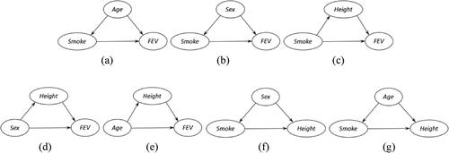
As a result, students will foresee the need to intercept some paths carrying a spurious relationship in the substructures, as we discussed above for Example 3. Also, without knowing the concept of backdoor criterion, they can recognize the paths that require interception (in Figure 17(a) and (b)) by thinking in this way. But our treatment of spurious association in this example is different from that in Example 3. Instead of removing the edges from Age and Sex to Smoke, we intercept the paths by fixing the two variables at their selected states. This example is particularly meaningful because it introduces students to the other two fundamental causal graph structures, Fork shown in Figure 14(a) and Chain shown in Figure 16. It is also helpful that instructors compare our causal inference solution to Example 5 with the statistical inference solution presented in Cummiskey et al. (2020). In our solution, closely following the presumed causal structure in Figure 12, we directly infer the causal effect of Smoke on FEV after blocking all the non causal paths between the two variables in the structure. Their solution, conditioned on the observed data, concludes the association between Smoke and FEV after adjusting for Age and Sex. But the causal structure is not a required element of the statistical solution. In consequence, students can better understand the distinction between the two types of scientific inquiry.

In summary, Examples 3 to 5 can be introduced to students in more advanced courses. Example 3 highlights the importance of causal assumption in causal inference; Example 4 further emphasizes the critical role of probabilistic reasoning in causal inference. Finally, Example 5 demonstrates the real-world application of causal inference. In addition, Examples 4 and 5 also illustrate the three fundamental causal graph structures.

We have used Examples 1 and 2 to teach first-year college students in an introductory service statistics course. The course is also open to high school students enrolled in an Advanced Placement program. Example 3 has been used to teach an applied data analysis course enrolling third-year business students majoring in marketing and finance. We have used Example 4 in a decision analytics course for students in a graduate business program; Example 5 was recently introduced into this graduate course. All examples have been received well by students at each level.

5 Concluding Remarks

This article recommends using Bayesian networks and do-Calculus to introduce students to causal inference. Based upon this recommendation, we propose an instructional approach that has several attractive features, including requiring less prerequisite knowledge of statistics, addressing the central question in causal inference, and revealing the relevance and distinction between causal and statistical inference. Moreover, this approach can be consistently implemented in classes at different levels using the same tool and probabilistic language. To facilitate adopting this approach to teaching causal inference, we provide instructors with five demonstration examples that can be used in their classroom. All our examples are built as interactive graphical models, which are fun for students to engage in classroom discussions. The five examples are aimed to help them develop their initial understanding of causality and causal inference (Examples 1 and 2), highlight the difference between causal and statistical inference, and motivate them to learn more concepts for causal inference in the future (Examples 3, 4, and 5), and makes them familiar with real-world applications of causal inference (Example 5).

While these examples are designed to serve different purposes, the main takeaway from all the examples is the relevance and distinction between causal and statistical inference. Both types of scientific inference are conditioned on empirical data observations. According to Box (1976), statistical inference should be an iterative reasoning process involving deduction and induction. But many statistical techniques focus on induction from specific instances to a general conclusion arguing for the generality of a hypothesis or model. Causal inference is essentially a deductive endeavor and has the deductive spirit of concluding about specific instances by following some general premises. As illustrated in all five examples, under a presumed causal structure, the causal modeling determines and compares different likelihoods of some realization of the effect variable after we deliberately intervene on and manipulate a cause variable to restrict it to take some deterministic value.

Supplementary Materials

The supplementary material includes a brief instruction on using Netica to create Bayesian networks models.

References

- Adams, B., Baller, D., Jonas, B., Joseph, A. C., and Cummiskey, K. (2021), “Computational Skills for Multivariable Thinking in Introductory Statistics,” Journal of Statistics Education, 29, 123–131.
- Almond, R. (2021), “Tutorial: Bayesian Networks in Educational Assessment,” available at https://pluto.coe.fsu.edu/BNinEA/NCMETutorial. Accessed on March 10, 2021.
- American Statistical Association (2020), Pre-K–12 Guidelines for Assessment and Instruction in Statistics Education II (GAISE II), Alexandria, VA: American Statistical Association. Available at https://www.amstat.org/asa/files/pdfs/GAISE/GAISEIIPreK-12/textunderscoreFull.pdf.
- Aronow, P. M., and Sävje, F. (2020), “The Book of Why: The New Science of Cause and Effect,” Journal of the American Statistical Association, 115, 482–485. DOI: 10.1080/01621459.2020.1721245.
- Bang-Jensen, J., and Gutin, G. Z. (2008), Digraphs: Theory, Algorithms and Applications. New York: Springer Science & Business Media.
- Barber, D. (2012), Bayesian Reasoning and Machine Learning, Cambridge, UK: Cambridge University Press.
- Bayes, T. (1763), “LII. An Essay towards Solving a Problem in the Doctrine of Chances,” Philosophical Transactions of the Royal Society of London, 53, 370–418.
- Bayesia (2021), “Bayesia,” Available at https://www.bayesia.com/. Accessed on March 10, 2021.
- Borgelt, C., and Kruse, R. (2002), Graphical Models: Methods for Data Analysis and Mining, New York: Wiley.
- Box, G. E. (1976), “Science and Statistics,” Journal of the American Statistical Association, 71, 791–799. DOI: 10.1080/01621459.1976.10480949.
- Cartwright, N. (1989), Nature’s Capacities and Their Measurement, Clarendon Press, Oxford.
- Carver, R., Everson, M., Gabrosek, J., Horton, N., Lock, R., Mocko, M., Rossman, A., Rowell, G., Velleman, P., Witmer, J., and Wood, B. (2016), “Guidelines for Assessment and Instruction in Statistics Education: College Report 2016,” American Statistical Association. Available at https://www.amstat.org/docs/default-source/amstat-documents/gaisecollege/textunderscorefull.pdf.
- Cummiskey, K., Adams, B., Pleuss, J., Turner, D., Clark, N., and Watts, K. (2020), “Causal Inference in Introductory Statistics Courses,” Journal of Statistics Education, 28, 2–8. DOI: 10.1080/10691898.2020.1713936.
- Dawid, A. P. (2002), “Influence Diagrams for Causal Modelling and Inference,” International Statistical Review, 70, 161–189. DOI: 10.1111/j.1751-5823.2002.tb00354.x.
- Eells, E. (1991), Probabilistic Causality. Cambridge: Cambridge University Press.
- Gasking, D. (1955), “Causation and Recipes,” Mind, LXIV, 479–487. DOI: 10.1093/mind/LXIV.256.479.
- Grzegorczyk, M. (2010), “An introduction to Gaussian Bayesian Networks,” in Systems Biology in Drug Discovery and Development, Berlin: Humana Press, pp. 121–147.
- Hernán, M. A., Hsu, J., and Healy, B. (2019), “A Second Chance to Get Causal Inference Right: A Classification of Data Science Tasks,” CHANCE, 32, 42–49. DOI: 10.1080/09332480.2019.1579578.
- Kaplan, D. (2018), “Teaching Stats for Data Science,” The American Statistician, 72, 89–96. DOI: 10.1080/00031305.2017.1398107.
- Korb, K., and Nicholson, A. (2010), Bayesian Artificial Intelligence, Boca Raton, FL: Chapman and Hall/CRC.
- Lauritzen, S. L., and Sheehan, N. A. (2003), “Graphical Models for Genetic Analyses,” Statistical Science, 18, 489–514. DOI: 10.1214/ss/1081443232.
- Lewis, D. (1973), “Causation,” The Journal of Philosophy, 70, 556–567. DOI: 10.2307/2025310.
- Lübke, K., Gehrke, M., Horst, J., and Szepannek, G. (2020), “Why We Should Teach Causal Inference: Examples in Linear Regression with Simulated Data,” Journal of Statistics Education, 28, 133– 139. DOI: 10.1080/10691898.2020.1752859.
- Mellor, D. H. (1995), The Facts of Causation, London: Routledge.
- Menzies, P., and Price, H. (1993), “Causation as a Secondary Quality,” The British Journal for the Philosophy of Science, 44, 187–203. DOI: 10.1093/bjps/44.2.187.
- Neapolitan, R. E. (1990), Probabilistic Reasoning in Expert Systems, New York: Wiley.
- Norsys (2021a), “Netica Application,” Available at https://www.norsys.com/netica.html. Accessed on March 10, 2021.
- Norsys (2021b), “FAQs on Running Windows Programs on a Mac,” Available at https://www.norsys.com/Netica/textunderscoreon/textunderscoreMacOSX.htm. Accessed on March 10, 2021.
- Norsys (2021c), “Netica Tutorial,” Available at https://www.norsys.com/tutorials/netica/nt/textunderscoretoc/textunderscoreA.htm. Accessed on March 10, 2021.
- Pearl, J. (1988), Probabilistic Reasoning in Intelligent Systems: Networks of Plausible Inference, San Mateo, CA: Morgan Kaufmann Publishers Inc.
- Pearl, J. (1994), “A probabilistic calculus of actions,” in Uncertainty in Artificial Intelligence, ed. R. Lopez de Mantaras and D. Poole. San Mateo, CA: Morgan Kaufmann, pp. 452–462.
- Pearl, J. (1995), “Causal Diagrams for Empirical Research,” Biometrika, 82, 669–688.
- Pearl, J. (2000), Causality: Models, Reasoning and Inference, Cambridge, UK: Cambridge University Press.
- Pearl, J. (2002), “Reasoning with Cause and Effect,” AI Magazine, 23, 95–112.
- Pearl, J. (2009), “Causal Inference in Statistics: An Overview,” Statistics Surveys, 3, 96–146.
- Pearl, J. (2014), “Comment: Understanding Simpson’s Paradox,” The American Statistician, 68, 8–13.
- Pearl, J., Glymour, M., and Jewell, N. P. (2016), Causal Inference in Statistics: A Primer, New York: John Wiley & Sons.
- Pearl, D. K., and Lesser, L. M. (2021), “Statistical Edutainment That Lines up and Fits,” Teaching Statistics, 43, 45–51. DOI: 10.1111/test.12241.
- Pearl, J., and Mackenzie, D. (2018), The Book of Why: The New Science of Cause and Effect, New York: Basic Books.
- Ridgway, J. (2016), “Implications of the Data Revolution for Statistics Education,” International Statistical Review, 84, 528–549. DOI: 10.1111/insr.12110.
- Robert, C. P., and Casella, G. (2013), Monte Carlo Statistical Methods, New York: Springer Science & Business Media.
- Shpitser, I., and Pearl, J. (2006), “Identification of Joint Interventional Distributions in Recursive Semi-Markovian Causal Models.” in Proceedings of the National Conference on Artificial Intelligence. Menlo Park, CA: AAAI Press, pp. 1219–1226.
- Suppes, P. (1970), A Probabilistic Theory of Causality, Amsterdam: North-Holland Publishing Company.
- Tian, J., and Pearl, J. (2002), “A General Identification Condition for Causal Effects,” in Proceedings of the Eighteenth National Conference on Artificial Intelligence, Menlo Park, CA: AAAI Press/the MIT Press, pp. 567– 573.
- Tsamardinos, I., Brown, L. E., and Aliferis, C. F. (2006), “The Max-min Hill-climbing Bayesian Network Structure Learning Algorithm,” Machine Learning, 65, 31–78. DOI: 10.1007/s10994-006-6889-7.
- Valorta, M., and Huang, Y. (2006), “Pearl’s Calculus of Intervention is Complete,” in Proceedings of the 22nd Conference on Uncertainty in Artificial Intelligence, Corvallis, OR: AUAI Press, pp. 217–224.