Preparing Students for the Future: Extreme Events and Power Tails

Abstract

We provide tools for identification and exploration of data with very large variability having power law tails. Such data describe extreme features of processes such as fire losses, flood, drought, financial gain/loss, hurricanes, population of cities, among others. Prediction and quantification of extreme events are at the forefront of the current research needs, as these events have the strongest impact on our lives, safety, economics, and the environment. We concentrate on the intuitive, rather than rigorous mathematical treatment of models with heavy tails. Our goal is to introduce instructors to these important models and provide some tools for their identification and exploration. The methods we provide may be incorporated into courses such as probability, mathematical statistics, statistical modeling or regression methods. Our examples come from ecology and census fields. Supplementary materials for this article are available online.

Keywords:

• Extreme events
• Heavy tail distribution
• Law of large numbers
• Power law distribution

1 Introduction

In this work we argue that if we want the new generation of statisticians and data scientists to contribute to the current science and engineering, they should be introduced to models for phenomena with larger than usual variability. When we talk about variability, we think of the volatility rather than variance. Since volatility is expressed in the tails of statistical models and data, we call such models and data “heavy tailed” in this article. To contribute, our graduates will need a good working knowledge of the tools of the trade essential for working with heavy tailed data. In turn, having such tools in their toolbox will add to their employment opportunities.

To be sure, we are not talking about esoteric, exotic, or rarely seen data from processes that do not impact our lives. On the contrary, the heavy tailed phenomena impact our health, safety, economy, as well as the ecology and the environment. There are many examples of data requiring models with heavy tails. Indeed, consider this partial listing of data with heavy tails: the magnitude of earthquakes, the size of landslides or mountain collapses, size of wild fires, hurricane losses, solar flares, heavy rain events, health care costs, the size of financial returns, losses from market crashes, sales for movies, books, or pharmaceuticals, intensity of terrorist attacks, phone and internet traffic, web site hits, network degrees and delays, the number of lives lost in wars, the occurrence of family names, city sizes, firm sizes, and musical fame (e.g., Greiner, Jobmann, and Lipsky 1999; Girvan and Newman 2002; Reed and Hughes 2002; Sornette 2003, 2004; Newman 2005; Jeske and Chakravartty 2006; Clauset, Shalizi, and Newman 2009; Gabaix 2009; Malevergne, Saichev, and Sornette 2013; Schluter and Trede 2018; Gustar 2020, and the references therein). It is important to note that the literature on heavy tailed statistical models is largely in physics, geophysics, seismology, hydrology, climate, finance, and economics outlets. This diversification of the publication venues and information sources provides solid evidence of the overall importance and practical need for the heavy tailed models in all the sciences and engineering.

Further, the objectives of analysis of heavy tailed data are different from the exploration of the “typical” behavior, which is the main focus of the current statistics curriculum. Indeed, we are interested in the events in the tails of a distribution, the extreme events. The reason for this is that the very large or “extreme” events have the most dramatic impact on our lives, health, safety, and the economy, which is why they are studied by researchers in many diverse areas where the information about the size and frequency of “large” events for highly volatile processes is of primary importance.

In addition to the practical need to model data with heavy tails, there are interesting, even surprising, statistical properties of such data. Some of the common tools and methodologies do not work for heavy tailed data. For example, consider data that do not seem to follow Law of Large Numbers (LLN). The common use of the historical mean to predict future observations is unreliable (if the tail is heavy enough). It is therefore important to be able to recognize that a dataset may be coming from a heavy tailed distribution.

While we only address continuous heavy tailed models in this work, several discrete heavy tail models are available to model counts data. Some references for discrete heavy tailed models are provided in the Appendix.

This article is primarily addressed to those teaching probability, mathematical statistics, statistical modeling, or data science courses in the undergraduate (and beginning graduate) level. Statistics methods courses taught in ecology, business, climate science or social sciences may also benefit from the examples and tools presented in this work. While we do not aim at a comprehensive treatment of heavy tailed data and models, we want to bring heavy tail modeling to the attention of teachers and students of statistics and data science.

2 Modeling Heavy Tailed Data

In this section we present two datasets that may serve as class examples. The R code and data we used for the examples are included in the supplementary materials. On September 16, 2020 the Los Angeles Times in “The worst fire season ever. Again” reported that The last 10 years have shattered records. 2020 tops them all…. with 3.2 million acres burned so far. We analyze the last 20 years of the monthly acreage burnt per fire in the United States (for substantial fires defined as those exceeding 200 burnt acres), and show that the data are heavy tailed. Our other example is from the census information collected in 2020. The U.S. Census Bureau (USCB) informs: As mandated by the U.S. Constitution, our nation gets just one chance each decade to count its population. The U.S. census counts every resident in the United States. We shall use USCB estimates of the 2019 population of the U.S. cities with over 250,000 population (based on the 2000 census data) to show that their population follows a heavy tailed distribution. The fact that the data come from heavy tailed populations has direct impact on the estimated resource needs for health, safety, and well-being of people and the environment for many U.S. communities. Our focus is on providing easy to use and understand tools for recognizing heavy tail datasets. We base this section on the exposition in Cooke, Nieboer, and Misiewicz (2014), Newman (2005), and Clauset, Shalizi, and Newman (2009).

We consider two datasets: (a) “FIRES” data, which provide monthly acreage burnt per fire in the United States from January 2000 to October 2020 in fires that burnt at least 200 acres. The data come from the National Interagency Fire Center and was downloaded from the National Oceanic and Atmospheric Administration’s National Climatic Data Center,¹ and (b) “CITIES” data, which provide the size of the U.S. cities (over 250k population) estimated for 2019 using the data from the 2000 Census.²

While “heavy tail” may have different meaning for different statisticians or scientists, in this work we focus our attention on the heavy tailed models with a power law survival function. A random variable X is called heavy tailed if its survival function behaves like a power of x at infinity. That is, we have $\mathbb{P}(X>x)\sim C{x}^{-\alpha }\text{as}x\to \infty$. It follows that for large x, we have: (1) $$\hspace{0.17em}\log \hspace{0.17em}(\mathbb{P}(X>x))\approx \hspace{0.17em}\log \hspace{0.17em}(C)-\alpha \hspace{0.17em}\log \hspace{0.17em}(x).$$(1)

This means that for large values of x, the logarithm of the survival function behaves like a linear function of the log of x. The parameter α is often called the “tail index,” as it provides information on the “heaviness” of the tail of the distribution of X. Indeed, the smaller the α the heavier the tail, that is the larger the (right) tail probability in the asymptotic sense. It is easy to check that moments of order larger than or equal to α do not exist for the heavy tailed random variables with tail index α. It follows that random variables with $\alpha \le 1$ do not have finite mean and those with $\alpha \le 2$ do not have finite variance.

Although we focus on power laws, there are many other distributions that are sometimes also considered heavy tailed (as their tails are heavier than those of the exponential distribution), like the familiar lognormal, Student-t, or Weibull (with shape parameter less than 1) models. Two common and rich sources of heavy tailed models are the Peak-Over-Threshold (POT) and the Extreme Value Theory (EVT), which study the behavior of the maxima (EVT) and exceedences over (high) thresholds (POT). The models coming out of the POT and EVT include several interesting and useful distributions such as Fréchet and Generalized Pareto. Both POT and EVT are focused on the extreme or large events, and estimation of their probabilities. We direct those interested in learning more about EVT and POT to Coles, 2001 and other references mentioned in the Appendix.

We now move to discussion of the tools for recognizing heavy tailed data. We present graphical means of studying such data as these are very popular in the science literature. The three types of plots we include in this article are: (a) the histogram, (b) the log-log empirical survival function plot (LLESF), and (c) the moving average plot. The histograms of both FIRES and CITIES data are strongly skewed to the right and span several orders of magnitude, which is indicative of heavy tails (see Figures 1 and 2, left panels).

Fig. 1 FIRES data: Histogram (the left panel) and LLESF plot (the right panel).

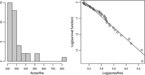
Fig. 2 CITIES data: Histogram (the left panel) and LLSEF plot (the right panel).

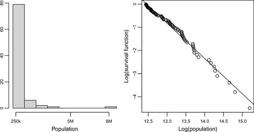
Consistent with the graphical information, the summary statistics show the largest observations being larger than the means or 75th percentiles by several orders of magnitude. Further, the mean (698,070) of the CITIES data exceeds the 75th percentile (670,820), suggesting a very strong skewness (with the maximum value of 8,336,817).

The next step is to check if the power law model fits the data reasonably well. Typically, we start this analysis with a log-log plot of the empirical survival function. Given a random sample $X_1,X_2,\dots ,X_n$, we can graph an “empirical” version of Equation (1)(1) $$\hspace{0.17em}\log \hspace{0.17em}(\mathbb{P}(X>x))\approx \hspace{0.17em}\log \hspace{0.17em}(C)-\alpha \hspace{0.17em}\log \hspace{0.17em}(x).$$(1) and use the linear relationship between $\hspace{0.17em}\log \hspace{0.17em}(\mathbb{P}(X>x))$ and $\hspace{0.17em}\log \hspace{0.17em}(x)$ to estimate the slope $-\alpha$ and the intercept $b=\hspace{0.17em}\log \hspace{0.17em}(C)$. The empirical survival function $\widehat{S}(x)$ is defined as $$\widehat{S}(x)=\frac{\#\mathrm{ }\text{of}\mathrm{ }\text{observations}\mathrm{ }\text{larger}\mathrm{ }\text{than}\mathrm{ }x}{n},\mathrm{ }\text{for}\mathrm{ }x\in \mathbb{R}.$$

Although we plot the entire datasets on the LLESF plots, for the heavy tail data, the $\hspace{0.17em}\log \hspace{0.17em}(S(x))$ does not need to be a linear function of $\hspace{0.17em}\log \hspace{0.17em}(x)$ for all x, but only for large x. Figures 1 and 2 (the right panels) present the LLESF plots of the FIRES and CITIES data, respectively.

Both LLESF plots are relatively straight, signaling that the power tail models fit the distribution of these data reasonably well. The LLESF plots are also useful in estimating the tail parameter α and the intercept $b=\hspace{0.17em}\log \hspace{0.17em}(C)$ using standard regression equation estimation process. For the FIRES data, we obtained $\widehat{\alpha }=3.43$ and the intercept $\widehat{b}=18.32$. For the CITIES data we obtained $\widehat{\alpha }=1.52$ and $\widehat{b}=18.93$. Note that the CITIES data seem to be coming from a population with infinite variance, as its tail parameter is less than two.

Next, we discuss the common consequences of modeling heavy tail data with the standard “thinner tail” models. The most common questions for high variability data concern the size of large quantiles. This is because these high quantiles correspond to particularly impactful, often disastrous, events such as a huge fire, earthquake, flood, or market crash. In our example we used a common lognormal model (see, e.g., Navidi 2007) as a “thinner tail” or “common” model for right skewed data. We estimate the 95th and the 99th percentiles for the FIRES and CITIES data using a power law and a lognormal distribution.

We use the usual parameterization of lognormal distribution, where Y is lognormal (logN) with parameters μ and σ, if and only if $X=\hspace{0.17em}\log \hspace{0.17em}(Y)$ is Normal with mean μ and standard deviation σ (see, e.g., Navidi 2007). To estimate the lognormal parameters we use the maximum likelihood approach, which yields the sample mean and the sample standard deviation (of the log-transformed data) as the estimators of μ and σ, respectively. For the CITIES data, we obtain $\widehat{\mu }=13.1294$ and $\widehat{\sigma }=0.6703.$ For the FIRES data, we obtain $\widehat{\mu }=5.646$ and $\widehat{\sigma }=0.3022.$ Finally, we use the heavy tailed and the lognormal models to estimate high quantiles of the distributions of acres per fire and the population of cities. These are summarized in Table 1.

Table 1 The empirical and the estimated 95th and 99th percentiles connected with the FIRES and CITIES data.

Dataset	95th Empir.	95th Heavy	95th LogN	99th Empir.	99th Heavy	99th logN
CITIES	1,642,221	1,842,871	1,516,549	4,502,445	5,313,773	2,394,667
FIRES	519	499	465	706	798	572

The differences between the estimated percentiles are quite striking, yet typical of errors made when assuming a relatively light(er) tail model for a power tail dataset. In both cases, the percentiles from the heavy tailed models are larger than those from the lognormal one, and the lognormal percentiles underestimate the empirical ones. The percentiles from the power tailed model are closer to the empirical 99th percentile for the CITIES data, and for the FIRES data, the power law percentiles of both the 95th and the 99th are closer to the corresponding empirical estimates.

We note that there are many heavy tailed and power tailed models to choose from. Many of them, such as the Fréchet or Generalized Pareto distributions, come from the EVT and POT. The choice of the heavy tail model has a strong impact on the analysis and estimates of large quantiles. So, even within the class of heavy tailed distributions, one should carefully consider the choice of the model for a given dataset, as the “one size fits all” approach does not work here. More strategies on model selection are available in the works mentioned in the Appendix. As for the practical consequences of underestimating very large events, we can clearly see the possibly dire shortages of resources for fighting fires—rescue personnel, equipment, medical care, water, and other essentials. In turn, these shortages can directly translate to environmental and property damage as well as the loss of life.

We finish this quick look at the heavy tailed phenomena with an illustration of what can go wrong with standard inference, when data come from heavy tailed distributions. We focus on the LLN. If the LLN works, we should expect the sample means to converge to the population mean as the sample size increases. Further, if the variance of the underlying distribution is finite, we should not see any sizeable jumps of the running means as the sample size increases. In contrast, if the variance of the population is infinite, even with a finite mean, we may expect relatively large outliers at any sample size, and thus large jumps in the running means for all sample sizes. Thus, while the LLN still works when $\alpha >1$ and the outliers eventually get balanced by the very large number of “average” observations, the presence of a relatively large number of jumps in the running mean plot (when the sample size is large) indicates the possibility of heavy tails, and consequently a chance that the LLN may not work. Consequently, using the sample mean as a predictor of the population mean may not be accurate. Additionally the variability of the sample mean may not decrease with an increasing sample size. To help visualize this phenomenon, we plotted the corresponding 95% “confidence intervals” endpoints along with the running means plot. Although for data with infinite variance the normal theory of confidence intervals may not work, we used the standard, normal distribution based confidence intervals because of their familiarity. Figure 3 shows the running means plots for the two datasets. Note that for both the FIRES and the CITIES data, the length of the “confidence intervals” does not decrease monotonically as the sample sizes increase. On the contrary, since outliers can be present in large samples generated from heavy tailed distributions, the variability of the mean jumps up and down as the sample sizes increase. A mathematical explanation for this observed behavior of the sample mean is connected with the fact that the variability of the sample mean is infinite if the variability of the population is infinite. Thus, we see large jumps in the running mean plot for all sample sizes.

Fig. 3 Running mean plots.

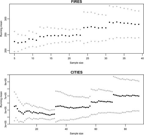
A close examination of the CITIES plot in Figure 3 suggests that the underlying distribution may not have finite variance, as we see large jumps for large sample sizes. This is not surprising, because the tail parameter estimated from the CITIES data is less than 2 (the infinite variance case). The graph for the FIRES data shows more stabilization, which is explained by the tail parameter being larger than 2, suggesting a finite variance. It follows that using the sample mean as the best predictor for future populations of U.S. cities may not work well, and may seriously underestimate the populations. On the other hand, using the sample mean to predict future acreage burnt per fire should work reasonably well, if the sample is large enough.

In summary, we provide two examples of current data that show heavy tail behavior and discuss the common issues when estimating large quantiles that arise when modeling a heavy tailed data with a thin tailed model. We also provide practical reasons for introducing students to heavy tailed data. We believe that the exposure to heavy tailed data and methods is necessary and beneficial for students, as it boosts their opportunities to work on the current and impactful research regarding extreme events, and thus inform policy making processes on issues such as the adaptation to climate change or availability of water resources.

Where in the course can the material/examples of heavy tailed data be incorporated? One place is right after covering the LLN or moments, or when discussing standard distributions and their properties. Another place is after covering the Central Limit Theorem (CLT), where instructors may want to discuss what happens if the finite variance assumption is not satisfied (see the last bullet below).

What questions may be interesting to ask students when analyzing heavy tail data? Here are some examples to consider.

• Why is the mean larger than the 75th percentile for the CITIES data?

• Produce the running mean plot for CITIES (or Pareto or GPD for different α’s) and ask students if it can be inferred from the graphs whether the LLN is satisfied by the distribution generating the data. Follow up with questions about the consequences of such inference when making predictions.

• Explore the impact of changing α on the samples from the Pareto or GPD.

• Fit a light tail standard model (e.g., exponential) to Pareto or GPDs with α’s equal to 0.5, 1, 1.5, and 2, estimate the quantiles and compare with the theoretical Pareto or GPD and/or data quantiles. Discuss the practical consequences of underestimating the high quantiles in applications. Many interesting applications are provided in the literature section of this article.

• Ask students to fit a standard model (e.g., exponential or lognormal, both of which are used in risk analysis) to a sample from a power law tailed distribution and estimate a large percentile as well as a tail probability. What is the problem when using a distribution with a relatively thin tail to model data with a heavier tail? What are the practical consequences of this issue?

• After having students show mathematically that variance does not exist for $\alpha <2$, instructors may ask them to think about the methods and the results that do not work for such distributions, and the consequences for such data analysis and prediction.

• One consequence worthy of mentioning is that the standard form of the CLT, which assumes finite variance of the population, may not work. Thus, many of the inferential methods based on the CLT may not work well for heavy tailed data with infinite variance.

Supplementary Materials

In the Appendix, we provide some resources for the instructors interested in sharing heavy tailed models with their students. They include: (1) representations of the Pareto and Generalized Pareto Distributions (GPD) which are useful for the simulation of heavy tailed data, (2) examples of further reading on the heavy tail distributions, and (3) R code for the graphs used in this paper. In addition, we provide R code for simulating samples from the Pareto and Generalized Pareto Distributions (GPD) and additional references.

Aknowledgments

The authors extend their thanks to the Reviewers, Editors, and Ms. Danelle Clarke for their comments and suggestions that greatly improved this manuscript.

Notes

1 Data from https://www.ncdc.noaa.gov/societal-impacts/wildfires/month/0.csv

2 Data from https://www2.census.gov/programs-surveys/popest/tables/2010-2019/cities/totals/

References

- Cooke, R. M., Nieboer, D. Misiewicz, J. (2014), Fat-tailed Distributions: Data, Diagnostics and Dependence, Hoboken, NJ: Wiley.
- Clauset, A., Shalizi, C. R., and Newman, M. E. J. (2009), “Power-Law Distributions in Empirical Data,” SIAM Review, 51, 661–703. DOI: 10.1137/070710111.
- Gabaix, X. (2009), “Power Laws in Economics and Finance,” Annual Review of Economics, 1, 255–293. DOI: 10.1146/annurev.economics.050708.142940.
- Girvan, M., and Newman, M. E. J. (2002), “Community Structure in Social and Biological Networks,” Proceedings of the National Academy of Sciences, 99, 7821–7826. DOI: 10.1073/pnas.122653799.
- Greiner, M., Jobmann, M., and Lipsky, L. (1999), “The Importance of Power-Tail Distributions for Modeling Queueing Systems,” Operations Research, 47, 313–326. DOI: 10.1287/opre.47.2.313.
- Gustar, A. (2020), “The Laws of Musical Fame and Obscurity,” Significance, 17, 14–17. DOI: 10.1111/1740-9713.01443.
- Jeske, D. R., and Chakravartty, A. (2006), “Effectiveness of Bootstrap Bias Correction in the Context of Clock Offset Estimators,” Technometrics, 48, 530–538. DOI: 10.1198/004017006000000110.
- Malevergne, Y., Saichev, A., and Sornette, D. (2013), “Zipf’s Law and Maximum Sustainable Growth,” Journal of Economic Dynamics and Control, 37, 1195–1212. DOI: 10.1016/j.jedc.2013.02.004.
- Navidi, W. (2007), Statistics for Engineers and Scientists, (5th ed.), New York: McGraw Hill.
- Newman, M. E. J. (2005), “Power Laws, Pareto Distributions and Zipf’s Law,” Contemporary Physics, 46, 323–351. DOI: 10.1080/00107510500052444.
- Reed, W., and Hughes, B. (2002), “From Gene Families and Genera to Incomes and Internet File Sizes: Why Power Laws are so Common in Nature,” Physical Review E, 66, 067103(4). DOI: 10.1103/PhysRevE.66.067103.
- Schluter, C., and Trede, M. (2018), “Size Distributions Reconsidered,” Econometric Reviews, 38, 1–16.
- Sornette, D. (2003), Why Stock Markets Crash (Critical Events in Complex Financial Systems), Princeton, NJ: Princeton University Press.
- Sornette, D. (2004), Critical Phenomena in Natural Sciences: Chaos, Fractals, Selforganization and Disorder: Concepts and Tools (2nd ed.), Berlin: Springer.