Using Grayscale Photos to Introduce High School Statistics Teachers to Reasoning with Digital Image Data

Abstract

Statistics teaching at the high school level needs modernizing to include digital sources of data that students interact with every day. Algorithmic modeling approaches are recommended, as they can support the teaching of data science and computational thinking. Research is needed about the design of tasks that support high school statistics teachers to learn new statistical and computational approaches such as digital image analysis and classification models. Using our design framework, the construction of a task is described that introduces classification modeling using grayscale digital images. The task was implemented within a teaching experiment involving six high school statistics teachers. Our findings from this exploratory study indicated that the task design seemed to support statistical and computational thinking practices related to classification modeling and digital image data.

Keywords:

• Algorithmic modeling
• Computational thinking
• Data science education
• Image data
• Statistical thinking
• Task design

1 Introduction

The high school statistics curriculum needs modernizing and expanding to include more of the data that students encounter in their everyday lives (e.g., Gould 2010; Finzer 2013; Ridgway 2016). As students upload and share images through social media platforms and other digital communications, the use of digital images provides a relevant data context for teaching statistics. The analysis of digital image data can support understanding that data are numbers with context (Cobb and Moore 1997) and can encourage students to integrate statistical and contextual knowledge, an essential aspect of statistical thinking (Wild and Pfannkuch 1999). Furthermore, the digital technology context provides an opportunity to co-develop students’ statistical and computational thinking, which aligns with the digital technology goals of New Zealand schools and recommendations for teaching data science (e.g., De Veaux et al. 2017; Gould 2021).

The opportunities for students to integrate statistical and computational thinking with digital image data can be broadened when introduced alongside new approaches to statistical modeling, such as the use of algorithmic models. Algorithmic models have been proposed as conceptually more accessible for students (e.g., Gould 2017) and research with high school statistics teachers suggests teachers with minimal knowledge of algorithmic models are able to quickly develop and interpret formal classification models (Zieffler et al. 2021). To teach algorithmic modeling such as classification with digital images at the high school level, statistics teachers will need access to tools and learning tasks for analyzing digital image data. As part of a larger research study, we created a design framework to inform the development of new tasks to introduce code-driven tools for teaching statistical modeling (Fergusson and Pfannkuch 2021). In this article, we explore the design and implementation of a task for introducing statistics teachers to informal classification modeling with digital images and discuss how the design of the task may have supported the statistical and computational thinking practices observed in the reasoning and actions of the teachers.

2 Teaching Classification Modelling with Digital Images

Images such as photographs provide an engaging and accessible modern data-context for teaching statistics, especially those shared on social media platforms such as Twitter (now X) or Instagram (e.g., Fergusson and Bolton 2018; Boehm and Hanlon 2021). Students can develop variables based on visual features of the photographs, by counting objects visible within the photograph or by sorting the photographs based on a specific quality (e.g., Bargagliotti et al. 2020, pp. 31–35; Fergusson and Wild 2021). These kinds of activities begin to expand students’ notions of data and provide encouragement to see opportunities for data creation everywhere. However, the analysis of digital image data involves more than just an awareness of data and the curiosity to learn from data. To learn from digital image data requires thinking that extends beyond integrating contextual and statistical knowledge (Wild and Pfannkuch 1999) to include the computational (Gould 2021). Lee et al. (2011) proposed that computational thinking requires abstraction, automation, and analysis.

Teaching computational image analysis can involve understanding digital representations of images that are different from the multivariate rectangular datasets commonly used in statistics classrooms. High school statistics students are familiar with datasets where each row represents a different case or entity, and each column represents a different variable or attribute about that entity. Digital image data from a grayscale photo can be represented in this structure, where each row represents a pixel from the image. However, this data structure for a digital image may remove information about the spatial correlation between pixel values. Additionally, using formal mathematics representations, notation, and formulas to introduce image analysis (see Li 2018) could be a potential barrier for engaging a wide range of students. Therefore, when introducing the mathematics of digital image data structures, care needs to be taken to design learning tasks that highlight and promote key statistical concepts (Bargagliotti and Groth 2016). For example, in the Nanoroughness Task discussed by Hjalmarson, Moore, and delMas (2017), students did not directly engage with the mathematical structure of the digital image data for grayscale photos. Instead, students were given physical grayscale photos where the levels of darkness (grayscale numeric values) were represented using a scale legend.

Opportunities to promote statistical reasoning without mathematical representations also exist when manipulating images, such as changing the contrast of a grayscale photograph using histogram equalization. Exploring the distribution of grayscale values lends itself to reasoning with data distributions, where the data are the pixels of the digital image. Existing research about how students reason with distributions (e.g., Bakker and Gravemeijer 2004) can inform task design, in particular reasoning about shape (e.g., Arnold and Pfannkuch 2016), the role of context in interpreting distributional features, and students’ difficulties with interpreting histograms (e.g., Kaplan et al. 2014).

It is also important to use digital image data within learning contexts that are genuine, and where the context is crucial to the design of the learning task (e.g., Weiland 2017). Digital photographs are very commonly used to develop models that predict categorical or numeric outcomes, for example, predicting age from a photograph, or classifying a photo as having either high or low esthetic value (e.g., Datta et al. 2006). Classification models have been included in high school data science or modernized statistics curriculum documents such as the International Data Science in Schools Project (IDSSP, idssp.org/pages/framework.html), Introduction to Data Science (IDS, idsucla.org), ProCivicStat (iase-web.org/islp/pcs) and ProDaBi (prodabi.de). Not only does the use of classification models with digital images provide a genuine learning context, but classification problems may be easier for students to understand than regression problems (Gould 2017).

Algorithmic models such as classification models (e.g., decision trees), however, are not developed in the same way as probabilistic models. Research involving high school statistics teachers indicates the need to consider the role of context and understanding of the use of training and validation phases (Zieffler et al. 2021). Teachers also need to be aware of the different sources of uncertainty in the modeling process, such as objective versus subjective uncertainty (Yang, Liu, and Xie 2019), and how these uncertainties might be articulated by students when completing learning tasks (Gafny and Ben-Zvi 2021). Another consideration is for students to understand that algorithmic models are fallible just like human decision-making is, and therefore teaching and learning needs to account for the human dimension of data work (Lee, Wilkerson, and Lanouette 2021).

There is also the question of what tools to use to teach classification models. We have proposed classifying tools for statistical modeling based on whether they are unplugged, GUI-driven or code-driven (Fergusson and Pfannkuch 2021). We describe code-driven tools as computational tools which users interact with predominantly by entering and executing text commands (code) and GUI-driven tools as computational tools which users interact with predominantly by pointing, clicking, or gesturing. It is a common approach within statistics education to use unplugged tools before moving to GUI-driven tools. Pedagogical approaches include using data cards to create visual representations (e.g., Arnold et al. 2011; Arnold 2019) or shuffling cards by hand to simulate random allocation of treatments to units (e.g., Budgett et al. 2013). Teaching materials from IDS, ProCivicStat and ProDaBi include unplugged modeling with data cards before moving to the computer to develop classification models (e.g., Podworny et al. 2021). Specifically, ProCivicStat uses the GUI-driven tool CODAP (Engel, Erickson, and Martignon 2019), whereas IDS uses a code-driven tool employing the programming language R (R Core Team 2020).

Although code-driven tools can assist the analysis of digital image data, little is known about how high school statistics teachers will balance learning new statistical and computational knowledge within the same task. Emerging research indicates that students may frame problems as either statistical or computational when encountering issues with executing code (Thoma, Deitrick, and Wilkerson 2018) and that building on familiar statistical ideas and matching to modeling actions may support teachers’ introduction to code-driven tools (Fergusson and Pfannkuch 2021). There may also be benefits to using code with respect to a lowering of the cognitive load of the statistical modeling task (e.g., Son et al. 2021), perhaps as code can be used to articulate modeling steps (e.g., Kaplan 2007; Wickham 2018). There is a lack of research involving high school statistics teachers’ reasoning with digital image data, and none that we are aware of that involves them using digital image data to develop classification models.

2.1 Research Question

The purpose of this article is to show how high school statistics teachers can be supported to use statistical and computational thinking practices within the context of informal classification modeling and digital image data. Within this research context, the teachers are positioned as the learners. The research question is: In what ways does the design of the task support statistics teachers’ observable statistical and computational thinking practices when they are exposed to a new learning environment which includes digital image data and classification modeling?

3 Research Approach

As statistical modeling approaches using digital image data and classification algorithms are not currently assessed by the national assessment system in New Zealand, a design-based research approach (e.g., Bakker and van Eerde 2015) was used for the larger research study this article sits within. Design-based research supports the development of solutions to practical problems grounded in real learning environments alongside new and reusable design principles (Reeves 2007). These design principles are theories that aim to support other designers to create or observe similar outcomes (Van den Akker 1999). The design-based research process used for the larger study involved four iterations of four different statistical modeling tasks, the second iteration of which is described in this article. Similar to the other iterations, the second iteration included: (a) identifying a research problem through the analysis of a practical teaching issue; (b) constructing a new learning task informed by existing and hypothetical design principles and technological innovations; (c) implementing and refining the task through a teaching experiment; (d) reflecting and evaluating to produce new design principles and an enhanced task (Edelson 2002; Reeves 2007; McKenney and Reeves 2018). The four new learning tasks were designed as potential learning activities for high school students. As part of the analysis for each task, design decisions were documented through a narrative (see Hoadley and Campos 2022) that included identifying features that were intentionally included in the task to support and develop statistical and computational thinking as well as essential features that seemed to support learning about statistical modeling. Where relevant, aspects of the design narrative are linked to the research literature from statistics, mathematics, and computer science education. Thus, a design narrative is used in this article to inform other researchers and designers.

3.1 Participants and Teaching Experiment

The participants were six experienced Grade 12 statistics teachers. The teachers had taught at the high school level for an average of 10.5 years (mean $=$ 10.5, min $=$ 7, max $=$ 14). None of the teachers had used any programming languages when teaching Grade 12 statistics students, and only one of the teachers had experience using the statistical programming language R. Permission to conduct the study was granted by the University of Auckland Human Participants Ethics Committee (Reference Number 021024). The teachers were participants in the larger study, which involved four full-day professional development workshops. The teaching experiment, which is the focus of this article, took place during the first day of the workshops. This was the first task that required teachers to use a code-driven tool and took place in the afternoon. In the morning session, teachers explored the popularity of cat and dog photos from the website unsplash.com (see Fergusson and Wild 2021).

3.2 Data Collection and Analysis

Teachers worked in pairs and were given access to one laptop computer to assist with completing the task. Screen-based video and audio recordings of the teacher actions, responses, interactions with the software tools and conversations were made used a browser-based tool Screencastify. Teachers were also asked to “think aloud” as they completed the task (Van Someren, Barnard, and Sandberg 1994). At the end of the task a semi-structured group discussion was used to encourage reflective practice, and to capture teachers’ thoughts on the task’s anticipated effectiveness for teaching students.

To identify observable thinking practices, a task oriented qualitative analysis approach was used (Bakker and van Eerde 2015). The transcripts and screen recordings were reviewed chronologically across each of the three phases, and then across each pair of teachers within the same phases. Annotations were made to the transcripts with conjectures about the nature of the teachers’ thinking and reasoning and what features of tasks appeared to stimulate or support these thinking practices. These annotations led to the identification of salient examples from within each phase that would inform the research question, with examples selected through a process of constant comparison (e.g., Creswell 2012; Bakker and van Eerde 2015). Special attention was paid to episodes of teacher thinking and reasoning involving data, models, modeling, computation, and automation, and the computational steps of the statistical modeling activity.

To characterize observable thinking practices as statistical, computational, or integrated statistical and computational, we considered existing frameworks for statistical thinking (e.g., Wild and Pfannkuch 1999), computational thinking (e.g., Brennan and Resnick 2012), and statistical computing (e.g., Woodard and Lee 2021). Statistical thinking practices were characterized as teachers: referring to the context of the statistical modeling task (classifying grayscale photos) when considering what questions to explore and what data was needed; and identifying relevant features in the data and considering what these mean with respect to the context of the statistical modeling task (classifying grayscale photos). Computational thinking practices were characterized as teachers: describing in words or with code how automation and other computational approaches were used to create a data-related product (the classification model); discussing the differences between how humans and computers make decisions; and evaluating the accuracy or usefulness of the data-related product (the classification model) from a humanistic perspective (see Lee, Wilkerson, and Lanouette 2021). Integrated statistical and computational thinking practices were characterized as teachers connecting statistical and computation thinking practices, for example: considering what computational approaches could be used with the data and how these would help their modeling goals; and discussing what they needed to know or change about the data to inform their computational approaches.

4 Task Construction

The statistical modeling task was constructed to introduce code-driven tools to high school statistics teachers. The task started with immersing teachers in the context and familiar statistical experiences, toward describing computational steps, matching code to steps, adapting code through using and tinkering with code-driven tools, and exploring new models. For full detail and discussion on the task design framework used for the construction of the task see Fergusson (2022).

The statistical modeling approach for the task described in this article involved developing classification models using an informal method. The intent for the task was to provide a positive first exposure to reasoning with digital image data using grayscale photos, rather than provide a comprehensive introduction to classification modeling. The statistics teachers were not introduced to any formal algorithms for developing classification models in the task and instead were expected to reason visually with numeric distributions. Only the idea of a decision rule was introduced, and the task required teachers to use an aggregate measure of a numeric variable to classify cases as one of two levels of a categorical variable. The learning goal for the task was for the teachers to create a decision rule to classify grayscale photos as high contrast or low contrast, based on the distributional features of the digital image data. An example of a decision rule is: If the standard deviation is more than 120, classify the photo as high contrast, otherwise classify the photo as low contrast.

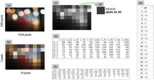
The decision to use digital image data from grayscale photos provided data with different features that can be exploited to support both statistical and computational thinking and was also aligned to the larger research study goal to provide a data science perspective for statistical modeling. The digital image data for the task were thirty popular photos of dogs sourced from the website unsplash.com. Each of these photos was reduced in size and converted to grayscale. Figure 1 shows six different representations of the same photograph that capture the process of converting a color photo to grayscale as well as reducing the dimensions of the image. The different representations illustrate some of the computational steps involved to create a data structure that can be used with classroom statistical software, as well as computational knowledge such as the RGB (red, green, blue) and HEX¹ color systems.

Fig. 1 Six different representations of a photograph: (a) color photo; (b) dimensions reduced; (c) converted to grayscale; (d) HEX code and RGB values; (e) matrix; (f) vector; (g) data frame/table.

Because the teachers had no experience using digital image data or classification models for statistical modeling, two main design decisions were made. The first decision was to use an unplugged approach to introduce classification modeling ideas (see Podworny et al. 2021). The second design decision was to represent the data only using the combined dot and boxplots, on the grounds that teachers were familiar with them through experience with the GUI-driven software tool iNZight (Wild, Elliott, and Sporle 2021).

The teachers were guided through the task by the researcher, the first author, using presentation slides, live demonstrations, verbal instructions, and instructions embedded within interactive documents. The task was designed to take around 90 min to complete. Each of the three task phases is now described through a narrative about further design decisions.

4.1 Phase One: Introduction to Digital Image Data

The first phase of the task immersed teachers within a digital image data context so that they could meaningfully engage with the classification of grayscale photos later. At the start of the phase, teachers were shown a colorful photo of jellybeans, given a brief explanation about digital images and pixels, and shown a color wheel that demonstrated the RGB system for defining the color of each pixel (Figure 2(a)). Teachers were then shown six different colors with their associated RGB values and worked in pairs to discuss answers to four questions that were designed to help teachers learn about the RGB system through noticing patterns (Figure 2(b)).

Fig. 2 Slides used to introduce the RGB color system.

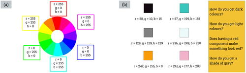
The researcher explained several methods for converting a color photo to grayscale, one of which is to take the average of the RGB values for each pixel and replace the RGB values for that pixel with this one average value (Figure 3(a)).

Fig. 3 Slides used to explain one process for converting a color photo to grayscale.

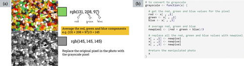
The researcher then demonstrated using the programming language R to convert a digital image from color to grayscale (Figure 3(b)), where the code was specifically written to connect to the visual explanation shown in Figure 3(a). The teachers then watched the researcher use the grayscale function to convert a color photo of a cat to grayscale (Figure 4(a) and (b)) and another function to create a plot based on a random sample of 50 pixels from the grayscale photo (Figure 4(c)).

Fig. 4 The color and grayscale photos used for the demonstration and examples of the four grayscale distributions generated using increasing sample sizes.

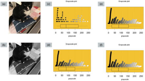
The researcher explained that plot contained a dot plot and a boxplot, and that the shade of gray used for each dot was connected to the grayscale value of that pixel back in the photo. The researcher then demonstrated the different plots created using a random sample of 500 pixels (Figure 4(d)), 5000 pixels (Figure 4(e)) and using all 91,204 pixels (Figure 4(f)). The teachers were asked to discuss how the shape of the distribution changed and how long it took the computer to produce each plot as the sample size increased.

Phase one ended with each pair of teachers being given 10 different grayscale photos and 10 different plots constructed using a random sample of 500 pixels (Figure 5). Each pair of teachers received a unique set of 10 photos. The 10 photos that made up each set were balanced so that each group had a range of light, middle, and dark photos, and contained both high and low contrast photos.

Fig. 5 Ten different grayscale photos and 10 different plots constructed using a random sample of 500 pixels.

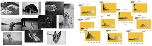
The teachers were asked to connect each photo with its dot plot, with the expectation that they would not be able to accurately connect each photo to its dot plot, a difficult task for photos with similar distributions of grayscale values. The purpose of the connecting activity was to stimulate discussion about the differing features of the sample distributions (see Arnold and Pfannkuch 2016) to lay foundations for reasoning with these distributional features later in the task.

4.2 Phase Two: Introduction to Classification Modelling Ideas

The second phase of the task introduced teachers to classification models and the idea of using an aggregate measure, such as the median grayscale value, to measure the overall “lightness” of a grayscale photo. The task design process for this phase considered how to introduce new knowledge such as decision rules and “training” and “testing” models, alongside more familiar ideas such as measures of central tendency and sampling variation. With respect to the tools used, a decision was made for teachers to use the code-driven tool at the end of the phase, because unplugged approaches were considered more suitable for beginners to build familiarity with the computational steps for classification modeling (see Shoop et al. 2016).

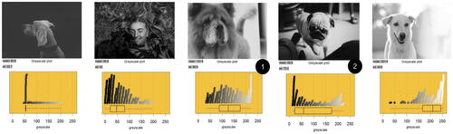
Because the teachers were unfamiliar with classification modeling, familiar statistical ideas related to medians were used to introduce decision rules. Each pair of teachers initially worked with their own set of 10 photos and plots, where each photo was attached to a plot using a sticky dot. The researcher asked the teachers to arrange the photos in order from darkest on the left to lightest on the right, and, after they had ordered the photos, she suggested that perhaps a computational method could be used to sort the photos from darkest to lightest. She asked the teachers to look at the median grayscale value displayed on the boxplot and discuss whether the medians increased in size as the photos changed from dark to light. The direction to teachers to compare their visual judgements of lightness to a statistical measure based on the grayscale distribution was also designed to expose teachers to the difficulties of humans classifying high contrast photos as light or dark. An example of a conjectured “line up” is shown in Figure 6. Note that the median for each distribution of grayscale values (as indicated by the boxplot) generally increases as the overall lightness of the photo increases. However, the photos and plots labeled 1 and 2 break the pattern of increasing medians.

Fig. 6 Example of a conjectured “line up” of photo-plot pairs.

Continuing with the unplugged approach, the teachers were then asked to develop a model to sort the photos into light or dark based on the median grayscale value from a random sample of 500 pixels from the photo. The researcher demonstrated that the computational steps involved reading in an image, taking a random sample of 500 grayscale values, and then deciding if the image was dark or light based on the median of the sample grayscale values being above or below a certain value. Although the classification of photos as dark or light is not binary, the decision was made to use this artificial dichotomization to provide a “stepping stone” for later in the task, when the classification would be based on matching “human” judgments of high or low contrast with computational decisions. The teachers were asked to develop their own decision rule by first sorting the photos into “light” or “dark” visually, and then examining the median grayscale value for each sample distribution. The teachers were then told not to move the photos and decide on a decision rule in the form of a “cut off” value. After the teachers decided on a “cut off” value, they had to count how many of their photos would be correctly classified according to their rule.

The researcher explained that the teachers had just “trained” their model and now they had to test it using new data. The decision to use a different set of dog images for “testing” their model was an important new idea for developing classification models that teachers had not used before. The teachers were instructed to swap their set of 10 photos and plots with another pair of teachers, to apply their classification model to this set of photos, and to count how many of the photos would be correctly classified according to their rule and their sorting of the photos. The teachers were then given back their original set of 10 photos and plots and asked to describe their classification model to the other teachers and how well it worked on the “testing” data. Following this, the teachers were asked to discuss if they thought using the mean grayscale value might be a better way than the median to sort and classify grayscale photos in terms of their lightness.

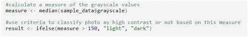
The researcher then demonstrated how to use R code to articulate their model based on their decision rule for the median to classify a particular photo as light or dark. Figure 7(a) shows the code provided and the two lines of code that were the focus of the demonstration, which have been labeled 1 and 2. The line of code labeled 1 needed to be modified by the teachers to match their model, for example, using a different “cut off” number than 200 for the median grayscale. The line of code labeled 2 needed to be adapted by teachers to use the model with different dogs based on the photo number, for example, changing 18 to photo number 21. Figure 7(b) shows the physical photo-plot pairing recreated digitally for dog number 18, with the label “dark” added to the top left-hand corner of the photo, which has been labeled 3.

Fig. 7 Example of a classification model articulated with code with the output generated from the model.

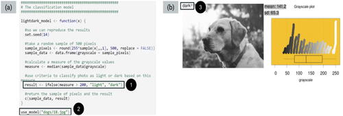
The teachers were then given access to a RMarkdown (Allaire et al. 2021) document that contained the R code shown in Figure 7(a) and were asked to adapt the code to match the classification model they had developed. At this stage of the task the teachers did not know if they had correctly connected their photos to the plots, so when they changed the code based on their photo numbers, they were able to check. The teachers were asked to adapt the provided code but change the classification model to be based on the mean grayscale value.

Rather than supply teachers with a pre-labeled dataset, the decision was made to involve teachers in the labeling, using their subjective judgements of “light” and “dark”. Our reasoning for this task design decision is similar to Podworny et al. (2021). While we understand that this is not a typical context for classification modeling, real applications of classification modeling also rely on subjective judgements made by humans (e.g., Datta et al. 2006). Another purpose of the light or dark classification task was to stimulate discussion about the grayscale distributions of high contrast photos and so motivate a need to develop a model to classify such photos. That is, we expected the teachers to notice that photos that were difficult to classify as light or dark were often ones that were high in contrast.

4.3 Phase Three: Exploration of “High-Contrast” Grayscale Photos

The third phase of the task required teachers to develop their own rule for determining high contrast photos, using features of the sample grayscale distributions. A decision was made to allow time for teachers to develop their classification model using an unplugged approach first, before providing them with a code-driven tool to explore changes to their model.

Teachers were shown a video featuring a photographer discussing high contrast photos (see youtube.com/watch?v = 31qVHQbd0JU), for the dual purpose of explaining what high contrast was and also to reinforce that high contrast grayscale photos are a desirable esthetic. The teachers were then asked to use their 10 photo-plot pairs from the earlier two phases to develop a model to sort the photos into high or low contrast. The researcher encouraged them to look again at their photo-plot pairs, to split them into photos they thought were high contrast versus those they did not and to consider any features of the distributions of grayscale values that could be used to identify photos with high contrast.

After around 5 min of the teachers using only the physical photo-plot pairs to explore their ideas for classifying photos as high contrast, teachers were provided with a RMarkdown document that contained instructions for the rest of the phase and “starter code,” similar to the code shown in Figure 7(a). At the start of the document, teachers were asked to write a couple of sentences describing how they developed their model in response to the following questions: What did you notice about the photo/plot pairs? What feature of the grayscale pixels are you using? What is your criterion for when a photo is high contrast and when it is not?

The teachers were then asked to adapt the code provided to articulate the classification model they had developed. The document also asked teachers to test their model using another random sample of 10 dog photos, with code provided that could be adapted and copied to support them to do this. Teachers were asked at the end of the document to write about what they learned from testing their model in response to the following questions: How well did the model work with another sample? Can you identify any reasons why the model worked better/worse? Do you have any ideas of how to modify your model or approach?

5 Results

Drawing on existing statistical knowledge, all the teachers were able to describe distributional features of digital image data. The teachers used these distributional features to create rules to classify grayscale photos as high contrast or not high contrast. In particular, the teachers attempted to connect different features of distributions, such as skewness or bimodality, to visual features of high contrast photos, using statistical measures such as means, medians and standard deviations. All the teachers successfully modified existing code to engage with digital image data and to articulate their classification model. We now present in more detail the results of the teachers’ interactions with the phases of the task and the observed statistical and computational thinking practices.

5.1 Phase One: Introduction to Digital Image Data

The focus for phase one was integrating new computational knowledge related to digital data with familiar statistical knowledge related to distributions and the teachers spent 42 min working on this phase. After the teachers were introduced to new ideas related to digital images, including converting color photos to grayscale and visualizing random samples of pixels from grayscale photos, they began to reason with digital data during the connecting activity used for this phase. Figure 8(a) shows Amelia and Ingrid’s connected photos and plots.

Fig. 8 Amelia and Ingrid’s connected photos and plots.

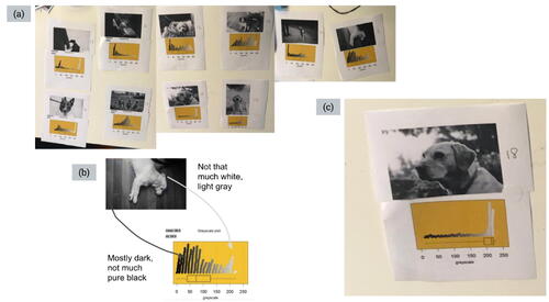
When asked to connect the grayscale photos to the plots of the samples of grayscale values, a visual proportional strategy was used by all pairs of teachers. Using this strategy, the teachers attempted to estimate the proportions of different shades of gray for each photo and then tried to connect these proportions to the dot plot representation of the sample of grayscale values. This was evident through the teachers’ use of descriptions such as “more white” and “a lot of black”. The teachers did not use numeric values for the shades of gray, which could have been read from the axis of the plots. Instead, they used descriptions of shades of gray such as “pure black” and focused on distinctive areas of darker shades of gray and lighter shades of gray (Figure 8(b)).

When describing distributions during the connecting activity, examples of words used included “extreme ends” or “edges” when referring to tails and “high pitched” or “spikes” when referring to modal grayscale values. These words, and the visual proportional strategy, indicated that the teachers were focused on distributional shape. More formal descriptions of distributional features, such as “skewness,” “bi-modality,” or “outliers,” were used toward the end of the connecting activity when teachers compared their photo-plot connections with each other and within a researcher-led group discussion. For instance, the following discussion between three of the teachers was initiated by the researcher asking if they had used the summary statistics printed on the plots to help them make their connections.

Naomi: No, it was the distribution, it was totally about the distribution.

Amelia: We looked at things like bimodal, lots of contrast, or if it was particularly at one end if it was dark or particularly at the other one end if it was light.

Naomi: Also, how far up the scale it was, wasn’t just the shape. Was it pure white, or the grayer shades?

Nathan: We were focusing on dots, focusing on the grayscale of the dots.

Naomi: But, actually, variation was very important, because it wasn’t just the mean it was also, “Is it bimodal?”, as opposed to a normal [shape].

Note in this discussion that from the teachers’ own perspective, distributional shape was the main factor used to make matches. Naomi also referred to “…how far up the scale it was …. was it pure white, or the grayer shades?” and Nathan referred to “…focusing on the grayscale of the dots”, both confirming the use of a visual proportional strategy.

The teachers did struggle, as anticipated, to match some photos using a visual proportional strategy. One contributing factor to their difficulties was that the grayscale plots were based on a random sample of 500 pixels. Toward the end of the connecting activity, after the teachers had walked around the room and looked at the other pairs’ matches, Naomi and Amelia discussed why connecting photos to plots using the visual proportional strategy may have been an issue. The discussion began when Naomi noticed how Amelia and Ingrid had matched photo number 18 to a dot plot (Figure 8(c)).

Naomi: I would not have picked that one …I’m just thinking there isn’t enough white to be down there …it’s a little bit of white but it’s not the biggest.

Amelia: Because it’s just a sample of the pixels, you could have got a sample …so you might not have got as many from here [pointing to an area on the photo] as you would expect.

Naomi: But a sample of 500 should be representative.

Amelia: You’re right, but if you’ve got just an area, like this one where that’s the area where all the white is, if that area wasn’t sampled quite as much as that area [pointing to an area of black], you wouldn’t get the same kind of picture [referring to the dot plot] …but you’re right, 500 is a pretty big sample.

We interpreted that Amelia believed a random sample of 500 pixels may provide insight into the underlying shape of the distribution of grayscale values for all pixels, but that she also was aware that the proportion for each of the possible 256 individual shades of gray could vary considerably between samples. However, Naomi appeared to believe that for any distribution, a sample of 500 should be representative, perhaps not realizing that distributional shape is dependent on both the sample size (500) and the number of values in the sample space (256).

Another strategy used to connect photos with plots was demonstrated by Nathan and Harry, who attempted to order their photos from darkest to lightest using a visual proportional strategy, before connecting the plots to the photos. Amelia and Ingrid stated in the group discussion at the end of this phase that they had seen this strategy being used and tried to use it but, “…. the ones we had left were all the gray ones, it was really hard to put them darkest to lightest, using the mean wouldn’t have even been helpful even if we had used it.” Indeed, the visual proportional strategy appeared to be the most successful for teachers when the visual features of the photos were “strong”, with Amelia commenting that, “where it [the photo] had contrast, you’re looking for bimodal. Where it was really dark or really light, you were looking for skewness.”

The results from phase one indicated that teachers were beginning to think computationally about distributions, because they were able to conceive of shades of gray from a photo as numeric data points. Their use of visual proportional and distributional reasoning to make connections between features of plots and photos showed how they were using their statistical thinking. Connecting grayscale photos with features such as high contrast using human visual judgements was easier for the teachers than connecting photos with less distinctive features, and these judgements were also influenced by reasoning related to sampling variation.

5.2 Phase Two: Introduction to Classification Modelling Ideas

The focus for phase two was introducing new computational ideas associated with classification modeling through drawing on familiar statistical ideas related to medians and means. The teachers spent 32 min working on this phase. When asked to order the photos from dark to light, all pairs of teachers found photos where they struggled to decide their “lightness” position relative to the other photos. Ingrid explained that, “…these [photos] are the hard ones because of the high contrast” and Naomi elaborated, “high contrast makes us think of light …because when we see high contrast, we’ve got a lot of light around.” All pairs of teachers expressed a lack of confidence that they had ordered the photos “correctly” from darkest to lightest.

The researcher asked the teachers to look at the medians of distributions attached to the sorted photos and to examine if the medians increased in size as the photos increased in lightness. The teachers observed that for their set of 10 photos and plots, the medians did not always increase, which led them to perceive that they were at fault and that they had incorrectly ordered the photos from darkest to lightest. This perception was captured in a discussion between some of the teachers and the researcher below, which took place after the teachers had developed their own decision rules for classifying a photo as “dark” or “light” based on the median grayscale value.

Amelia: We struggled to say which was light and which was dark, I don’t know that a human is very good at this.

Naomi: No, that’s right, I would totally agree!

Amelia: If you’re training the computer to do it, you might be training the computer to do it better than you could do it, so you’re not like trying to get it to match the human model, it’s [the computer] doing it better.

Researcher: It depends, your target audience is still how a human perceives lightness or darkness.

Amelia: Yeah, but to excuse the pun, there’s a lot of gray in the middle.

Researcher: Yeah, shades of gray!

Naomi: As humans we’re responding to other things than the median. I noticed that if something was taken in lower light, I would want to classify it as dark rather than just looking at the amount of light and dark because my brain starts thinking, “Oh yes, darker picture, taken in lower light” even if maybe there’s quite a lot of whiteness in it.

Researcher: So, what we’re doing at this stage is we’re just developing an idea. We’re not saying the median is the best way to do it or that it even is possible. It’s this idea of “What if?” Could we try this out, could we try and classify photos using the median?

Note that Naomi and Amelia articulated why human decision making might not be as consistent as the median measure used by a computer. As the classification model needed to reproduce human judgements using the median, the researcher reminded them the model is based on human perception and that the model may not be correct. Some evidence that the teachers were able to incorporate subjective human esthetics as the basis for the classification model was the “cut off” value used for the decision rule. Figure 9 shows the decision rule used by Harry and Nathan, articulated with R code.

Fig. 9 The decision rule used by Harry and Nathan.

The code shows that photos with a sample median grayscale value greater than 150 are classified as “light.” Harry explained that they, “…found the cut off point for the median was higher than the middle of the distribution, as to our eyes it was more natural to put in the median where we did.” The teachers also demonstrated some understanding of difficulties with dichotomizing numeric variables when they tested their classification model on 10 photos from another pair of teachers and identified that photos with median grayscale values “around the boundary” were often misclassified using their decision rule.

Although the focus for this phase was on introducing new computational ideas related to classification modeling, the teachers also continued to reason statistically through thinking about distributions and the impact of sampling variation. This was apparent when the teachers were asked to consider whether the median or the mean would be a better measure for the overall lightness for a grayscale photo. Amelia shared her reasoning in the following excerpt:

The reason we thought the median was better was that where you’ve got pictures with like a big chunk of dark or a big chunk of light, you often have got the skewed distribution, so it would pull the mean one way. But that big chunk of light makes the picture look light, so you actually want to go with the median because you want to go with that big chunk.

The other teachers shared similar reasoning about a preference for using the median as the measure of overall lightness that best matched a human visual judgment. None of the teachers commented on the usefulness of using a measure of central tendency for distributions that were bimodal, however, Nathan indicated that he had begun to consider measures of spread when he agreed with using the median, “…because of the variation that you have here with your lights and darks.” The impact of sampling variation on the performance of the classification model was also discussed by Ingrid, when she observed that the median jumped around more for random samples of 500 pixels than the mean did.

After the teachers had developed their decision rule to classify photos as “dark” or “light” based on the median grayscale, the researcher realized that more information about classification models was needed. In particular, she reminded the teachers that for a classification model, “the goal is not 100% correct” and that they needed to be careful not to overfit their model. This new knowledge was then used by the teachers as part of their evaluation of the classification model for this phase. To illustrate, Harry reminded Nathan that, “…there is no perfect model, 90% will do” and not to focus too much on “getting the model to work” for special cases. Ingrid also specifically discussed being mindful of “overfitting” when describing their model to the other teachers at the end of the phase.

The results from phase two indicated that teachers were beginning to think computationally with regards to how a human decision, such as subjectively measuring the lightness of a grayscale photo, could be automated using a classification model based on statistical properties of data. The teachers also appeared to recognize that classification models are evaluated based on the percentage of correct classifications and that this percentage may not be 100%, suggesting that statistical and computational thinking were being supported. The use of familiar statistical ideas within the context of digital image data seemed to encourage statistical thinking practices involving new applications of the median and mean to summarize a distribution.

5.3 Phase Three: Exploration of “High-Contrast” Grayscale Photos

The focus for phase three was for teachers to integrate statistical and computational ideas as they developed and used models to classify “high contrast” grayscale photos with R code. This phase was less structured than the previous phases and provided an opportunity to observe how the teachers applied the new statistical and computational ideas introduced earlier. To gain an understanding of each pair’s modeling process, it was decided to analyze the transcripts and screen recordings with respect to how much time in minutes each pair of teachers spent developing their model, articulating their model using code, and checking or changing their model. The analysis also considered when the unplugged (physical) photos and plots were used and when the code-driven tool was used. A visual summary of this analysis is shown in Figure 10.

Fig. 10 A visual comparison of the modeling process used by each teacher pair.

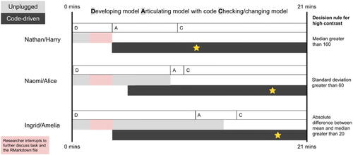
Figure 10 also describes the classification model developed by each pair of teachers, for example, Ingrid and Amelia’s final decision rule for high contrast was an absolute difference between the mean and median greater than 20. The star indicates the time at which the pair of teachers expressed that they were happy with their model. We now use Figure 10 and additional results to compare and describe the modeling processes used by the three pairs of teachers.

The process used by all the teachers to develop a classification model for high contrast grayscale photos involved:

1. making a conjecture about why the photo is high contrast, using human visual analysis/observation

2. making a conjecture about what statistical measure(s) might capture what the human has analyzed/observed, using the sample distribution of grayscale values for that photo

3. formulating a decision rule using a statistical measure from the sample of grayscale values and using this rule with at least one photo to see if it “worked.”

Figure 10 shows each pair of teachers spent differing amounts of time developing their model, ranging from around 2 min for Nathan and Harry to around 11 min for Ingrid and Amelia. The use of the tools provided also differed for each pair of teachers. As Figure 10 illustrates, Nathan and Harry did not use the unplugged tool (physical photos and plots) and the code-driven tool simultaneously while developing their model, in contrast to the other pairs of teachers. Notably, Ingrid and Amelia used both tools simultaneously for around 10 min while developing their model and then articulating their model with code. All pairs of teachers successfully articulated their model using R code, with the amount of time for each teacher pair depending on the complexity of their decision rule and their familiarity with using the code-driven tool. Naomi and Alice spent the longest time checking or changing their model before expressing happiness with their model. When checking or changing their model, the teachers did not always clearly differentiate between using training data or testing data.

We now examine the emergent reasoning of each pair separately as they developed models to classify “high contrast” grayscale photos. After doing a Google search for “high contrast,” Nathan and Harry discussed high contrast in terms of bimodality but then used the same model they developed for classifying “light” photos to classify the physical grayscale photos as “high contrast.” After the researcher interrupted the teachers to discuss how to use the RMarkdown document provided for this phase, Nathan and Harry moved to the computer and only used the code-driven tool for the rest of the phase. They took much longer to articulate their model than the other teachers, struggling at first to figure out how to run the code and consequently visualize the results within a RMarkdown document.

Nathan and Harry were much quicker to accept their model, with Nathan stating, “we accomplished our task!” after testing just one photo. When the researcher asked how many photos they had tested, Nathan replied, “one so far …before we continued, we wanted to make sure it worked.” We interpret Nathan’s reference to making “sure it worked” to be a reference to their code working, in that computationally they were able to make their model work. The computational focus appeared to be confirmed later in the phase when Naomi and Alice shared the model they had developed, which was based on standard deviation, and Nathan said, “we probably should have changed to standard deviation or something …we just went into robot mode!” Standard deviation was a feature Nathan and Harry had discussed with reference to high contrast in phase one, and therefore after being given the model from Naomi and Alice, they were able to adjust their code and use Naomi and Alice’s model to classify a few photos as high or low contrast using the standard deviation.

Naomi and Alice began the phase with a pre-determined idea to use spread as the statistical measure to identify high contrast photos, as they had noticed in phase two that high contrast photos tended to have grayscale distributions with large standard deviations. Naomi stated, “variation is what was important,” and consequently they explored the interquartile range and the standard deviation as measures for the decision rule of their classification model. When they sorted their photos into high and low contrast, they did not always agree on whether an individual photo was high contrast or not. When disagreements arose, these were often resolved by sorting the photos according to their current decision rule and then considering if they still believed that the photo was high contrast or not.

Naomi and Alice used all 10 of their photos to develop their model, and after quickly articulating their model with code, checked their model with “new” photos from outside their training data. The teachers agreed on a decision rule for their classification model that photos with a “standard deviation greater than 60” would be classified as high contrast. Like phase two, when the teachers mentioned the difficulty of dichotomizing numeric variables, Naomi and Alice realized that photos with “standard deviations close to 60” were “borderline” and the most likely to be misclassified.

Ingrid and Amelia demonstrated a more exploratory approach and consequently took longer to develop their model. Figure 11 shows screenshots from the teachers’ RMarkdown-generated HTML document and provides a description of the thinking they used to develop their classification model and the code they modified to articulate their model.

Fig. 11 The classification model developed by Ingrid and Alice.

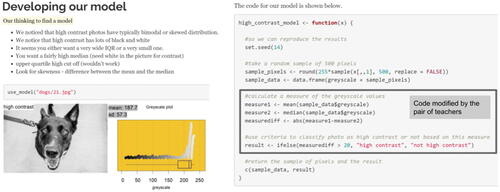
Ingrid and Amelia appeared to be more open to exploring more than one way of classifying high contrast photos and considered bimodality, skewness, and large proportions of “black” and “white” as features of the grayscale distributions that might indicate a high contrast photo. The teachers attempted to translate these distributional features into different decision rules, for example, by noticing high contrast photos have either “a very wide IQR or a small one” or that “you want a fairly high median.” Ingrid and Amelia continued to use the unplugged physical photos and plots alongside the code-driven tool when developing their model. Using both tools appeared to help them quickly repeat the process of making conjectures about high contrast based on human visual analysis of a photo, making conjectures about what statistical measure(s) might capture the human visual analysis, and then formulating and using a decision rule based on a statistical measure to see if the rule worked.

Ingrid and Amelia also considered how their conjectures for statistical measures and decision rules could be expressed using code. For example, after examining the physical plots in front of her, Ingrid remarked, “you could look at the min and the max …I’m thinking about things you could actually put into our model.” Note in Figure 11, the teachers described that they wanted to use a decision rule based on the upper quartile but it “wouldn’t work.” Indeed, Ingrid and Amelia tried to modify the code to create a measure based on the upper quartile, but as this was not a specific function provided by the code-driven tool, they disbanded this attempt. Similarly, Ingrid stated, “it’s kind of hard to find a model that will pick up both skewness and bimodality at the same time,” referring to their knowledge about how to articulate this model computationally with the code provided.

Another reason why the development of their model took longer than the other teachers was that for each idea they had for a decision rule, they would try it out with several photos. If they found one photo that wasn’t correctly classified by the rule, after confirming that they still thought it was high contrast, they would discard the rule. Like Naomi and Alice, they were prepared to change their judgment of whether a photo was high contrast or not, to get their model “to work.” However, toward the end of the development phase of their model, Ingrid suggested that they should forget about one of the photos they were using to develop a model, saying, “maybe it’s just an odd ball.” Although Amelia initially resisted, she then agreed with Ingrid’s justification that they are, “trying to find a model that will work in many cases but not necessarily perfect.” We interpreted this change of approach as an indication that the teachers had begun to evaluate a classification model from the perspective of Does our model get the photos correct most of the time? rather than Can our model cope with the “weird” or “tricky” photos?

The results from phase three indicated that all the teachers were developing and comparing classification models, that is, an integration of statistical and computational thinking practices could be observed. The teachers were creating new measures, a statistical thinking practice, which took different forms of variation into account, and they demonstrated they could articulate their decision rule with code, a computational thinking practice. The last phase of the task was described by Naomi, with agreement from the other teachers, as providing an important learning experience of “trying to take something complex and create a statistical measure for it.”

6 Discussion

The purpose of this article was to show how teachers can be supported to use statistical and computational thinking practices within the context of informal classification modeling and digital image data. We observed that all teachers were able to: (a) connect visual features of grayscale photos with features of sample distributions of grayscale values; (b) create rules to classify grayscale photos in different ways; and (c) use code-driven tools to interact with digital image data and to articulate classification models. These three main observations indicate that the design of the task seemed to support statistical and computational thinking practices. As this was a small-scale exploratory study, the findings from our study cannot be generalized to all statistics high school teachers.

The research question for this article is focused on the ways in which the design of the task supported teachers’ observable statistical and computational thinking practices. The design decisions made when constructing the task seemed to provide a positive “first exposure” to classification modeling with digital image data. We now discuss three specific design decisions that may have assisted teachers’ statistical and computational thinking practices: (a) framing the task in terms of distributions; (b) using a data science unplugged approach; and (c) encouraging human-driven informal model building. As part of the design narrative, we make tentative links between these three specific decisions and the results presented about teachers’ emergent reasoning and actions as well as linking these design decisions to the relevant literature.

6.1 Framing the task in Terms of Distributions

The task directed teachers to reason with distributions throughout the task rather than leaving the analytical approach open to the teachers (see Hjalmarson, Moore, and delMas 2017). We believe this decision provided a way for the teachers to “look” at the digital image data through a familiar lens (see Wild 2006) and supported the introduction of new computational knowledge by extending the familiar into unfamiliar data science approaches (Biehler and Schulte 2017). A key task design feature appeared to be the connecting activity, where teachers physically connected photos (representations of the population distributions of grayscale values) with dot plots (representations of sample distributions of grayscale values), that is, connecting computational and statistical thinking practices. The activity stimulated teacher discussion about distributional shape (see Arnold and Pfannkuch 2016) and helped to support the teachers to successfully reason with digital image data through initially considering the pixels as the cases belonging to each photo. Once the teachers were able to connect the sample distributions of grayscale values with the grayscale photos, the connected photo-plots became the cases that could be summarized using a measure such as the median. The approach to draw teachers’ attention to specific features of a distribution, in our case the median grayscale of the distribution and the lightness of the connected grayscale photo, is consistent with the findings of Arnold et al. (2011).

6.2 Using a Data Science Unplugged Approach

The decision to focus on distributions for this task was strongly linked to the decision to use a data science unplugged approach. The use of physical grayscale photos and dot plots of sample grayscale distributions seemed to assist in analyzing digital image data and reduced the focus on mathematical structures. The physical sorting of the connected photo-plots into different groups for classification (e.g., light vs. dark) appeared to offer similar benefits to the “hands-on” activities used within learning progressions for simulation-based inference with respect to modeling ideas (e.g., Chance, delMas, and Garfield 2004; Zhang, Tucker, and Stigler 2021). We also observed that some teachers continued to refer to physical stimuli even when they had access to the code-driven tool, similar to what was found with another task (Fergusson and Pfannkuch 2021).

The data science unplugged approach used for the task is also consistent with the pedagogy described by Shoop et al. (2016) with respect to teaching robotics, where students work together to build models for computational solutions and present these models to the class for discussion before developing code. In our results we observed that teachers’ statistical and computational thinking practices seemed to be supported as they were able to learn new ideas related to classification models and describe the computational steps in their own words, before articulating their model using readable code (Wickham 2018), an observable example of computational thinking practice. The readable code was made possible through functions that were named to match physical and described actions. However, a limitation of the data science unplugged approach is that the teachers’ experiences with evaluating classification models were small scale. The training and testing datasets only contained 10 photos each and the hands-on approach prevented “scaling up” the evaluation of their classification models. Similar to the teachers observed by Zieffler et al. (2021), the approach did promote some initial modeling approaches that were based on overfitting specific features of grayscale photos. As a “first exposure” learning task, the task seemed to provide a foundation for further development of classification modeling ideas.

6.3 Encouraging human-Driven Informal Model Building

The design decisions to frame the task in terms of distributions and to use a data science unplugged approach were connected to the decision to encourage human-driven model building. Heeding the same call as Lee, Wilkerson, and Lanouette (2021) to take a humanistic stance toward data science education at the school level, the task provided students with personal and direct experiences with data and measurement. Notably, the sample distributions of grayscale values were provided for the teachers, and no pre-labeled datasets were made available, as is commonly the case with introductory classification modeling activities (e.g., Engel, Erickson, and Martignon 2019; Zieffler et al. 2021). Similar to the task developed by Horton, Chao, and Finzer (2023) to explore how students produce data from text to classify clickbait, the teachers needed to connect features they perceived as humans (e.g., high contrast grayscale photos) to features of the data (e.g., skewness of distributions) to computer extractable features (e.g., calculating the difference between the mean and median for a random sample of grayscale pixels), before they could develop rules that could be used to classify photos (Figure 11), an observable example of an integrated statistical and computational thinking practice. These human-driven decisions led to uncertainty with the modeling process, particularly as the teachers often doubted their own ability to classify photos as light or dark, or as high or low contrast. In our results, we presented examples of the teachers grappling with the differences between how humans and computers make decisions. We contend that by not providing a complete and accurate dataset and relying on human choices for both the measures and decision rules, the different sources of uncertainty that are faced by data analysts (see Yang, Liu, and Xie 2019) were effectively incorporated into the learning task.

Even though formal classification models were not introduced, we note that when Datta et al. (2006) attempted to create classification models for esthetics of photographs using formal computational approaches, they discussed similar difficulties that our teachers discovered, specifically issues with dichotomizing numeric variables. A teaching challenge is how to combine thinking like a computer and thinking like a human (see Biehler and Fleischer 2021). On the one hand, statistical thinking requires learners to understand that data are numbers with context (Cobb and Moore 1997) and thus humanistic perspectives of model outputs are needed that account for contextual implications. On the other hand, we found that the context did at times distract the teachers from forming more general ideas about statistical models (see Pfannkuch 2011; Biehler and Fleischer 2021; Zieffler et al. 2021). Similar to Hjalmarson, Moore, and delMas (2017), we found that not all teachers developed a statistical measure that incorporated the variation of grayscale pixels within a photo, a statistical thinking practice. Overall, more research is needed on how and whether human decisions should be encouraged as part of learning about modeling approaches.

6.4 Implications for teaching and Research

The outcomes of this study have several implications for teaching and future research. Similar versions of the statistical modeling task used in this study have been implemented at non-research workshops with high school statistics teachers and students, and with introductory level statistics students. These informal implementations of the task indicate that similar thinking practices could be observed when using the task with students. Hence, researchers and teachers could consider in what ways the task design components encouraged different observable thinking practices and incorporate similar task design features when developing and implementing their own tasks. Further research is planned to collect and analyze student responses to the task and use these to refine our characterizations of observable integrated statistical and computational thinking practices. Research is also needed to explore how the participation of statistics teachers in professional development workshops like those used in our study impacts their teaching practice.

7 Conclusion

We have proposed some practical design solutions for balancing the learning of new statistical and computational ideas when introducing code-driven tools for statistical modeling. Using an unplugged data science approach, the task provided an accessible introduction for the teachers to use digital image data to develop classification models using an informal method. An embedded approach of drawing on familiar statistics ideas first before extending these ideas into less familiar territory appeared to support statistical and computational thinking practices related to classification modeling.

Acknowledgments

We thank the reviewers for their very helpful comments and suggestions on how to improve this article.

Data Availability Statement

The authors confirm that the data supporting the findings of this study are available within the article.

Disclosure Statement

No potential conflict of interest was reported by the author(s).

Notes

1 Hexadecimal: A six-digit combination of numbers and letters defined by its mix of RGB.

References

- Allaire, J., Xie, Y., McPherson, J., Luraschi, J., Ushey, K., Atkins, A., Wickham, H., Cheng, J., Chang, W., and Iannone, R. (2021), “Rmarkdown: Dynamic Documents for R,” RStudio. Available at https://rmarkdown.rstudio.com
- Arnold, P. (2019), “What Pets Do the Kids in Our Class Have?” Statistics and Data Science Educator. Available at https://sdse.online/lessons/SDSE19-003
- Arnold, P., and Pfannkuch, M. (2016), “The Language of Shape,” in The Teaching and Learning of Statistics, eds. D. Ben-Zvi, and K. Makar, pp. 51–61. Cham: Springer. DOI: 10.1007/978-3-319-23470-0_5.
- Arnold, P., Pfannkuch, M., Wild, C. J., Regan, M., and Budgett, S. (2011), “Enhancing Students’ Inferential Reasoning: From Hands-On to “Movies,” Journal of Statistics Education, 19. DOI: 10.1080/10691898.2011.11889609.
- Bakker, A., and Gravemeijer, K. (2004), “Learning to Reason about Distribution,” in The Challenge of Developing Statistical Literacy, Reasoning, and Thinking, eds. D. Ben-Zvi and J. Garfield, pp. 147–168. Dordrecht: Kluwer. DOI: 10.1007/1-4020-2278-6_7.
- Bakker, A., and van Eerde, D. (2015), “An Introduction to Design-Based Research with an Example from Statistics Education,” in Approaches to Qualitative Research in Mathematics Education, eds. A. Bikner-Ahsbahs, C. Knipping, and N. Presmeg, pp. 429–466, Dordrecht: Springer. DOI: 10.1007/978-94-017-9181-6_16.
- Bargagliotti, A., and Groth, R. (2016), “When Mathematics and Statistics Collide in Assessment Tasks,” Teaching Statistics, 38, 50–55. DOI: 10.1111/test.12096.
- Bargagliotti, A., Franklin, C., Arnold, P., Gould, R., Johnson, S., Perez, L., and Spangler, D. (2020), “Pre-K-12 Guidelines for Assessment and Instruction in Statistics Education (GAISE) Report II,” American Statistical Association. Available at https://www.amstat.org/asa/files/pdfs/GAISE/GAISEIIPreK-12_Full.pdf
- Biehler, R., and Fleischer, Y. (2021), “Introducing Students to Machine Learning with Decision Trees Using CODAP and Jupyter Notebooks,” Teaching Statistics, 43, S133–S142. DOI: 10.1111/test.12279.
- Biehler, R., and Schulte, C. (2017), “Perspectives for an Interdisciplinary Data Science Curriculum at German Secondary Schools,” in Paderborn Symposium on Data Science Education at School Level 2017: The Collected Extended Abstracts, eds. R. Biehler, L. Budde, D. Frischemeier, B. Heinemann, S. Podworny, C. Schulte, and T. Wassong, pp. 2–14. Universitätsbibliothek Paderborn. Available at https://fddm.uni-paderborn.de/fileadmin-eim/mathematik/Didaktik_der_Mathematik/BiehlerRolf/Publikationen/Biehler_SchultePaderbornSymposiumDataScience20.pdf
- Boehm, F. J., and Hanlon, B. M. (2021), “What is Happening on Twitter? A Framework for Student Research Projects with Tweets,” Journal of Statistics and Data Science Education, 29, S95–S102. DOI: 10.1080/10691898.2020.1848486.
- Brennan, K., and Resnick, M. (2012), April 2012). “New Frameworks for Studying and Assessing the Development of Computational Thinking,” in Proceedings of the 2012 annual meeting of the American Educational Research Association (Vol. 1), April 2012, Vancouver, Canada. AERA. Available at https://web.media.mit.edu/_kbrennan/files/Brennan_Resnick_AERA2012_CT.pdf
- Budgett, S., Pfannkuch, M., Regan, M., and Wild, C. J. (2013), “Dynamic Visualizations and the Randomization Test,” Technology Innovations in Statistics Education, 7. DOI: 10.5070/T572013889.
- Chance, B., delMas, R., and Garfield, J. (2004), “Reasoning about Sampling Distributions,” in The Challenge of Developing Statistical Literacy, Reasoning and Thinking, eds. D. Ben-Zvi and J. B. Garfield, pp. 295–323, Dordrecht: Springer. DOI: 10.1007/1-4020-2278-6.
- Cobb, G. W., and Moore, D. S. (1997), “Mathematics, Statistics, and Teaching,” The American Mathematical Monthly, 104, 801–823. DOI: 10.1080/00029890.1997.11990723.
- Creswell, J. W. (2012), Educational Research: Planning, Conducting, and Evaluating Quantitative and Qualitative Research (4th ed.), Harlow: Pearson.
- Datta, R., Joshi, D., Li, J., and Wang, J. Z. (2006), “Studying Aesthetics in Photographic Images Using a Computational Approach,” in European Conference on Computer Vision, eds. A. Leonardis, H. Bischof, and A. Pinz, pp. 288–301, Berlin: Springer. DOI: 10.1007/11744078_23.
- De Veaux, R. D., Agarwal, M., Averett, M., Baumer, B. S., Bray, A., Bressoud, T. C., Bryant, L., Cheng, L. Z., Francis, A., Gould, R., Kim, A. Y., Kretchmar, M., Lu, Q., Moskol, A., Nolan, D., Pelayo, R., Raleigh, S., Sethi, R. J., Sondjaja, M., Tiruviluamala, N., Uhlig, P. X., Washington, T. M., Wesley, C. L., White, D., and Ye, P. (2017), “Curriculum Guidelines for Undergraduate Programs in Data Science,” Annual Review of Statistics and Its Application, 4, 15–30. DOI: 10.1146/annurev-statistics-060116-053930.
- Edelson, D. C. (2002), “Design Research: What We Learn When We Engage in Design,” Journal of the Learning Sciences, 11, 105–121. DOI: 10.1207/S15327809JLS1101_4.
- Engel, J., Erickson, T., and Martignon, L. (2019), “Teaching about Decision Trees for Classification Problems,” in Decision Making Based on Data. Proceedings of the Satellite Conference of the International Association for Statistical Education (IASE), Kuala Lumpur, Malaysia, ed. S. Budgett, IASE. Available at https://iase-web.org/documents/papers/sat2019/IASE2019/%20Satellite/%20132_ENGEL.pdf?1569666567
- Fergusson, A. (2022), “Towards an Integration of Statistical and Computational Thinking: Development of a Task Design Framework for Introducing Code-Driven Tools through Statistical Modelling,” PhD Thesis, University of Auckland. Available at https://hdl.handle.net/2292/64664
- Fergusson, A., and Bolton, E. L. (2018), “Exploring Modern Data in a Large Introductory Statistics Course,” in Looking Back, Looking Forward. Proceedings of the Tenth International Conference on Teaching Statistics (ICOTS10, July 2018), Kyoto, Japan, eds. M. A. Sorto, L. White, and L. Guyot. International Statistical Institute. Available at https://iase-web.org/icots/10/proceedings/pdfs/ICOTS10_3C1.pdf?1532045286
- Fergusson, A., and Pfannkuch, M. (2021), “Introducing Teachers Who Use GUI-Driven Tools for the Randomization Test to Code-Driven Tools,” Mathematical Thinking and Learning, 24, 336–356. DOI: 10.1080/10986065.2021.1922856.
- Fergusson, A., and Wild, C. J. (2021), “On Traversing the Data Landscape: Introducing APIs to Data-Science Students,” Teaching Statistics, 43, S71–S83. DOI: 10.1111/test.12266.
- Finzer, W. (2013), “The Data Science Education Dilemma,” Technology Innovations in Statistics Education, 7. DOI: 10.5070/T572013891.
- Gafny, R., and Ben-Zvi, D. (2021), “Middle School Students’ Articulations of Uncertainty in Non-Traditional Big Data IMA Learning Environments,” in Proceedings from the 12th International Collaboration for Research on Statistical Reasoning, Thinking and Literacy, Virtual, pp. 40–43, SRTL.
- Gould, R. (2010), “Statistics and the Modern Student,” International Statistical Review, 78, 297–315. DOI: 10.1111/j.1751-5823.2010.00117.x.
- Gould, R. (2017), “Data Literacy is Statistical Literacy,” Statistics Education Research Journal, 16, 22–25. DOI: 10.52041/serj.v16i1.209.
- Gould, R. (2021), “Toward Data-Scientific Thinking,” Teaching Statistics, 43, S11–S22. DOI: 10.1111/test.12267.
- Hjalmarson, M. A., Moore, T. J., and delMas, R. (2011), “Statistical Analysis When the Data is an Image: Eliciting Student Thinking about Sampling and Variability,” Statistics Education Research Journal, 10, 15–34. DOI: 10.52041/serj.v10i1.353.
- Hoadley, C., and Campos, F. C. (2022), “Design-Based Research: What it is and Why it Matters to Studying Online Learning,” Educational Psychologist, 57, 207–220. DOI: 10.1080/00461520.2022.2079128.
- Horton, N. J., Chao, J., Palmer, P., and Finzer, W. (2023). “How Learners Produce Data from Text in Classifying Clickbait,” Teaching Statistics. DOI: 10.1111/test.12339.
- Kaplan, D. (2007), “Computing and Introductory Statistics,” Technology Innovations in Statistics Education, 1. DOI: 10.5070/T511000030.
- Kaplan, J. J., Gabrosek, J. G., Curtiss, P., and Malone, C. (2014), “Investigating Student Understanding of Histograms,” Journal of Statistics Education, 22, 1–30. DOI: 10.1080/10691898.2014.11889701.
- Lee, I., Martin, F., Denner, J., Coulter, B., Allan, W., Erickson, J., Malyn-Smith, J., and Werner, L. (2011), “Computational Thinking for Youth in Practice,” ACM Inroads, 2, 32–37. DOI: 10.1145/1929887.1929902.
- Lee, V. R., Wilkerson, M. H., and Lanouette, K. (2021), “A Call for a Humanistic Stance toward K–12 Data Science Education,” Educational Researcher, 50, 664–672. DOI: 10.3102/0013189X211048810.
- Li, J. (2018), “Statistical Methods for Image Analysis,” available at http://personal.psu.edu/jol2/Li_lecture_highschool.pdf
- McKenney, S., and Reeves, T. C. (2018), Conducting Educational Design Research, London: Routledge. DOI: 10.4324/9781315105642.
- Pfannkuch, M. (2011), “The Role of Context in Developing Informal Statistical Inferential Reasoning: A Classroom Study,” Mathematical Thinking and Learning, 13, 27–46. DOI: 10.1080/10986065.2011.538302.
- Podworny, S., Fleischer, Y., Hüsing, S., Biehler, R., Frischemeier, D., Höper, L., and Schulte, C. (2021), “Using Data Cards for Teaching Data Based Decision Trees in Middle School,” in Koli Calling ’21: 21st Koli Calling International Conference on Computing Education Research, Joensuu, Finland, November 18–21, 2021, eds. O. Seppälä and A. Petersen, pp. 1–3. ACM. DOI: 10.1145/3488042.3489966.
- R Core Team. (2020), R: A Language and Environment For Statistical Computing. Available at https://www.R-project.org/
- Reeves, T. C. (2007), “Design-Based Research from a Technology Perspective,” in Educational Design Research, eds. J. Van den Akker, K. Gravemeijer, S. McKenney and N. Nieveen, pp. 52–56, New York: Routledge.
- Ridgway, J. (2016), “Implications of the Data Revolution for Statistics Education,” International Statistical Review, 84, 528–549. DOI: 10.1111/insr.12110.
- Shoop, R., Flot, J., Higashi, R., Witherspoon, E., and McKenna, J. (2016), “Using Model Eliciting Activities to Engage Students in Computational Thinking Practices in Robotics Classrooms.” in Paper presented at the High Impact Technology Exchange Conference (2016 HI-TECH, July 2016), Pittsburgh, Pennsylvania. Available at https://www.cmu.edu/roboticsacademy/PDFs/Research/CCRC-MEAs.pdf
- Son, J. Y., Blake, A. B., Fries, L., and Stigler, J. W. (2021), “Modeling First: Applying Learning Science to the Teaching of Introductory Statistics,” Journal of Statistics and Data Science Education, 29, 4–21. DOI: 10.1080/10691898.2020.1844106.
- Thoma, S., Deitrick, E., and Wilkerson, M. (2018), “It Didn’t Really Go Very Well”: Epistemological Framing and the Complexity of Interdisciplinary Computing Activities,” in Rethinking Learning in Digital Age: Making the Learning Sciences Count. Proceedings of the 13th International Conference of the Learning Sciences (ICLS) 2018, London, UK (Vol. 2), eds. J. Kay and R. Luckin, pp. 1121–1124. International Society of the Learning Sciences. Available at https://repository.isls.org/bitstream/1/574/1/249.pdf
- Van den Akker, J. (1999), “Principles and Methods of Development Research,” in Design Approaches and Tools in Education and Training, eds. J. Van den Akker, R. M. Branch, K. Gustafson, N. Nieveen and T. Plomp, pp. 1–14. Dordrecht: Springer. DOI: 10.1007/978-94-011-4255-7_1.
- Van Someren, M. W., Barnard, Y. F., and Sandberg, J. A. C. (1994), The Think Aloud Method: A Practical Approach to Modelling Cognitive Processes. London: Academic Press.
- Weiland, T. (2017), “The Importance of Context in Task Selection,” Teaching Statistics, 39, 20–25. DOI: 10.1111/test.12116.
- Wickham, H. (2018), “Should All Statistics Students Be Programmers?” in Paper presented at the Tenth International Conference on Teaching Statistics (ICOTS10, July 2018), Kyoto, Japan. Speaker Deck. Available at https://speakerdeck.com/hadley/should-all-statistics-students-be-programmers
- Wild, C. J. (2006), “The Concept of Distribution,” Statistics Education Research Journal, 5, 10–26. DOI: 10.52041/serj.v5i2.497.
- Wild, C. J., and Pfannkuch, M. (1999), “Statistical Thinking in Empirical Enquiry,” International Statistical Review, 67, 223–248. DOI: 10.1111/j.1751-5823.1999.tb00442.x.
- Wild, C. J., Elliott, T., and Sporle, A. (2021), “On Democratizing Data Science: Some Inzights into Empowering the Many,” Harvard Data Science Review. DOI: 10.1162/99608f92.85206ff9.
- Woodard, V., and Lee, H. (2021), “How Students Use Statistical Computing in Problem Solving,” Journal of Statistics and Data Science Education, 29, S145–S156. DOI: 10.1080/10691898.2020.1847007.
- Yang, Y., Liu, S., and Xie, N. (2019), “Uncertainty and Grey Data Analytics,” Marine Economics and Management, 2, 73–86. DOI: 10.1108/MAEM-08-2019-0006.
- Zhang, I. Y., Tucker, M. C., and Stigler, J. W. (2021),). “Watching Hands Shuffle Data Improves Subsequent Understanding of R-Based Simulations of Randomness,” in Statistics Education in the Era Of Data Science. Proceedings of the Satellite Conference of the International Association for Statistical Education, Aug–Sept 2021, Online. ISI/IASE, eds. R. Helenius and E. Falck. DOI: 10.52041/iase.hlraw.
- Zieffler, A., Justice, N., delMas, R., and Huberty, M. D. (2021), “The Use of Algorithmic Models to Develop Secondary Teachers’ Understanding of the Statistical Modeling Process,” Journal of Statistics and Data Science Education, 29, 131–147. DOI: 10.1080/26939169.2021.1900759.