Hybrid Forecasting for Functional Time Series of Dissolved Oxygen Profiles

Abstract

Hybridizing machine learning (ML) and traditional statistical modeling is an active area of research, with evidence that integrating the two approaches may improve model performance. In lake ecology, exploring such models is necessary because recent research shows that traditional hydrodynamic models often produce poor short-term forecasts. Thus, in this paper, we compare a selection of hybrid, ML, and statistical models in functional forecasting of dissolved oxygen (DO) profiles in a lake. Functional data have a unique structure wherein the observations are functions, and several ML models for functional data have been recently proposed. The hybrid models in this paper first obtain functional principal components (FPCs) to reduce the dimension, and FPC scores are then forecast using a feed-forward neural network (NN), a recurrent NN, or a random forest (RF). Purely ML NN and RF models forecast each measurement in the functions independently. A functional-statistical model and the persistence model are provided for reference. The forecast performance of these seven models is compared, and prediction bands are built using a subset of the training data to estimate the prediction uncertainty. The RF-based models forecast the best, and the prediction bands of all models provide good average coverage.

Keywords:

• Ecological forecasting
• functional principal components
• hybrid models
• machine learning

1. Introduction

Monitoring and forecasting freshwater lake ecosystem patterns and processes is increasingly vital for informing research and water management decisions. Several scenarios that motivate forecast-driven decision-making are outlined in Table 1. Recently, limnologists have focused on constructing near-term (hourly to weekly) forecasts to capture high frequency variation of water quality variables, either with traditional hydrodynamic models (Thomas et al. 2020) or data-driven methods (Woelmer et al. 2022). While deterministic hydrodynamic modeling has been well-established for forecasting on a monthly, annual, or multi-annual timescale, it can perform poorly when forecasting at single-day horizons (Mesman et al. 2020). Thus, there is a need for successful ecological forecasting systems to provide water quality forecasts that (1) are short-term, (2) quantify uncertainty, and (3) update in real-time (Carey et al. 2022).

Table 1. Examples of applications that can utilize short-term forecasting for intervention.

Field	Forecast-driven decisions
Water treatment	Minimizing treatment costs by adaptively managing chemical treatment needs with advance knowledge of variation.
	Relocating water intake (intake depth or water source) based on forecasted changes in quality.
Conservation	Predicting stressors on sensitive or critical species.
Research	Developing models to predict harmful algal blooms.
	Modifying redox-sensitive biogeochemistry predictions.

Dissolved oxygen (DO) is a common water quality variable of interest for water treatment and biological activity monitoring. DO plays an important role in understanding ecological behavior (Tengberg et al. 2006; Karakaya et al. 2011). High levels of DO can be related to algal blooms and result in oxidative stress (da Rosa et al. 2005), and low levels of DO can lead to extensive deterioration of ecosystems (Siljic Tomic et al. 2018). Low DO can also cause metals to precipitate in the water (Banks et al. 2012), requiring additional expense for chemical treatment. If high-quality forecasts of DO were available, then a water treatment utility could either relocate the water intake to the depth at which DO is the highest, or they may be able to draw a higher percentage of water from other sources in their water portfolio.

Durell et al. (2022) provided the first example of forecasting vertical DO profiles within a functional paradigm and compared an advanced statistical-functional model with other statistical-functional methods, purely ML methods, purely statistical methods, and a purely functional method. They built their models using multiple water quality measurements, including DO, that were taken at a monitoring station in Eagle Mountain Lake northwest of Fort Worth, Texas. This dataset is rare because every 2 hour, measurements were taken every half-meter from the surface to 10 m below the surface of the lake, making it high frequency over time and vertically dense relative to other data collection campaigns in lakes. Durell et al. (2022) found that the best DO forecasting method in terms of root mean squared error (RMSE) reduction relied on applying dimension reduction with functional principal components (FPCs) followed by fitting a vector autoregressive model with exogenous variables (VARX) to the FPC scores. The FPC-VARX model was first proposed by Aue et al. (2015).

However, there are both statistical and ecological reasons to suspect that further exploration of ML and hybrid ML-functional methods may result in improved forecasts. The FPC-VARX method outperformed the method of Hyndman and Ullah (2007), which treats each FPC score as a separate univariate time series and forecasts each score with a separate autoregressive model. This suggests that in spite of the additional parameters required, the FPC-VARX model is able to utilize important information about the lagged score cross-correlation. Because the relationship between lagged FPC scores is likely to be complex and nonlinear, a hybrid approach that incorporates ML methods may outperform the FPC-VARX model for score forecasting. Applying ML methods in ecological forecasting has also been proposed to reduce forecast uncertainty (Thomas et al. 2020). This is sensible as weather events can result in high short-term variability (e.g., Andersen et al. 2020). Thus, the present study seeks to extend previous work by providing a new comparison of data-driven, hybrid models for short-term functional forecasting of vertical DO profiles that quantify forecast uncertainty with empirical prediction bands and are capable of fast, real-time updates.

1.1. Review of Hybrid Functional ML Models

Hybrid models combine multiple techniques or methods in order to leverage the strengths of more than one model. Hybrid statistical-machine learning models have demonstrated improved performance compared to purely statistical or purely ML approaches across disciplines including energy (e.g. Fard and Akbari-Zadeh 2014; Angamuthu Chinnathambi et al. 2018), epidemiology (e.g. Chin et al. 2021), and environmental forecasting (e.g. Das et al. 2020; Mohammadi et al. 2021). For example, in Newhart et al. (2020), a Lasso-based forecast is fed into a neural network (NN) for ammonia prediction in a wastewater treatment facility, resulting in better overall forecasts for longer forecast horizons than those from purely statistical or purely ML models.

Hybrid statistical-functional-ML integrates ML with statistical functional data analysis (FDA). Generally, statistical-functional models are faster and simpler compared to ML models, which can be highly accurate but tend to be slow and require numerous and possibly arbitrary choices of hyperparameters. ML techniques can also suffer from overfitting, which can require complicated early-stopping rules. In functional settings where observations are typically considered to be high-dimensional, vector-valued realizations of infinitely-dimensional, highly correlated processes, statistical techniques can be employed to both reduce the dimensionality of the vector-valued realizations and to “smooth away” measurement error, revealing the pattern of the underlying curve. Rao and Reimherr (2021) incorporate regularization techniques to smooth functional parameters in their functional neural network, reducing the tendency for ML models to overfit and resulting in better prediction performance. In this work, we employ penalized B-spline smoothing as described in Chapter 5 of Kokoszka and Reimherr (2017) on the input data in conjunction with the dimension reduction technique of functional principal component analysis (FPCA). Thus, the goal of a hybrid statistical-functional-ML model would be to use statistical-functional techniques to both reduce the dimension of the data and the associated risk of overfitting before applying an ML method to forecast vertical DO profiles.

The field of hybrid statistical-functional-ML is growing yet under-explored. In particular, few examples of using functions as both the model inputs and outputs (a.k.a., function-to-function modeling) exist, which is the focus of this study. In the following, we outline common approaches established in the literature, building upon the basic definition of an NN model. A traditional NN with a P-dimensional input vector, ${\mathbf{x}}^{P\times 1},$ one hidden layer with M nodes, and scalar output, y, can be defined as (1) $$y=\sum _{m=1}^M\varphi (b_m+\mathbf{w}{\prime }_m\mathbf{x})+\epsilon ,$$(1) where b_m is a scalar valued bias, $\varphi (·)$ is an activation function, ${\mathbf{w}}_m$ is a P-dimensional weight vector, and ε is a mean-zero error term.

A functional extension of Equation 1(1) $$y=\sum _{m=1}^M\varphi (b_m+\mathbf{w}{\prime }_m\mathbf{x})+\epsilon ,$$(1) for a functional input and a scalar output is the feedforward functional neural network (FNN). In FDA, a functional observation, Y(s) is defined over $s\in [S_1,S_2]$ but is only observed at P discrete points, so the observation can be represented as a P-dimensional vector input, $(Y(s_1),\dots ,Y(s_P))\prime .$ An FNN with the P-dimensional vector input, $(Y(s_1),\dots ,Y(s_P))\prime ,$ one hidden layer with M nodes, and scalar output, y, can be defined as (2) $$y=\sum _{m=1}^M\varphi \left(b_m+\frac{1}{P}\sum _{p=1}^P{F}_m({\mathbf{w}}_m,s_p)Y(s_p)\right)+\epsilon ,$$(2) where $F_m(·)$ is a pre-defined parametric weight function, and ${\mathbf{w}}_m$ is a d-dimensional weight vector with d < P. Pre-defining a functional weight results in fewer elements to estimate in the parameter vector, ${\mathbf{w}}_m.$ In FNNs, the typical P-dimensional vector of weights in a given node is replaced by a weight function that is controlled by a low-dimensional weight vector.

FNNs and their properties are initially developed in Rossi et al. (2002) and Rossi and Conan-Guez (2005) for scalar prediction and classification. Wang, Zheng, Farahat, Serita, and Gupta (2019a) specify the FNN weight functions as functional principal components. Wang et al. (2019 b) and Wang et al. (2021) preprocess sparse functional data using FPCA before fitting an FNN. Both functional and scalar inputs for deep feed-forward FNNs are explored in Thind et al. (2022). Adaptive choices of weight functions are introduced for FNNs in Yao et al. (2021). FNNs are applied to spatio-temporal data in Rao et al. (2020). FNNs can be built with all layers composed of functional nodes (e.g. Rao and Reimherr 2021) or a single layer of functional nodes and subsequent layers of traditional vector-valued nodes (e.g. Wang, Zheng, Farahat, Serita, Saeki, et al. 2019). All of the FNN approaches mentioned, except for that of Rao and Reimherr (2021), are implemented for scalar outputs or classification.

Another popular approach to FNNs uses functional projections to first reduce the dimension of the functional data and then directly fit a traditional NN. A basis function expansion NN with a d-dimensional input, $\mathbf{c},$ of basis expansion coefficients such that $Y(s)\approx {\sum }_{j=1}^d{c}_j{\psi }_j(s),$ where ${\psi }_j(s)$ is the jth B-Spline basis function, one hidden layer with M nodes, and scalar output, y, is defined as (3) $$y=\sum _{m=1}^M\varphi (b_m+\mathbf{w}{\prime }_m\mathbf{c})+\epsilon .$$(3)

Both B-spline basis function coefficients and FPC scores are used as the inputs into NNs in Rossi et al. (2005); Rossi and Conan-Guez (2005); Perdices et al. (2021), and Yao et al. (2021). The theory behind multilayer perceptrons with basis function coefficients used as inputs is explored in Rossi and Conan-Guez (2006). Other approaches include discretizing the function and using it as an input to a multivariable NN (Rossi and Conan-Guez 2005; Yao et al. 2021) or using other projection methods instead of basis coefficients or FPC scores (Ferré and Villa 2006). Similarly to FNNs, these projection-based NN approaches output a scalar value or perform classification, except for Wang et al. (2020), who uses multivariate FPC scores as inputs to a multilayer perceptron to forecast FPC scores, which are ultimately used to estimate a functional output.

While NNs are the most common ML technique used for functional data, a variety of other approaches exist in the literature. Nerini and Ghattas (2007) and Lane and Robinson (2011) develop regression trees for functional responses by using functional divergence measurements as splitting criteria for non-functional covariates. Rahman et al. (2019) propose functional random forests (RFs) that split nodes based on discretized functional responses. Ju and Salibián-Barrera (2021) use projection coefficients as covariates in a boosted tree for scalar prediction. Yu and Lambert (1999) use multivariate regression trees to predict spline coefficients and FPC scores, which are subsequently used to build a forecast curve. Others use traditional random forest methods with FPC scores as inputs for the purpose of functional classification (Meng et al. 2016; Lee et al. 2017; Lin and Zhu 2019; Pesaresi et al. 2020; Barua et al. 2021). Support vector machines are used for classification based on functional covariates (Rossi and Villa 2006; López et al. 2010; Li et al. 2014). A Bayesian additive regression tree extended for functional responses is described in Starling et al. (2020).

Our interest is in modeling a functional output with both lagged endogenous and exogenous functional inputs. This setting is not commonly encountered in the ML literature. The exceptions are Wang et al. (2020) and Rao and Reimherr (2021) who explicitly investigate functional responses. Wang et al. (2020) use function-to-function FPC-ML with exogenous variables to both investigate the association between functions and to forecast portions of future functions rather than the entire function. Our hybrid models use FPCs to reduce each functional observation to a low dimensional vector of scores, forecast the scores with an ML method, and then reconstruct a functional forecast with the forecast scores. This is the same general framework outlined in Wang et al. (2020), except that we use traditional FPCs rather than multivariate FPCs, and we develop several extensions, which, to our knowledge, are novel contributions to the literature.

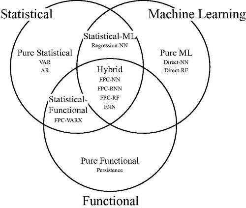
We focus on hybrid FPC-ML models over other types of FNNs because traditional ML structures for vector-based inputs can be directly used. Because ML methods already require various tuning steps and hyperparameter selection, using FPC-ML models can reduce the complexity of incorporating ML into applied ecological forecasting. Some concerns with FPC-ML methods, such as the arbitrary pre-selection of basis functions and the failure of FPC dimension reduction to incorporate information from the output (Yao et al. 2021) are mitigated in our work by our use of a saturated basis and lagged values of the independent variable. Therefore, we compare FPC-based hybrid models (FPC-NN, FPC-RNN, and FPC-RF) with the statistical-functional approach (FPC-VARX) and purely ML models (Direct-NN and Direct-RF). A purely functional Persistence model serves as a baseline comparison. Figure 1 illustrates the relationship between the models mentioned in this paper and their respective paradigms.

Figure 1. Schematic illustration of different categories of modeling approaches and their overlap. Hybrid models are those models in the center that have elements of both statistical and machine learning that incorporate the functional structure of the data.

From a data science perspective, this study investigates if hybrid FPC-ML methods are capable of accounting for complicated patterns and non-linearity in vertical DO profiles, and in doing so, provides the first statistical comparison of hybrid FPC-ML models with statistical-functional and pure ML methods. From a limnological and ecological perspective, this work introduces a new use of hybrid statistical-ML and RF models for DO lake profile functional forecasting, with the goal of motivating future exploration of ML techniques in the limnological community. This work is the first hybrid statistical-ML study to (1) implement function-to-function forecasting of complete profiles with exogenous variables, (2) introduce RF and recurrent NN extensions during the score forecast step, (3) provide simultaneous comparison against both a statistical-functional approach and purely ML approaches, and (4) build empirical prediction bands for all approaches.

The remainder of this paper is organized as follows: In Section 2, we outline the collection and pre-processing of the DO case study data. In Section 3, we describe the models and the forecasting algorithm. In Section 4, we compare the results of the models, and Section 5 offers concluding remarks regarding how to further improve models and how these models may be used in practice.

2. Case Study Data

From April 25, 2019 to October 29, 2019, a Hydrolab HL7 Multiparameter Datasonde capable of measuring water temperature, DO, pH, and electrical conductivity was utilized with an automated profiling system near the dam of Eagle Mountain Lake (EML). The percent saturation of DO was also recorded, which is the percentage of DO in the water relative to that expected in the atmosphere, and is the variable of interest for forecasting. The profiler moved the sonde from the surface (0.0 m) to near-bottom (10.0 m), collecting data every 0.5 m every 2 hours, resulting in twenty-one discrete depths measured per observation. The sonde was maintained every 1–2 weeks, depending on water temperature, with more frequent maintenance required at warmer temperatures. Sensors were assessed for instrument drift, cleaned, and recalibrated during each maintenance event. More details on the data collection, imputation of a small percentage of missing data (less than 4%), and variable definitions can be found in Durell et al. (2022). Figure 2 displays the location of EML and the profiler.

Figure 2. Location of Eagle Mountain Lake in Texas. The red dot designates the location of the profiler. Source: https://waterdatafortexas.org/reservoirs/individual/eagle-mountain/location.png.

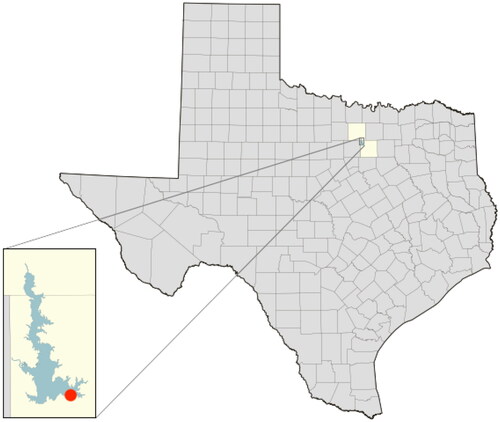
Forecasting DO profiles in EML has important ecological implications. Tarrant Regional Water District (TRWD) manages EML along with multiple other reservoirs in the Dallas Fort-Worth area. Forecasting DO in each reservoir could enable TRWD to adaptively draw water from different reservoirs based on forecast conditions. They could also make water-body specific choices about depth and time of day for collection. Furthermore, EML is a shallow, polymictic lake. When the lake mixes, the entire lake becomes nearly hypoxic, putting stress on the fish and other aquatic biota. Researchers may be interested in studying this hypoxia-induced stress and identifying the hypoxia threshold at which fish kills are initiated in a specific water body. Because it is not known when the lake will mix, DO profile forecasts could be used to identify early mixing and trigger the collection of data.

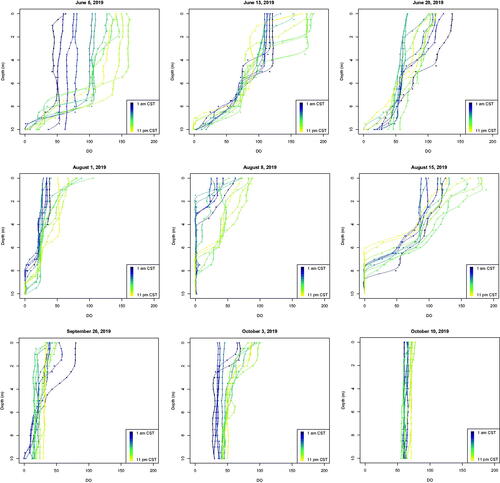
For each variable recorded by the sonde, the 21-dimensional vectors are smoothed using penalized, saturated B-spline basis functions with a roughness penalty chosen by generalized cross validation as outlined in Kokoszka and Reimherr (2017). Figure 3 displays the results of this smoothing approach for DO. The vertical axis designates lake depth where 0 m corresponds to the surface and 10 m corresponds to the bottom of the lake. Each panel shows twelve observations on a given day, with colors ranging from dark purple at the beginning of the day (1 am CST) to bright gold at the end of the day (11 pm CST). Here, each panel shows one full day's observations, selected from a week in early summer, late summer, or fall. The points show the observed measurements at each depth, and the corresponding line is the smoothed approximation. Visually, it appears that generalized cross validation provides a balance between a smooth fit and interpolation of the points. The figure reveals that the observations contain temporal dependence in that for a given day, observations of similar color are closer together and more similarly shaped. However, there is also clear seasonal variation in the data as the overall shape of the functions can differ dramatically.

Figure 3. Profile plots of the smoothed vertical measurements of DO, showing one day’s observations for a selection of weeks. The colors indicate the hour of the day and progress from dark purple (1 am CST) to light gold (11 pm CST).

3. Methodology

3.1. Hourly Centering

To address the diurnal dependence demonstrated in Figure 3, the observations are first centered by their corresponding hourly sample means. As will be discussed in Section 3.5, a rolling window is employed to minimize the effect of seasonal variation. Thus, the hourly means are re-estimated for each window. We present the methodology in terms of centered data, but plot the forecasts and true curves with the sample hourly means added back.

3.2. Functional Principal Component Analysis (FPCA)

Let $Y_n(s),n=1,\dots ,N$ denote a mean-zero, stationary functional time series of square integrable functions such that $\int Y_n^2(s)ds<\infty$ and $s\in [S_1,S_2].$ The goal is to obtain a forecast for the unobserved h-step-ahead curve, $Y_{N+h}(s).$ One established approach is to implement a truncated Karhunen-Loève approximation, (4) $$Y_n(s)\approx \sum _{j=1}^d{\xi }_{n,j}{\nu }_j(s),$$(4) where ${\nu }_j(s)$ is the jth FPC, defined as the jth eigenfunction of the covariance function, $c(s,s\prime )=E[Y_n(s)Y_n(s\prime )],$ ordered by decreasing eigenvalues (Kokoszka and Reimherr 2017). That is, ${\nu }_1(s)$ describes the most variability among the set $\{Y_1(s),\dots ,Y_N(s)\};$ ${\nu }_2(s)$ the second most; and so on. The jth FPC score is denoted ${\xi }_{n,j}=〈Y_n,{\nu }_j〉=\int Y_n(s){\nu }_j(s)ds.$ The truncation level, d, is the number of FPCs chosen. When d is allowed to approach infinity, the approximation in Equation 4(4) $$Y_n(s)\approx \sum _{j=1}^d{\xi }_{n,j}{\nu }_j(s),$$(4) is replaced with an equality.

In practice, a sample of centered curves, $\{Y_1(s),\dots ,Y_N(s)\}$ can be used to compute the sample covariance function as $\widehat{c}(s,s\prime )=\frac{1}{N}{\sum }_{n=1}^N{Y}_n(s)Y_n(s\prime ).$ Then, the d-dimensional vector of empirical FPCs (EFPCs), ${\mathit{\nu }}^e=({\nu }_1^e,\dots ,{\nu }_d^e)\prime ,$ and d-dimensional vectors of empirical scores, ${\mathit{\xi }}_n^e=({\xi }_{n,1}^e,\dots ,{\xi }_{n,d}^e)\prime$ for $n=1,\dots ,N$ are computed. The N score vectors and any exogenous variables, which can be scalar-valued, vector-valued variables, or FPC scores from other functional variables, can be fit with a suitable model to forecast the h-step ahead vector of EFPC scores, ${\mathit{\xi }}_{N+h}^e.$ Finally, the forecast score vector, ${\widehat{\mathit{\xi }}}_{N+h}^e,$ can be used directly to construct a forecast for $Y_{N+h}(s)$ as follows (5) $${\widehat{Y}}_{N+h}(s)=({\widehat{\mathit{\xi }}}_{N+h}^e)\prime {\mathit{\nu }}^e.$$(5)

3.3. Models

For the FPC-based models, $Y_n(s)$ denotes the nth smoothed functional observation of DO with ${\mathit{\xi }}_n^e$ as the corresponding EFPC score vector of dimension d. We denote the EFPC score vectors for the three functional exogenous variables, temperature, conductivity, and pH as ${\mathit{\gamma }}_{n,1}^e,{\mathit{\gamma }}_{n,2}^e,$ and ${\mathit{\gamma }}_{n,3}^e$ of dimension $d_{{\gamma }_1},d_{{\gamma }_2},$ and $d_{{\gamma }_3},$ respectively. The choices of $d,d_{{\gamma }_1},d_{{\gamma }_2},$ and $d_{{\gamma }_3}$ are critical, and many methods exist to aid in selecting these values. One common approach is to select the smallest dimension such that the cumulative variance explained meets a threshold (Wang et al. 2020). A data-driven method based on a functional final prediction error is presented in Aue et al. (2015). In the supplementary materials of Durell et al. (2022), these strategies were compared to a selection of $d=10,d_{{\gamma }_1}=2,d_{{\gamma }_2}=2,$ and $d_{{\gamma }_3}=3,$ chosen by visual inspection. The visual selection resulted in better forecasts for the EML data in terms of RMSE, so we retain the same choice for this study.

In the following sections, we present the technical details of all the models in terms of the dimensions and variables of the EML data, with the hope of clearly outlining the fitting procedures and encouraging reproducibility and adoption in similar studies. They are a purely functional approach (Persistence); two purely ML approaches (Direct-NN, Direct-RF); a statistical-functional approach (FPC-VARX); and three hybrid FPC-ML models: a basic feedforward NN (FPC-NN), a recurrent NN (FPC-RNN), and an RF (FPC-RF). The process used to select hyperparameters for the NN and RF-based methods is discussed in the Supplementary Material for this article.

3.3.1. Persistence

The Persistence model selects the current, uncentered functional observation of DO as the h-step-ahead forecast. This is a common baseline model and can be thought of as a “best guess” for future DO conditions that do not require sophisticated modeling or expert knowledge.

3.3.2. Direct Neural Network (Direct-NN)

The purely ML Direct-NN model relies on the raw, 21-dimensional vectors of DO, ${\mathbf{y}}_n=(Y_n(s_1),\dots ,Y_n(s_{21}))\prime ,n=1,\dots ,N.$ The Direct-NN takes as input a stacked vector, ${\mathbf{z}}_{n-h},$ of lag h vector-valued observations of DO and any desired exogenous variables. More than one lagged value can be used, but Durell et al. (2022) found that in general, no improvement in forecast RMSE resulted from including multiple lags, so we consider the following methods with a single lagged input.

When no exogenous variables are included, ${\mathbf{z}}_{n-h}={\mathbf{y}}_{n-h}.$ Otherwise, if ${\mathbf{x}}_{n,1},{\mathbf{x}}_{n,2},$ and ${\mathbf{x}}_{n,3}$ are the 21-dimensional vectors of temperature, conductivity, and pH, respectively, then we have an 84-dimensional input vector, ${\mathbf{z}}_{n-h}=({\mathbf{y}}_{n-h},{\mathbf{x}}_{n-h,1},{\mathbf{x}}_{n-h,2},{\mathbf{x}}_{n-h,3})\prime .$ For a Direct-NN with J layers, the first hidden layer is defined as (6) $${\mathbf{h}}_{n-h,1}={\varphi }_1({\mathbf{W}}_1{\mathbf{z}}_{n-h}+{\mathbf{b}}_1),$$(6) the jth layer as (7) $${\mathbf{h}}_{n-h,j}={\varphi }_j({\mathbf{W}}_j{\mathbf{h}}_{n-h,j-1}+{\mathbf{b}}_j),$$(7) and the output layer as, (8) $${\mathbf{y}}_n={\mathbf{W}}_J{\mathbf{h}}_{n-h,J}+{\mathbf{b}}_J+{\mathbf{\epsilon }}_n,$$(8) where ${\varphi }_j(·)$ is the jth activation function; the parameters to be estimated with a gradient-descent-based optimizer are ${\mathbf{W}}_j$ and ${\mathbf{b}}_j$ for $j=1,\dots ,J;$ and ${\mathbf{\epsilon }}_n$ is a 21 × 1 mean-zero error vector. This model is fit to ${\mathbf{z}}_1,\dots ,{\mathbf{z}}_N$ to obtain a forecast, ${\widehat{\mathbf{y}}}_{N+h}.$ To compare this model’s forecasts with the functional methods, penalized B-spline smoothing is applied to ${\widehat{\mathbf{y}}}_{N+h}$ to obtain a smooth functional forecast, ${\widehat{Y}}_{N+h}(s).$

3.3.3. Direct Random Forest (Direct-RF)

A random forest model is built by averaging the results of a collection of T decision trees. First, we denote a matrix of inputs as $\mathbf{Z}$ with each row corresponding to an input vector as defined in Section 3.3.2, ${\mathbf{z}}_n,n=1,\dots ,N-h.$ If no exogenous variables are used, the dimensions of $\mathbf{Z}$ are $(N-h)\times 21$ and otherwise are $(N-h)\times 84.$ We forecast one depth of the function at a time. For a fixed depth, $s_p,p=1,\dots ,21,$ we define the output vector as ${\mathbf{y}}^p=(Y_{h+1}(s_p),\dots ,Y_N(s_p))\prime .$

The tth decision tree for $t=1,\dots ,T$ is fit by first creating a bootstrapped data set denoted by ${\mathbf{Z}}^t$ and ${\mathbf{y}}^{p,t},$ where ${\mathbf{Z}}^t$ is constructed by sampling N – h times with replacement from the rows of $\mathbf{Z},$ and ${\mathbf{y}}^{p,t}$ are the corresponding resampled elements of ${\mathbf{y}}^p.$ Then, recursive binary splitting as defined in Hastie et al. (2009) is performed with a random subset of the columns from ${\mathbf{Z}}^t,$ typically of size equal to the square root of the number of columns of ${\mathbf{Z}}^t,$ to partition the 21-dimensional or 84-dimensional input space into R regions, ${\mathcal{R}}_r,r=1,\dots ,R.$ The choice of T, R, and the size of the subset of inputs can be pre-specified based on computational requirements or selected with cross validation.

We identify the constructed region, ${\mathcal{R}}_r,$ that corresponds to values of the forecast input data, ${\mathbf{z}}_N,$ and denote the region ${\mathcal{R}}_z.$ Then, ${\mathbf{y}}_{{\mathcal{R}}_z}^{p,t,i}$ denotes the ith element of an $N_{{\mathcal{R}}_z}$-dimensional vector, where $N_{{\mathcal{R}}_z}$ denotes the number of elements of ${\mathbf{y}}^{p,t}$ that have associated predictor variables that fall into ${\mathcal{R}}_z.$ Then, we can define the tth forecast for the pth depth as ${\widehat{Y}}_{N+h}^t(s_p)=\frac{1}{N_{{\mathcal{R}}_z}}{\sum }_{i=1}^{N_{{\mathcal{R}}_z}}{\mathbf{y}}_{{\mathcal{R}}_z}^{p,t,i}.$ The random forest is obtained by repeating this process for T trees and obtaining a forecast for the pth depth as ${\widehat{Y}}_{N+h}(s_p)=\frac{1}{T}{\sum }_{t=1}^T{\widehat{Y}}_{N+h}^t(s_p).$ A random forest is fit for each depth to obtain a final forecast vector, ${\widehat{\mathbf{y}}}_{N+h}=({\widehat{Y}}_{N+h}(s_1),\dots ,{\widehat{Y}}_{N+h}(s_{21}))\prime .$ As with the Direct-NN, penalized B-spline smoothing is used to smooth ${\widehat{\mathbf{y}}}_{N+h}$ to obtain ${\widehat{Y}}_{N+h}(s).$

3.3.4. Vector Autoregressive with Exogenous Variables (FPC-VARX)

The statistical-functional FPC-VARX model is a VARX of order one applied to the FPC scores. The FPC-VARX model incorporates the exogenous variables as a stacked vector of their scores, denoted ${\mathit{\gamma }}_{n-h}^{*}=({\mathit{\gamma }}_{n-h,1}^e,{\mathit{\gamma }}_{n-h,2}^e,{\mathit{\gamma }}_{n-h,3}^e)\prime ,$ of dimension ${\sum }_{i=1}^3{d}_{{\gamma }_i}.$ The model is (9) $${\mathit{\xi }}_n^e=\mathbf{c}+\mathbf{A}{\mathit{\xi }}_{n-h}^e+\mathbf{B}{\mathit{\gamma }}_{n-h}^{*}+{\mathbf{\epsilon }}_n,$$(9) where $\mathbf{c}$ is a $d\times 1$ vector of constants; $\mathbf{A}$ and $\mathbf{B}$ are d × d and $d\times {\sum }_{i=1}^3{d}_{{\gamma }_i}$ coefficient matrices, respectively; and ${\mathbf{\epsilon }}_n$ is a $d\times 1$ mean-zero random error vector.

The FPC-ML methods require the scores from all variables to be stacked into one vector, and the FPC-VARX model can be rewritten in this same format. Let ${\mathit{\xi }}_{n-h}^{*}$ be a stacked vector of FPC scores from all variables. When temperature, conductivity, and pH are used, ${\mathit{\xi }}_{n-h}^{*}=({\mathit{\xi }}_{n-h}^e,{\mathit{\gamma }}_{n-h,1}^e,{\mathit{\gamma }}_{n-h,2}^e,{\mathit{\gamma }}_{n-h,3}^e)\prime =({\mathit{\xi }}_{n-h}^e,{\mathit{\gamma }}_{n-h}^{*})\prime$, and when no exogenous variables are included, ${\mathit{\xi }}_{n-h}^{*}={\mathit{\xi }}_{n-h}^e.$ Then, the model in Equation 9(9) $${\mathit{\xi }}_n^e=\mathbf{c}+\mathbf{A}{\mathit{\xi }}_{n-h}^e+\mathbf{B}{\mathit{\gamma }}_{n-h}^{*}+{\mathbf{\epsilon }}_n,$$(9) can be written as (10) $${\mathit{\xi }}_n^e=\mathbf{c}+{\mathbf{A}}^{*}{\mathit{\xi }}_{n-h}^{*}+{\mathbf{\epsilon }}_n,$$(10) where ${\mathbf{A}}^{*}=\mathbf{A}$ when only DO is used, and ${\mathbf{A}}^{*}=[\mathbf{A},\mathbf{B}]$ is a $d\times (d+{\sum }_{i=1}^3{d}_{{\gamma }_i})$ coefficient matrix when exogenous variables are included. The parameters $\mathbf{c}$ and ${\mathbf{A}}^{*}$ are both estimated with ordinary least squares. The score forecast step is ${\widehat{\mathit{\xi }}}_{N+h}^e=\widehat{\mathbf{c}}+{\widehat{\mathbf{A}}}^{*}{\mathit{\xi }}_N^{*}.$

3.3.5. FPC Feedforward Neural Network (FPC-NN)

The FPC-NN is a fully connected feedforward neural network constructed as in Section 3.3.2 with the modification that the input and output vectors are the FPC scores as defined in Sections 3.2 and 3.3.4. That is, the FPC-NN is fit using the stacked vectors ${\mathit{\xi }}_1^{*},\dots ,{\mathit{\xi }}_{N-h}^{*}$ as inputs and ${\mathit{\xi }}_{h+1}^e,\dots ,{\mathit{\xi }}_N^e$ as outputs. When using J hidden layers, the first hidden layer is defined as (11) $${\mathbf{h}}_{n-h,1}={\varphi }_1({\mathbf{W}}_1{\mathit{\xi }}_{n-h}^{*}+{\mathbf{b}}_1),$$(11) the jth layer is given as in Equation 7(7) $${\mathbf{h}}_{n-h,j}={\varphi }_j({\mathbf{W}}_j{\mathbf{h}}_{n-h,j-1}+{\mathbf{b}}_j),$$(7) , and the output layer is, (12) $${\mathit{\xi }}_n^e={\mathbf{W}}_J{\mathbf{h}}_{n-h,J}+{\mathbf{b}}_J+{\mathbf{\epsilon }}_n.$$(12)

The fitted model then can be used to obtain a forecast, ${\widehat{\mathit{\xi }}}_{N+h}^e,$ which can be directly used in Equation 5(5) $${\widehat{Y}}_{N+h}(s)=({\widehat{\mathit{\xi }}}_{N+h}^e)\prime {\mathit{\nu }}^e.$$(5) . Graphically, the structure of the FPC-NN is shown in Figure S1 of the Supplementary Material.

3.3.6. Recurrent Neural Network (FPC-RNN)

The FPC-RNN is a recurrent neural network that is very similar to the FPC-NN, except that the first hidden layer directly depends on past hidden layers. That is, (13) $${\mathbf{h}}_{n-h,1}={\varphi }_1({\mathbf{W}}_1{\mathit{\xi }}_{n-h}^{*}+\mathbf{V}{\mathbf{h}}_{n-h-1}+{\mathbf{b}}_1).$$(13)

The only differences between Equations 11(11) $${\mathbf{h}}_{n-h,1}={\varphi }_1({\mathbf{W}}_1{\mathit{\xi }}_{n-h}^{*}+{\mathbf{b}}_1),$$(11) and 13(13) $${\mathbf{h}}_{n-h,1}={\varphi }_1({\mathbf{W}}_1{\mathit{\xi }}_{n-h}^{*}+\mathbf{V}{\mathbf{h}}_{n-h-1}+{\mathbf{b}}_1).$$(13) are the introduction of ${\mathbf{h}}_{n-h-1}$ and the weight matrix $\mathbf{V},$ which is estimated along with the other weight matrices and biases. Incorporating previously hidden layers could allow the model to better capture the temporal structure of the data. Graphically, the structure of the FPC-RNN is shown in Figure S2 of the Supplementary Material.

3.3.7. FPC Random Forest (FPC-RF)

The FPC-RF is a random forest constructed as in Section 3.3.3 except that the FPC scores, $\{{\mathit{\xi }}_1^{*},\dots ,{\mathit{\xi }}_{N-h}^{*}\}$ and $\{{\mathit{\xi }}_{h+1}^e,\dots ,{\mathit{\xi }}_N^e\},$ are used to construct the respective inputs and outputs. The elements of ${\mathit{\xi }}_{N+h}^e=({\xi }_{N+h,1}^e,\dots ,{\xi }_{N+h,d}^e)\prime$ are forecast independently, compiled into a forecast score vector ${\widehat{\mathit{\xi }}}_{N+h}^e,$ and used in Equation 5(5) $${\widehat{Y}}_{N+h}(s)=({\widehat{\mathit{\xi }}}_{N+h}^e)\prime {\mathit{\nu }}^e.$$(5) to obtain a forecast of DO.

3.3.8. Discussion of the Proposed Models

While direct methods like Direct-NN and Direct-RF are simpler to employ and understand than the FPC-based methods, the high dimensional input collected with measurement error could impair the performance of these methods. The FPC-based methods do require the additional pre-processing step of FPCA, but otherwise they are attractive for a variety of reasons. First, they result in a lower dimensional input, which is particularly important because as the technology for vertical profile data improves, the vertical density of the data collected will increase. Furthermore, transforming to the lower dimensional space will eliminate some measurement error and noise. Second, the FPCA step transforms each variable into a vector of independent elements, which may not be necessary for the ML-based methods, but it does typically simplify modeling. Finally, while we have not explored this option, modeling the functions as observations allows for potentially relevant first or second derivatives of the functions to be included.

Statistical methods like FPC-VARX are desirable for their speed and interpretability. Speed is a concern for short-term limnological forecasting, and statistical approaches like FPC-VARX are markedly faster than ML-based methods. In our application, all of the methods can produce forecasts on the order of seconds, but statistical methods may be needed if prediction bands are desired, which take much longer to compute. The VARX model and its special cases, such as AR and ARX, are also well-established. They have the ability to directly incorporate information across depths and temporal lags in the empirical FPC scores.

Feedforward NNs have a history of good performance and are a standard ML method in the scientific literature. RNNs are less frequently employed, but they are important for time-series forecasting because they take advantage of lagged layers and allow historical information to propagate through the fitting process. A major challenge with NNs and RNNs is the need to select hyperparameters, which can be overwhelming and arbitrary without expert knowledge. For ecological practitioners to adopt ML methods, they should provide insight on the process and also be computationally feasible. In light of this, we feel that RFs may be a better standard model for ecological forecasting because they involve fewer tuning decisions, have an intuitive structure, and are straightforward to implement.

3.4. Functional Prediction Bands

Functional prediction bands for stationary data are computed according to the method presented in Section 5.2 of Aue et al. (2015). In the following, we describe this approach in terms of our notation. Scalar parameters, β₁ and β₂, must be estimated such that (14) $$P({\widehat{Y}}_{N+h}(s)-{\beta }_1\tau (s)\le Y_{N+h}(s)\le {\widehat{Y}}_{N+h}(s)+{\beta }_2\tau (s)\mathrm{ }\text{for}\mathrm{ }\text{all}\mathrm{ }s\in [S_1,S_2])=1-\alpha ,$$(14) for a given significance level, $\alpha \in (0,1),$ and positive function, $\tau (s).$

For $\mathcal{l}=L,\dots ,N-1,$ the observations $Y_{\mathcal{l}+h}(s)$ are forecast by fitting a model to the set of observations $\{Y_1(s),\dots ,Y_{\mathcal{l}}(s)\}$ where L is the smallest sample size used to fit the model. After obtaining ${\widehat{Y}}_{\mathcal{l}+h}(s)$ for each $\mathcal{l},$ the functional residuals, ${\widehat{\epsilon }}_{\mathcal{l}+h}(s)=Y_{\mathcal{l}+h}(s)-{\widehat{Y}}_{\mathcal{l}+h}(s),$ are computed. Next, estimates of ${\widehat{\beta }}_1$ and ${\widehat{\beta }}_2$ are constructed such that $100\times (1-\alpha )\%$ of ${\widehat{\epsilon }}_{\mathcal{l}+h}(s)$ satisfies (15) $$-{\widehat{\beta }}_1\widehat{\tau }(s)\le {\widehat{\epsilon }}_{\mathcal{l}+h}(s)\le {\widehat{\beta }}_2\widehat{\tau }(s)\mathrm{ }\text{for}\mathrm{ }\text{all}\mathrm{ }s\in [S_1,S_2],$$(15) where $\widehat{\tau }(s)$ is the sample standard deviation of $\{{\widehat{\epsilon }}_{L+h}(s),\dots ,{\widehat{\epsilon }}_{N-1+h}(s)\}.$ Assuming $Y_n(s),\hspace{0.17em}n=1,\dots ,N,$ are stationary, Aue et al. (2015) state that if L is large enough, approximate stationarity for ${\widehat{\epsilon }}_{\mathcal{l}+h}(s),\hspace{0.17em}\mathcal{l}=L,\dots ,N-1,$ can be expected. By a law of large numbers, (16) $$\frac{1}{N-L}\sum _{\mathcal{l}=L}^{N-1}I\left(-{\widehat{\beta }}_1\widehat{\tau }(s)\le {\widehat{\epsilon }}_{\mathcal{l}+h}(s)\le {\widehat{\beta }}_2\widehat{\tau }(s)\mathrm{ }\text{for}\mathrm{ }\text{all}\mathrm{ }s\in [S_1,S_2]\right),$$(16) is approximately equal to Equation 14(14) $$P({\widehat{Y}}_{N+h}(s)-{\beta }_1\tau (s)\le Y_{N+h}(s)\le {\widehat{Y}}_{N+h}(s)+{\beta }_2\tau (s)\mathrm{ }\text{for}\mathrm{ }\text{all}\mathrm{ }s\in [S_1,S_2])=1-\alpha ,$$(14) . Thus, the $100\times (1-\alpha )\%$ prediction bands are constructed as $({\widehat{Y}}_{N+h}(s)-{\widehat{\beta }}_1\widehat{\tau }(s),{\widehat{Y}}_{N+h}(s)+{\widehat{\beta }}_2\widehat{\tau }(s)).$ However, Aue et al. (2015) neither specify how to select L nor report empirical coverage for this method, so we explore different values of L and report the empirical coverages in Section 4.2 for all seven models.

3.5. Forecast Approach

Here, we summarize the forecasting algorithm. To address seasonal variation, we train models using a rolling window, where 5 weeks worth of observations are used to forecast a single h-step-ahead observation, and then the window rolls forward by dropping the first observation and adding the next observation. A window of 5 weeks is used based on prior work (Durell et al. 2022). We are interested in forecasting both 2 hours ahead (h = 1) and one day ahead (h = 12), which are both useful horizons for environmental and water treatment applications. Two different variable combinations are used: models with only lagged values of DO and models that also include all of the lagged exogenous variables: temperature, conductivity, and pH. For each combination of forecast horizon and variables (D or DTCpH, where D corresponds to the model with DO alone, and DTCpH refers to the model with all variables), we perform the steps below for $m=1,2,\dots ,M$ windows, where m indexes the current window.

3.6. Forecasting Algorithm

1. Set Window: Set m = 1.

2. Preprocess Data:

   1. Smooth the observed data using penalized B-spline smoothing.

   2. Remove diurnal trends from the data by estimating and subtracting the hourly means based on the observations in window m to obtain the 21-dimensional vectors $\{{\mathbf{y}}_1,\dots ,{\mathbf{y}}_N\}$ and the smoothed curves $\{Y_1(s),\dots ,Y_N(s)\}.$

   3. Perform FPCA on the detrended data to obtain ${\mathit{\nu }}^e$ and $\{{\mathit{\xi }}_1^e,\dots ,{\mathit{\xi }}_N^e\}.$

   4. If using exogenous variables (DTCpH), perform Steps 2a through 2c to obtain the EFPC scores of the exogenous variable versions of $\{{\mathbf{z}}_1,\dots ,{\mathbf{z}}_N\}$ and $\{{\mathit{\xi }}_1^{*},\dots ,{\mathit{\xi }}_N^{*}\}.$

3. Fit Models:

   1. Fit the Direct-NN and Direct-RF models using $\{{\mathbf{z}}_1,\dots ,{\mathbf{z}}_N\}$ to obtain a forecast vector, ${\widehat{\mathbf{y}}}_{N+h},$ for each method. Smooth the resulting vector using penalized B-spline smoothing to obtain ${\widehat{Y}}_{N+h}(s)$ for both methods.

   2. Fit the FPC-VARX, FPC-NN, FPC-RNN, and FPC-RF models to obtain a forecast score, ${\widehat{\mathit{\xi }}}_{N+h}^e,$ for each method. Apply Equation 5(5) $${\widehat{Y}}_{N+h}(s)=({\widehat{\mathit{\xi }}}_{N+h}^e)\prime {\mathit{\nu }}^e.$$(5) using the EFPCs obtained in Step 2c to obtain ${\widehat{Y}}_{N+h}(s)$ for each method.

4. Build Prediction Bands: If desired, obtain prediction bands according to Section 3.4.

5. Evaluate Models: For each model’s forecast, compute and store the functional root mean squared error as $\mathit{RMS}{E}_m=\sqrt{〈Y_{N+h}-{\widehat{Y}}_{N+h},Y_{N+h}-{\widehat{Y}}_{N+h}〉}.$

6. Cycle Through Windows: Update $m=m+1,$ and repeat Steps 2 through 5 until m = M.

7. Evaluate Overall Results: For each model, compute the overall root mean squared error $\mathit{RMSE}=\frac{1}{M}{\sum }_{m=1}^{M}RMS{E}_m.$

4. Results

4.1. Forecast Comparison

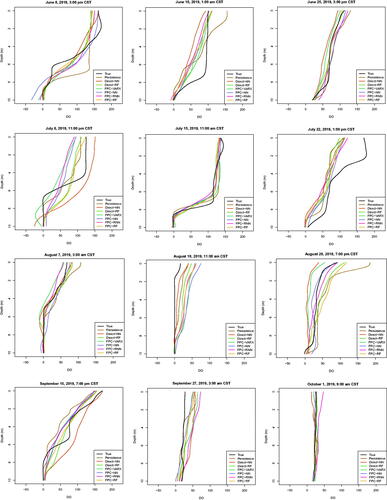
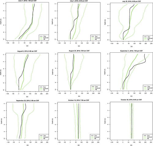
A selection of the day-ahead forecast results for the seven models using all exogenous variables can be viewed in Figure 4. It demonstrates the following: (1) The forecasts tend to do poorly when the true observation has sharp bends. (2) The forecasts appear to do better in the fall months due to the less variable profiles. (3) The bottom of the lake corresponds to lower forecast variability. That is, the forecast variability tends to increase as DO increases closer to the surface of the lake.

Figure 4. Profile plots of a selection of day-ahead forecasts using all exogenous variables and plotted with the corresponding true curve.

The RMSE results are outlined in Table 2. The overall RMSE is computed as well as seasonal RMSEs, where RMSEs from forecasts in the early summer (May-June), late summer (July-August), and early fall (September-October) are averaged. Forecasts are most accurate in the early fall and least accurate in the late summer. This is because in the early fall, the lake begins to mix, and the profiles become more vertical, making them easier to forecast.

Table 2. Forecasting results in terms of RMSE.

h	Variable Set	Model	Early Summer	Late Summer	Early Fall	Overall (Rank)
1	D	Persistence	11.32	12.70	7.66	10.43 (4)
		Direct-NN	11.16	12.18	8.22	10.41 (3)
		Direct-RF	10.82	11.65	8.08	10.07 (2)
		FPC-VARX	10.51	11.41	7.77	9.79 (1)
		FPC-NN	11.40	12.19	8.31	10.49 (5)
		FPC-RNN	14.66	15.01	11.31	13.46 (7)
		FPC-RF	11.42	12.61	8.71	10.83 (6)
	DTCpH	Persistence	11.32	12.70	7.66	10.43 (2)
		Direct-NN	11.77	12.87	8.98	11.11 (6)
		Direct-RF	11.66	12.43	8.65	10.77 (4)
		FPC-VARX	10.65	11.49	7.83	9.87 (1)
		FPC-NN	11.48	12.33	8.33	10.57 (3)
		FPC-RNN	13.88	14.08	10.93	12.78 (7)
		FPC-RF	11.38	12.68	8.63	10.82 (5)
12	D	Persistence	26.54	25.61	17.88	22.66 (7)
		Direct-NN	22.45	24.63	17.43	21.36 (5)
		Direct-RF	19.88	22.67	16.16	19.57 (1)
		FPC-VARX	21.54	23.60	16.55	20.41 (3)
		FPC-NN	21.56	23.43	17.15	20.58 (4)
		FPC-RNN	22.65	24.30	17.70	21.36 (5)
		FPC-RF	20.50	23.26	16.86	20.21 (2)
	DTCpH	Persistence	26.54	25.61	17.88	22.66 (7)
		Direct-NN	21.46	21.53	15.81	19.21 (3)
		Direct-RF	18.24	18.41	12.77	16.11 (1)
		FPC-VARX	21.10	21.95	16.53	19.62 (4)
		FPC-NN	21.53	22.47	15.90	19.66 (5)
		FPC-RNN	22.67	22.68	16.76	20.29 (6)
		FPC-RF	18.45	19.60	14.34	17.28 (2)

Bold values indicate the best overall and seasonal models. A lower rank in the Overall column corresponds to a better model. The Persistence model is identical across variable sets but is repeated for reference.

Focusing first on the 2-hour-ahead forecasts (h = 1), we see that incorporating exogenous variables results in a marginal loss of performance for all models except the FPC-RNN and FPC-RF models. The FPC-VARX model is superior to the the purely ML models and the hybrid statistical-functional-ML models. In terms of overall RMSE, the FPC-VARX model with variable D results in a 6.1% reduction over the Persistence model, a 2.8% reduction over the best purely ML model, Direct-RF, and a 6.7% reduction over the best hybrid model, FPC-NN.

Next, for the day-ahead forecasts (h = 12), the RF-based models outperform the FPC-VARX and the NN-based models. In this case, including all of the exogenous variables improves forecasts, so for the variable set DTCpH, the Direct-RF and the FPC-RF models reduce the overall RMSE over the Persistence model by 28.9% and 23.7%, respectively; over the FPC-VARX method by 17.9% and 11.9%, respectively; and over the best NN-based model, FPC-NN, by 18% and 12.1%, respectively. The Direct-RF reduced RMSE over the FPC-RF by 6.8%. For the Direct-RF and FPC-RF models, incorporating exogenous variables reduces the overall RMSE by 17.7% and 14.5%, respectively, compared to the corresponding Direct-RF and FPC-RF models without exogenous variables. This finding agrees with the results in Durell et al. (2022) where exogenous variables become more useful for longer forecast horizons.

For both forecast horizons, the FPC-RNN and Direct-NN models generally perform the worst, and they only outperform Persistence for day-ahead forecasts. These models have the most parameters to estimate, so overfitting or poor model fit may be to blame. For day-ahead forecasting, the FPC-VARX model and the NN-based models are not competitive.

The day-ahead forecast is particularly important because it provides a larger window of time to mitigate any possible water quality issues. For these data, the Direct-RF is the model of choice for day-ahead forecasts in terms of RMSE reduction, but the FPC-RF’s functional framework can naturally address missing values and unequally spaced observations. Furthermore, the FPC-RF is equipped for direct extension to more sophisticated methods, like multivariate FPCs, which can easily incorporate exogenous variables measured over different domains. Finally, in light of the ecological goal to develop real-time forecasts, the FPC-RF may be optimal under certain circumstances. With the current selection of hyperparameters, the Direct-RF took twice as long to run (approximately fourteen seconds per forecast without prediction bands and two minutes with prediction bands) compared to the FPC-RF (approximately seven seconds per forecast without prediction bands and one minute with prediction bands) on the 2019 6-core MacBook Pro with 16 GB RAM used for this study. While this difference is negligible for our day-ahead forecasting application, depending on the choice of hyperparameters, computational machinery, and density of the measured data collected, the dimension reduction occurring in the FPCA step for FPC-RF could be an extremely important step in reducing training time.

4.2. Prediction Bands

Prediction band computation is vital in assisting lake management and researchers quantify forecast error. When a practitioner plots the forecast with the functional prediction band, it is clear that where the band is narrow, decisions can be made more confidently. For example, water treatment experts operating variable intake systems could use the forecast curve and prediction bands to reliably collect water at a depth with higher forecast DO. Computing prediction bands for all models in this study according to Section 3.4 for all combinations of all forecasts is too computationally intensive to implement. For example, if $N-L=50,$ which is the number of observations to forecast to estimate the standard deviation, it would take forty-nine days to compute prediction bands for every combination of models, variables, and forecast horizons. However, computing prediction bands for a single forecast takes at most five minutes, making it plausible to construct prediction bands in real time for our application.

In the following, 95% prediction bands are computed for all models both for day-ahead forecasts with all variables and 2-hour-ahead forecasts with D alone for the same set of 50 randomly selected forecasts. We consider the impact of the initial sample size, L, by choosing three values of L such that the respective number of forecasts to compute equals $N-L=20,N-L=50,$ and $N-L=80$ for all combinations of models and horizons. As L increases, the number of in-sample forecasts used per pair of prediction bands decreases.

Three metrics are considered to evaluate prediction band performance. The first metric, absolute coverage, is used to define the prediction band confidence level in Equation 14(14) $$P({\widehat{Y}}_{N+h}(s)-{\beta }_1\tau (s)\le Y_{N+h}(s)\le {\widehat{Y}}_{N+h}(s)+{\beta }_2\tau (s)\mathrm{ }\text{for}\mathrm{ }\text{all}\mathrm{ }s\in [S_1,S_2])=1-\alpha ,$$(14) , and it measures the proportion of curves such that the true curve is completely contained within the prediction bands over the entire range. While an important metric, absolute coverage fails to consider the magnitude of the error when a curve exceeds the prediction bands. For example, the true curve may only exceed the prediction bands over a small range of depths, or the true curve may fall completely outside the entire prediction band range. In either case, the absolute coverage metric will classify both curves as “uncovered.” Thus, in order to further evaluate the prediction band behavior, we introduce a second, less conservative metric called the average coverage. This is defined as the proportion of the range of the true curve that is contained within the prediction bands, and then this value is averaged across all forecasts. In addition to the two coverage metrics, the overall width of the prediction bands is computed as the integral of the difference between the upper and lower bands and then averaged across all forecasts.

Table 3 displays the absolute coverage, the average coverage, and the average width of the prediction bands. The absolute coverage is less than 0.95 in every case; however, the average coverage indicates that the curves are only exceeding the prediction bands for a small range of depths. For both the absolute and average coverages, the day-ahead prediction bands generally have higher coverage than the 2-hour-ahead prediction bands. The empirical coverage also changes depending on L. For the day-ahead forecasts, $N-L=50$ appears to result in the highest coverage. For the width, as N – L increases, the interval width increases, except for the one-step-ahead persistence model. As expected, an increased width tends to correspond to higher coverage; however, in the h = 12 case, the choice of $N-L=50$ commonly results in both higher coverage and lower width than $N-L=80.$ This could imply that using a smaller pool of only the most recent forecasts provides an improved estimate of the standard deviation.

Table 3. Prediction band empirical coverage based on a random sample of 50 forecasts.

		Absolute coverage			Average coverage			Width
h	Model	20	50	80	20	50	80	20	50	80
1	Persistence	0.66	0.76	0.80	0.95	0.97	0.98	999	1013	965
	Direct-NN	0.72	0.80	0.84	0.94	0.97	0.98	574	712	782
	Direct-RF	0.70	0.78	0.86	0.94	0.97	0.98	594	724	786
	FPC-VARX	0.70	0.76	0.78	0.94	0.97	0.98	572	700	758
	FPC-NN	0.72	0.82	0.90	0.92	0.98	0.99	586	712	776
	FPC-RNN	0.76	0.84	0.84	0.95	0.97	0.97	691	807	860
	FPC-RF	0.68	0.78	0.82	0.94	0.98	0.98	598	726	784
12	Persistence	0.80	0.88	0.80	0.92	0.96	0.95	1246	1484	1548
	Direct-NN	0.76	0.86	0.90	0.94	0.97	0.99	932	1087	1170
	Direct-RF	0.74	0.86	0.86	0.94	0.97	0.96	796	965	1032
	FPC-VARX	0.80	0.88	0.88	0.96	0.98	0.98	986	1113	1173
	FPC-NN	0.80	0.90	0.84	0.94	0.98	0.97	942	1090	1152
	FPC-RNN	0.72	0.86	0.82	0.93	0.98	0.96	972	1148	1226
	FPC-RF	0.76	0.84	0.86	0.95	0.97	0.97	827	1007	1058

The 2-hour-ahead forecasts use D, and the day-ahead forecasts use DTCpH. Absolute coverage measures the proportion of times the entire curve is contained within the prediction bands. Average coverage measures the average proportion of the true curve contained within the prediction bands. Width is computed as the average of the integral of the difference between each upper and lower band pair within a given model. The results are displayed for three choices of N – L, namely 20, 50, and 80. Bold values indicate the L that results in highest coverage or lowest width.

Figure 5 displays an example of 95% prediction bands using $N-L=50$ for forecasts on August 8 at 7:00 pm. The plot displays 2-hour-ahead forecasts with D (top row) and day-ahead forecasts with DTCpH (bottom row). As expected, the prediction bands for the day-ahead forecasts are wider. Differences among models are more apparent for the day-ahead forecasts, where the FPC-NN and FPC-RNN models result in narrower bands, and the Persistence model results in wide bands for this specific forecast. Because the Direct-RF model has the best performance for day-ahead forecasts with DTCpH, we show 95% prediction bands for a selection of forecasts to investigate the seasonal prediction band behavior in Figure 6. The bands are widest during the late summer and most narrow during the fall. When the observation lies outside of the prediction band, such as the observation on September 3 at 7 pm, it is typically only over a small portion of the curve.

Figure 5. Profile plots of forecasts and prediction bands with the true curve for August 8, 2019 at 7 pm CST. The 2-hour-ahead forecasts (top row) use D alone and the day-ahead forecasts (bottom row) use DTCpH.

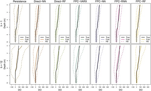
Figure 6. Eight profile plots of the true curve with the day-ahead Direct-RF forecast model with DTCpH and 95% prediction bands overlaid.

5. Conclusion

This study seeks to both investigate the benefits of hybrid FPC-ML methods and to contribute a detailed example of incorporating data-driven ML methods for functional forecasting of vertical DO profiles. In doing so, we explore the understudied framework of function-to-function forecasting with exogenous variables and, to our knowledge, provide the the first simultaneous comparison of hybrid FPC-ML methods with purely functional, purely ML, and functional-statistical FDA methods, allowing important insights into the strengths and weaknesses of the different approaches. It does not appear that more advanced ML techniques beyond fully connected feedforward NNs are frequently utilized in the current FPC-ML literature, so describing the use of RNNs and RFs in FPC-based functional time series forecasting is a marked advance. While there are examples of using RFs to predict DO, such as the use of monthly measurements of off-shore coastal vertical profiles (Valera et al. 2020), according to our literature review, this is the first application of a hybrid statistical-ML type of model and specifically an RF model for functional forecasting of DO lake profiles. Furthermore, prediction bands have not yet been applied for FPC-ML applications, and they are vital for decision making in water treatment and management. The methods and results presented in this article suggest that FPC-ML models may succeed in settings where traditional process-based hydrodynamic models produce unreliable forecasts of high-frequency time series data without prediction bands.

To accomplish our objectives, we demonstrate the steps needed to obtain forecast curves, including smoothing and centering the data, obtaining FPCs, forecasting scores, and computing functional prediction bands. Our results show that in functional forecasting of DO, context is important. As the forecast horizon increases, the performance of the purely-ML methods improves. If a short forecast horizon in terms of hours or minutes is desired, a simple and fast statistical-functional model like FPC-VARX could be preferable, and collection of exogenous data may not be needed. For longer forecast horizons, incorporating exogenous variables and ML methods may lead to improvement over the purely statistical-functional approach. What constitutes a short or a long horizon will be specific to the temporal dynamics of the particular application. We also find that while empirical absolute coverage for this prediction band method is low and sensitive to the choice of L, high average coverage suggests that the proportion of the observation that exceeds the prediction bands is typically quite small.

The superiority of Direct-RF over the hybrid FPC-RF model for the day-ahead forecasts in this application may be due to complex nonlinear dynamics propagating through the system as the horizon increases. It may be possible that blending the statistical and ML approaches with hybrid models results in optimal performance at some horizon between 2 and 24 hours ahead. In favor of the hybrid models, the inherent smoothing and dimension reduction steps could be particularly important in cases of large measurement error, vertically dense data collection, or missing data. Furthermore, as discussed in Section 4.1, the specific computational tools available and the desired choice of hyperparameters will vary by scientific context and will impact the speed and accuracy of the forecasts.

Interesting extensions to this work could explore the performance of other types of ML methods for ecological forecasting, such as long-short-term memory NNs or boosted trees. The multivariate functional principal components developed and implemented in Chiou et al. (2014), Happ and Greven (2018), and Wang et al. (2020) could be combined with the FPC-ML methods to potentially improve the impact of including exogenous variables. While this work did not consider the forecasting problem from a Bayesian paradigm, a variety of Bayesian methods could be explored. After the smoothing and FPCA steps, Bayesian linear models could be applied to the FPC scores in the bayeslm or rstanarm R packages (Gelman and Hill 2007; Gabry et al. 2022; He et al. 2022), but elicitation of a reasonable prior distribution for the FPC scores may be nontrivial. Furthermore, a hybrid Bayesian machine learning approach could consider Bayesian additive regression trees (BART) as applied to the FPC scores (Chipman et al. 2010). Other non-hybrid modeling approaches would also be of interest to explore, such as functional neural networks (Rao and Reimherr 2021) and functional BART (Starling et al. 2020).

In terms of data quality, future modeling would benefit from data that are measured over multiple years to incorporate seasonal effects. Additionally, high frequency (measured very often in time) and high density (measured over a fine grid spatially) data such as those used in this study are preferred for forecasting water quality profiles to allow for straightforward smoothing pre-processing. Lastly, future work should seek to take advantage of relevant scalar exogenous variables that measure atmospheric conditions, such as wind speed, solar radiation, and temperature. We hypothesize that incorporating these types of variables may make the greatest improvements in data-driven forecasts for DO lake profiles.

Acknowledgements

We would like to thank Dr. Alexander Aue, Professor, Department of Statistics, UC Davis who shared R code from Aue et al. (2015).

Additional information

Funding

This work was supported by the National Science Foundation Harnessing the Data Revolution: Data Science Corps project [#1924146] to ASH, with additional support from the Tarrant Regional Water District to JTS for the collection of the EML data.

References

- Andersen MR, de Eyto E, Dillane M, Poole R, Jennings E. 2020. 13 Years of storms: an analysis of the effects of storms on lake physics on the atlantic fringe of Europe. Water. 12(2):318.
- Angamuthu Chinnathambi R, Mukherjee A, Campion M, Salehfar H, Hansen TM, Lin J, Ranganathan P. 2018. A multi-stage price forecasting model for day-ahead electricity markets. Forecasting. 1(1):26–46.
- Aue A, Norinho DD, Hörmann S. 2015. On the prediction of stationary functional time series. J Am Stat Assoc. 110(509):378–392.
- Banks JL, Ross DJ, Keough MJ, Eyre BD, Macleod CK. 2012. Measuring hypoxia induced metal release from highly contaminated estuarine sediments during a 40 day laboratory incubation experiment. Sci Total Environ. 420:229–237.
- Barua S, Elhalawani H, Volpe S, Al Feghali KA, Yang P, Ng SP, Elgohari B, Granberry RC, Mackin DS, Gunn GB, et al. 2021. Computed tomography radiomics kinetics as early imaging correlates of osteoradionecrosis in oropharyngeal cancer patients. Front Artif Intell. 4:618469.
- Carey CC, Woelmer WM, Lofton ME, Figueiredo RJ, Bookout BJ, Corrigan RS, Daneshmand V, Hounshell AG, Howard DW, Lewis ASL, et al. 2022. Advancing lake and reservoir water quality management with near-term, iterative ecological forecasting. Inland Waters. 12(1):107–120.
- Chin CK, Mat D. A b A, Saleh AY. 2021. Hybrid of convolutional neural network algorithm and autoregressive integrated moving average model for skin cancer classification among Malaysian. IJ-AI. 10(3):707–716.
- Chiou J-M, Chen Y-T, Yang Y-F. 2014. Multivariate functional principal component analysis: a normalization approach. Statistica Sinica. 24(4):1571–1596.
- Chipman HA, George EI, McCulloch RE. 2010. BART: Bayesian additive regression trees. Ann Appl Stat. 4(1):266–298.
- da Rosa CE, de Souza MS, Yunes J, a. S, Proença LAO, M, Nery LE, Monserrat JM. 2005. Cyanobacterial blooms in estuarine ecosystems: characteristics and effects on Laeonereis acuta (Polychaeta, Nereididae). Mar Pollut Bull. 50(9):956–964.
- Das P, Naganna SR, Deka PC, Pushparaj J. 2020. Hybrid wavelet packet machine learning approaches for drought modeling. Environ Earth Sci. 79(10):1–18.
- Durell L, Scott JT, Nychka D, Hering AS. 2022. Functional forecasting of dissolved oxygen in high-frequency vertical lake profiles. Environmetrics. [16 p.]. doi:10.1002/env.2765
- Fard AK, Akbari-Zadeh M-R. 2014. A hybrid method based on wavelet, ANN and ARIMA model for short-term load forecasting. J Exp Theor Artif Intell. 26(2):167–182.
- Ferré L, Villa N. 2006. Multilayer perceptron with functional inputs: an inverse regression approach. Scand J Stat. 33(4):807–823.
- Gabry J, Ali I, Brilleman S, Buros Novik J, AstraZeneca, Trustees of Columbia University, Wood S, R Core Development Team, Bates D, Maechler M, et al. rstanarm: Bayesian applied regression modeling via Stan. R package version 2.21.3. https://mc-stan.org/rstanarm/
- Gelman A, Hill J. 2007. Data analysis using regression and multilevel/hierarchical models. 1st ed. New York: Cambridge University Press.
- Happ C, Greven S. 2018. Multivariate functional principal component analysis for data observed on different (dimensional) domains. J Am Stat Assoc. 113(522):649–659.
- Hastie T, Tibshirani R, Friedman J. 2009. The elements of statistical learning: data mining, inference, and prediction. 2nd ed. Springer Series in Statistics. New York: Springer-Verlag.
- He J, Hahn R, Lopes H, Herren A. 2022. bayeslm: efficient sampling for Gaussian linear regression with arbitrary priors. R package version 1.0.1. https://cran.ism.ac.jp/web/packages/bayeslm/bayeslm.pdf
- Hyndman RJ, Ullah MS. 2007. Robust forecasting of mortality and fertility rates: a functional data approach. Comput Stat Data Anal. 51(10):4942–4956.
- Ju X, Salibián-Barrera M. 2021. Tree-based boosting with functional data. arXiv:2109.02989 [stat].
- Karakaya N, Evrendilek F, Güngör K. 2011. Modeling and validating long-term dynamics of diel dissolved oxygen with particular reference to pH in a temperate shallow lake (Turkey). Clean Soil Air Water. 39(11):966–971.
- Kokoszka P, Reimherr M. 2017. Introduction to functional data analysis. Boca Raton (FL): Chapman and Hall/CRC.
- Lane SE, Robinson AP. 2011. An alternative objective function for fitting regression trees to functional response variables. Comput Stat Data Anal. 55(9):2557–2567.
- Lee JS, Zakeri IF, Butte NF. 2017. Functional data analysis of sleeping energy expenditure. PLOS One. 12(5):e0177286.
- Li H, Xiao G, Xia T, Tang YY, Li L. 2014. Hyperspectral image classification using functional data analysis. IEEE Trans Cybern. 44(9):1544–1555.
- Lin Z, Zhu H. 2019. MFPCA: multiscale functional principal component analysis. Proc AAAI Conf Artif Intell, 33(01):4320–4327.
- López M, Martínez J, Matí–As JM, Taboada J, Vilán JA. 2010. Functional classification of ornamental stone using machine learning techniques. J Comput Appl Math. 234(4):1338–1345.
- Meng Y, Liang J, Qian Y. 2016. Comparison study of orthonormal representations of functional data in classification. Knowledge Based Syst. 97:224–236.
- Mesman JP, Ayala AI, Adrian R, De Eyto E, Frassl MA, Goyette S, Kasparian J, Perroud M, Stelzer JAA, Pierson DC, et al. 2020. Performance of one-dimensional hydrodynamic lake models during short-term extreme weather events. Environ Model Software. 133:104852.
- Mohammadi B, Mehdizadeh S, Ahmadi F, Lien NTT, Linh NTT, Pham QB. 2021. Developing hybrid time series and artificial intelligence models for estimating air temperatures. Stoch Environ Res Risk Assess. 35(6):1189–1204.
- Nerini D, Ghattas B. 2007. Classifying densities using functional regression trees: applications in oceanology. Comput Stat Data Anal. 51(10):4984–4993.
- Newhart KB, Marks CA, Rauch-Williams T, Cath TY, Hering AS. 2020. Hybrid statistical-machine learning ammonia forecasting in continuous activated sludge treatment for improved process control. J Water Process Eng. 37:101389.
- Perdices D, de Vergara JEL, Ramos J. 2021. Deep-FDA: using functional data analysis and neural networks to characterize network services time series. IEEE Trans Netw Serv Manage. 18(1):986–999.
- Pesaresi S, Mancini A, Quattrini G, Casavecchia S. 2020. Mapping Mediterranean forest plant associations and habitats with functional principal component analysis using Landsat 8 NDVI time series. Remote Sens. 12(7):1132.
- Rahman R, Dhruba SR, Ghosh S, Pal R. 2019. Functional random forest with applications in dose-response predictions. Sci Rep. 9(1):1628.
- Rao AR, Reimherr M. 2021. Modern non-linear function-on-function regression. arXiv:2107.14151 [cs, stat].
- Rao AR, Wang Q, Wang H, Khorasgani H, Gupta C. 2020. Spatio-temporal functional neural networks. 2020 IEEE 7th International Conference on Data Science and Advanced Analytics (DSAA);81–89.
- Rossi F, Conan-Guez B. 2005. Functional multi-layer perceptron: a non-linear tool for functional data analysis. Neural Netw. 18(1):45–60.
- Rossi F, Conan-Guez B. 2006. Theoretical properties of projection based multilayer perceptrons with functional inputs. Neural Process Lett. 23(1):55–70.
- Rossi F, Conan-Guez B, Fleuret F. 2002. Functional data analysis with multi layer perceptrons. Proceedings of the 2002 International Joint Conference on Neural Networks. IJCNN’02 (Cat. No.02CH37290), Vol. 3; p. 2843–2848.
- Rossi F, Delannay N, Conan-Guez B, Verleysen M. 2005. Representation of functional data in neural networks. Neurocomputing. 64:183–210.
- Rossi F, Villa N. 2006. Support vector machine for functional data classification. Neurocomputing. 69(7-9):730–742.
- Siljic Tomic A, Antanasijevic D, Ristic M, Peric-Grujic A, Pocajt V. 2018. A linear and non-linear polynomial neural network modeling of dissolved oxygen content in surface water: inter- and extrapolation performance with inputs’ significance analysis. Sci Total Environ. 610–611:1038–1046.
- Starling JE, Murray JS, Carvalho CM, Bukowski RK, Scott JG. 2020. BART with targeted smoothing: an analysis of patient-specific stillbirth risk. Ann Appl Stat. 14(1):28–50.
- Tengberg A, Hovdenes J, Andersson HJ, Brocandel O, Diaz R, Hebert D, Arnerich T, Huber C, Körtzinger A, Khripounoff A, et al. 2006. Evaluation of a lifetime-based optode to measure oxygen in aquatic systems. Limnol Oceanogr Methods. 4(2):7–17.
- Thind B, Multani K, Cao J. 2022. Deep learning with functional inputs. J Comput Graph Stat.
- Thomas RQ, Figueiredo RJ, Daneshmand V, Bookout BJ, Puckett LK, Carey CC. 2020. A near-term iterative forecasting system successfully predicts reservoir hydrodynamics and partitions uncertainty in real time. Water Resour Res. 56(11):e2019WR026138.
- Valera M, Walter RK, Bailey BA, Castillo JE. 2020. Machine learning based predictions of dissolved oxygen in a small coastal embayment. JMSE. 8(12):1007.
- Wang Q, Farahat A, Gupta C, Zheng S. 2021. Deep time series models for scarce data. Neurocomputing. 456:504–518.
- Wang Q, Wang H, Gupta C, Rao AR, Khorasgani H. 2020. A non-linear function-on-function model for regression with time series data. 2020 IEEE International Conference on Big Data (Big Data); pages 232–239.
- Wang Q, Zheng S, Farahat A, Serita S, Gupta C. 2019. Remaining useful life estimation using functional data analysis. 2019 IEEE International Conference on Prognostics and Health Management (ICPHM); 1–8.
- Wang Q, Zheng S, Farahat A, Serita S, Saeki T, Gupta C. 2019. Multilayer perceptron for sparse functional data. 2019 International Joint Conference on Neural Networks (IJCNN); p. 1–10.
- Woelmer WM, Thomas RQ, Lofton ME, McClure RP, Wander HL, Carey CC. 2022. Near-term phytoplankton forecasts reveal the effects of model time step and forecast horizon on predictability. Ecol Appl. 32(7):e2642.
- Yao J, Mueller J, Wang JL. 2021. Deep learning for functional data analysis with adaptive basis layers. International Conference on Machine Learning; p. 11898–11908.
- Yu Y, Lambert D. 1999. Fitting trees to functional data, with an application to time-of-day patterns. J Comput Graph Stat. 8(4):749–762.