Functional Stochastic Volatility in Financial Option Surfaces

Abstract

Stochastic volatility, or variability that is well approximated as a random process, is widespread in modern finance. While understanding that volatility is essential for sound decision making, the structural and data constraints associated with complex financial instruments limit the applicability of classical volatility modeling. This article investigates stochastic volatility in functional time series with the goal of accurately modeling option surfaces. We begin by introducing a functional analogue of the familiar stochastic volatility models employed in univariate and multivariate time series analysis. We then describe how that functional specification can be reduced to a finite dimensional vector time series model and discuss a strategy for Bayesian inference. Finally, we present a detailed application of the functional stochastic volatility model to daily SPX option surfaces. We find that the functional stochastic volatility model, by accounting for the heteroscedasticity endemic to option surface data, leads to improved quantile estimates. More specifically, we demonstrate through backtesting that Value-at-Risk estimates from the proposed functional stochastic volatility model exhibit correct coverage more consistently than those of a constant volatility model.

Keywords:

• Functional time series
• stochastic volatility
• option surface
• value-at-risk

1. Introduction

A functional time series $\{Y_t(\tau )\}$ is a time-ordered sequence $(t=1,2,\dots )$ of random functions often used to model the time dynamics of random phenomena that live on a continuum $(\tau \in \mathcal{T}).$ Functional time series models enable statistical analysis and prediction of curves and surfaces evolving over time. The study of functional time series has become increasingly relevant as the collection of data in high resolution or frequency has become commonplace.

Functional time series can offer key practical advantages over multivariate or vector time series. By modeling random phenomena on a continuum, functional time series meet the needs of real world applications in which measurement locations are often sparse, changing over time, or irregularly spaced. Applying multivariate time series methods in similar settings would require that measurements lie on a regular unchanging grid and demand special handling of missing data. Furthermore, the number of parameters associated with a vector time series model would grow with the number of measurement locations and quickly become unreasonable, whereas the parametrization of a functional time series model is independent of the measurement locations.

More fundamentally, functional time series methods extend the domain of functional data analysis to time dependent functional data. While the celebrated results of Karhunen (1947) and Loève (1945) imply that functional principal component analysis (FPCA) provides an optimal finite dimensional representation for i.i.d. functional data, that optimality no longer holds when observations exhibit time dependence. However, FPCA provides a foundation for the development of methods intended specifically for time dependent functional data. Further background on the foundations of functional data analysis and FPCA can be found in Ramsay et al. (2005), Horváth and Kokoszka (2012), and Hsing and Eubank (2015).

Functional time series methods have found application in a wide variety of domains such as demographic forecasting (Hyndman and Booth 2008; Shang et al. 2011; Hyndman et al. 2013; Li et al. 2020), spatiotemporal modeling (Besse et al. 2000; Ruiz-Medina et al. 2014; Cressie and Wikle 2015; Jang and Matteson 2018; King et al. 2018), yield curve forecasting (Kowal et al. 2017; 2019; Sen and Klüppelberg 2019), high frequency finance (Hörmann et al. 2013; Aue et al. 2017; Huang SF et al. 2020; Li et al. 2020), traffic flow modeling (Klepsch et al. 2017), and electricity demand forecasting (Shang 2013; Yasmeen and Sharif 2015; Chen and Li 2017).

Many important multivariate time series models have been generalized to a functional setting. The functional analogue of the autoregressive integrated moving average (ARIMA) model has been developed by several authors. Bosq (2000) developed the theoretical foundations of the functional autoregression model on Hilbert and Banach spaces, while Aue and Klepsch (2017) studied the functional moving average model. Klepsch et al. (2017) derived sufficient conditions for the wide-sense stationarity of a functional ARMA model on separable Hilbert spaces. Sen and Klüppelberg (2019) explored how a functional ARMA model leads to a vector ARMA structure on the principal component scores. Li et al. (2020) addressed long memory in functional time series by developing fractionally differenced functional ARIMA models. Developments related to forecasting functional time series appear in Hyndman and Shahid Ullah (2007), Bosq (2014), and Aue et al. (2015). Kowal et al. (2017) and Kowal et al. (2019) introduced a Bayesian framework for functional time series through a dynamic linear model formulation.

Compared to the extensive literature on functional generalizations of ARIMA and dynamic linear models, relatively little has been written on the important problem of modeling heteroscedasticity in functional time series. In time series analysis, accounting for heteroscedasticity or time-varying volatility is critical to accurate and reliable uncertainty quantification in forecasting problems. Heteroscedasticity is commonly addressed through autoregressive conditional heteroscedasticity (ARCH) models, generalized autoregressive conditional heteroscedasticity (GARCH) models, or stochastic volatility (SV) models. In univariate time series, the ARCH model was proposed by Engle (1982) and the GARCH model by Bollerslev (1986), while the univariate SV model was proposed by Taylor (1982) and Taylor (1986), with further investigations and comparisons by Taylor (1994), Shephard (1996), and Ghysels et al. (1996) among others. Multivariate GARCH models were examined in Bollerslev et al. (1988) and Bollerslev (1990), while multivariate SV models were considered in Harvey et al. (1994), Daniélsson (1998), and Asai et al. (2006). Bayesian methods for multivariate GARCH and SV models were proposed in Vrontos et al. (2003) and Yu and Meyer (2006), respectively. To date, there have been several important contributions on the topic of heteroscedastic functional time series models. Hörmann and Kokoszka (2010) formalized the notion of weakly dependent functional time series, while Hörmann et al. (2015) addressed serial correlation through a dynamic Karhunen-Loève expansion, a functional analogue of the dynamic principal component analysis introduced for multivariate time series in Brillinger (1981). Hörmann et al. (2013) and Aue et al. (2017) proposed functional ARCH and GARCH models, respectively.

This article investigates stochastic volatility in the functional time series setting. In ARCH/GARCH models, the conditional volatility process is a deterministic function of past data, while in SV models the conditional volatility is driven by its own stochastic process and is not measurable with respect to past observable information. Although seemingly less popular in applications, stochastic volatility models have been observed to provide a better fit with fewer parameters when compared to GARCH models (Daniélsson 1998; Kim et al. 1998). SV models also provide a natural discrete analogue to the stochastic differential equations used in option pricing, such as the stochastic volatility diffusion of Hull and White (1987).

Stochastic volatility is ubiquitous in financial time series modeling, as it is often observed empirically in the dynamics of asset prices and returns (Hull and White 1987; Heston 1993; Heston and Nandi 2000; Gatheral 2006; Shephard and Andersen 2009). Accordingly, we illustrate the benefits of our functional stochastic volatility (FSV) model in a financial application and model the daily price movements of SPX options contracts. SPX options have the Standard and Poor’s 500 Index as the underlying asset. For each day from January 1, 2010 to December 31, 2017, we have quotes of hundreds to thousands of option contracts which differ by their strike price and time to maturity. These contracts can be understood as a discrete collection of points observed from an underlying continuous option surface. Exploratory analyses indicate that these SPX option surfaces exhibit stochastic volatility. We demonstrate through a backtest that the FSV model leads to more accurate estimates of the portfolio Value-at-Risk (VaR) compared to a constant volatility model as its quantile estimates consistently exhibit the correct coverage. Hence the FSV model can benefit portfolio managers, risk managers, and other practitioners who need to monitor risk metrics of portfolios containing futures, options, swaptions, and other derivatives whose price dynamics are determined by an underlying continuum. More broadly, the FSV model can benefit any forecaster who is concerned not only with prediction but also quantile estimation and uncertainty quantification for functional time series data.

We now outline the remainder of the article. Section 2 describes the FSV and justifies the consideration of a finite-dimensional form. Section 3 addresses Bayesian inference for the FSV model. Section 4 presents the application of the FSV model to SPX option portfolio risk management.

2. Method

In time series analysis, data often exhibit both time-varying volatility and autocorrelation. Therefore, SV models are commonly used in conjunction with ARMA models by allowing the innovations of the ARMA process to have time-varying volatility. In this section, we formulate the FSV model in the context and notation of a functional ARMA model. Then we show how the FSV model can be reduced to a tractable finite dimensional representation that facilitates inference with familiar techniques from vector time series. Lastly, we describe the basis functions used for dimension reduction.

2.1. Functional Stochastic Volatility

We define an FSV model as a sequence of random functions that can be decomposed as the product of a volatility process with a serially uncorrelated noise process. More precisely, let $\mathcal{T}\subseteq {\mathcal{R}}^d$ be compact and let $L^2(\mathcal{T})$ be the set of square-integrable functions defined on $\mathcal{T}.$ Suppose ${\eta }_t$ is a sequence of random functions in $L^2(\mathcal{T})$ that can be decomposed as the product $${\eta }_t(\tau )=v_t(\tau )z_t(\tau )$$ where

1. $\left\{z_t\right\}$ is a sequence of i.i.d. mean zero random functions in $L^2(\mathcal{T})$ with a common correlation function $k_z(\tau ,u)=\text{Cov}\left[z_t(\tau ),z_t(u)\right]$ for all t so that $k_z(\tau ,\tau )=1$ for all $\tau ,$

2. $\left\{v_t\right\}$ is a sequence of non-negative random functions in $L^2(\mathcal{T}),$

3. $\left\{z_t\right\}$ and $\left\{v_t\right\}$ are independent.

Then $\left\{{\eta }_t\right\}$ is a functional stochastic volatility process if, for all t, the conditional volatility function v_t is not measurable with respect to the sigma field generated by ${\{(v_s,{\eta }_s)\}}_{s=1}^{t-1}.$ This is in contrast to a functional ARCH or GARCH process where v_t is measurable with respect to the above sigma field. The FSV process will drive the functional ARMA process introduced in the next section.

2.2. Functional ARMA with Stochastic Volatility

We assume that the data of interest arise from an underlying functional ARMA process $\left\{Y_t\right\}$ driven by an FSV process as defined in the previous section. More precisely, suppose for each time t that Y_t is observed at $n_t\ge 0$ locations with measurement error as $y_{t,i}=m({\tau }_{t,i})+Y_t({\tau }_{t,i})+{\epsilon }_{t,i}$ where ${\tau }_{t,1},\dots ,{\tau }_{t,n_t}\in \mathcal{T}$ are the observation locations, $m(\tau )$ is the mean function, and ${\epsilon }_{t,i}\stackrel{\text{iid}}{\sim }N(0,{\sigma }_{\epsilon }^2)$ is the measurement error.

The functional ARMA(p,q) model for $\left\{Y_t\right\}$ satisfies (1) $$Y_t(\tau )={\eta }_t(\tau )+\sum _{i=1}^p{\int }_{\mathcal{T}}{\psi }_i(\tau ,u)Y_{t-i}(u)du-\sum _{j=1}^q{\int }_{\mathcal{T}}{\theta }_j(\tau ,u){\eta }_{t-j}(u)du$$(1) where $\left\{{\eta }_t\right\}$ is a sequence of mean zero random functions with $\mathbb{E}{\Vert {\eta }_t\Vert }^2\equiv \mathbb{E}\left[{\int }_{\mathcal{T}}{\eta }_t{(\tau )}^{2}d\tau \right]<\infty$ and $\mathbb{E}[{\eta }_t(\tau ){\eta }_s(\tau )]=0$ when $t\ne s$ for all $\tau .$ In other words, the functions $\left\{{\eta }_t\right\}$ are uncorrelated across time but not necessarily independent. These conditions are satisfied by the FSV model in Section 2.1, and hereafter we will suppose that $\left\{{\eta }_t\right\}$ is an FSV process. The parameter kernel functions $\left\{{\psi }_i\right\}$ and $\left\{{\theta }_j\right\}$ are analogous to the parameter matrices in a multivariate ARMA model and determine the time-varying conditional mean.

Previous work has established sufficient conditions for the existence of a unique wide-sense stationary and causal solution to Equation 1(1) $$Y_t(\tau )={\eta }_t(\tau )+\sum _{i=1}^p{\int }_{\mathcal{T}}{\psi }_i(\tau ,u)Y_{t-i}(u)du-\sum _{j=1}^q{\int }_{\mathcal{T}}{\theta }_j(\tau ,u){\eta }_{t-j}(u)du$$(1) . Suppose the volatility process $\left\{v_t\right\}$ is wide-sense stationary so that there exists a common function $k_v(\tau ,u)=\mathbb{E}[v_t(\tau )v_t(u)]$ for all t, implying that $k_{\eta }(\tau ,u)=\mathbb{E}[{\eta }_t(\tau ){\eta }_t(u)]=k_v(\tau ,u)k_z(\tau ,u).$ It is shown in Theorem 3.8 of Klepsch et al. (2017) and in Li et al. (2020) that a unique wide-sense stationary and causal solution exists provided that $k_{\eta }$ and $\left\{{\theta }_j\right\}$ are Hilbert-Schmidt kernels so that ${\int }_{\mathcal{T}}{\int }_{\mathcal{T}}{k}_{\eta }{(\tau ,u)}^2\mathit{\text{dτdu}}<\infty$ and ${\int }_{\mathcal{T}}{\int }_{\mathcal{T}}{\theta }_j{(\tau ,u)}^2\mathit{\text{dτdu}}<\infty$ for each j, and $\left\{{\psi }_i\right\}$ satisfies the summability condition $$\sum _{i=1}^p{\left[{\int }_{\mathcal{T}}{\int }_{\mathcal{T}}{\psi }_i{(\tau ,u)}^2\mathit{\text{dτdu}}\right]}^{1/2}<1.$$ The functional ARMA model can be defined more generally with bounded linear operators acting on separable Hilbert spaces as in Klepsch et al. (2017).

For the sake of simplicity and computational tractability, we will work with the functional AR(1) process and drop the index on the kernel function ψ₁ so that $$Y_t(\tau )={\int }_{\mathcal{T}}\psi (\tau ,u)Y_{t-1}(u)du+{\eta }_t(\tau ).$$

2.3. Reducing a Functional Time Series to a Vector Time Series

The functional ARMA model becomes more tractable upon making a few assumptions. In particular, we suppose there exist orthonormal deterministic functions $f_1,\dots ,f_K\in L^2(\mathcal{T})$ such that the following conditions hold:

1. The functional ARMA process $\left\{Y_t\right\}$ lies in $\text{Span}(f_1,\dots ,f_K).$ In that case, there exist random coefficient vectors ${\mathit{\beta }}_t={({\beta }_{t1},\dots ,{\beta }_{tK})}^{\top }$ and ${\mathit{\gamma }}_t={({\gamma }_{t1},\dots ,{\gamma }_{tK})}^{\top }$ with ${\beta }_{tk}=<Y_t,f_k>$ and ${\gamma }_{tk}=<{\eta }_t,f_k>$ such that $Y_t={\sum }_{k=1}^K{\beta }_{tk}\hspace{0.17em}{f}_k$ and ${\eta }_t={\sum }_{k=1}^K{\gamma }_{tk}{f}_k.$ Because the functions $f_1,\dots ,f_K$ are orthogonal, the entries of each ${\mathit{\beta }}_t$ vector are uncorrelated, as are the entries of each ${\mathit{\gamma }}_t$ vector.

2. The kernel $\psi (\tau ,u)\in \text{Span}(f_1,\dots ,f_K)\otimes \text{Span}(f_1,\dots ,f_K),$ so there exists a K × K coefficient matrix $\Psi =[{\psi }_{kj}]$ such that $$\psi (\tau ,u)=\sum _{k=1}^K\sum _{j=1}^K{\psi }_{kj}{f}_k(\tau )f_j(u)$$

where ${\psi }_{kj}=\hspace{0.17em}\ll \psi (\star ,·),f_j(·)>,f_k(\star )>={\int }_{\mathcal{T}}{\int }_{\mathcal{T}}\psi (\tau ,u)f_j(u)f_k(\tau )\mathit{dud}\tau .$

• 3. The coefficient vectors ${\mathit{\gamma }}_t$ are a time-dependent sequence of random vectors with $${\mathit{\gamma }}_t\mid {\mathcal{F}}_{t-1}\sim N_K(\mathbf{0},{\Sigma }_{{\gamma }_t})$$

and the conditional covariance function of ${\eta }_t(\tau )$ is defined and satisfies $$\text{Cov}\left[{\eta }_t(\tau ),{\eta }_t(u)\mid {\mathcal{F}}_{t-1}\right]\equiv k_{{\eta }_t}(\tau ,u)=\sum _{k=1}^K{e}^{h_{tk}}{f}_k(\tau )f_k(u)$$

where ${\mathcal{F}}_t$ is the sigma field generated by ${\left\{{\mathit{\gamma }}_s\right\}}_{s=1}^t$ and ${\left\{{\mathit{h}}_s\right\}}_{s=1}^t$ with ${\mathit{h}}_t={(h_{t1},\dots ,h_{tK})}^{\top }.$

Under assumptions 1–3 above, the coefficients ${\left\{{\mathit{\beta }}_t\right\}}_{t=1}^T$ form a K-dimensional first order vector autoregressive, or VAR(1), process satisfying $$\begin{array}{c}{\mathit{\beta }}_t=\Psi {\mathit{\beta }}_{t-1}+{\mathit{\gamma }}_t\\ {\mathit{\gamma }}_t\mid {\mathcal{F}}_{t-1}\sim N_K(\mathbf{0},{\mathbf{\Sigma }}_{{\gamma }_t})\end{array}$$ where ${\Sigma }_{{\gamma }_t}$ is assumed diagonal and equal to $\text{diag}(e^{{\mathit{h}}_t}).$ The coefficient series ${\left\{{\mathit{\beta }}_t\right\}}_{t=1}^T$ is a VAR(1) process with stochastic volatility as the conditional covariance matrix of ${\mathit{\gamma }}_t$ depends on the random vector ${\mathit{h}}_t$ and thus is not ${\mathcal{F}}_{t-1}$-measurable.

In this article, we use VAR(1) dynamics for ${\mathit{h}}_t,$ a choice well-suited for modeling volatility clustering. More precisely, we suppose $$\begin{array}{c}{\mathit{h}}_t=\mathit{\mu }+\Phi ({\mathit{h}}_{t-1}-\mathit{\mu })+{\mathit{\zeta }}_t\\ {\mathit{\zeta }}_t\stackrel{\text{iid}}{\sim }{N}_K(\mathbf{0},{\mathbf{\Sigma }}_{\zeta }).\end{array}$$

For the sake of parsimony, we assume the matrices $\mathbf{\Phi }$ and ${\mathbf{\Sigma }}_{\zeta }$ are diagonal and that the series ${\left\{h_{tj}\right\}}_{t=1}^T$ is independent of the series ${\left\{h_{tk}\right\}}_{t=1}^T$ for all distinct pairs of indices j and k. Thus, for K-dimensional parameter vectors $\mathit{\varphi }$ and ${\mathit{\sigma }}_{\zeta },$ we have $$\begin{array}{c}{\mathit{h}}_t=\mathit{\mu }+{\mathit{\varphi }}^{\top }({\mathit{h}}_{t-1}-\mathit{\mu })+{\mathit{\zeta }}_t\\ {\mathit{\zeta }}_t\stackrel{\text{iid}}{\sim }{N}_K\left[\mathbf{0},\text{diag}\left({\mathit{\sigma }}_{\zeta }^2\right)\right].\end{array}$$

Letting ${\mathit{y}}_t={(y_{t,1},\dots ,y_{t,n_t})}^{\top },{\mathit{m}}_t={[m({\tau }_{t,1}),\dots ,m({\tau }_{t,n_t})]}^{\top },{(F_t)}_{i,k}=f_k({\tau }_{t,i}),{\mathit{\beta }}_t={({\beta }_{t1},\dots ,{\beta }_{tK})}^{\top },{\mathit{\epsilon }}_t={({\epsilon }_{t,1},\dots ,{\epsilon }_{t,n_t})}^{\top },{(\Psi )}_{k,j}={\psi }_{kj},{\mathit{h}}_t={(h_{t1},\dots ,h_{tK})}^{\top },{\mathit{\gamma }}_t={({\gamma }_{t1},\dots ,{\gamma }_{tK})}^{\top },\mathit{\mu }={({\mu }_1,\dots ,{\mu }_K)}^{\top },\varphi ={({\varphi }_1,\dots ,{\varphi }_K)}^{\top },{\mathit{\sigma }}_{\zeta }={({\sigma }_1,\dots ,{\sigma }_K)}^{\top },$ and ${\mathit{\zeta }}_t={({\zeta }_{t1},\dots ,{\zeta }_{tK})}^{\top },$ we can succinctly summarize our hierarchical model as follows: (2) $${\mathit{y}}_t={\mathit{m}}_t+F_t{\mathit{\beta }}_t+{\mathit{\epsilon }}_t,{\mathit{\epsilon }}_t\sim N_{n_t}\left(\mathbf{0},{\sigma }_{\epsilon }^2\mathit{I}\right),$$(2) (3) $${\mathit{\beta }}_t=\Psi {\mathit{\beta }}_{t-1}+{\mathit{\gamma }}_t,{\mathit{\gamma }}_t\mid {\mathit{h}}_t\sim N_K\left[\mathbf{0},\text{diag}\left(e^{{\mathit{h}}_t}\right)\right],$$(3) (4) $${\mathit{h}}_t=\mathit{\mu }+{\mathit{\varphi }}^{\top }({\mathit{h}}_{t-1}-\mathit{\mu })+{\mathit{\zeta }}_t,{\mathit{\zeta }}_t\sim N_K\left[\mathbf{0},\text{diag}\left({\mathit{\sigma }}_{\zeta }^2\right)\right],$$(4) (5) $${\mathit{h}}_1\sim N_K\left[\mathit{\mu },\text{diag}\left(\frac{{\sigma }_1^2}{1-{\varphi }_1^2},\dots ,\frac{{\sigma }_K^2}{1-{\varphi }_K^2}\right)\right]$$(5) where

1. $\left\{{\mathit{\epsilon }}_t\right\}$ and $\left\{{\mathit{\zeta }}_t\right\}$ are independent across time and with each other,

2. $\left\{{\mathit{\epsilon }}_t\right\}$ is independent of $\left\{{\mathit{\gamma }}_t\right\},$

3. ${\mathit{\gamma }}_t$ is conditionally independent of ${\left\{{\mathit{\gamma }}_s\right\}}_{s=1}^{t-1}$ given ${\mathit{h}}_t,$ and

4. ${\mathit{h}}_1$ is independent of everything else.

A functional ARMA(p,q) process can similarly be reduced to a VARMA(p,q) process with stochastic volatility. The assumptions that $f_1,\dots ,f_K$ are orthonormal and ${\Sigma }_{{\gamma }_t}$ is diagonal could be relaxed through the use of a structural VAR with stochastic volatility as in Chan (2021).

2.4. Basis Function Selection

A functional time series represents an infinite-dimensional random process, but in practical implementations we seek a finite-dimensional representation which, under suitable regularity conditions, best approximates the underlying process with minimal information loss. In our application, we use the first K functional principal components, estimated from spline-smoothed functional data, as our basis functions $f_1,\dots ,f_K.$ Refer to Section 1 of the supplementary material for justification, and to Kneip (1994), Hall and Vial (2006), Chakraborty and Panaretos (2019), and Mohammadi and Panaretos (2021) for further foundations on assessing the finite dimensionality of functional data.

3. Inference

This section describes Bayesian inference for the FSV model. Subsection 3.1 briefly reviews Gibbs sampling, while Subsection 3.2 presents the prior specification and resulting full conditional distributions.

3.1. Markov Chain Monte Carlo and Gibbs Sampling

Suppose our observed data $y_1,\dots ,y_n$ are sampled from a joint density $p(y_1,\dots ,y_n\mid \mathit{\theta })$ where $\mathit{\theta }\in \Theta$ represents the parameters of the model. Let $p(\mathit{\theta })$ be the prior density on $\mathit{\theta }.$ The posterior density after observing $y_1,\dots ,y_n$ is given by $$p(\mathit{\theta }\mid y_1,\dots ,y_n)=\frac{p(y_1,\dots ,y_n\mid \mathit{\theta })p(\mathit{\theta })}{\int p(y_1,\dots ,y_n\mid \mathit{\theta }\prime )p(\mathit{\theta }\prime )d\mathit{\theta }\prime }\propto p(y_1,\dots ,y_n\mid \mathit{\theta })p(\mathit{\theta }).$$ See Gelman et al. (2013) for an overview of Bayesian data analysis.

For many complex models, the posterior density cannot be evaluated analytically because the integral in the denominator is intractable. To address this problem, Markov Chain Monte Carlo (MCMC) methods (Robert and Casella 2004) construct a Markov chain on the parameter space that has the posterior as its stationary distribution. The sample path of the Markov chain can then be used to approximate posterior summaries, functionals, or other quantities of interest.

The Gibbs sampling algorithm proceeds by partitioning the parameter space into disjoint blocks such that $\Theta ={\Theta }_1\times \cdots \times {\Theta }_M$ and then iteratively sampling from the full conditional distributions $p({\mathit{\theta }}_1\mid {\left\{y_i\right\}}_{i=1}^n,{\left\{{\mathit{\theta }}_m\right\}}_{m\ne 1}),\dots ,p({\mathit{\theta }}_M\mid {\left\{y_i\right\}}_{i=1}^n,{\left\{{\mathit{\theta }}_m\right\}}_{m\ne M}).$ The full conditional distributions are often analytically tractable even when the joint posterior distribution is not. One advantage of the Gibbs sampling approach is that it does not require any tuning parameters. The Gibbs sampling algorithm is also modular, allowing one to plug in existing techniques to sample from the full conditional distributions when they are available. See Robert and Casella (2004) for a more detailed description of the Gibbs sampling algorithm, its theoretical properties, and its origins.

3.2. Prior Specification and Full Conditional Distributions

This section presents the prior specification for the FSV model and the resulting full conditional distributions. In order to write these succinctly, we introduce matrix variate notation to simplify Equations 2–5 in Section 2.3.

From the terms in Equations 3–5, we define the following KT-dimension random vectors $\mathit{\beta }={({\mathit{\beta }}_1^{\top },\dots ,{\mathit{\beta }}_T^{\top })}^{\top },\mathit{\gamma }={({\mathit{\gamma }}_1^{\top },\dots ,{\mathit{\gamma }}_T^{\top })}^{\top },$ and $\mathit{h}={({\mathit{h}}_1^{\top },\dots ,{\mathit{h}}_T^{\top })}^{\top }.$ Then the random vectors satisfy (6) $$\mathit{P\beta }=\mathit{\gamma }$$(6) where $$\mathit{P}=\left[\begin{array}{ccccc}{\mathit{I}}_K& {\mathbf{0}}_K& {\mathbf{0}}_K& \dots & {\mathbf{0}}_K\\ -\mathbf{\Psi }& {\mathit{I}}_K& {\mathbf{0}}_K& \dots & {\mathbf{0}}_K\\ {\mathbf{0}}_K& -\mathbf{\Psi }& {\mathit{I}}_K& \dots & {\mathbf{0}}_K\\ \dots & \dots & \dots & \ddots & \dots \\ {\mathbf{0}}_K& {\mathbf{0}}_K& {\mathbf{0}}_K& \dots & {\mathit{I}}_K\end{array}\right]$$ and ${\mathit{I}}_K$ and ${\mathbf{0}}_K$ denote the K × K identity and zero matrices respectively.

From the terms in Equation 2(2) $${\mathit{y}}_t={\mathit{m}}_t+F_t{\mathit{\beta }}_t+{\mathit{\epsilon }}_t,{\mathit{\epsilon }}_t\sim N_{n_t}\left(\mathbf{0},{\sigma }_{\epsilon }^2\mathit{I}\right),$$(2) , we set $n_y\equiv {\sum }_{t=1}^T{n}_t$ and define the n_y-dimensional random vectors $\mathit{y}={({\mathit{y}}_1^{\top },\dots ,{\mathit{y}}_T^{\top })}^{\top },\mathit{m}={({\mathit{m}}_1^{\top },\dots ,{\mathit{m}}_T^{\top })}^{\top },$ and $\mathit{\epsilon }={({\mathit{\epsilon }}_1^{\top },\dots ,{\mathit{\epsilon }}_T^{\top })}^{\top },$ along with the block diagonal matrix $\mathit{F}=\text{diag}({\mathit{F}}_1,\dots ,{\mathit{F}}_T).$ Then we have $$\mathit{y}=\mathit{m}+\mathit{F\beta }+\mathit{\epsilon }.$$ Writing the SV parameters as ${\mathit{\theta }}_h=(\mathit{\mu },\mathit{\varphi },{\mathit{\sigma }}_{\zeta }),$ it follows from Equation 2(2) $${\mathit{y}}_t={\mathit{m}}_t+F_t{\mathit{\beta }}_t+{\mathit{\epsilon }}_t,{\mathit{\epsilon }}_t\sim N_{n_t}\left(\mathbf{0},{\sigma }_{\epsilon }^2\mathit{I}\right),$$(2) that $$\mathit{y}\mid \mathit{\beta },\mathit{h},{\mathit{\theta }}_h,\mathbf{\Psi },{\sigma }_{\epsilon }^2\sim N_{n_y}(\mathit{m}+F\mathit{\beta },{\sigma }_{\epsilon }^{2}I)$$ and $$p\left(\mathit{y}\mid \mathit{\beta },\mathit{h},{\mathit{\theta }}_h,\Psi ,{\sigma }_{\epsilon }^2\right)={(2\pi {\sigma }_{\epsilon }^2)}^{-n_y/2}\hspace{0.17em}\exp \hspace{0.17em}\left(-\frac{\Vert \mathit{y}-\mathit{m}-F\mathit{\beta }{\Vert }^2}{2{\sigma }_{\epsilon }^2}\right).$$

For the log-variance process h and its associated SV parameters ${\mathit{\theta }}_h,$ the priors are assigned as in Kim et al. (1998) and Kastner and Frühwirth-Schnatter (2014). More specifically, the conditional prior of h given ${\mathit{\theta }}_h$ factors as $$p(\mathit{h}\mid {\mathit{\theta }}_h)=p({\mathit{h}}_1\mid {\mathit{\theta }}_h)\prod _{t=2}^{T}p({\mathit{h}}_t\mid {\mathit{h}}_{t-1},{\mathit{\theta }}_h)$$ where $$\begin{array}{c}{\mathit{h}}_t\mid {\mathit{h}}_{t-1},{\mathit{\theta }}_h\sim N_K\left[\mathit{\mu }+{\mathit{\varphi }}^{\top }({\mathit{h}}_{t-1}-\mathit{\mu }),\text{diag}\left({\mathit{\sigma }}_{\zeta }^2\right)\right]\\ {\mathit{h}}_1\mid {\mathit{\theta }}_h\sim N_K\left[\mathit{\mu },\text{diag}\left(\frac{{\sigma }_1^2}{1-{\varphi }_1^2},\dots ,\frac{{\sigma }_K^2}{1-{\varphi }_K^2}\right)\right],\end{array}$$ and the priors of the SV parameters ${\mathit{\theta }}_h$ are independent so that $$p({\mathit{\theta }}_h)=\prod _{k=1}^{K}p({\mu }_k)p({\varphi }_k)p({\sigma }_k^2)$$ with $$\begin{array}{c}{\mu }_k\sim N(b_{\mu },B_{\mu })\\ (1+{\varphi }_k)/2\sim \text{Beta}(a_{\varphi },b_{\varphi })\\ {\sigma }_k^2\sim B_{\sigma }·{\chi }_1^2\equiv B_{\sigma }·\text{Gamma}\left(\frac{1}{2},\frac{1}{2B_{\sigma }}\right)\end{array}$$ for all k.

To the remaining parameters, we assign the following priors, which yield closed form full conditional distributions: $$\begin{array}{c}\mathit{\beta }\mid \mathit{h},\mathbf{\Psi }\sim N_{TK}\left[{\mathbf{0}}_{TK},{\mathit{P}}^{-1}\text{diag}\left(e^{\mathit{h}}\right){\mathit{P}}^{-\top }\right],\\ \Psi \sim {\text{Matrix}\mathrm{ }\text{Normal}}_{K,K}(\mathit{M},\mathit{U},\mathit{V}),\\ {\sigma }_{\epsilon }^2\sim \text{InvGamma}(a_{\epsilon },b_{\epsilon }),\end{array}$$ where ${\text{Matrix}\mathrm{ }\text{Normal}}_{K,K}(\mathit{M},\mathit{U},\mathit{V})$ indicates a K × K matrix normal distribution with mean matrix M and scale matrices U and $\mathit{V}.$ The density function is given in Section 3 of the supplementary material. The notation $\text{InvGamma}(a_{\epsilon },b_{\epsilon })$ indicates an inverse gamma distribution with shape parameter $a_{\epsilon }$ and scale parameter $b_{\epsilon }.$

In summary, all full conditional densities will be proportional to the joint density of $(\mathit{y},\mathit{\beta },\mathit{h},{\mathit{\theta }}_h,\mathbf{\Psi },{\sigma }_{\epsilon }^2)$ which factors as $$p(\mathit{y},\mathit{\beta },\mathit{h},{\mathit{\theta }}_h,\mathbf{\Psi },{\sigma }_{\epsilon }^2)=p(\mathit{y}\mid \mathit{\beta },{\sigma }_{\epsilon }^2)p(\mathit{\beta }\mid \mathit{h},\mathbf{\Psi })p(\mathit{h}\mid {\mathit{\theta }}_h)p({\mathit{\theta }}_h)p(\Psi )p({\sigma }_{\epsilon }^2).$$ The full set of prior hyperparameters is $(b_{\mu },B_{\mu },a_{\varphi },b_{\varphi },\mathit{M},\mathit{U},\mathit{V},a_{\epsilon },b_{\epsilon },B_{\sigma }).$

The full conditional distributions of h and ${\mathit{\theta }}_h$ along with an associated sampler are presented in Kim et al. (1998) and Kastner and Frühwirth-Schnatter (2014). After Gibbs updates to $\mathit{\beta }$ and $\Psi ,\mathit{\gamma }$ is recalculated through Equation 6(6) $$\mathit{P\beta }=\mathit{\gamma }$$(6) . As each ${\left\{{\gamma }_{tk}\right\}}_{t=1}^T$ is assumed to be independent of the others with different k, each ${\left\{{\gamma }_{tk}\right\}}_{t=1}^T$ is a univariate time series with an associated stochastic volatility process ${\left\{h_{tk}\right\}}_{t=1}^T$ as in Kim et al. (1998). That article carries out Bayesian inference for ${\left\{h_{tk}\right\}}_{t=1}^T$ and its three associated parameters $\{{\mu }_k,{\varphi }_k,{\sigma }_k\}$ through a mixture sampler applied to ${\left\{{\gamma }_{tk}\right\}}_{t=1}^T.$ The R package stochvol developed by Kastner (2016) employs this mixture sampler as well as the Ancillarity-Sufficiency Interweaving Strategy in Kastner and Frühwirth-Schnatter (2014) to achieve highly efficient Bayesian inference.

The remaining full conditional distributions are as follows: $$\begin{array}{c}\mathit{\beta }\mid \mathit{y},\mathit{h},{\mathit{\theta }}_h,\mathbf{\Psi },{\sigma }_{\epsilon }^2\sim N_{TK}\left({\mathit{\mu }}_{\beta },{\sigma }_{\epsilon }^2{\mathbf{\Lambda }}_{\beta }^{-1}\right),\\ {\sigma }_{\epsilon }^2\mid \mathit{y},\mathit{\beta },\mathit{h},{\mathit{\theta }}_h,\mathbf{\Psi }\sim \text{InvGamma}\left(a_{\epsilon }+\frac{n_y}{2},b_{\epsilon }+\frac{1}{2}\Vert \mathit{y}-\mathit{m}-\mathit{F\beta }{\Vert }^2\right),\\ \text{vec}(\mathbf{\Psi })\mid \mathit{y},\mathit{\beta },\mathit{h},{\sigma }_{\epsilon }^2\sim N_{K^2}({\mathit{\mu }}_{\Psi },{\mathbf{\Sigma }}_{\Psi }),\end{array}$$ where $$\begin{array}{c}{\mathit{\mu }}_{\beta }={\mathbf{\Lambda }}_{\beta }^{-1}{\mathit{F}}^{\top }(\mathit{y}-\mathit{m}),\\ {\mathbf{\Lambda }}_{\beta }={\mathit{F}}^{\top }\mathit{F}+{\sigma }_{\epsilon }^2{\mathit{P}}^{\top }\text{diag}\left(e^{-\mathit{h}}\right)\mathit{P},\\ {\mathbf{\Sigma }}_t=\text{diag}\left(e^{{\mathit{h}}_t}\right),\\ {\mathit{\mu }}_{\Psi }={\mathbf{\Sigma }}_{\Psi }\text{vec}\left(\sum _{t=2}^T{\mathbf{\Sigma }}_t^{-1}{\mathit{\beta }}_t{\mathit{\beta }}_{t-1}^{\top }+{\mathit{U}}^{-1}\mathit{M}{\mathit{V}}^{-1}\right),\\ {\mathbf{\Sigma }}_{\Psi }={\left[\sum _{t=2}^T({\mathit{\beta }}_{t-1}{\mathit{\beta }}_{t-1}^{\top }\otimes {\mathbf{\Sigma }}_t^{-1})+({\mathit{V}}^{-1}\otimes {\mathit{U}}^{-1})\right]}^{-1}.\end{array}$$

The full conditional distributions for $\mathit{\beta }$ and ${\sigma }_{\epsilon }^2$ follow from the well-known Bayesian linear regression with the normal-inverse-gamma conjugate prior. A derivation can be found, for example, in Gelman et al. (2013). Though the dimension of $\mathit{\beta }$ is potentially very large, we can exploit the block structure of its precision matrix. Section 2 of the supplementary material describes how to sample efficiently from the full conditional for $\mathit{\beta }.$ Refer to Section 3 of the supplementary material for a derivation of the full conditional for $\mathbf{\Psi }.$

We note that the above Bayesian inference can readily be extended to the associated VAR(p) of a functional AR(p) process using Minnesota-type priors as in (Doan et al. 1984; Litterman 1986; Giannone et al. 2015; Chan 2021). For the VARMA(p,q) case with q > 0, this extension is less straightforward.

4. Value-at-Risk Estimation for Option Portfolios

In this section, we apply the FSV model to SPX option surface data in order to estimate Value-at-Risk for option portfolios. The results indicate that modeling stochastic volatility can improve quantile estimates in this setting. Subsection 4.1 provides an overview of the application. Subsection 4.2 describes in detail the SPX option surface data set and its representation as a functional time series $\{Y_t(\tau )\}.$ Subsection 4.3 motivates the application of an FSV model through an exploratory analysis and visualizes the basis functions chosen for the application. Subsection 4.4 discusses the construction of a forecast distribution for $Y_t(\tau )$ from posterior samples and describes how the forecast distribution is used to estimate quantiles. Subsection 4.5 evaluates the quality of the forecast against a benchmark constant volatility model.

4.1. Overview of Application

The field of financial risk management is concerned with estimating worst case outcomes (rather than mean outcomes) in order to quantify the magnitude of potential losses due to adverse movements in market prices or other risk factors. Consequently, the problem of quantile estimation is of key importance. Stochastic volatility models are often employed in the field because they better represent the empirical movements of financial time series and, as a result, improve upon quantile estimates for univariate and multivariate time series (Sadorsky 2005; Han et al. 2014; Huang AY 2015; Bui Quang et al. 2018). This application tests whether the same pattern holds for a functional time series.

In the present application, the functional time series ${\{Y_t(\tau )\}}_{t=1}^T$ represents a surface of option price quotes and is modeled with the proposed FSV model. An option gives the owner the choice to buy (if a call option) or sell (if a put option) an underlying asset S_t at some fixed strike price κ at some future maturity date u > t. For any single underlying asset (such as the S&P 500 Index) there exists an entire surface of options for that asset, because options can differ by their strike price κ and maturity date u. These two variables define the dimensions of the domain variable $\tau \in \mathcal{T}\subseteq {\mathbb{R}}^2.$ The range variable $Y_t(\tau )$ can be thought of as a proxy for the price of the option with contract terms τ, as there is a one-to-one relationship between $Y_t(\tau )$ and the option price. These variables are described in full detail in Subsection 4.2.

Consider a loss random variable $L_{t+1}={\Pi }_t(Y_{t+1})$ for some functional ${\Pi }_t:L^2(\mathcal{T})\to \mathbb{R}.$ The loss random variable $L_{t+1}$ represents the decrease in value of a portfolio of options from time t to time t + 1. The functional Π_t is determined by the composition of the option portfolio held at time t. Both $L_{t+1}$ and Π_t are constructed explicitly in Subsection 4.4.

The next-day $(1-\alpha )100\%$ Value-at-Risk for $L_{t+1}$ is defined as (7) $$\text{VaR}(L_{t+1},1-\alpha )=\sup \left\{x\in \mathbb{R}:\mathbb{P}\left(L_{t+1}\le x\right)<1-\alpha \right\}$$(7) (8) $$=F_{L_{t+1}}^{-1}(1-\alpha )\hspace{1em}\mathrm{ }\text{if}\mathrm{ }{L}_{t+1}\text{ is}\text{ a }\text{continuous}\mathrm{ }\mathrm{R}.\mathrm{V}.$$(8) In other words, Value-at-Risk is the quantile function for the loss random variable $L_{t+1}.$ Estimating Value-at-Risk is a key problem in financial risk management as it identifies the potential magnitude of loss L_t due to the random market price movements of Y_t.

A natural approach for evaluating the quality of an estimator $\widehat{\text{VaR}}(L_{t+1},1-\alpha )$ is to compare the proportion of observed exceedences of the quantile estimate to the true level of the quantile. Define the exceedence indicator variables $X_t=1\left\{L_{t+1}>\widehat{\text{VaR}}(L_{t+1},1-\alpha )\right\}$ for $t=1,\dots ,T-1$ and set $N_{T-1}={\sum }_{t=1}^{T-1}{X}_t.$ If we assume the X_t variables are independent and identically distributed, then $N_{T-1}\equiv {\sum }_{t=1}^{T-1}{X}_t\sim \text{Binomial}(T-1,{\alpha }_N).$ Kupiec (1995) proposes a binomial hypothesis test of $H_0:{\alpha }_N=\alpha$ against $H_1:{\alpha }_N\ne \alpha$ in order to evaluate the whether the estimator $\widehat{\text{VaR}}(L_{t+1},1-\alpha )$ has the correct exceedence rate. This is done on a year-by-year basis in Subsection 4.5.

4.2. SPX Option Surface Data Set as a Functional Time Series

This section describes the SPX option data set and its representation as a functional time series. It will provide full descriptions of the domain and range variables, and motivate the use of a functional time series model.

A European option is a financial contract that, at some fixed maturity date in the future, gives the owner the option to purchase (if a call option) or sell (if a put option) a unit of an underlying asset at a fixed strike price, regardless of the actual market price of said asset. In the case of an SPX option, the underlying asset is the Standard & Poors (S&P) 500 Index.

Our method is applied to daily SPX option surfaces sourced from OptionMetrics’s IvyDB database (2017) from January 1, 2010 to December 31, 2017. There are T = 2013 days in total. Each daily option surface includes between 1400 and 10,000 option contracts, which are differentiated by their strike price, date of maturity, and whether they are call options or put options. Option prices are quoted based on their Black-Scholes implied volatility, the log of which is the variable of interest $Y_t(\tau ).$ There is a one-to-one relationship between the option price and $Y_t(\tau )$ (see Equation 11(11) $$CP\left[S_t{e}^{-q_t{M}_t}\Phi (CP\times d_{+})-\kappa e^{-r_t(M_t)M_t}\Phi (CP\times d_{-})\right]$$(11) ). The unfamiliar reader can regard $Y_t(\tau )$ as a proxy for option price.

The domain variable $\tau =({\tau }^1,{\tau }^2)$ is two-dimensional with ${\tau }^1\in \left[1,\sqrt{1095}\right]$ being the square root of number of days to maturity, and ${\tau }^2\in [0,1]$ being the Black-Scholes call option delta, which is the change in call option premium for a $1.00 change in the underlying asset price holding all other parameters including implied volatility fixed. The formula for ${\tau }^2$ is given in Equation 13(13) $${\tau }^2=e^{-q_t{M}_t}\Phi (d_{+}).$$(13) . The variable ${\tau }^1$ is set as such because the implied volatility of an option is a function of its remaining time to maturity instead of the preset date of maturity. The variable ${\tau }^2$ is set as the call option delta so that implied volatility is static with respect to the ratio of the underlying asset price to the strike price instead of the absolute strike price. The functional domain $\mathcal{T}$ is the rectangle determined by the two univariate domains: $$\tau =\left({\tau }^1,{\tau }^2\right)\in \mathcal{T}\equiv \left[1,\sqrt{1095}\right]\times [0,1].$$

We include both call and put options in our analysis. They share the same implied volatility if their strike price and maturity match, but their option deltas differ by a deterministic relationship. In order to keep domain variables equivalent for the two types of options, we convert a put option’s delta to its equivalent call option delta by adding $\hspace{0.17em}\exp \hspace{0.17em}(-\text{Dividend}\mathrm{ }\text{Yield}\times \text{Time}\mathrm{ }\text{To}\mathrm{ }\text{Maturity})$ to its value. Refer to Hull (2018) for an introduction to option pricing. Since illiquid option prices have high measurement error, options whose bid-ask spread is larger than 10% of the premium are excluded from the analysis.

On any given day t, the observation points ${\tau }_{t,1},\dots ,{\tau }_{t,n_t}\in \mathcal{T}$ are determined by the options traded on the market that day. The set of observation points changes every day, motivating the use of a functional time series model for the SPX option data set. The observation set changes each day because the option contracts in the market are issued with a fixed date of maturity. Hence, the remaining time to maturity ${\tau }^1$ decreases with each passing day and all observation points shift towards the short maturity end of the domain with observations dropping out the domain when contracts mature (that is, when ${\tau }^1=0$). Furthermore, new observations enter the domain whenever new sets of option contracts are issued. Lastly, movements in the underlying S&P500 Index change the delta ${\tau }^2$ of all options simultaneously, resulting in daily lateral shifts in observation points.

4.3. Basis Function Estimation and Exploratory Analysis

This section motivates the use of an FSV model. We estimate the functional basis ${\left\{f_k\right\}}_{k=1}^K$ that will be passed into subsequent Bayesian analysis using FPCA and present an initial exploratory analysis. The sample time courses and principal component scores suggest that the functional time series exhibits stochastic volatility.

We used penalized spline smoothing, as implemented in the R package mgcv by Wood (2011), to estimate the mean function $m(\tau )$ and functional principal components $f_1,\dots ,f_K.$ These are shown in Figure 1. The following knot sequences, chosen based on empirical quantiles of the observation points, were used in each dimension of the domain to define the cubic tensor splines: $$\begin{array}{c}{\mathcal{K}}^1=(1.4,1.4,1.4,1.4,8.1,12.7,19.3,33.1,33.1,33.1,33.1),\\ {\mathcal{K}}^2=(0.10,0.10,0.10,0.10,0.37,0.57,0.71,0.79,0.86,0.90,0.90,0.90,0.90).\end{array}$$

Figure 1. Mean Function $m(\tau )$ and Functional Principal Components $f_1(\tau ),\dots ,f_5(\tau ).$

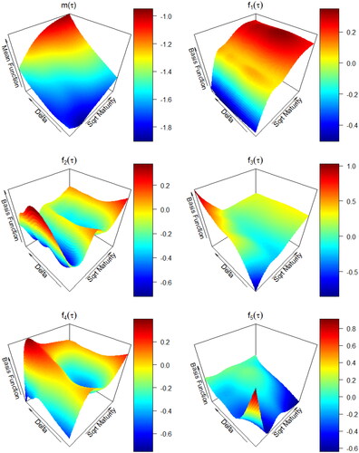
The mean function $m(\tau )$ demonstrates the characteristic “volatility skew” endemic to equity option markets. The Black-Scholes model assumes a Gaussian distribution for market returns. If such an assumption were true, the observed volatility surface would be flat. However, we see that the S&P500 returns exhibit both heavy tails and a negative skewness, leading to convexity and skewness in the mean function, respectively.

We have found that setting K = 5 leads to interpretable basis functions corresponding to local effects acting on specific regions of the domain. The first principal component $f_1(\tau )$ is negative when time to maturity is small while positive when time to maturity is large, resulting in a tilt of the surface with respect to maturity. The second principal component $f_2(\tau )$ results in a bending effect with respect to maturity. The third principal component $f_3(\tau )$ tilts the short maturity end of the surface with respect to delta. The fourth principal component $f_4(\tau )$ has a similar bending effect as the second but pushes the edges upward in general. The fifth principal component $f_5(\tau )$ pushes up one of the corners.

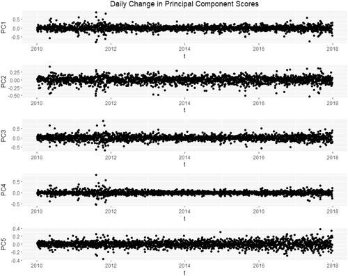
In an exploratory analysis, we see evidence for stochastic volatility. For five fixed sample domain points ${\tau }_1,\dots ,{\tau }_5,$ the differenced time courses ${\{Y_{t+1}({\tau }_j)-Y_t({\tau }_j)\}}_{t=1}^{T-1}$ are shown in Figure 2. The time-differenced principal component scores are shown in Figure 3. Both sets of series exhibit stochastic volatility and motivate the application of the FSV model. Because the amount of stochastic volatility observed in the previous section varies year-by-year, the model is fit separately to each of the 8 years of data.

Figure 2. Differenced time courses ${\{Y_{t+1}({\tau }_j)-Y_t({\tau }_j)\}}_{t=1}^{T-1}$ for five sample locations ${\tau }_1,\dots ,{\tau }_5,$ which exhibit stochastic volatility.

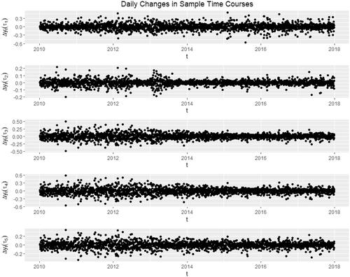
Figure 3. Differenced Principal Component Scores ${\beta }_{t+1,k}-{\beta }_{tk},$ which exhibit stochastic volatility.

4.4. Value-at-Risk Estimation for Option Portfolios

A forecast distribution for portfolio loss is required to estimate quantiles and thus Value-at-Risk. This section describes how to use the posterior samples ${\left\{{\mathit{\theta }}^j\right\}}_{j=1}^J$ produced by our MCMC algorithm to build a conditional forecast distribution ${\left\{L_{t+1}^{*j}\right\}}_{j=1}^J$ for a next-day option portfolio loss random variable $L_{t+1}={\Pi }_t(Y_{t+1})$ where ${\Pi }_t:L^2(\mathcal{T})\to \mathbb{R}.$ The option portfolio pricing functional Π_t is explicitly described by Equations 11–15. The forecast distribution ${\left\{{\mathit{\theta }}^j\right\}}_{j=1}^J$ is constructed from Equations 4.4(4) $${\mathit{h}}_t=\mathit{\mu }+{\mathit{\varphi }}^{\top }({\mathit{h}}_{t-1}-\mathit{\mu })+{\mathit{\zeta }}_t,{\mathit{\zeta }}_t\sim N_K\left[\mathbf{0},\text{diag}\left({\mathit{\sigma }}_{\zeta }^2\right)\right],$$(4) –14. The key quantity of interest in financial risk management is the Value-at-Risk (VaR) which is defined by the quantile of a loss distribution for a given time horizon and is defined in Equation 7(7) $$\text{VaR}(L_{t+1},1-\alpha )=\sup \left\{x\in \mathbb{R}:\mathbb{P}\left(L_{t+1}\le x\right)<1-\alpha \right\}$$(7) .

For this application, we complete the prior specification as follows. For each k, $$\begin{array}{c}{\mu }_k\sim N(0,1),\\ ({\varphi }_k+1)/2\sim \text{Beta}(20,1.5),\\ {\sigma }_k^2\sim {\chi }_1^2,\end{array}$$ while $$\begin{array}{c}\mathbf{\Psi }\sim {\text{Matrix}\mathrm{ }\text{Normal}}_{K,K}\left({\mathbf{0}}_K,{10}^6·{\mathit{I}}_K,{\mathit{I}}_K\right),\\ {\sigma }_{\epsilon }^2\sim \text{InvGamma}(0.001,0.001).\end{array}$$

The prior for ${\varphi }_k$ follows the example of Kim et al. (1998) and implies a prior mean of 0.86 to reflect the volatility clustering endemic to financial time series. We have found that the results are not sensitive to the choice of priors for μ_k and σ_k provided the series has a reasonable length. The hyperparameters of the matrix normal prior for $\mathbf{\Psi }$ and the inverse gamma prior for ${\sigma }_{\epsilon }^2$ were chosen so that these prior distributions do not strongly influence the results.

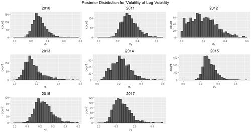
As we saw in our exploratory analysis (see Figures 2 and 3), the amount of stochastic volatility varies for each year. Thus, we fit the FSV model separately to each year of data. Figure 4 presents the 95% pointwise credible intervals for each of the log-volatility processes h_tk against t. Years 2010–2011 and 2015–2017 exhibit a higher degree of roughness in the random variation, indicating a higher presence of stochastic volatility for these years. This is further illustrated by the posterior histograms of the stochastic volatility parameter σ₁ appearing in Figure 5. The histograms are bounded away from zero, especially in the years 2010–2011 and 2015–2017. The results are similar for ${\sigma }_2,\dots ,{\sigma }_K.$

Figure 4. 95% pointwise credible bands for the latent log-volatility process with posterior median in bold. Dates range from start of 2010 to end of 2017. The roughness of random variation in h_tk indicates a notable presence of stochastic volatility in years 2010–2011 and 2015–2017.

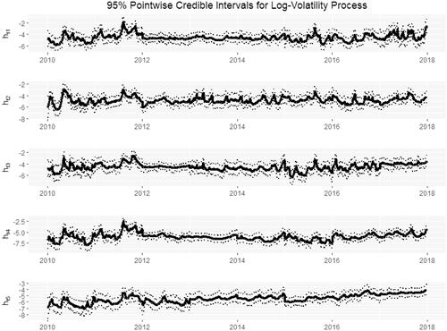
Figure 5. Posterior distributions for σ₁, the volatility of $h_{t1}.$ The histograms exhibit most of their probability mass away from 0 particularly in the years 2010–2011 and 2015–2017, indicating the presence of stochastic volatility.

To simplify the presentation of what follows, it should be understood that a posterior draw corresponds to the fit from the year containing t. For each posterior sample from the associated year’s model parameters ${\mathit{\theta }}^j=({\left\{{\mathit{\beta }}_t\right\}}^j,{\Psi }^j,{\sigma }_{\epsilon }^{2j},{\left\{{\mathit{h}}_t\right\}}^j,{\mathit{\mu }}^j,{\mathit{\varphi }}^j,{\mathit{\sigma }}^j),$ we forecast the option surface at time t + 1 from time t as follows: $$\begin{array}{c}{\mathit{\zeta }}_{t+1}^{*j}\sim N_K\left[0,\text{diag}\left({\mathit{\sigma }}^{2j}\right)\right]\\ {\mathit{h}}_{t+1}^{*j}={\mathit{\mu }}^j+{\mathit{\varphi }}^{j\top }({\mathit{h}}_t^j-{\mathit{\mu }}^j)+{\mathit{\zeta }}_{t+1}^{*j}\\ {\mathit{u}}_{t+1}^{*j}\mid {\mathit{h}}_{t+1}^{*j}\sim N_K\left[\mathbf{0},\text{diag}\left(e^{{\mathit{h}}_{t+1}^{*j}}\right)\right]\\ {\mathit{\beta }}_{t+1}^{*j}={\mathbf{\Psi }}^j{\mathit{\beta }}_t^j+{\mathit{u}}_{t+1}^{*j}\\ Y_{t+1}^{*j}(\tau )=F{(\tau )}^T{\mathit{\beta }}_{t+1}^{*j}\end{array}$$ where $F(\tau )={[f_1(\tau ),\dots ,f_K(\tau )]}^{\top }.$

Given this forecast of the implied volatility surface $Y_{t+1}^{*j}(\tau )$ and observation points ${\left\{{\tau }_{t+1|t,i}\right\}}_{i=1}^{n_t},$ we can compute the Black-Scholes log-implied volatilities ${\left\{y_{t+1,i}^{*j}\right\}}_{i=1}^{n_t}$ as (9) $$y_{t+1,i}^{*j}=m({\tau }_{t+1|t,i})+Y_{t+1}^{*j}({\tau }_{t+1|t,i})+{\epsilon }_{t+1,i}^{*j},{\epsilon }_{t+1,i}^{*j}\stackrel{\text{iid}}{\sim }N(0,{\sigma }_{\epsilon }^{j2}).$$(9) With their implied volatilities known, the options in the portfolio can be priced with the Black-Scholes formula (Black and Scholes 1973). If an option’s log-implied volatility at time t is y_t, then its price is given by (10) $$\text{Prem}\left[M_t,S_t,\kappa ,CP,r_t(M_t),q_t,y_t\right]=$$(10) (11) $$CP\left[S_t{e}^{-q_t{M}_t}\Phi (CP\times d_{+})-\kappa e^{-r_t(M_t)M_t}\Phi (CP\times d_{-})\right]$$(11) where (12) $$d_{\pm }=\frac{\hspace{0.17em}\log \hspace{0.17em}(S_t/\kappa )+\left[r_t(M_t)-q_t\pm \frac{1}{2}{e}^{2y_t}\right]M_t}{e^{y_t}\sqrt{M_t}}$$(12) and

• $M_t\equiv M_t({\tau }^1)={({\tau }^1)}^2/365$ is the time to maturity in years at time t,

• S_t is the spot price of S&P500 at time t,

• κ is the option strike price,

• $CP=\{\begin{array}{c}\mathrm{ }1\mathrm{ }\text{for}\text{ a }\text{call}\mathrm{ }\text{option},\mathrm{ }\hfill \\ -1\mathrm{ }\text{for}\text{ a }\text{put}\mathrm{ }\text{option},\hfill \end{array}$

• $r_t(M)$ is the risk-free rate at time t associated with time to maturity M,

• q_t is the dividend yield of S&P500 at time t,

• y_t is the log of implied volatility at time t,

• $\Phi$ is the standard normal cumulative distribution function,

and the Black–Scholes call option delta ${\tau }^2$ is computed from the above inputs as (13) $${\tau }^2=e^{-q_t{M}_t}\Phi (d_{+}).$$(13)

Suppose on day t the set of traded options are at locations ${\left\{{\tau }_{t,i}\right\}}_{i=1}^{n_t}.$ Then the updated observation points ${\left\{{\tau }_{t+1|t,i}\right\}}_{i=1}^{n_t}$ on day t + 1 are calculated as follows:

1. Days to maturity ${\tau }_{t+1|t,i}^1$ is reduced by the number of trading days between time t and t + 1. This is usually one day but can be more because of weekends and holidays.

2. Option delta ${\tau }_{t+1|t,i}^2$ is assumed equal to the previous day’s value ${\tau }_{t,i}^2.$

3. The other option parameters $S_{t+1|t},\kappa ,r_{t+1|t}(M_{t+1}),q_{t+1|t}$ are held equal to day t’s values $S_t,\kappa ,r_t(M_t),q_t$ to prevent looking ahead to future data.

Thus, for each posterior sample ${\left\{y_{t+1,i}^{*j}\right\}}_{i=1}^{n_t},$ we can produce joint forecasts for the option prices ${\left\{F{P}_{t+1,i}^{*j}\right\}}_{i=1}^{n_t}$ where $$F{P}_{t+1,i}^{*j}=\text{Prem}\left[M_{t+1},S_t,\kappa ,CP,r_t(M_t),q_t,y_{t+1,i}^{*j}\right].$$

These forecasted option prices can be compared to the actual option prices ${\left\{A{P}_{t,i}\right\}}_{i=1}^{n_t}$ and ${\left\{A{P}_{t+1,i}\right\}}_{i=1}^{n_t}$ on days t and t + 1, respectively, to assess the performance of the forecast. Given a portfolio with c_ti units of option i for $i=1,\dots ,n_t,$ we can compute the forecasted loss distribution ${\left\{L_{t+1}^{*j}\right\}}_{j=1}^J$ and actual loss $L_{t+1}$ of the portfolio as (14) $$L_{t+1}^{*j}=\sum _{i=1}^{n_t}{c}_{ti}\left(A{P}_{t,i}-F{P}_{t+1,i}^{*j}\right)$$(14) (15) $$L_{t+1}=\sum _{i=1}^{n_t}{c}_{ti}\left(A{P}_{t,i}-A{P}_{t+1,i}\right).$$(15) We can take sample quantile of the forecasted loss distribution as our estimate of the $(1-\alpha )100\%$ one-day Value-at-Risk, setting (16) $$\widehat{\text{VaR}}(L_{t+1},1-\alpha )=\text{quantile}\left({\left\{L_{t+1}^{*j}\right\}}_{j=1}^J,1-\alpha \right).$$(16) The next step is to assess whether the quantiles of the forecast distribution match the quantiles of the true loss distribution.

4.5. Backtesting Value-at-Risk

In order to evaluate the accuracy of our Value-at-Risk estimates, we can test if the historically observed exceedence rates of our quantile estimates are consistent with the true quantile levels. This process of evaluation based on historical data is known as backtesting. A 95% Value-at-Risk estimate should be breached by approximately 5% of observed losses if the observed trials are independent and the estimate is accurate. We can test whether the estimator proposed in Subsection 4.4 is accurate in this sense using the binomial hypothesis test discussed in Subsection 4.1.

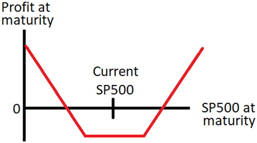
We focus on option portfolios whose values are most sensitive to movements in volatility. An option strangle is a portfolio consisting of an out-of-money call option (whose strike is below the current S&P 500 level) and an out-of-money put option (whose strike is above the current S&P 500 level) where the call and put strikes are roughly the same distance apart from the current S&P 500 level. Such portfolios are particularly sensitive to movements in implied volatility $e^{Y_t(\tau )},$ since a strangle profits from large moves in the S&P but loses money on small moves. The profit diagram of a strangle portfolio is illustrated in Figure 6.

Figure 6. Profit diagram for an option strangle portfolio.

The binomial test of Kupiec (1995) described in Subsection 4.1 requires independent trials, so we use a different randomized option portfolio on each trading day in order to decorrelate the trials. To construct these randomized portfolios, on each day $t=1,\dots ,T-1,$ a set of random out-of-money options are chosen from the subset of options common to both days t and t + 1 so that the actual price movement can be computed. These out-of-money options are chosen in 25 unique pairs of calls and puts so that we can form strangle positions. Hence, if a call option with strike price ${\kappa }_1>S_t$ is selected, then the put option whose strike is closest to ${\kappa }_2=S_t-({\kappa }_1-S_t)$ is also chosen so that the put and call options are roughly the same distance apart from the current spot price with both options out-of-money.

For each $t=1,\dots ,2012,$ consider a simple randomized portfolio ${\left\{c_{ti}\right\}}_{i=1}^{50}$ on these 50 options where each c_ti is either 1 or −1 with equal probability. These coefficients determine the portfolio pricing functionals $\left\{{\Pi }_t\right\}$ through Equations 14(14) $$L_{t+1}^{*j}=\sum _{i=1}^{n_t}{c}_{ti}\left(A{P}_{t,i}-F{P}_{t+1,i}^{*j}\right)$$(14) and 15(15) $$L_{t+1}=\sum _{i=1}^{n_t}{c}_{ti}\left(A{P}_{t,i}-A{P}_{t+1,i}\right).$$(15) . Since the actual price movements of these portfolios are known, we can apply the binomial hypothesis test described in Subsection 4.1 to the one-day Value-at-Risk estimator in Equation 16(16) $$\widehat{\text{VaR}}(L_{t+1},1-\alpha )=\text{quantile}\left({\left\{L_{t+1}^{*j}\right\}}_{j=1}^J,1-\alpha \right).$$(16) . A separate binomial test is done for each year. The 95% confidence intervals of the exceedence rates of VaR95, VaR97.5, and VaR99 are shown in blue in Figure 7.

Figure 7. 95% confidence intervals for the exceedence rates of value-at-risk. CV indicates constant volatility while SV indicates stochastic volatility.

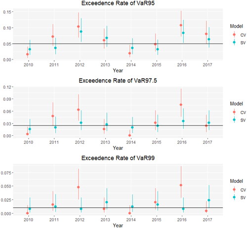
For comparison, we also made forecasts based on a benchmark model with constant volatility. The benchmark model assumes each coefficient series ${\left\{{\beta }_{tk}\right\}}_{t=1}^T$ has constant volatility $v_k.$ Setting $\mathit{v}={(v_1,\dots ,v_K)}^{\top },$ the benchmark model satisfies $$\begin{array}{cc}{\mathit{y}}_t={\mathit{m}}_t+{\mathit{F}}_t{\mathit{\beta }}_t+{\mathit{\epsilon }}_t,& {\mathit{\epsilon }}_t\sim N_{n_t}\left(\mathbf{0},{\sigma }_{\epsilon }^2\mathit{I}\right),\\ {\mathit{\beta }}_t=\mathbf{\Psi }{\mathit{\beta }}_{t-1}+{\mathit{\gamma }}_t,& {\mathit{\gamma }}_t\sim N_K\left[\mathbf{0},\text{diag}(\mathit{v})\right]\end{array}$$ for all t. Each v_k is assigned an independent $\text{InvGamma}(a_k,b_k)$ prior. The full conditional distribution for v is standard, and all other full conditional distributions remain the same with the substitution ${\mathit{h}}_t=\hspace{0.17em}\log \hspace{0.17em}(\mathit{v})$ for each t.

The results in Figure 7 indicate that the exceedence rates of the stochastic volatility-based VaR estimates are generally closer to the true quantile levels than those of the constant volatility-based VaR estimates. The binomial confidence intervals associated with the stochastic volatility model’s VaR estimates include the true level in almost all years, while the intervals associated with the constant volatility model’s VaR estimates miss far more frequently. These findings indicate that incorporating stochastic volatility leads to better quantile estimates.

5. Conclusion

To review, we introduced an analogue of the familiar stochastic volatility model for functional time series, with the goal of accurately modeling option surfaces. We reduced that functional specification to a finite dimensional vector time series model and discussed a strategy for Bayesian inference that enables forecasting, quantile estimation, and other uncertainty quantification. Motivated by an exploratory analysis that revealed evidence of stochastic volatility, we applied the FSV model to SPX option surfaces and demonstrated through backtesting that the FSV model leads to improved quantile estimates and thus improved Value-at-Risk estimates for option portfolios.

Additional information

Funding

The authors gratefully acknowledge financial support from National Science Foundation Awards 2114143, 1934985, 1940124, and 1940276.

References

- Asai M, McAleer M, Yu J. 2006. Multivariate stochastic volatility: review. Econom Rev. 25(2–3):145–175.
- Aue A, Horváth LF, Pellatt D. 2017. Functional generalized autoregressive conditional heteroskedasticity. J Time Ser Anal. 38(1):3–21.
- Aue A, Klepsch J. 2017. Estimating functional time series by moving average model fitting. arXiv:170100770.
- Aue A, Norinho DD, Hörmann S. 2015. On the prediction of stationary functional time series. J Am Stat Assoc. 110(509):378–392.
- Besse PC, Cardot H, Stephenson DB. 2000. Autoregressive forecasting of some functional climatic variations. Scand J Stat. 27(4):673–687.
- Black F, Scholes M. 1973. The pricing of options and corporate liabilities. J Polit Econ. 81(3):637–654.
- Bollerslev T. 1986. Generalized autoregressive conditional heteroskedasticity. J Econom. 31(3):307–327.
- Bollerslev T. 1990. Modelling the coherence in short-run nominal exchange rates: a multivariate generalized ARCH model. Rev Econom Stat. 72(3):498–505.
- Bollerslev T, Engle R, Wooldridge J. 1988. A capital asset pricing model with time-varying covariances. J Polit Econ. 96(1):116–131.
- Bosq D. 2000. Linear processes in function spaces: theory and applications. Lecture notes in statistics. New York: Springer.
- Bosq D. 2014. Computing the best linear predictor in a Hilbert space. applications to general ARMAH processes. J Multivariate Anal. 124:436–450.
- Brillinger DR. 1981. Time series: data analysis and theory. Vol. 36. Philadelphia (PA): SIAM.
- Chakraborty A, Panaretos VM. 2019. Testing for the rank of a covariance operator. The annals of statistics (forthcoming). https://arxiv.org/pdf/1901.02333.pdf.
- Chan JC. 2021. Minnesota-type adaptive hierarchical priors for large Bayesian VARs. Int J Forecasting. 37(3):1212–1226.
- Chen Y, Li B. 2017. An adaptive functional autoregressive forecast model to predict electricity price curves. J Business Econ Stat. 35(3):371–388.
- Cressie N, Wikle C. 2015. Statistics for spatio-temporal data. New York: Wiley.
- Daniélsson J. 1998. Multivariate stochastic volatility models: estimation and a comparison with VGARCH models. J Empirical Finance. 5(2):155–173.
- Doan T, Litterman R, Sims C. 1984. Forecasting and conditional projection using realistic prior distributions. Econom Rev. 3(1):1–100.
- Engle RF. 1982. Autoregressive conditional heteroscedasticity with estimates of the variance of United Kingdom inflation. Econometrica. 50(4):987–1007.
- Gatheral J. 2006. The volatility surface: a practitioner’s guide. Wiley finance series. New York: John Wiley & Sons.
- Gelman A, Carlin J, Stern H, Dunson D, Vehtari A, Rubin D. 2013. Bayesian data analysis. 3rd ed. Chapman & Hall/CRC Texts in statistical science. Boca Raton (FL): Taylor & Francis.
- Ghysels E, Harvey A, Renault E. 1996. Stochastic volatility. Montreal: Centre Interuniversitaire de Recherche en Économie Quantitative, CIREQ. Cahiers de recherche.
- Giannone D, Lenza M, Primiceri GE. 2015. Prior selection for vector autoregressions. Rev Econ Stat. 97(2):436–451.
- Hall P, Vial C. 2006. Assessing the finite dimensionality of functional data. J R Stat Soc B. 68(4):689–705.
- Han CH, Liu WH, Chen TY. 2014. VaR/CVaR estimation under stochastic volatility models. Int J Theor Appl Finan. 17(02):1450009.
- Harvey A, Ruiz E, Shephard N. 1994. Multivariate stochastic variance models. Rev Econ Stud. 61(2):247–264.
- Heston SL. 1993. A closed-form solution for options with stochastic volatility with applications to bond and currency options. Rev Finance Stud. 6(2):327–343.
- Heston SL, Nandi S. 2000. A closed-form GARCH option valuation model. Rev Finance Stud. 13(3):585–625.
- Hörmann S, Horváth L, Reeder R. 2013. A functional version of the ARCH model. Econom Theory. 29(2):267–288.
- Hörmann S, Kidziński L, Hallin M. 2015. Dynamic functional principal components. J R Stat Soc B. 77(2):319–348.
- Hörmann S, Kokoszka P. 2010. Weakly dependent functional data. Ann Stat. 38(3):1845–1884.
- Horváth L, Kokoszka P. 2012. Inference for functional data with applications. Springer series in statistics. New York: Springer.
- Hsing T, Eubank R. 2015. Theoretical foundations of functional data analysis, with an introduction to linear operators. Wiley series in probability and statistics. Chichester: Wiley.
- Huang AY. 2015. Value at risk estimation by threshold stochastic volatility model. Appl Econ. 47(45):4884–4900.
- Huang SF, Guo M, Chen MR. 2020. Stock market trend prediction using a functional time series approach. Quant Finance. 20(1):69–79.
- Hull J. 2018. Options, futures, and other derivatives. London: Pearson.
- Hull J, White A. 1987. The pricing of options on assets with stochastic volatilities. J Finance. 42(2):281–300.
- Hyndman R, Booth H. 2008. Stochastic population forecasts using functional data models for mortality, fertility and migration. Int J Forecasting. 24(3):323–342.
- Hyndman RJ, Shahid Ullah M. 2007. Robust Forecasting of mortality and fertility rates: a functional data approach. Comput Stat Data Anal. 51(10):4942–4956.
- Hyndman RJ, Booth H, Yasmeen F. 2013. Coherent mortality forecasting: the product-ratio method with functional time series models. Demography. 50(1):261–283.
- Jang PA, Matteson DS. 2018. Spatial correlation in weather forecast accuracy: a functional time series approach. JSM 2018 Proceedings, Statistical Computing Section, 2776–2784.
- Karhunen K. 1947. Über lineare Methoden in der Wahrscheinlichkeitsrechnung. Annales Academiae Scientiarum Fennicae. 37:1–79.
- Kastner G. 2016. Dealing with stochastic volatility in time series using the R package stochvol. J Stat Software Art. 69(5):1–30.
- Kastner G, Frühwirth-Schnatter S. 2014. Ancillarity-sufficiency interweaving strategy (ASIS) for boosting MCMC estimation of stochastic volatility models. Comput Stat Data Anal. 76:408–423. CFEnetwork: the annals of computational and financial econometrics.
- Kim S, Shepherd N, Chib S. 1998. Stochastic volatility: likelihood inference and comparison with ARCH models. Rev Econ Stud. 65(3):361–393.
- King MC, Staicu AM, Davis JM, Reich BJ, Eder B. 2018. A functional data analysis of spatiotemporal trends and variation in fine particulate matter. Atmos Environ. 184:233–243.
- Klepsch J, Klüppelberg C, Wei T. 2017. Prediction of functional ARMA processes with an application to traffic data. Econom Stat. 1(C):128–149.
- Kneip A. 1994. Nonparametric estimation of common regressors for similar curve data. Ann Statist. 22(3):1386– 1427.
- Kowal DR, Matteson DS, Ruppert D. 2017. A Bayesian multivariate functional dynamic linear model. J Am Stat Assoc. 112(518):733–744.
- Kowal DR, Matteson DS, Ruppert D. 2019. Functional autoregression for sparsely sampled data. J Business Econ Stat. 37(1):97–109.
- Kupiec PH. 1995. Techniques for verifying the accuracy of risk measurement models. JOD. 3(2):73–84.
- Li D, Robinson PM, Shang HL. 2020. Long-range dependent curve time series. J Am Stat Assoc. 115(530):957–971.
- Litterman RB. 1986. Forecasting with Bayesian vector autoregressions – five years of experience. J Business Econ Stat. 4(1):25–38.
- Loève M. 1945. Fonctions Aléatoires de Second Ordre. Comptes Rendus de l’Académie des Sciences. Série I: Mathématique. 220:469.
- Mohammadi N, Panaretos VM. 2021. Detecting whether a stochastic process is finitely expressed in a basis. https://arxiv.org/abs/2111.01542
- OptionMetrics. 2017. IvyDB US file and data reference manual, version 3.1, Rev. 1/17/2017. New York (NY): OptionMetrics; p. 10019.
- Quang P, Klein T, Nguyen N, Walther T. 2018. Value-at-risk for south-east Asian stock markets: stochastic volatility vs. GARCH. JRFM. 11(2):18.
- Ramsay J, Ramsay J, Silverman B, Media SS, Silverman H. 2005. Functional data analysis. Springer series in statistics. Cham: Springer.
- Robert CP, Casella G. 2004. Monte Carlo statistical methods. Springer texts in statistics. Cham: Springer.
- Ruiz-Medina M, Espejo R, Ugarte M, Militino A. 2014. Functional time series analysis of spatio–temporal epidemiological data. Stoch Environ Res Risk Assess. 28(4):943–954.
- Sadorsky P. 2005. Stochastic volatility forecasting and risk management. Appl Financ Econ. 15(2):121–135.
- Sen R, Klüppelberg C. 2019. Time series of functional data with application to yield curves. Appl Stochastic Models Bus Ind. 35(4):1028–1043.
- Shang HL. 2013. Functional time series approach for forecasting very short-term electricity demand. Appl Stat. 40(1):152–168.
- Shang HL, Booth H, Hyndman R. 2011. Point and interval forecasts of mortality rates and life expectancy: a comparison of ten principal component methods. DemRes. 25:173–214.
- Shephard N. 1996. Statistical aspects of ARCH and stochastic volatility. London: Chapman & Hall; p. 1–67. Reprinted in the Survey of Applied and Industrial Mathematics, Issue on Financial and Insurance Mathematics, 3, 764–826, Scientific Publisher TVP, Moscow, 1996 (in Russian).
- Shephard N, Andersen TG. 2009. Stochastic volatility: origins and overview. Berlin, Heidelberg: Springer Berlin Heidelberg. p. 233–254.
- Taylor S. 1982. Financial returns modelled by the product of two stochastic processes-a study of the daily sugar prices 1961-75. Time Ser Anal Theory Pract. 1:203–226.
- Taylor S. 1986. Modelling financial time series. New York: Wiley.
- Taylor S. 1994. Modelling stochastic volatility: a review and comparative study. Math Finance. 4(2):183–204.
- Vrontos ID, Dellaportas P, Politis DN. 2003. A full-factor multivariate GARCH model. Econom J. 6(2):312–334.
- Wood SN. 2011. Fast stable restricted maximum likelihood and marginal likelihood estimation of semiparametric generalized linear models. J R Stat Soc B. 73(1):3–36.
- Yasmeen F, Sharif M. 2015. Functional time series (FTS) forecasting of electricity consumption in Pakistan. IJCA. 124(7):15–19.
- Yu J, Meyer R. 2006. Multivariate stochastic volatility models: Bayesian estimation and model comparison. Econom Rev. 25(2–3):361–384.