Model Selection for Exposure-Mediator Interaction

Abstract

In mediation analysis, the exposure often influences the mediating effect, i.e., there is an interaction between exposure and mediator on the dependent variable. When the mediator is high-dimensional, it is necessary to identify non-zero mediators ($M$) and exposure-by-mediator ($X$-by-$M$) interactions. Although several high-dimensional mediation methods can naturally handle $X$-by-$M$ interactions, research is scarce in preserving the underlying hierarchical structure between the main effects and the interactions. To fill the knowledge gap, we develop the XMInt procedure to select $M$ and $X$-by-$M$ interactions in the high-dimensional mediators setting while preserving the hierarchical structure. Our proposed method employs a sequential regularization-based forward-selection approach to identify the mediators and their hierarchically preserved interaction with exposure. Our numerical experiments showed promising selection results. Furthermore, we applied our method to ADNI morphological data and examined the role of cortical thickness and subcortical volumes on the effect of amyloid-beta accumulation on cognitive performance, which could be helpful in understanding the brain compensation mechanism.

Keywords:

• Brain compensation
• exposure-by-mediator interaction
• hierarchical structure
• high-dimensional mediators
• model selection
• mediation analysis
• neuroimaging

1. Introduction

A mediation model examines how an independent variable or an exposure ($X$) affects a dependent variable ($Y$) through one or more intervening variables or mediators ($M$) (Baron and Kenny 1986; Daniel et al. 2015; Holland 1988; Imai et al. 2010; Imai and Yamamoto 2013; MacKinnon 2008; Pearl 2013; Preacher and Hayes 2008; Robins and Greenland 1992; Sobel 2008; VanderWeele T 2015; VanderWeele T and Vansteelandt 2014; VanderWeele TJ 2011). 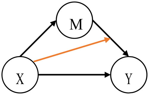In the mediation mechanism, we often observe that $X$ influences the mediating effect of $M$ on $Y$, i.e., there is an interaction between $X$ and $M$ on the dependent variable ($Y$), as represented in Figure 1.

Figure 1. A graphical representation of the mediation effect of the intervening variable $M$ on the relationship between the independent variable $X$ and the dependent variable $Y$ (black arrows, upper triangular part) and the interaction effect between $X$ and $M$ (orange arrow).

A typical multivariate mediation model with exposure-by-mediator interactions takes the following form in (1). In a general context, let $X$ represent the independent variable or the exposure of interest, let $Y$ represent the dependent variable or the outcome of interest, let $M_v,$ where $v=1,\dots ,V,$ represent $V$ potential mediator variables ($M$), and let $X\times M_v$ represent the interaction term between the exposure variable $X$ and the potential mediator variable $M_v.$ Denote $\mathbf{x}={\left(x_1\cdots x_N\right)}^{\top }$ as the $N\times 1$ vector of observed exposure measurements from $N$ subjects, $\mathbf{y}={\left(y_1\cdots y_N\right)}^{\top }$ as the $N\times 1$ vector of observed outcome responses from $N$ subjects, and ${\mathbf{M}}_{N\times V}={\left(m_{i,v}\right)}_{\begin{array}{c}i=1,\dots ,N;\\ v=1,\dots ,V\end{array}}={\left({\mathbf{m}}_1^{\top }\cdots {\mathbf{m}}_N^{\top }\right)}^{\top }$ as the $N\times V$ matrix of $V$ observed potential mediator variables from $N$ subjects. For each subject $i=1,\dots ,N,$ (1) $$\genfrac{}{}{0pt}{}{{\mathbf{m}}_i={\mathit{a}}_0+\mathit{a}{x}_i+{{\mathit{e}}_1}_i\mathrm{ }\left(\mathit{\text{path}}-a\mathrm{ }\mathit{\text{model}}\right),}{y_i=c_0+c{x}_i+{\mathbf{m}}_i^{\mathrm{\top }}{\mathit{b}}_1+\left(x_i\times {\mathbf{m}}_i^{\mathrm{\top }}\right){\mathit{b}}_2+{e_2}_i\mathrm{ }\left(\mathit{\text{path}}-b\mathrm{ }\mathit{\text{model}}\right),}$$(1) where ${\mathbf{m}}_i={\left(m_{i,1}···m_{i,V}\right)}^{\mathrm{\top }},$ $x_i\times {\mathbf{m}}_i^{\mathrm{\top }}=\left({x_{i}m}_{i,1}···{x_{i}m}_{i,V}\right),{\mathit{a}}_0={\left({a_0}_1···{a_0}_V\right)}^{\mathrm{\top }},$ $\mathit{a}={\left(a_1···a_V\right)}^{\mathrm{\top }},$ ${{\mathit{e}}_1}_i={\left({e_1}_{i,1}···{e_1}_{i,V}\right)}^{\mathrm{\top }}\sim \mathit{\text{MVN}}(0,\mathbf{\Sigma }),$ ${\mathit{b}}_1={\left({b_1}_1···{b_1}_V\right)}^{\mathrm{\top }},$ ${\mathit{b}}_2={\left({b_2}_1···{b_2}_V\right)}^{\mathrm{\top }},$ and ${e_2}_i\sim N(0,{\sigma }^2).$ Subjects are assumed to be independent and identically distributed (i.i.d.). Any $M_v$ with non-zero $a_v$ and ${b_1}_v$ coefficients is considered to be a mediator. Any $X\times M_v$ with non-zero ${b_2}_v$ coefficient is considered to have an interaction effect.

In the single mediator case, T. J. VanderWeele (2014) proposed the four-way decomposition method to handle the $X$-by-$M$ interaction, which united methods that attribute effects to interactions and methods that assess mediation and was used in literature (e.g., Wang Y et al. 2019) to understand the mediated interaction effect. This decomposition idea was later extended to the few mediators case, such as in Bellavia and Valeri (2018).

New mediation methods have also been developed to address the issue of high dimensions in the mediators. Some used regularization-based methods (Li et al. 2021; Serang et al. 2017; Zhao Y and Luo 2016). Others used hybrid methods such as the combined filter method with coordinate descent algorithm (van Kesteren and Oberski 2019), screening and regularization (Luo et al. 2020; Schaid and Sinnwell 2020; Zhang et al. 2016, 2021), and dimension reduction and regularization (Zhao Y et al. 2020).

Nevertheless, for models involving interactions with high-dimensional data, it is important to preserve the underlying hierarchical structure between the main effects and the interactions, because models with interactions but without corresponding marginal effects can be difficult to interpret in practice (Chipman 1996; Choi et al. 2010; Hao and Zhang 2017; Nelder 1977; Yuan et al. 2009; Zhao P et al. 2009). This remains the case in the mediation model with high-dimensional mediators. In regression settings, maintaining the hierarchical structure between the main effects and the interactions requires that the interaction terms are only allowed to be included in the model if the corresponding main effects are also present in the model (Bien et al. 2013; Hao et al. 2018; Zhao P et al. 2009). Take as an example the model with interactions formulated as $Y={\gamma }_0+{\gamma }_1{X}_1+\cdots +{\gamma }_p{X}_p+{\gamma }_{1,2}{X}_1{X}_2+\cdots +{\gamma }_{p,p}{X}_p^2+\epsilon ,$ where $\epsilon \sim N(0,{\sigma }_0^2),$ the hierarchical structure is considered preserved if for any $X_i{X}_j$ term that has a non-zero coefficient, its consisting variables $X_i$ and $X_j$ also have non-zero coefficients. Such concept is also referred as “heredity”, “marginality principle”, and being “hierarchically well-formulated” in previous literature, such as in Hamada and Wu (1992), Chipman (1996), Nelder (1977), and Peixoto (1987) (Bien et al. 2013). Similarly, in the mediation settings as in (1), we consider the hierarchical structure between the main effects and interactions to be preserved if whenever there is an interaction effect between the exposure $X$ and $M_v,$ the corresponding $M_v$ has to be a mediator; in other words, whenever the coefficient for $X\times M_v$ is non-zero, the corresponding $M_v$ should also have non-zero $a_v$ and ${b_1}_v$ coefficients.

To address the issue of hierarchical structure, in regression settings, regularization methods with different penalty functions (Bien et al. 2013; Choi et al. 2010; Yuan et al. 2009; Zhao P et al. 2009) have been developed to aid the interaction selection, but they become infeasible as the number of independent variables increases (Hao et al. 2018). To address such limitation, Hao et al. (2018) proposed an efficient interaction selection method for high-dimensional data, the regularization algorithm under marginality principle (RAMP), in which possible interaction terms are sequentially added based on the current main effects.

Compared to the regression settings, it is more challenging to preserve the hierarchical structure between the main effects and interactions in the mediation analysis because model selection now involves two models: $M$ on $X$ and $Y$ on $M.$ Although the high-dimensional mediation methods mentioned earlier may naturally handle $X$-by-$M$ interactions, research is scarce in preserving such hierarchy. Therefore, in this paper, we aim to identify the mediators and the exposure-by-mediator interactions in the high-dimensional mediators setting while addressing the underlying hierarchical structure between the main effects and interactions.

This identification of mediators and their hierarchically preserved interaction with exposure can be useful in explaining how the brain reacts during the process of brain-related changes and in understanding the brain compensation mechanism, defined as the phenomenon that the effect of the brain on the outcome is altered. For example, under the context of cognitive aging and brain pathology, where we have cognitive or clinical performance as the outcome, aging or pathology as the exposure, and certain brain measures such as cortical thickness as the potential mediators, we often observe that thinner cortical thickness ($M$) is associated with the worse cognitive performance ($Y$), and further, in the presence of some pathology ($X$), we observe the opposite association or no association anymore. In other words, the brain acts differently on the outcome because of the exposure (i.e., there is $X$-by-$M$ interaction), which illustrates the brain compensation mechanism based on our definition. Or alternatively, we may think that the brain tries to compensate for the loss in cognition due to the pathology, which is also indicative of the idea of compensation.

Our proposed method employs a sequential regularization-based forward-selection approach to identify the mediators and their interactions with exposure while preserving the hierarchical structure between them. Specifically, we propose an adaptive forward-selection regularization strategy for the preservation of hierarchical structure. The main idea of the process is that while we generate a series of models through a sequence of decreasing tuning parameters (e.g., $K$ models from $K$ tuning parameters; we denote the generation of $k$-th model as the $k$-th step, where $k=1,\dots ,K$), for each tuning parameter (i.e., at each step) we impose penalization on a subset of coefficients based on the identified mediators and interactions from the model generated with the previous tuning parameter (i.e., from the previous step) to enforce the hierarchical structure, and finally the optimal model is determined as the one with the smallest Haughton’s Bayesian information criterion (HBIC) among all the generated models. The rule of this adaptive penalization is that, starting from a model with no mediators and no interactions (i.e., penalize all), if a mediator is identified but its corresponding interaction term is not, we will include the identified mediator in the next step (i.e., not penalize it); if both the mediator and its corresponding interaction are identified, we will include both in the next step (i.e., not penalize both); if an interaction is identified, but its involving $M$ is not, we will not only include the interaction but also include the involving $M$ in the next step (i.e., not penalize both) to preserve the hierarchical structure. Recently, C. Wang et al. (2020) proposed a method designed specifically for high-dimensional compositional microbiome mediators, in which the selection of the interaction between treatment and mediators was considered. In contrast to their method, our method focuses on the continuous mediators, which do not have any sum constraint on the mediators as in the microbiome data. In addition, instead of adding overall penalties to the objective function to preserve the hierarchical structure as in C. Wang et al. (2020), we adopt an adaptive way to update the penalties and include the potential mediator if either its interaction with the exposure is identified or its main effect is identified in the previous step.

In this paper, we first introduced our proposed algorithm in Section 2. Then, we presented the simulation results in Section 3. Finally, we applied our method to the real-world human brain imaging data and examined the role of cortical thickness and subcortical volumes on the relationship between amyloid beta accumulation and cognitive performance in Section 4.

2. Methods

We aim to identify the mediators ($M$) and their interactions with exposure ($X$) while preserving the hierarchical structure between the main effects and interaction effects. The multivariate mediation model that we consider takes the form in model (1), introduced in Section 1. Under the Gaussian assumption of the i.i.d. error terms, the log-likelihood is given as (2) $$\begin{array}{l}\mathcal{l}\left(\mathit{\theta }\right)=\sum _{i=1}^N{\mathcal{l}}_{y,\mathbf{m}|\mathit{\theta }}\left(\mathit{\theta }\right|y_i,{\mathbf{m}}_i)=\sum _{i=1}^N{\mathcal{l}}_{y|\mathbf{m},\mathit{\theta }}\left(\mathit{\theta }\right|y_i,{\mathbf{m}}_i)+\sum _{i=1}^N{\mathcal{l}}_{\mathbf{m}|\mathit{\theta }}\left(\mathit{\theta }\right|{\mathbf{m}}_i)\\ =-\frac{N}{2}\mathrm{\text{log}}\hspace{0.17em}\left(2\pi \right)-\frac{\mathit{\text{NV}}}{2}\mathrm{l}\mathrm{\text{og}}\left(2\pi \right)-\frac{N}{2}\mathrm{\text{log}}\hspace{0.17em}{\sigma }^2+\frac{N}{2}\mathrm{\text{log}}\hspace{0.17em}\left|\mathbf{\Omega }\right|-\frac{1}{2{\sigma }^2}\sum _{i=1}^N{\left(y_i-c_0-c{x}_i-{\mathbf{m}}_i^{\mathrm{\top }}{\mathit{b}}_1-\left(x_i\times {\mathbf{m}}_i^{\mathrm{\top }}\right){\mathit{b}}_2\right)}^2-\frac{1}{2}\sum _{i=1}^N{\left({\mathbf{m}}_i-{\mathit{a}}_0-\mathit{a}{x}_i\right)}^{\mathrm{\top }}\mathbf{\Omega }\left({\mathbf{m}}_i-{\mathit{a}}_0-\mathit{a}{x}_i\right),\end{array}$$(2) where $\mathbf{\Omega }={\mathbf{\Sigma }}^{-1}.$

We denote $\mathcal{M}=\{1,2,\dots ,V\}$ be the index set for all of the $V$ potential mediators, ${\mathcal{M}}_k$ be the index set for the mediators identified in step $k,$ where step $k$ was introduced in the introduction and refers to the generation of the $k$-th model using the corresponding $k$-th tuning parameter defined in details below in 1. Initialization, ${\mathcal{M}}_k^c=\mathcal{M}-{\mathcal{M}}_k$ be the index set for the remaining $M$ variables (out of $V$ variables), ${\mathcal{I}}_k$ be the index set for the involving $M$ variables in the interaction terms identified in step $k,$ and ${\mathcal{I}}_k^c=\mathcal{M}-{\mathcal{I}}_k$ be the index set for the involving $M$ variables in remaining interaction terms (out of $V$ variables).

Our algorithm is described as follows. Table 1 provides a summary of the algorithm.

1. Initialization

First, we standardize the data. Specifically, we standardize $\mathbf{x},\mathbf{y},$ and each column of $\mathbf{M},$ by subtracting its mean and dividing by its standard deviation, so that each variable has a mean of zero and a standard deviation of one. We will use the standardized data in our proposed algorithm.

Next, using the standardized data, we generate an exponentially decaying sequence, which will be served as regularization parameters for model tuning. Particularly, we compute ${\lambda }_{\mathrm{\text{max}}}=N^{-1}\mathrm{\text{max}}\hspace{0.17em}\left|{\left(\mathbf{x} \mathbf{M} \mathbf{x}\times \mathbf{M}\right)}^{\top }\mathbf{y}\right|$ and ${\lambda }_{\mathrm{\text{min}}}=\zeta {\lambda }_{\mathrm{\text{max}}}$ for some small $\zeta >0$ (e.g., 0.05), where ${\left(\mathbf{x} \mathbf{M} \mathbf{x}\times \mathbf{M}\right)}_{N\times (2V+1)}$ is the matrix that column-wisely combines ${\mathbf{x}}_{N\times 1},$ $\mathbf{M}{}_{N\times V},$ and ${\left(\mathbf{x}\times \mathbf{M}\right)}_{N\times V}={\left(x_1\times {\mathbf{m}}_1^{\mathrm{\top }}\cdots x_N\times {\mathbf{m}}_N^{\top }\right)}^{\top }.$ Based on the determined ${\lambda }_{\mathrm{\text{max}}}$ and ${\lambda }_{\mathrm{\text{min}}},$ we generate an exponentially decaying sequence with length $K$ (e.g., 20), ${\lambda }_{\mathrm{\text{max}}}={\lambda }_1>{\lambda }_2>···>{\lambda }_K={\lambda }_{\mathrm{\text{min}}}.$ Such generation process for tuning parameters is typical in linear regression literature (e.g., Friedman et al. 2010; Hao et al. 2018) and is modified particularly for our mediation model with interaction terms by additionally including $\mathbf{M}$ and $\mathbf{x}\times \mathbf{M}$ in the computation of ${\lambda }_{\mathrm{\text{max}}}.$ Also, we start with ${\mathcal{M}}_0=\varnothing$ and ${\mathcal{I}}_0=\varnothing .$ Note that $c_0=0$ and ${\mathit{a}}_0=0$ after the data standardization.

• 2. Find regularization path

For each $k=1,\dots ,K,$ we minimize the following objective function (3), in the form of twice negative log-likelihood (after removing constant terms that do not depend on parameters of interest) plus penalties, with respect to $c,\mathit{a},{\mathit{b}}_1,{\mathit{b}}_2,$ where ${\Vert {\mathbf{z}}_{p\times 1}\Vert }_1={\Vert {\left(z_1\cdots z_p\right)}^{\top }\Vert }_1$ is defined as ${\sum }_{i=1}^p\left|z_i\right|$ and the upper-diagonal elements of $\mathbf{\Omega }={\left(w_{\mathit{\text{gh}}}\right)}_{g,h=1,\dots ,V}$ is defined (in a vector form) as $\mathbf{w}=\left\{w_{g<h}\right\}={\left(w_{12} w_{13}\cdots w_{1V} w_{23} w_{24}\cdots w_{2V}\cdots w_{\left(V-1\right)V}\right)}^{\top }.$ (3) $$\underset{\mathrm{\text{log}}-\text{likelihood related part}}{\underbrace{\genfrac{}{}{0pt}{}{N\mathrm{\text{log}}\hspace{0.17em}{\sigma }^2-N\mathrm{\text{log}}\hspace{0.17em}\left|\mathbf{\Omega }\right|+{\sum }_{i=1}^N{\left({\mathbf{m}}_i-\mathit{a}{x}_i\right)}^{\mathrm{\top }}\mathbf{\Omega }\left({\mathbf{m}}_i-\mathit{a}{x}_i\right)}{+\frac{1}{{\sigma }^2}{\sum }_{i=1}^N{\left(y_i-c{x}_i-{\mathbf{m}}_i^{\mathrm{\top }}{\mathit{b}}_1-\left(x_i\times {\mathbf{m}}_i^{\mathrm{\top }}\right){\mathit{b}}_2\right)}^2}}}+\underset{\text{penalty part}}{\underbrace{{\lambda }_k{\Vert {{\mathit{b}}_1}_{v\in {\mathcal{M}}_{k-1}^c\cap {\mathcal{I}}_{k-1}^c}\Vert }_1+{\lambda }_k{\Vert {{\mathit{b}}_2}_{v\in {\mathcal{I}}_{k-1}^c}\Vert }_1+{\lambda }_k{\Vert {\mathit{a}}_{v\in {\mathcal{M}}_{k-1}^c\cap {\mathcal{I}}_{k-1}^c}\Vert }_1+\gamma {\Vert \mathbf{w}\Vert }_1}}$$(3)

All the ${\Vert \cdot \Vert }_1$ terms consist of the penalty terms. Note that, as it is of no practical meaning to consider mediators and exposure-by-mediator interactions in the mediation analysis without an exposure, we will always include $X$ in the path-b model and thus will never penalize $c.$ Also, note that each $k$ yields a model and that from the total $K$ models the best model will be determined based on HBIC (details in the following part: 3. Model selection). In addition, we use a decreasing sequence of tuning parameters (${\lambda }_k$) for coefficients in that we aim to start with a base model with all the $\mathit{a},{\mathit{b}}_1,{\mathit{b}}_2$ coefficients being zeros and we intend to include more variables as we relax the penalization via smaller tuning parameters.

To preserve the hierarchical structure between main effects and interactions in the mediation model (1), we propose an adaptive forward-selection regularization strategy. In brief, as shown in expression (3), penalization for coefficients at each step $k$ is imposed only on a subset of the coefficients $\mathit{a},{\mathit{b}}_1,{\mathit{b}}_2$ in model (1), which is determined based on the mediators and interactions identified from the model in step $k-1$ (or, ${\mathcal{M}}_{k-1}$ and ${\mathcal{I}}_{k-1}$).

The adaptive penalization operates as follows. (i) If a $M_v$ variable is identified as a mediator but its corresponding interaction term $X\times M_v$ is not identified, then we will include this $M_v$ variable as the mediator in the next step but not its corresponding interaction—we will penalize all the $\mathit{a},{\mathit{b}}_1,{\mathit{b}}_2$ terms except for the $a_v$ and $b_{1_v}$ coefficients. (ii) If both a mediator $M_v$ and its corresponding interaction $X\times M_v$ are identified, we will include both in the next step—we will not penalize the corresponding $a_v,b_{1_v},$ and $b_{2_v}$ coefficients. (iii) If an interaction $X\times M_v$ is identified, but its involving $M_v$ is not identified as a mediator, then we will not only include the interaction $X\times M_v$ but also include the involving $M_v$ in the next step to enforce the main effect to be included in the model to preserve the hierarchical structure between the main effects and interaction effects; in other words, we will not only not penalize the $b_{2_v}$ coefficient of this interaction but also not penalize the $a_v$ and $b_{1_v}$ coefficients of its involving $M_v$ to enforce the hierarchical structure.

Putting (i), (ii), and (iii) all together, if a $M_v$ variable is selected as a mediator in the previous step (i.e., the index $v$ is in ${\mathcal{M}}_{k-1}$), then we will not penalize the corresponding $a_v$ and ${b_1}_v$ at the current step; if a $X\times M_v$ variable is selected as an interaction in the previous step (i.e., the index $v$ is in ${\mathcal{I}}_{k-1}$), then we will not only not penalize the corresponding ${b_2}_v$ but also not penalize the corresponding $a_v$ and ${b_1}_v$ to force the main effect to be included into the model so that the hierarchical structure is preserved. In other words, we will penalize $a_v$ and ${b_1}_v$ coefficients of a $M_v$ variable if it is neither identified as a mediator nor $X\times M_v$ is identified as the interaction, and we will penalize $b_{2_v}$ coefficients of a $X\times M_v$ term if it is not identified as the interaction. These altogether form the penalty terms for coefficients $\mathit{a},{\mathit{b}}_1,{\mathit{b}}_2$ in the objective function (3).

We utilize an iterative estimation approach to estimate the nuisance parameters ${\sigma }^2$ and $\mathbf{\Omega }$ and the coefficients $c,\mathit{a},{\mathit{b}}_1,{\mathit{b}}_2.$ Denote ${\mathit{\beta }}_{\left(3V+1\right)\times 1}={\left(c\mathit{ }{\mathit{b}}_1^{\top }\mathit{ }{\mathit{b}}_2^{\top }\mathit{ }{\mathit{a}}^{\top }\right)}^{\top }.$ Given ${\sigma }^2$ and $\mathbf{\Omega },$ we can rewrite the log-likelihood related part in the objective function (3) into the quadratic form of $\mathit{\beta }$ as ${\mathit{\beta }}^{\top }\mathbf{A}\mathit{\beta }-2{\mathit{\beta }}^{\top }\mathbf{s},$ where $\mathbf{A}={\left(\begin{array}{cc}\frac{1}{{\sigma }^2}{\mathbf{U}}^{\top }\mathbf{U}& \mathbf{0}\\ \mathbf{0}& {\mathbf{x}}^{\top }\mathbf{x}\mathbf{\Omega }\end{array}\right)}_{(3V+1)\times (3V+1)},\mathbf{U}={(\mathbf{x} \mathbf{M} \mathbf{x}\times \mathbf{M})}_{N\times (2V+1)}$ (defined in 1.Initialization), and $\mathbf{s}={\left(\begin{array}{c}\frac{1}{{\sigma }^2}{\mathbf{U}}^{\top }\mathbf{y}\\ \mathbf{\Omega }{\mathbf{M}}^{\top }\mathbf{x}\end{array}\right)}_{\left(3V+1\right)\times 1},$ and $\mathit{\beta }$ can be estimated by minimizing ${\Vert \mathbf{t}-{\mathbf{A}}^{\frac{1}{2}}\mathit{\beta }\Vert }^2+{\lambda }_k{\Vert \mathit{\beta }\Vert }_1,$ where ${\Vert \mathbf{z}\Vert }^2={\mathbf{z}}^{\mathrm{\top }}\mathbf{z},$ ${\lambda }_k{\Vert \mathit{\beta }\Vert }_1={\lambda }_k{\Vert {{\mathit{b}}_1}_{v\in {\mathcal{M}}_{k-1}^c\cap {\mathcal{I}}_{k-1}^c}\Vert }_1+{\lambda }_k{\Vert {{\mathit{b}}_2}_{v\in {\mathcal{I}}_{k-1}^c}\Vert }_1+{\lambda }_k{\Vert {\mathit{a}}_{v\in {\mathcal{M}}_{k-1}^c\cap {\mathcal{I}}_{k-1}^c}\Vert }_1$ (explained previously), ${\mathbf{A}}^{\frac{1}{2}}={\left(\begin{array}{cc}\frac{1}{\sigma }{\left({\mathbf{U}}^{\top }\mathbf{U}\right)}^{\frac{1}{2}}& \mathbf{0}\\ \mathbf{0}& \sqrt{{\mathbf{x}}^{\top }\mathbf{x}} {\mathbf{\Omega }}^{\frac{1}{2}}\end{array}\right)}_{(3V+1)\times (3V+1)},$ ${\mathbf{A}}^{-\frac{1}{2}}={\left(\begin{array}{cc}\sigma {\left({\mathbf{U}}^{\top }\mathbf{U}\right)}^{-\frac{1}{2}}& \mathbf{0}\\ \mathbf{0}& \frac{1}{\sqrt{{\mathbf{x}}^{\top }\mathbf{x}}} {\mathbf{\Omega }}^{-\frac{1}{2}}\end{array}\right)}_{(3V+1)\times (3V+1)},$ and ${\mathbf{t}}_{\left(3V+1\right)\times 1}={\mathbf{A}}^{-\frac{1}{2}}\mathbf{s}.$ Given $\mathit{\beta },$ the nuisance parameter ${\sigma }^2$ can be estimated as the sample variance of the residuals from the path-b model, and the nuisance parameter $\mathbf{\Omega }$ can be estimated as a sparse matrix controlled by a regularization parameter ($\gamma$) from the variance-covariance matrix of the residuals in the path-a model. We imposed sparsity constraints on $\mathbf{\Omega }$ considering the real-data application. Other penalization (e.g., L2) methods may also be an option. After we initialize $\mathit{\beta }$ (and ${\sigma }^2$ and $\mathbf{\Omega }$ correspondingly), we will iteratively update the estimation until convergence.

In the current implementation, the estimation of $\mathit{\beta }$ is implemented with the glmnet R package (Friedman et al. 2010) and the estimation of the nuisance parameter $\mathbf{\Omega }$ is implemented with the QUIC R package (Hsieh et al. 2014), which estimates a sparse inverse covariance matrix using a combination of Newton’s method and coordinate descent and controls the sparsity via a regularization parameter. In our numerical analysis, we noticed that the choice of tuning parameter of $\mathbf{\Omega }$ ($\gamma$) did not affect the model selection results significantly, while conducting a grid search for both tuning parameters ($\gamma$ and ${\lambda }_k$’s) can significantly increase computing time (see Appendix A). Thus, the value of the regularization parameter for the $\mathbf{\Omega }$ estimation is empirically chosen (following Hsieh et al. 2014) and is fixed at $e^{-1}$ in our simulation study and real-data application. Also, by fixing the sparsity of $\mathbf{\Omega },$ we will be able to get more comparable and stable HBIC scores for model selection, which will be introduced shortly in the following 3. Model selection part, in the sense that we are looking for the best model in terms of $\mathit{\beta },$ given the same sparsity level of $\mathbf{\Omega }.$

Then, we update the selected mediator set and the selected interaction set correspondingly based on the estimated coefficients. The mediators identified (i.e., the $M_v$ variables with non-zero $a_v$ and ${b_1}_v$ coefficients) at current step $k$ form the current selected mediator set (i.e., their indices $v$’s form ${\mathcal{M}}_k$). The interactions identified (i.e., the $X\times M_v$ variables with non-zero ${b_2}_v$ coefficient) at current step $k$ form the current selected interaction set (i.e., their indices $v$’s form ${\mathcal{I}}_k$).

• 3. Model selection

Next, for each step $k$ we compute HBIC (Haughton 1988) between the current model and the null model. Current model is the model generated at the current step $k$ with the estimated $c,\mathit{a},{\mathit{b}}_1,{\mathit{b}}_2$ coefficients, whereas the null model is defined as the model with all coefficients being zero. HBIC for two model comparison can be computed as $\mathit{\text{HBIC}}=2\left[\mathcal{l}\left({\widehat{\mathit{\theta }}}_2\right)-\mathcal{l}\left({\widehat{\mathit{\theta }}}_1\right)\right]-\left(d_2-d_1\right)\mathrm{\text{log}}\hspace{0.17em}\left(\frac{N}{2\pi }\right),$ where $\mathcal{l}\left({\widehat{\mathit{\theta }}}_{\mathit{j}}\right)$ is the log-likelihood function of the model $j$ which can be computed using Eq. (2)(2) $$\begin{array}{l}\mathcal{l}\left(\mathit{\theta }\right)=\sum _{i=1}^N{\mathcal{l}}_{y,\mathbf{m}|\mathit{\theta }}\left(\mathit{\theta }\right|y_i,{\mathbf{m}}_i)=\sum _{i=1}^N{\mathcal{l}}_{y|\mathbf{m},\mathit{\theta }}\left(\mathit{\theta }\right|y_i,{\mathbf{m}}_i)+\sum _{i=1}^N{\mathcal{l}}_{\mathbf{m}|\mathit{\theta }}\left(\mathit{\theta }\right|{\mathbf{m}}_i)\\ =-\frac{N}{2}\mathrm{\text{log}}\hspace{0.17em}\left(2\pi \right)-\frac{\mathit{\text{NV}}}{2}\mathrm{l}\mathrm{\text{og}}\left(2\pi \right)-\frac{N}{2}\mathrm{\text{log}}\hspace{0.17em}{\sigma }^2+\frac{N}{2}\mathrm{\text{log}}\hspace{0.17em}\left|\mathbf{\Omega }\right|-\frac{1}{2{\sigma }^2}\sum _{i=1}^N{\left(y_i-c_0-c{x}_i-{\mathbf{m}}_i^{\mathrm{\top }}{\mathit{b}}_1-\left(x_i\times {\mathbf{m}}_i^{\mathrm{\top }}\right){\mathit{b}}_2\right)}^2-\frac{1}{2}\sum _{i=1}^N{\left({\mathbf{m}}_i-{\mathit{a}}_0-\mathit{a}{x}_i\right)}^{\mathrm{\top }}\mathbf{\Omega }\left({\mathbf{m}}_i-{\mathit{a}}_0-\mathit{a}{x}_i\right),\end{array}$$(2) , $d_j$ is the number of parameters of the model $j,$ consisting of the number of non-zero $c,\mathit{a},{\mathit{b}}_1,{\mathit{b}}_2$ coefficients and the number of non-zero upper-diagonal elements in $\mathbf{\Omega }$ (Gao et al. 2012), and $N$ is the sample size (Bollen et al. 2014). HBIC is chosen to evaluate the model performance instead of cross-validation because cross-validation may not perform well with limited sample size. Previous studies have shown that HBIC stands out in the selection of measurement models (Haughton et al. 1997; Lin et al. 2017); among the information criterion (IC) measures, the scaled unit information prior BIC (SPBIC) and the HBIC have the best overall performance in choosing the true full structural models (Bollen et al. 2014; Lin et al. 2017); SPBIC and HBIC performed the best in selecting path models and were recommended for model comparison in structural equation modeling (SEM) (Lin et al. 2017); HBIC might be preferable to SPBIC for its simplicity in computation (Lin et al. 2017). Among the $K$ generated models, we select the model with the smallest HBIC as the final model.

Note that in the initialization step, ${\lambda }_{\mathrm{\text{max}}}$ should be set to ensure that we start with the base model—a model with a non-zero $c$ coefficient and zero $\mathit{a},{\mathit{b}}_1,{\mathit{b}}_2$ coefficients. In occasional cases, the computed ${\lambda }_{\mathrm{\text{max}}}$ can be too small to give a base model as the starting point. To account for that, our algorithm gradually enlarges ${\lambda }_{\mathrm{\text{max}}}$ by a factor (1.5 by default, which is a 50% increase from the previous one) until we start with a base model.

Table 1. XMInt algorithm summary.

Input:	$\mathrm{x},\mathrm{y}$, potential $\mathrm{M}$
Output:	Selected mediator(s) and exposure-by-mediator interaction(s)
1. Initialization:	Standardize $\mathbf{x},\mathbf{y},\mathbf{M}$ Using standardized data, generate an exponentially decaying sequence ${\lambda }_{\mathrm{\text{max}}}={\lambda }_1>{\lambda }_2>···>{\lambda }_K={\lambda }_{\mathrm{\text{min}}}$  ○ compute ${\lambda }_{\mathrm{\text{max}}}=N^{-1}\mathrm{\text{max}}\hspace{0.17em}\left|{\left(\mathbf{x} \mathbf{M} \mathbf{x}\times \mathbf{M}\right)}^{\top } \mathbf{y}\right|$  ○ set ${\lambda }_{\mathrm{\text{min}}}=\zeta {\lambda }_{\mathrm{\text{max}}}$ with some small $\zeta >0$ ${\mathcal{M}}_0=\varnothing ,{\mathcal{I}}_0=\varnothing$
2. Find regularization path:	For each $k=1,···,K,$ Estimate coefficients $c,\mathit{a},{\mathit{b}}_1,{\mathit{b}}_2,$ as well as nuisance parameters ${\sigma }^2$ and $\mathbf{\Omega },$ through iterative process:  ○ Initialize $c,\mathit{a},{\mathit{b}}_1,{\mathit{b}}_2$  ○ (i) Estimate ${\sigma }^2$ as the sample variance of the residuals from path-b model; estimate $\mathbf{\Omega }$ as a sparse matrix controlled by a fixed regularization parameter (i.e., $e^{-1}$) from the variance-covariance matrix of the residuals in path-a model  ○ (ii) Given ${\sigma }^2$ and $\mathbf{\Omega },$ estimate $c,\mathit{a},{\mathit{b}}_1,{\mathit{b}}_2$ by minimizing (3)  ○ Repeat (i) and (ii) until estimation convergence Regarding the coefficient-related penalization in (3)  ○ If $v\in {\mathcal{M}}_{k-1}$, then do not penalize $a_v$ and ${b_1}_v$  ○ If $v\in {\mathcal{I}}_{k-1}$, then do not penalize $a_v,$ ${b_1}_v$and ${b_2}_v$ Update ${\mathcal{M}}_k$ and ${\mathcal{I}}_k$  ○ $v$’s with nonzero $a_v$ and ${b_1}_v$ form ${\mathcal{M}}_k$  ○ $v$’s with nonzero ${b_2}_v$ form ${\mathcal{I}}_k$ Compute HBIC
3. Model selection:	Select the final model with the smallest HBIC

3. Simulation

In this section, we performed simulation under two settings of mediators—independent mediators and correlated mediators with correlation structure from the ADNI data to mimic real-world situations. More details about the ADNI data are provided in Section 4. The latter setting is included as it is important to evaluate the performance of shrinkage-based model selection when the dependency among variables is taken into consideration, as discussed in previous literature (Bühlmann and Van De Geer 2011; Wainwright 2009).

For each subject, the exposure was independently generated from the standard normal distribution. The potential mediators were generated based on the path-a model in (1) with ${\mathit{a}}_0=0.$ We used $\mathbf{\Sigma }=\mathbf{I}$ under the setting of independent mediators, and used the correlation structure obtained from the ADNI data (details in Section 4) as $\mathbf{\Sigma }$ under the setting of correlated mediators. The outcome was generated based on the path-b model in (1) with $c_0=0,c=1$ and ${\sigma }^2=1.$ We set the first three $M$ variables ($M_1,M_2,M_3$) to be the true mediators (i.e., having non-zero $a$ and $b_1$ coefficients) and set $X\times M_1$ to be the true exposure-by-mediator interaction term (i.e., having non-zero $b_2$ coefficient). We let the effect size ($\mathit{\text{ES}}$) represent the value of $a,b_1,b_2$ of the truth, which are $a_1,a_2,a_3,{b_1}_1,{b_1}_2,{b_1}_3,{b_2}_1$ in our case.

In the simulation with independent mediators, we set the sample size to be $N=100,200,400,$ the number of potential mediators to be $V=50,100,200,400,$ the effect size to be $\mathit{\text{ES}}=0.25,0.5,0.75,1,$ and all other coefficient values to be 0. In the simulation with correlated mediators, we set the sample size to be $N=100,200,400,600,700,800$, the number of potential mediators to be $V=89$ which is the same as in the data analysis in Section 4, the effect size to be $\mathit{\text{ES}}=0.3,0.5,$ and all other coefficient values to be 0. Also, we used the default $K=20$ and $\zeta =0.05$ to generate the $\lambda$ sequence. The regularization parameter for $\mathbf{\Omega }$ estimation ($\gamma$) is fixed at $e^{-1}.$ The final model is given by the $\lambda$ that minimizes HBIC.

Under each simulation scenario, to evaluate the model selection performance, we calculated the average true positive rate (TPR) and the average false discovery rate (FDR) across the 100 simulation runs for the mediator and the interaction, respectively. For each simulation run, the TPR was computed as the proportion of the truth that was selected by the algorithm. For example, the TPR for the mediator is ${\mathrm{\text{TPR}}}_{\mathrm{\text{med}}}=\frac{\text{the number of selected true mediators}}{\text{the number of true mediators}},$ and the TPR for the interaction is ${\mathrm{\text{TPR}}}_{\mathrm{\text{int}}}=\frac{\text{the number of selected true interactions}}{\text{the number of true interactions}}.$ The FDR was computed as the proportion of the falsely selected non-truth variables from the selection. That is, the FDR for the mediator is ${\mathrm{\text{FDR}}}_{\mathrm{\text{med}}}=\frac{\text{the number of falsely selected mediators}}{\text{the number of selected mediators}},$ and the FDR for the interaction is ${\mathrm{\text{FDR}}}_{\mathrm{\text{int}}}=\frac{\text{the number of falsely selected interactions}}{\text{the number of selected interactions}}.$

Currently, there is no direct comparison method available. Nevertheless, we used a general LASSO estimation without imposing adaptive penalties for comparison, for both settings of mediators.

In addition to the TPR and the FDR, to assess the performance of preserving the hierarchical structure, we calculated the average percentage of selected interactions without hierarchy across the 100 simulation runs under each simulation scenario. Specifically, for each simulation run, the percentage of selected interaction without hierarchy was computed as the proportion of the selected interaction that did not have corresponding mediator selected: $$\text{\% of selected interaction without hierarchythe number of}=\frac{\text{selected interactions that did not have corresponding mediators selected}}{\text{the number of selected interactions}}.$$

Figure 2 shows the average TPR and the average FDR across the 100 simulation runs by the sample size, the number of potential mediators and the effect size, for (a) the mediator and for (b) the interaction, respectively, under the setting of independent mediators, using XMInt. By the design of our algorithm, the hierarchical structure between interactions and mediators is preserved (the percentage of interaction without hierarchy were all zeros). Our results showed that the average TPR generally increased with effect size, for both the mediator and the interaction. When the effect size and the sample size were moderate to large ($N$ at least 200, $\mathit{\text{ES}}$ at least 0.5), our algorithm can almost 100% of the time identify all of the three true mediators and the true interaction term (TPR close to 100%) and it is not likely to falsely select the non-truth (FDRs controlled under approximately 5% for mediators and 10% for interactions, on average). Also, we observed that by increasing the sample size, we may be able to make up for a small effect size to some degree and maintain a reasonably high TPR.

Figure 2. The average true positive rate (TPR) and the average false discovery rate (FDR) across the 100 simulation runs by the sample size ($N$), the number of potential mediators ($V$) and the effect size ($\mathit{\text{ES}}$), for (a) the mediator (upper panel) and for (b) the interaction (lower panel), respectively, under the setting of independent mediators, using XMInt.

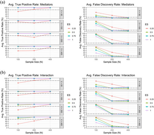
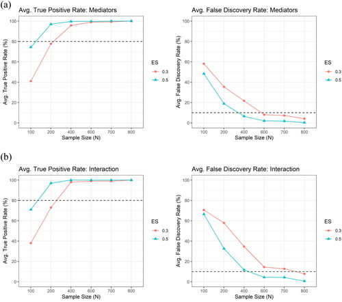
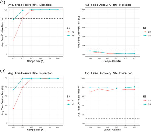
Figure 3 shows the average TPR and the average FDR across the 100 simulation runs by the sample size and the effect size, for (a) the mediator and for (b) the interaction, respectively, under the setting of correlated mediators with correlation structure obtained from Alzheimer’s Disease Neuroimaging Initiative (ADNI) data, using XMInt. By the design of our algorithm, the hierarchical structure between interactions and mediators is preserved (the percentage of interaction without hierarchy were all zeros). When the sample size was large ($N$ at least 600), regardless of the effect size, our algorithm can almost 100% of the time identify all of the three true mediators and the true interaction term (TPR approximately 100%) and it is not likely to falsely select the non-truth (FDRs well controlled under approximately 5% for mediators and 10% for interactions, on average).

Figure 3. The average true positive rate (TPR) and the average false discovery rate (FDR) across the 100 simulation runs by the sample size ($N$) and the effect size ($\mathit{\text{ES}}$), for (a) the mediator (upper panel) and for (b) the interaction (lower panel), respectively, under the setting of correlated mediators with correlation structure obtained from the ADNI data, using XMInt. The number of potential mediators ($V$) is 89, which is the same as in the ADNI data.

By comparison, the hierarchical structure cannot be preserved if we use merely LASSO without adaptive penalties for both settings of mediators—the percentages of selected interaction without hierarchy were high, as shown in Figure 4. Furthermore, as shown in Figures 5 and 6, the FDRs for the interactions were high across all simulation scenarios under both settings of mediators, which indicates that it is likely to falsely select many non-truth interactions using LASSO only.

Figure 4. The average percentage of selected interaction without hierarchical structure across the 100 simulation runs by the sample size ($N$), the number of potential mediators ($V$) and the effect size ($\mathit{\text{ES}}$), under the setting of independent mediators (left) and the setting of correlated mediators with correlation structure obtained from the ADNI data (right), using LASSO only.

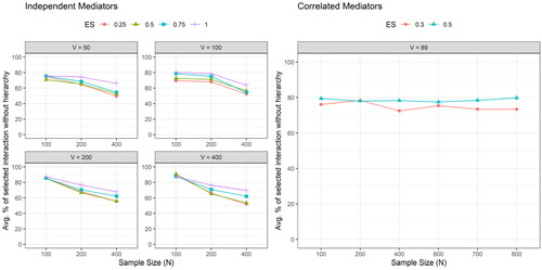
Figure 5. The average true positive rate (TPR) and the average false discovery rate (FDR) across the 100 simulation runs by the sample size ($N$), the number of potential mediators ($V$) and the effect size ($\mathit{\text{ES}}$), for (a) the mediator (upper panel) and for (b) the interaction (lower panel), respectively, under the setting of independent mediators, using LASSO only.

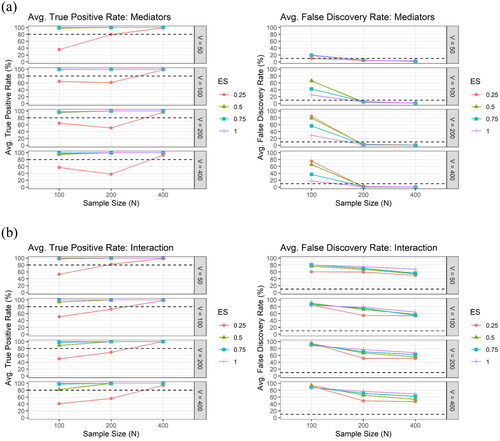
Figure 6. The average true positive rate (TPR) and the average false discovery rate (FDR) across the 100 simulation runs by the sample size ($N$) and the effect size ($\mathit{\text{ES}}$), for (a) the mediator (upper panel) and for (b) the interaction (lower panel), respectively, under the setting of correlated mediators with correlation structure obtained from the ADNI data, using LASSO only. The number of potential mediators ($V$) is 89, which is the same as in the ADNI data.

4. Data Application

We applied our algorithm to the human brain imaging data from the ADNI, a longitudinal multicenter study designed for the early detection and tracking of Alzheimer’s disease. Specifically, we assessed the role of cortical thickness and subcortical volumes on the relationship between amyloid beta accumulation and cognitive abilities at baseline. We used the baseline data from the participants without dementia—diagnosed as mild cognitive impairment (MCI; $N=458$) or cognitively normal (CN; $N=276$). Participants’ characteristics are displayed in Table 2.

Table 2. Participants’ characteristics at baseline (ADNI dataset).

Characteristic	Overall, $N$ = 734^a	CN, $N$ = 276^a	MCI, $N$ = 458^a
Abeta accumulation (pg/mL)	1088.5 (447.3)	1229.3 (440.6)	1003.6 (430.1)
Memory composite scores	0.6 (0.7)	1.1 (0.6)	0.3 (0.7)
Age (years)	71.9 (7.0)	72.8 (5.9)	71.4 (7.6)
Sex
Male	381 (51.9%)	121 (43.8%)	260 (56.8%)
Female	353 (48.1%)	155 (56.2%)	198 (43.2%)
Education (years)	16.3 (2.6)	16.5 (2.5)	16.2 (2.7)
Ethnicity
Hispanic	24 (3.3%)	11 (4.0%)	13 (2.8%)
Not Hispanic	706 (96.2%)	262 (94.9%)	444 (96.9%)
Unknown	4 (0.5%)	3 (1.1%)	1 (0.2%)
Race
White	681 (92.8%)	252 (91.3%)	429 (93.7%)
Non-White	51 (6.9%)	24 (8.7%)	27 (5.9%)
Unknown	2 (0.3%)	0 (0.0%)	2 (0.4%)

Note: CN: cognitively normal; MCI: mild cognitive impairment.

^a n (%); mean (standard deviation).

The data were downloaded from the ADNI database (http://adni.loni.usc.edu). The initial phase (ADNI-1) recruited 800 participants, including approximately 200 healthy controls, 400 patients with late MCI, and 200 patients clinically diagnosed with AD over 50 sites across the United States and Canada and followed up at 6- to 12-month intervals for two to three years. ADNI has been followed by ADNI-GO and ADNI-2 for existing participants and enrolled additional individuals, including early MCI. To be classified as MCI in ADNI, a subject needed an inclusive Mini-Mental State Examination score of between 24 and 30, subjective memory complaint, objective evidence of impaired memory calculated by scores of the Wechsler Memory Scale Logical Memory II adjusted for education, a score of 0.5 on the Global Clinical Dementia Rating, absence of significant confounding conditions such as current major depression, normal or near-normal daily activities, and absence of clinical dementia.

All studies were approved by their respective institutional review boards and all subjects or their surrogates provided informed consent compliant with HIPAA regulations.

The exposure of interest is amyloid beta accumulation, which is a univariate variable. Cerebrospinal fluid (CSF) amyloid beta (A$\beta$-42) concentrations were measured in picograms per milliliter (pg/mL) by ADNI researchers using the highly automated Roche Elecsys immunoassays on the Cobas e601 automated system following extensive validation studies (Bittner et al. 2016; Shaw et al. 2016). The CSF data used in this study were obtained from the ADNI files UPENNBIOMK9_04_19_17.csv. Detailed descriptions of CSF acquisition including lumbar puncture procedures, measurement, and quality control procedures were presented in http://adni.loni.usc.edu/methods/.

The outcome variable of interest is the memory composite score, which is a univariate variable. We used ADNI’s pre-generated cognitive composite scores that were constructed based on bi-factor confirmatory factor analyses models (Crane et al. 2012). Composite memory scores were derived using the Rey Auditory Verbal Learning Test, AD Assessment Schedule-Cognition, Mini-Mental State Examination, and Logical Memory.

MPRAGE T1-weighted MR images were used in this analysis. Cross-sectional image processing was performed using FreeSurfer Version 7.0.1. Region of interest (ROI)-specific cortical thickness and volume measures were extracted from the automated FreeSurfer anatomical parcellation using the Desikan-Killiany Atlas (Desikan et al. 2006) for cortical regions and ASEG (Fischl et al. 2002) for subcortical regions. We considered 89 potential mediators that were derived from 68 cortical thickness measures from both left and right hemispheres, 5 corpus callosum subregion volume measures, and 16 subcortical volume measures from both left and right hemispheres (Thalamus, Caudate, Putamen, Pallidum, Hippocampus, Amygdala, Accumbens, VentralDC). This selection was made because these measures are among the most commonly used measures in AD research. We did not include ventricles and non-brain areas in our analysis as they are surrogate measures of brain atrophy and their volumes do not carry significant biological meaning in this context. While we could use high-resolution measures such as vertex-level cortical thickness measures or voxel-based morphometry (VBM), however, functional data analysis or appropriate dimension reduction is recommended since those measures tend to exhibit much higher correlations. Moreover, it is worth noting that ADNI did administrate other modalities such as DWI, resting fMRI, and ASL, but only to a subset of the participants as per their protocol. Thus, to maintain the largest possible sample size, we decided to use the T1-based measures. Since the volume measures are typically confounded by brain size, we divided them by the estimated total intracranial volume to adjust for the potential confounding effect. Furthermore, as all these 89 measures are often correlated with sex and age, we regressed them on sex and age and used the residuals as our potential mediators.

After the data preparation, data standardization was performed on the exposure, the outcome and the potential mediators such that each of them had a mean of zero and a standard deviation of one, and we used the standardized data in the data analysis. We used the default $K=20$ and $\zeta =0.05$ to generate the $\lambda$ sequence. The regularization parameter for $\mathbf{\Omega }$ estimation ($\gamma$) is fixed at $e^{-1}.$ The final model is given by the $\lambda$ that minimizes HBIC.

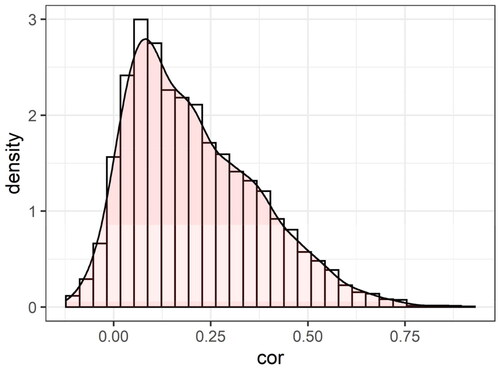
Note that in the simulation of correlated mediators in Section 3, the correlation structure was obtained from the ADNI data. Particularly, the $\mathbf{\Sigma }$ used in the simulation setting of correlated mediators was the correlation matrix of the residuals of the potential mediators after regressing out the effect of the exposure using path-a model, after the data standardization. The average correlation was around 0.2. The distribution of the correlations is also shown in Figure 7.

Figure 7. The distribution of the correlations between the residuals of the 89 potential mediators after regressing out the effect of the exposure using path-a model, after the data standardization, in the ADNI dataset.

Our algorithm identified mediated interaction effects of cortical thickness from two temporal regions: the middle temporal region in the left hemisphere and the superior temporal region in the right hemisphere, as shown in Figure 8. Coefficients are displayed in Table 3 and the HBIC curve is in Figure 9. In other words, the cortical thickness of the two identified regions mediates the relationship between amyloid beta accumulation and cognitive abilities, and further, their effect on cognition is influenced by amyloid beta accumulation. The direction of the interaction can also be explored using the four-way decomposition idea proposed in T. J. VanderWeele (2014), through the regression-based counterfactual approach (Valeri and VanderWeele 2013; VanderWeele T and Vansteelandt 2014) to estimate the joint effect of multiple mediators implemented in CMAverse R package (Shi et al. 2021). Under the counterfactual independence assumptions, it showed that when there is no amyloid beta accumulation, the thinner cortex in the middle temporal region of the left hemisphere and the superior temporal region of the right hemisphere is associated with worse cognitive performance ($\mathrm{\text{PIE}}=0.036,p<.01$); however, when there is more amyloid beta accumulation involved, such mediation effect disappears—the thinner cortex is no longer associated with worse cognition ($\mathrm{\text{TIE}}=0.010,p=.3$). These altogether illustrate the brain compensation mechanism during this process of brain-related changes.

Figure 8. Two cortical thickness measures (one in the middle temporal region in the left hemisphere and the other in the superior temporal region in the right hemisphere) that were identified to have the mediated interaction effects on the relationship between amyloid beta accumulation and memory using XMInt on ADNI dataset.

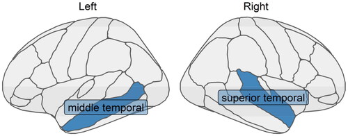
Figure 9. HBIC curve for model selection in ADNI data application for each ${\lambda }_k,k=1,\dots ,20,$ with tuning parameter for $\mathbf{\Omega }\left(\gamma \right)$ fixed at $e^{-1}.$

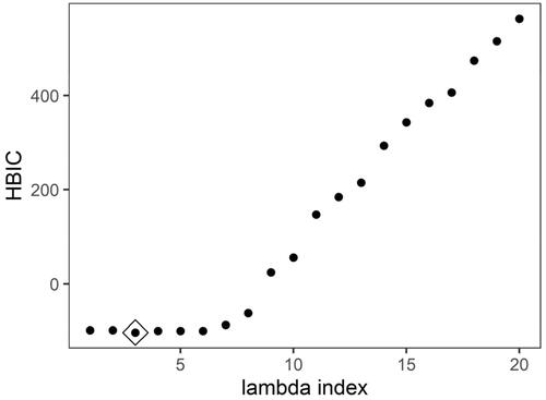
Table 3. Coefficients of selected mediators and exposure-by-mediator interactions in ADNI data application.

	$a$	$b_1$	$b_2$	$c$
Middle temporal thickness (left)	0.0755	0.1100	−0.1278	0.2901
Superior temporal thickness (right)	0.1218	0.0335	−0.1170	0.2901

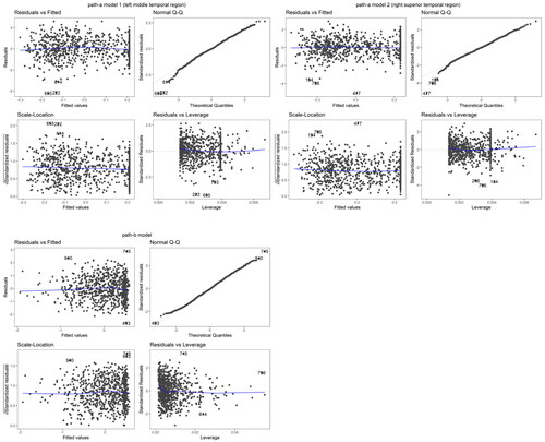
We also performed the model diagnosis to justify the normal assumptions on the model distribution. We fitted the mediation model with the selected two mediators (using the standardized data). As shown in Figure 10, Q-Q plots did not indicate noticeable violation of the normal assumptions on the mediators and the outcome.

Figure 10. The diagnostics plots of the mediation models based on ADNI data analysis results using XMInt.

5. Discussion

In this paper, we proposed the XMInt algorithm to identify the mediators and the exposure-by-mediator interactions in the high-dimensional mediators setting while preserving the underlying hierarchical structure between the main effects and the interaction effects. A key feature of this algorithm is its ability to preserve the hierarchical relationship between the mediators and the exposure-by-mediator interactions. We evaluated the performance of our algorithm under various conditions to investigate when it demonstrates optimal model selection, and two simulation settings of mediators were considered—independent mediators and correlated mediators with correlation structure obtained from the ADNI data—to better mimic real-world situations. Our simulation results revealed that for the independent mediators, when the effect size and the sample size are moderate to large, our algorithm was able to correctly identify the true mediators and interaction almost all the time, without falsely selecting many non-truth variables; a similar conclusion holds for the correlated mediators when the sample size is large, regardless of the effect size. To illustrate our algorithm, we also applied our method to real-world human brain imaging data. Two cortical thickness measures, specifically, one in the middle temporal region in the left hemisphere and the other in the superior temporal region in the right hemisphere, were identified to have mediated interaction effects on the relationship between amyloid beta accumulation and memory abilities. This identification of temporal thickness as a mediator is consistent with the existing literature (e.g., Villeneuve et al. 2014). A follow-up four-way effect decomposition (VanderWeele TJ 2014) revealed that in the absence of amyloid beta accumulation, reduced cortical thickness in these two identified regions is associated with worse cognitive performance, but with increased amyloid beta accumulation, the mediation effect in these two regions disappears, which illustrates a potential brain compensation mechanism. One limitation is that when the number of potential mediators or the sample size becomes larger, it may take a longer time to run the algorithm, as the computation involving $\mathbf{U}$ becomes slower. In summary, our algorithm works well and can be used as an effective tool to identify the mediated interaction with preserved hierarchical structure in the mediation analysis.

Software

The XMInt R package is available at https://github.com/ruiyangli1/XMInt.

Disclosure Statement

No potential conflict of interest was reported by the author(s).

Data availability statement

Data used in the preparation of this article were obtained from the Alzheimer’s Disease Neuroimaging Initiative (ADNI) database (adni.loni.usc.edu), under the data use agreement by ADNI. The simulation experiment data example is available at https://github.com/ruiyangli1/XMInt. As such, the investigators within the ADNI contributed to the design and implementation of ADNI and/or provided data but did not participate in the analysis or writing of this report. A complete listing of ADNI investigators can be found at: http://adni.loni.usc.edu/wp-content/ uploads/how_to_apply/ADNI_Acknowledgement_List.pdf.

Additional information

Funding

This work was supported by the NIH under Grant R01AG062578 (PI: Lee). Data collection and sharing for this project was funded by the Alzheimer’s Disease Neuroimaging Initiative (ADNI) (National Institutes of Health Grant U01 AG024904) and DOD ADNI (Department of Defense award number W81XWH-12-2-0012). ADNI is funded by the National Institute on Aging, the National Institute of Biomedical Imaging and Bioengineering, and through generous contributions from the following: AbbVie, Alzheimer’s Association; Alzheimer’s Drug Discovery Foundation; Araclon Biotech; BioClinica, Inc.; Biogen; Bristol-Myers Squibb Company; CereSpir, Inc.; Cogstate; Eisai Inc.; Elan Pharmaceuticals, Inc.; Eli Lilly and Company; EuroImmun; F. Hoffmann-La Roche Ltd and its affiliated company Genentech, Inc.; Fujirebio; GE Healthcare; IXICO Ltd.; Janssen Alzheimer Immunotherapy Research & Development, LLC.; Johnson & Johnson Pharmaceutical Research & Development LLC.; Lumosity; Lundbeck; Merck & Co., Inc.; Meso Scale Diagnostics, LLC.; NeuroRx Research; Neurotrack Technologies; Novartis Pharmaceuticals Corporation; Pfizer Inc.; Piramal Imaging; Servier; Takeda Pharmaceutical Company; and Transition Therapeutics. The Canadian Institutes of Health Research is providing funds to support ADNI clinical sites in Canada. Private sector contributions are facilitated by the Foundation for the National Institutes of Health (www.fnih.org). The grantee organization is the Northern California Institute for Research and Education, and the study is coordinated by the Alzheimer’s Therapeutic Research Institute at the University of Southern California. ADNI data are disseminated by the Laboratory for NeuroImaging at the University of Southern California.

Appendix A

In this section, we aim to illustrate that the choice of tuning parameter of $\mathbf{\Omega }$ ($\gamma$) does not affect the model selection results significantly, while conducting a grid search for both tuning parameters ($\gamma$ and ${\lambda }_k$’s) can substantially increase computing time, and that our choice of $\gamma =e^{-1}$ in the proposed algorithm is reasonable.

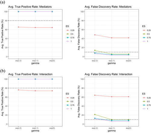
Figure A1 shows the average true positive rate (TPR) and the average false discovery rate (FDR) across the 100 simulation runs, by different values of tuning parameter of $\mathbf{\Omega }$ ($\gamma =e^{-2},e^{-1},e^0$), for (a) the mediator (upper panel) and for (b) the interaction (lower panel), respectively, under the setting of independent mediators with sample size $N=200,$ number of potential mediators $V=200,$ and different effect sizes ($\mathit{\text{ES}}=0.25,0.5,0.75,1$), using XMInt. The results showed that both TPRs and FDRs remained relatively stable across the range of $\gamma$ values. Thus, the value of the regularization parameter for the $\mathbf{\Omega }$ estimation is empirically chosen, following Hsieh et al. (2014), and is fixed at $e^{-1}$ in our simulation study and real-data application.

Figure A1. The average true positive rate (TPR) and the average false discovery rate (FDR) across the 100 simulation runs, by different values of tuning parameter of $\mathbf{\Omega }$ ($\gamma$), for (a) the mediator (upper panel) and for (b) the interaction (lower panel), respectively, under the setting of independent mediators with sample size $N=200,$ number of potential mediators $V=200,$ and different effect sizes ($\mathit{\text{ES}}$), using XMInt.

References

- Baron RM, Kenny DA. 1986. The moderator–mediator variable distinction in social psychological research: conceptual, strategic, and statistical considerations. J Pers Soc Psychol. 51(6):1173–1182.
- Bellavia A, Valeri L. 2018. Decomposition of the total effect in the presence of multiple mediators and interactions. Am J Epidemiol. 187(6):1311–1318.
- Bien J, Taylor J, Tibshirani R. 2013. A lasso for hierarchical interactions. Ann Stat. 41(3):1111–1141.
- Bittner T, Zetterberg H, Teunissen CE, Ostlund RE Jr, Militello M, Andreasson U, Hubeek I, Gibson D, Chu DC, Eichenlaub U, et al. 2016. Technical performance of a novel, fully automated electrochemiluminescence immunoassay for the quantitation of β-amyloid (1–42) in human cerebrospinal fluid. Alzheimers Dement. 12(5):517–526.
- Bollen KA, Harden JJ, Ray S, Zavisca J. 2014. BIC and alternative Bayesian information criteria in the selection of structural equation models. Struct Equ Model. 21(1):1–19.
- Bühlmann P, Van De Geer S. 2011. Statistics for high-dimensional data: methods, theory and applications. Berlin (Germany): Springer.
- Chipman H. 1996. Bayesian variable selection with related predictors. Can J Stat. 24(1):17–36.
- Choi NH, Li W, Zhu J. 2010. Variable selection with the strong heredity constraint and its oracle property. J Am Stat Assoc. 105(489):354–364.
- Crane PK, Carle A, Gibbons LE, Insel P, Mackin RS, Gross A, Jones RN, Mukherjee S, Curtis SM, Harvey D, et al. 2012. Development and assessment of a composite score for memory in the Alzheimer’s disease neuroimaging initiative (ADNI). Brain Imaging Behav. 6(4):502–516.
- Daniel RM, De Stavola BL, Cousens SN, Vansteelandt S. 2015. Causal mediation analysis with multiple mediators. Biometrics. 71(1):1–14.
- Desikan RS, Ségonne F, Fischl B, Quinn BT, Dickerson BC, Blacker D, Buckner RL, Dale AM, Maguire RP, Hyman BT, et al. 2006. An automated labeling system for subdividing the human cerebral cortex on MRI scans into gyral based regions of interest. Neuroimage. 31(3):968–980.
- Fischl B, Salat DH, Busa E, Albert M, Dieterich M, Haselgrove C, Van Der Kouwe A, Killiany R, Kennedy D, Klaveness S, et al. 2002. Whole brain segmentation: automated labeling of neuroanatomical structures in the human brain. Neuron. 33(3):341–355.
- Friedman J, Hastie T, Tibshirani R. 2010. Regularization paths for generalized linear models via coordinate descent. J Stat Soft. 33(1):1–22.
- Gao X, Pu DQ, Wu Y, Xu H. 2012. Tuning parameter selection for penalized likelihood estimation of gaussian graphical model. Stat Sin. 22(3):1123–1146.
- Hamada M, Wu CFJ. 1992. Analysis of designed experiments with complex aliasing. J Qual Technol. 24:3.
- Hao N, Feng Y, Zhang HH. 2018. Model selection for high-dimensional quadratic regression via regularization. J Am Stat Assoc. 113(522):615–625.
- Hao N, Zhang HH. 2017. A note on high-dimensional linear regression with interactions. Am Stat. 71(4):291–297.
- Haughton DM, Oud JH, Jansen RA. 1997. Information and other criteria in structural equation model selection. Commun Stat Simul Comput. 26(4):1477–1516.
- Haughton DMA. 1988. On the choice of a model to fit data from an exponential family. Ann Stat. 16(1):342–355.
- Holland PW. 1988. Causal inference, path analysis, and recursive structural equations models. Sociol Methodol. 18:449–484.
- Hsieh CJ, Sustik M, Dhillon IS, Ravikumar P. 2014. Quic: quadratic approximation for sparse inverse covariance matrix estimation. J Mach Learn Res. 15(1):2911–2947.
- Imai K, Keele L, Yamamoto T. 2010. Identification, inference and sensitivity analysis for causal mediation effects. Stat Sci. 25(1):51–71.
- Imai K, Yamamoto T. 2013. Identification and sensitivity analysis for multiple causal mechanisms: revisiting evidence from framing experiments. Polit Anal. 21(2):141–171.
- Li B, Yu Q, Zhang L, Hsieh M. 2021. Regularized multiple mediation analysis. Stat Interface. 14(4):449–458.
- Lin LC, Huang PH, Weng LJ. 2017. Selecting path models in SEM: a comparison of model selection criteria. Struct Equ Model. 24(6):855–869.
- Luo C, Fa B, Yan Y, Wang Y, Zhou Y, Zhang Y, Yu Z. 2020. High-dimensional mediation analysis in survival models. PLoS Comput Biol. 16(4):e1007768.
- MacKinnon DP. 2008. Introduction to statistical mediation analysis. New York (NY): Routledge.
- Nelder JA. 1977. A reformulation of linear models. J R Stat Soc Ser A. 140(1):48–77.
- Pearl J. 2013. Direct and indirect effects. arXiv:13012300 [cs, stat]. [accessed 2022 Jan 05]. http://arxiv.org/abs/1301.2300.
- Peixoto JL. 1987. Hierarchical variable selection in polynomial regression models. Am Stat. 41(4):311–313.
- Preacher KJ, Hayes AF. 2008. Asymptotic and resampling strategies for assessing and comparing indirect effects in multiple mediator models. Behav Res Methods. 40(3):879–891.
- Robins JM, Greenland S. 1992. Identifiability and exchangeability for direct and indirect effects. Epidemiology. 3(2):143–155.
- Schaid DJ, Sinnwell JP. 2020. Penalized models for analysis of multiple mediators. Genet Epidemiol. 44(5):408–424.
- Serang S, Jacobucci R, Brimhall KC, Grimm KJ. 2017. Exploratory mediation analysis via regularization. Struct Equ Model. 24(5):733–744.
- Shaw LM, Fields L, Korecka M, Waligórska T, Trojanowski JQ, Allegranza D, Bittner T, He Y, Morgan K, Rabe C. 2016. Method comparison of ab (1-42) measured in human cerebrospinal fluid samples by liquid chromatography-tandem mass spectrometry, the inno-bia alzbio3 assay, and the elecsys® b-amyloid (1-42) assay. Alzheimers Dement. 7(12):P668.
- Shi B, Choirat C, Coull BA, VanderWeele TJ, Valeri L. 2021. CMAverse: a suite of functions for reproducible causal mediation analyses. Epidemiology. 32(5):e20–e22.
- Sobel ME. 2008. Identification of causal parameters in randomized studies with mediating variables. J Educ Behav Stat. 33(2):230–251.
- Valeri L, VanderWeele TJ. 2013. Mediation analysis allowing for exposure-mediator interactions and causal interpretation: theoretical assumptions and implementation with SAS and SPSS macros. Psychol Methods. 18(2):137–150.
- VanderWeele T. 2015. Explanation in causal inference: methods for mediation and interaction. Oxford University Press.
- VanderWeele T, Vansteelandt S. 2014. Mediation analysis with multiple mediators. Epidemiol Methods. 2(1):95–115.
- VanderWeele TJ. 2011. Controlled direct and mediated effects: definition, identification and bounds. Scand Stat Theory Appl. 38(3):551–563.
- VanderWeele TJ. 2014. A unification of mediation and interaction: a four-way decomposition. Epidemiology. 25(5):749–761.
- van Kesteren EJ, Oberski DL. 2019. Exploratory mediation analysis with many potential mediators. Struct Equ Model. 26(5):710–723.
- Villeneuve S, Reed BR, Wirth M, Haase CM, Madison CM, Ayakta N, Mack W, Mungas D, Chui HC, DeCarli C, et al. 2014. Cortical thickness mediates the effect of β-amyloid on episodic memory. Neurology. 82(9):761–767.
- Wainwright MJ. 2009. Sharp thresholds for high-dimensional and noisy sparsity recovery using ℓ1 -constrained quadratic programming (lasso). IEEE Trans Inform Theory. 55(5):2183–2202.
- Wang C, Hu J, Blaser MJ, Li H. 2020. Estimating and testing the microbial causal mediation effect with high-dimensional and compositional microbiome data. Bioinformatics. 36(2):347–355.
- Wang Y, Bernanke J, Peterson BS, McGrath P, Stewart J, Chen Y, Lee S, Wall M, Bastidas V, Hong S, et al. 2019. The association between antidepressant treatment and brain connectivity in two double-blind, placebo-controlled clinical trials: a treatment mechanism study. Lancet Psychiatry. 6(8):667–674.
- Yuan M, Joseph VR, Zou H. 2009. Structured variable selection and estimation. Ann Appl Stat. 3(4):1738–1757.
- Zhang H, Zheng Y, Hou L, Zheng C, Liu L. 2021. Mediation analysis for survival data with high-dimensional mediators. Bioinformatics. 37(21):3815–3821.
- Zhang H, Zheng Y, Zhang Z, Gao T, Joyce B, Yoon G, Zhang W, Schwartz J, Just A, Colicino E, et al. 2016. Estimating and testing high-dimensional mediation effects in epigenetic studies. Bioinformatics. 32(20):3150–3154.
- Zhao P, Rocha G, Yu B. 2009. The composite absolute penalties family for grouped and hierarchical variable selection. Ann Stat. 37(6A):3468–3497. http://arxiv.org/abs/0909.0411.
- Zhao Y, Lindquist MA, Caffo BS. 2020. Sparse principal component based high-dimensional mediation analysis. Comput Stat Data Anal. 142:106835.
- Zhao Y, Luo X. 2016. Pathway lasso: estimate and select sparse mediation pathways with high dimensional mediators. arXiv:160307749 [stat]. [accessed 2021 Nov 16]. http://arxiv.org/abs/1603.07749.