Bayesian Systemic Risk Analysis using Latent Space Network Models

Abstract

In financial markets, systemic risk is a type of risk in which the failure of one stock in the market triggers a sequence of failures. Our study proposes a Bayesian decision scheme to dynamically monitor systemic risk under any preferences and restrictions in financial risk management. We begin by capturing the moving correlations of stock returns because such correlations represent the strengths of the relationships among stocks. Then, we construct a dynamic financial network to link the stocks with strong relationships. Using the financial space, which is related to the position of stocks in the network plot, we locate two stocks in the financial space that are a short distance apart, because the relationship between these two stocks is strong. Using the distances between stocks in the financial space, together with the salient preferences and restrictions in financial risk management, we propose a systemic risk score. We then use 20 years of data to demonstrate the effectiveness of our proposed systemic risk score to give an early signal of global financial instabilities.

Keywords:

• Dynamic networks
• latent space model
• Monte Carlo Markov chain
• network connectedness
• risk management
• systemic risk

1. Introduction

Systemic risk describes a chain of failures among institutions or markets that is triggered by contagion from a failure in one of them (Chan et al. 2005). Compared with the failure of an individual institution, we might think it unlikely that many institutions could fail simultaneously. However, institutions can never isolate themselves from external influences (Bhar and Nikolova 2013; Raddant and Kenett 2021), and the relationships among the institutions, as one source of systemic risk, can transfer a failure from one to another. Even if the initial shock is created by the failure of one institution, it can create a chain of breakdowns when the relationships among institutions are strong (Contreras et al. 2022). The subprime mortgage crisis in 2008 (Dwyer and Tkac 2009; Tomczak 2023) is a well-known global incident demonstrating the importance of studying systemic risk in the markets. A market crash will also induce a high level of systemic risk—such as the crash of 2020, which was brought about by the COVID-19 pandemic (So et al. 2021b). Regional incidents, too, including the European sovereign debt crisis (Ureche-Rangau and Burietz 2013) and the war in Ukraine (Lockett 2022), affect not only the local markets but also the global market, and research on the immediate impact and aftershocks of these crises is still ongoing. In this paper, we develop a new approach for measuring systemic risk over time that incorporates a variety of financial risk-management scenarios.

Extensive research has suggested several possible directions (De Bandt and Hartmann 2000; Benoit et al. 2017) for the study of systemic risk. One direction focuses on balance sheets and macroeconomic data (Jackson and Pernoud 2021), with the balance sheet approach reflecting major businesses’ relationships with other institutions (Hanson et al. 2011; Haldane and May 2011; Cai et al. 2018), while the macroeconomic data approach reflects the market situation (Brunnermeier 2009; Rodríguez-Moreno and Peña 2013; He and Krishnamurthy 2019). Another direction focuses on textual information (Maiya and Rolfe 2014; Kawata and Fujiwara 2016; So et al. 2022), extracting real-time financial news and building a network based on keywords to track the market situation.

Our proposal for the study of systemic risk focuses on the relationships revealed by daily stock returns. We assume that, if a business relationship exists between two institutions, any news concerning one of them will affect the stock returns of both. Therefore, by capturing the correlations of stock returns (De Nicolo and Kwast 2002; Blei and Ergashev 2014), we can measure the strength of the business relationship between those two institutions. When the relationships among institutions in the market are strong, any bad news about one member of the market can trigger a chain reaction of failures (Mantegna and Stanley 1999). Therefore, it is important to detect the pairs of institutions that possess a strong relationship (Battiston et al. 2012; Thurner and Poledna 2013; Huang et al. 2013; So et al. 2021a).

In the literature, several useful statistics are aimed at using stock returns to detect the relationships between institutions and market crashes, including but not limited to systemic expected shortfalls (SES) (Acharya et al. 2017), SRISK (the expected capital shortfall of a financial entity, conditional on a prolonged market decline) (Brownlees and Engle 2017), $\Delta$ CoVaR (the value at risk (VaR) of the financial system, conditional on institutions being under distress) (Adrian and Brunnermeier 2016), and Absorption Ratio (AR), which measures supply and demand (Kritzman et al. 2011). Using statistical models to capture the instability contributed by the relationships among institutions is also possible (Girardi and Ergün 2013; So et al. 2020a, 2021c). Some studies have analyzed the market situation by using network statistics (Tabak et al. 2014; Wang et al. 2017; Neveu 2018; So et al. 2021a; Lai and Hu 2021; So et al. 2021b). As a further development on these approaches, Billio et al. (2012) constructed a systemic risk measure using principal component analysis and a network of Granger-causality. Hautsch et al. (2015) studied the realized systemic risk (volatility) beta value, using the significant relationship in the tail event, along with information from the market and balance sheets. Diebold and Yılmaz (2014) considered the variance decomposition technique to construct a network to measure systemic risk. Wang et al. (2021) considered a multilayered network to handle various types of stock information in detecting systemic risk. Härdle et al. (2016) considered the network-analysis-based tail event on stock returns.

As with the work of some others, our proposal involves Bayesian methods in the computation of systemic risk—such use is not new. Gandy and Veraart (2017) considered a weighted directed network that measured individual liabilities among institutions. Ballester et al. (2023) studied the transmission of systemic credit risk by using a Bayesian network. Lupu et al. (2020) estimated some common systemic risk measures with a Bayesian entropy estimation method. Deng and Matteson (2022) proposed the Bayesian Spillover Graphs to study the dynamic network and identify some special features of the network.

Specifically, the proposed systemic risk measurement is based on the work of Das (2016), and two components constitute our score. First, we assign a weight to each institution with the Bayesian framework. In application, investors may for example have a greater concern about systemic risk among the institutions that belong to a particular industry, and the relationships among institutions in that industry should be the focus, even though the business relationships of others also deserve attention. Another example would be an investor who faces restrictions on investments or has preferences for systemic risk management; the proposed systemic risk score has set up a weight with the Bayesian framework to adjust to those restrictions and preferences.

In addition to the weight assigned to each stock, we aggregate information from the pairwise relationships of institutions, to measure their contribution to systemic risk. We consider a network model that represents the institutions as nodes and the significance of business relationships by edges. When an institution fails, the impact first transfers to those who have a business relationship with the failed institution. Depending on the strength of their relationship to the failed institution and the loss in that impact, other institutions might then generate the next impact and transfer it to a further institution, which may not be directly linked to the source of the first impact (Martínez-Jaramillo et al. 2010; Aiyar 2012; Acemoglu et al. 2015). Therefore, a network model that highlights those strongly related institutions accounts for the contagion of failure resulting from connectedness in the market (Chen et al. 2020).

Although a network model explores and visualizes significant business relationships, our study builds further upon the financial network with a latent space, extending the concept of the latent space from Chu et al. (2021). The latent space converts the binary indicator in the network—whether or not a pair of institutions is significantly related—to a continuous measure of the likelihood that a pair of institutions is related. The latent space includes all of the institutions as points and assigns each one’s position such that the distance between two points reflects the significance of their relationship to all other institutions in the latent space. An advantage of using the latent space model over simply a network model is that the distances in latent space can provide hints that indicate the indirect relationships between two institutions, formed by a chain of institutions, by assigning a short distance between the institutions, while the distance in a network—that is, the length of the shortest path between institutions—may miss it. Some studies visualize the network and make use of the arrangement of positions in the visualization to measure systemic risk (Heimo et al. 2007; Linardi et al. 2020). We have chosen a Bayesian approach to look for the best position in the latent space. Combining these two components, then, we take the weights of each institution and the network with an embedded latent space, or what we call the financial space, since the space is related to financial information, as input into the systemic risk score.

To the best of our knowledge, we are the first to combine a Bayesian framework for weight assignments and the concept of a financial network with an embedded latent space. As an application of the systemic risk score, we attempt to construct an early signal that warns of impending market crashes. We consider the stock return data in the Hong Kong market for the past 20 years and use the systemic risk score to detect any prior signal of the financial turnulence during that period. We also compare the model’s performance in raising an early signal with that of other well-known systemic risk measures. In the literature, Billio et al. (2016) proposed an early signal based on entropy measures with the financial market in Europe. Allaj and Sanfelici (2022) used realized variance and the feedback rate of price volatility to construct an early signal. We examine our proposed model by considering dynamic time wrapping, which matches the pattern of two time series, to determine the lead and lag relationships. When the systemic risk score leads the market returns before and during the crashes at a reasonable distance, we say that the systemic risk score has raised an early signal predicting the market crashes. We also use the systemic risk score to demonstrate various applications for establishing the weight of each institution in the Bayesian framework. We demonstrate that our approach overcomes the difficulties in determining a representative weight under complex risk-management restrictions and preferences.

In the remainder of this paper, Section 2 describes the study’s methods and materials and the details and setup of the two components of the proposed systemic risk score, and lists other systemic risk measures for comparison. Section 3 describes the approach to estimate the model parameters and the relevant settings. Section 4 describes the experimental approach, the results of the comparison, and some properties of the systemic risk score. Section 5 discusses the results, summarizes the limitations of our model, and proposes possible directions for future research.

2. Materials and Methods

2.1. Systemic Risk Score

Suppose there are n stocks in the financial market of interest. Our proposed systemic risk score takes two inputs, the first of which is the weight ${\omega }_i$ of stock i in measuring the systemic risk, for $i=1,\dots ,n.$ Because the weights determine the amount of attention we pay to each stock, the purpose of calculating systemic risk determines how we should assign the weights. Let $\omega =({\omega }_1\dots {\omega }_n)$ be the vector of weight. In our study, we made two assumptions on the weights:

1. All entries in $\omega$ are non-negative, and

2. The sum of all entries of $\omega$ equals 1.

The first assumption is required to ensure that the systemic risk score is well-defined. Following this assumption, a zero weight for stock i means that the stock i receives minimum attention or is not being considered when measuring systemic risk. The second assumption is not compulsory. This assumption says that we measure the attention to each stock in a relative sense, instead of in an absolute sense. This is also helpful when we compare the systemic risk score across scenarios. For example, suppose that we treat the weights as the amount of assets allocated to each stock. The systemic risk score will be proportional to the total capital, even if the proportion of assets allocated to each stock is identical. Only when we put the weights on the same scale will the comparison across portfolios become meaningful.

The next input to the proposed systemic risk is the contribution of systemic risk $c_{i,j}$ given by the relationship between stock i and j. As explained in the Introduction, strong relationships between stocks build the path toward a failure contagion. We assign the value of $c_{i,j}$ according to the strength of the relationship, accounting not only for the direct connection but also for the indirect connection, which is linked through a chain of intermediates.

We make use of the significance of the business relationships between stocks, together with the importance of the stocks, to construct the systemic risk scores. Let $C=(c_{i,j})$ is a matrix of systemic risk contributions given by the pairwise relationships of stocks. Our systemic risk score is defined by $S(\omega ,C),$ a function of both the weights and the systemic risk contributions. There are many possible formulations for systemic risk, but motivated by Das (2016), we select those with the following properties:

1. S has to be non-negative. In particular, when $\omega =0,$ the systemic risk score $S(\omega ,C)=0.$

2. When $c_{i,j}$ increases, S increases.

3. S is continuously differentiable on the weight $\omega$ and is also linearly homogeneous of order 1.

The first property ensures a natural representation of risk: If we do not put weight on any asset, the systemic risk in our consideration must be 0. The second property follows directly from the meaning of the matrix C: The higher the contribution given by the relationship of a pair of stocks, the higher the systemic risk. The third property is helpful for understanding the proposed systemic risk score. This property ensures that scaling all of the weights by a positive factor will scale the $S(\omega ,C)$ by the same factor.

Hence, according to Euler’s homogeneous function theorem, we decompose the systemic risk into the sum product of the partial derivatives and the weights. (1) $$S(\omega ,C)=\sum _{i=1}^n\frac{\partial S}{\partial {\omega }_i}{\omega }_i.$$(1)

Based on Equation (1)(1) $$S(\omega ,C)=\sum _{i=1}^n\frac{\partial S}{\partial {\omega }_i}{\omega }_i.$$(1) , the partial derivative with respect to ${\omega }_i$ represents the change in systemic risk per unit weight contributed by a small change in weight. If the partial derivative is large, stock i will have a large influence on the systemic risk. This happens when the relationships between stock i and some other stocks contribute significantly to the systemic risk, and consequently, those stocks should be the focus of our attention. Therefore, we adopt the systemic risk score S in this study, so that (2) $$\frac{\partial S}{\partial {\omega }_i}=\frac{1}{S}\sum _{j=1}^n{c}_{i,j}{\omega }_j.$$(2)

The fraction $1/S$ in Equation (2)(2) $$\frac{\partial S}{\partial {\omega }_i}=\frac{1}{S}\sum _{j=1}^n{c}_{i,j}{\omega }_j.$$(2) is necessary for the third property. Putting the partial derivatives and the weights together, we have (3) $$S(\omega ,C)=\sqrt{{\omega }^{\top }C\omega }$$(3) $$\begin{array}{cc}=\hfill & \sqrt{\sum _{i=1}^n\sum _{j=1}^n{c}_{i,j}{\omega }_i{\omega }_j}.\hfill \end{array}$$

Because there is a square root outside the quadratic form ${\omega }^{\top }C\omega ,$ we need to guarantee that the sum inside the square root of Equation (3)(3) $$S(\omega ,C)=\sqrt{{\omega }^{\top }C\omega }$$(3) is positive. A sufficient condition is to require C to be positive semi-definite. In our case, because the weights are non-negative, we only require all entries of C to be non-negative.

2.2. Bayesian Decision Theory Applied to Various Financial Scenarios

The assignment of weights $\omega$ – that is, of the attention we pay to each stock—depends on the situation. For example, if we care about the systemic risk encountered in a particular portfolio, we can set the weights as the proportion of assets allocated to each stock. We can always find the optimal allocation by minimizing the systemic risk score. However, in a case in which there are some restrictions or limitations on the weight selection, instead of looking for an optimal allocation, we are interested in studying how these restrictions affect the systemic risk.

Therefore, instead of looking for a single weight to represent the financial scenario, we produce multiple values for systemic risk, one on each possible combination of weights. This approach coincides with the framework of Bayesian decision theory (Rachev et al. 2008; Ando 2009). We assign a distribution to the weights $\omega$ and then study the distribution of systemic risk score defined in Equation (3)(3) $$S(\omega ,C)=\sqrt{{\omega }^{\top }C\omega }$$(3) . This approach bypasses the difficulties of looking for a weight that represents the scenario. Adopting the Bayesian decision process also gives us flexibility in setting the level of importance of each of the possible weights. Although multiple weights are available under the constraints, some of them are in favor of the market participants. The level of importance distinguishes the amount of emphasis put upon each of the weights, which in the framework of Bayesian decision theory is equivalent to setting an informative prior for the weights. Correspondingly, the prior density takes on the role of the level of importance.

Throughout our paper, we assign two kinds of distribution to the prior for the weights. We emphasize that other distributions are also possible, as long as they fit the financial scenario and the preference toward each combination of weights. The level of importance, or equivalently the prior density, assigned to each combination of weights, is determined by the hyperparameter, regardless of the choice of distribution. Therefore, the specification of hyperparameters is also important in setting up the financial scenario of interest.

The first distribution is the Dirichlet distribution. This distribution matches the two assumptions on the weights in Section 2.1 when there is no further restriction on the collection of possible combinations of weights. The hyperparameter of the Dirichlet distribution $\alpha =({\alpha }_1\dots {\alpha }_n)$ is a vector of length n, is positive in all entries, and determines the mean and variance of the weights $\omega .$ We have three specifications of hyperparameters to be considered in our study.

1. Random Allocation.

   In a random allocation, every possible combination of weights has the same level of importance—such as taking every entry of $\alpha$ as 1. This is the baseline specification for most financial scenarios in our study because this specification is equivalent to no preference for any particular combination of weights.

2. Allocation proportional to market capitalization.

   In an allocation that is proportional to market capitalization, the mean of weights $\omega$ is proportional to the market capitalization shared by each stock. Market capitalization is the total dollar value of a stock. When a company with a large weight fails, it impacts the market severely and leads to a series of failures. This is achieved in the model by setting the proportion of ${\alpha }_i$ shared by the sum of all entries in $\alpha$ to be proportional to the market capitalization shared by stock i. Therefore, we have to set the sum of $\alpha$ to complete the specification. Notice that when ${\alpha }_i$ is smaller than 1, those combinations of weights that have ${\omega }_i$ deviating from the prior mean receive a higher level of importance. To avoid this counter-intuitive case, we assign the sum of $\alpha$ so that the smallest ${\alpha }_i$ is 1. We compare this specification with the random allocation as one financial scenario in our study.

3. Allocation including a risk-free asset.

   In an allocation that includes a risk-free asset, one extra stock, representing the risk-free asset, is inserted into the consideration. Therefore, now we have $n+1$ entries for the weight $\omega =({\omega }_1\dots {\omega }_{n+1}),$ and so for the hyperparameter of the Dirichlet distribution, $\alpha =({\alpha }_1\dots {\alpha }_{n+1}).$ The contribution of systemic risk toward the risk-free asset and any other asset is set to be 0. While holding all other entries of $\alpha$ constant, increasing the value of ${\alpha }_{n+1}$ decreases the weights that are assigned to risky assets and hence reduces the systemic risk score. At one extreme, when the weight of the risk-free asset ${\omega }_{n+1}$ is 1, the systemic risk score achieves 0, which is the minimum value of the score. At the other extreme, when ${\omega }_{n+1}$ is 0, the systemic risk score is equivalent to ignoring the risk-free asset. As one financial scenario in our study, we compare this specification with the random allocation to study the effect that a decreasing systemic risk score has on increasing ${\alpha }_{n+1}.$

   The second distribution to the prior for the weights is a joint of multiple independent scaled Dirichlet distributions. This is the distribution of weights when each stock is pre-assigned into exactly one of the G groups, and the sum of the weights of stocks in each group is predetermined. We let ${\omega }_{(g)}$ be the vector of the weight of stocks that belong to group g, and ${\omega }_{(g)}^{+}$ is the sum of the weight of stocks in group g. Hence, we have ${\omega }_{(g)}/{\omega }_{(g)}^{+}$ as the proportion of the predetermined sum of weights of stocks in group g being assigned to each stock in group g. Therefore, by setting each ${\omega }_{(g)}/{\omega }_{(g)}^{+}$ to be Dirichlet distributed with hyperparameter ${\alpha }_{(g)},$ we have the weight $\omega$ following a joint of multiple independently scaled Dirichlet distributions. We have three specifications of the hyperparameter to consider in our study.

4. Allocation with an equally shared industry sum of weights.

   In an allocation with an equally shared industry sum of weights, we first classify the stocks according to their industry. Within each group, we use a random allocation—that is, we take every entry of ${\alpha }_{(g)}$ as 1, to specify that there is no preference within the group. We equally share the sum of weights with each group, so that the sum of weights in each group is $1/G.$ This specification is the baseline for the allocation with weights competition within groups.

5. Allocation with the industry of focus.

   In the allocation with an equally shared industry sum of weights, we have set the sum of weights in each group to be $1/G.$ To indicate a focus on an industry-specific crisis, we set a sum of weights for the industry of concern to be 0.5 and each of the remaining industries shares the remaining sum of weights equally, at $0.5/(G-1).$ We compare the systemic risk score of a focus on the industry-specific crisis with the random allocation.

6. Allocation with a weights competition within groups.

   In the allocation with an equally shared industry sum of weights, we make use of the random allocation and state no preference for any combination of weights within each group. In this specification of an allocation with a weights competition within groups, stocks compete for weights within their group. We achieve this by taking every entry of ${\alpha }_{(g)}$ as 0.1. Because all entries of ${\alpha }_{(g)}$ are less than 1, those combinations where the weights deviate from the prior mean receive a higher level of importance. Under the constraint that the sum of all entries of ${\omega }_{(g)}$ is 1, the combination of weights in which one of the stocks takes the majority of weights while the remaining stocks share the remaining proportion receives a higher level of importance than does the combination of weights in which each stock equally shares the weights. Therefore, the stocks in each group prefer to compete instead of share the weights. We compare the systemic risk score under this specification with the allocation with an equally shared industry sum of weights.

2.3. Setting up the Contribution of Systemic Risk with a Latent Space Model

The next input to the systemic risk score is the contribution of systemic risk given by the business relationship between two institutions. Information on the relationships between institutions is often inaccessible however, and even if we can gain access to the data, it is still not easy to determine the contribution to systemic risk given specifically by the two institutions’ relationship. Therefore, we need a proxy for the relationship between the two institutions. In our study, we choose the correlation of stock returns as our proxy. We believe that if two institutions have a significant relationship, whenever one of them suffers and its stock returns fall, the other one will also be impacted. We therefore first use the stock returns to construct a network of significant business relationships. Then, we embed a financial space into the network to further study the indirect business relationships, which are relationships created through a sequence of intermediate institutions (Ng et al. 2021).

2.3.1. Network Setup

We study the strength of the relationships by considering the correlations between the stock returns (Chen et al. 2020; Patro et al. 2013). Suppose our dataset of stock contains information of T trading days in total. Let $p_{i,t}$ is the closing price of stock $i=1,\dots ,n$ on day t. The log return (4) $$r_{i,t}=\hspace{0.17em}\mathrm{\text{log}}\hspace{0.17em}(p_{i,t})-\hspace{0.17em}\mathrm{\text{log}}\hspace{0.17em}(p_{i,t-1})$$(4) is the difference in the log price on two consecutive trading days. Let ${\overline{r}}_{i,t}$ be the 21-days historical average log return of stock i on day t – that is, (5) $${\overline{r}}_{i,t}=\frac{1}{21}\sum _{h=0}^{20}{r}_{i,t-h}.$$(5)

If the sample correlation of the 21-day historical log return between two distinct stocks i and j on day t (6) $${\mathit{\text{Corr}}}_t(i,j)=\frac{\sum _{h=0}^{20}(r_{i,t-h}-{\overline{r}}_{i,t})(r_{j,t}-{\overline{r}}_{j,t-h})}{\sqrt{\sum _{h=0}^{20}{(r_{i,t-h}-{\overline{r}}_{i,t})}^2}\sqrt{\sum _{h=0}^{20}{(r_{j,t}-{\overline{r}}_{j,t-h})}^2}}$$(6) exceeds a threshold, we say the relationship between stocks i and j on trading day t is strong and we assign $y_{i,j,t}=1;$ otherwise, we set $y_{i,j,t}=0.$ Correlations of the 21-day historical average log return are significantly positive at $10\%,$ $5\%,$ and $1\%$ when ${\mathit{\text{Corr}}}_t(i,j)$ is at least 0.2914, 0.3687, 0.5034, respectively. We consider these three critical values as the thresholds in our study.

For each trading day t, we gather all $y_{i,j,t}$ over i and j to form an adjacency matrix $y_t$ so that we put an edge between the nodes representing stocks i and j in the network of the day t if $y_{i,j,t}=1.$ Because the correlation is symmetric—that is, ${\mathit{\text{Corr}}}_t(i,j)={\mathit{\text{Corr}}}_t(j,i)$—the dynamic network is a sequence of undirected networks. Also, we do not assign any value to $y_{i,i,t},$ as we do not include the self-loop in the analysis.

2.3.2. Financial Space

The financial network assigns edges to indicate significant business relationships between institutions. To quantify the contribution of systemic risk, we introduce the concept of financial space, which is latent, unobserved, and D-dimensional. We first let $z_{i,t}={(z_{i,t,1}\dots z_{i,t,D})}^{\top }$ be the coordinates of stock i in the financial space on trading day t. The financial space is a low-dimensional representation of the relationship among those stocks. In particular, the distance between two institutions in the financial space serves as a measurement of the strength of the relationship. Moreover, to have a better understanding of the distance between nodes, we follow a typical choice of $D=2,$ i.e. restricting our attention to a two-dimensional financial space, in the sequel (Sewell and Chen 2015). As a remark, in literature, some studies pick other choices of D when they are considering a more complex network (Zhang et al. 2022).

To give meaning to the distances, we consider a typical network plot that assigns the node positions to give a uniform length of edges and distribution of nodes, to avoid any crossing or blending of edges (Battista et al. 1994). This is often achieved by adopting a network configuration that assigns a shorter distance between those nodes that are more strongly related, and vice versa. To assess the systemic risk on each trading day t, we borrow the concept of “the shorter the distance, the stronger the relationship,” to give meaning to the distance between nodes i and j on the plot of the network corresponding to trading day t.

The financial space is a latent space, meaning that we measure the distance between institutions by considering their relative positions. By embedding the financial space into the network, we assign the nodes in the plot that match their position in the financial space. Therefore, instead of assigning the distances from observed information, we first locate each node in the financial space and then measure the distance between the two nodes. Unlike the nodes and edges in the networks, the financial space is latent and we do not observe the positions directly from the correlations or the network; therefore, we apply the technique of latent space modeling (Hoff et al. 2002; Sewell and Chen 2015; Chu et al. 2021) to find the positions that best represent the systemic risk in the market. The latent space modeling technique for a network aims to use a metric space, usually a two-dimensional Euclidean space, to explain the existence of edges between nodes in a network, and hence to explore the relationships between nodes.

Previous studies have used the nodes-distance measure to calculate connectedness among banks (Cai et al. 2018; Abbassi et al. 2017). By employing the distance measure, we can account for the relationship between nodes. Therefore, from the perspective of an individual stock, the closer it is to other nodes, the higher its chance of suffering contagion from the failure of those neighboring nodes. From the perspective of the market, the shorter the distance between stocks, the easier it is for financial incidents to initiate a contagion of failure, thereby triggering a systemic breakdown.

We then measure the distance between stocks i and j on day t by (7) $$d_{i,j,t}=\left|\left|z_{i,t}-z_{j,t}\right|\right|,$$(7) where $\left|\right|·\left|\right|$ is the Euclidean norm. Recall that the financial space is latent and unobserved. We need some rules to guide ourselves when looking for a position for each stock.

First, for each trading day, we aim to maintain an identical spread of positions. In other words, before considering any data, the positions of stocks on any trading day should have an identical distribution.

After the first day, we determine the positions for trading day t based on the positions from the previous trading day. To maintain an identical spread, we assume that stocks move from their previous positions with a suitable shrinkage towards the center. The center represents the average position that a stock holds throughout the entire study period. Additionally, we introduce the persistence parameter matrix $\Gamma$ to quantify the extent to which information from trading day $t-1$ influences the positions on the current day. A larger value of the persistence parameter indicates a stronger influence of the positions from the last trading day on the current positions.

Let diagmat be a function that creates a diagonal matrix with its diagonal entries arranged in the same sequence as the input, ${\mu }_i={({\mu }_{i,1},\dots ,{\mu }_{i,D})}^{\top }$ represents the average position of stock i throughout the entire study period, ${\tau }_i=\mathit{\text{diagmat}}({\tau }_{i,1},\dots ,{\tau }_{i,D})$ is a diagonal matrix that measures the transition sizes of the positions of stock i in the financial space between consecutive trading days, and ${\Gamma }_i=\mathit{\text{diagmat}}({\rho }_{i,1},\dots ,{\rho }_{i,D})$ is also a diagonal matrix that measures the persistence of stock i. On day $t=1,$ we assume that the position for stock i follows a D-variate normal distribution: (8) $$z_{i,1}\sim N({\mu }_i,{(I-{\Gamma }_i^2)}^{-1}{\tau }_i^2),$$(8) where I is the identity matrix. After the first day, the position of stock i on trading day t is determined as follows: (9) $$z_{i,t}|z_{i,t-1}\sim N({\mu }_i+{\Gamma }_i(z_{i,t-1}-{\mu }_i),{\tau }_i^2).$$(9)

For each stock i and dimension d, we consider the sequence $\{z_{i,1,d},\dots ,z_{i,T,d}\}$ as a univariate autoregressive time series of order 1. To ensure an identical variance over all the marginal distribution of the position in all t, we set the initial spread as ${(I-{\Gamma }_i^2)}^{-1}{\tau }_i^2,$ as shown in Equation (8)(8) $$z_{i,1}\sim N({\mu }_i,{(I-{\Gamma }_i^2)}^{-1}{\tau }_i^2),$$(8) , and restrict ${\rho }_{i,d}\in [0,1)$ for all i and d.

The setup in Equations (8)(8) $$z_{i,1}\sim N({\mu }_i,{(I-{\Gamma }_i^2)}^{-1}{\tau }_i^2),$$(8) and (9)(9) $$z_{i,t}|z_{i,t-1}\sim N({\mu }_i+{\Gamma }_i(z_{i,t-1}-{\mu }_i),{\tau }_i^2).$$(9) indicates that the position of stocks across dimension are independent. Therefore, equivalent to Equations (8)(8) $$z_{i,1}\sim N({\mu }_i,{(I-{\Gamma }_i^2)}^{-1}{\tau }_i^2),$$(8) and (9)(9) $$z_{i,t}|z_{i,t-1}\sim N({\mu }_i+{\Gamma }_i(z_{i,t-1}-{\mu }_i),{\tau }_i^2).$$(9) , the position of stock i on dimension d on day 1 is (10) $$z_{i,1,d}\sim N\left({\mu }_{i,d},{\left(1-{\rho }_{i,d}^2\right)}^{-1}{\tau }_{i,d}^2\right),$$(10) and the position of stock i on dimension d on day $t>1$ is (11) $$z_{i,t,d}|z_{i,t-1,d}\sim N\left({\mu }_{i,d}+{\rho }_{i,d}(z_{i,t-1,d}-{\mu }_{i,d}),{\tau }_{i,d}^2\right).$$(11)

2.3.3. Potential factors for Strong Relationships between Stocks

Multiple potential factors affect the chance for two stocks to be strongly related. In our study, we classify the stocks into $M=4$ groups by industry: Finance $(m=1),$ Utilities $(m=2),$ Properties $(m=3),$ and Commerce & Industry $(m=4).$

Stocks from the same industry share some common characteristics, thus inflating the correlations of their returns. However, any common characteristic is only limited to those within the same industry, so the inflation applies only to those pairs of stocks belonging to the same industry. The extra risk due to the common characteristic results in different probabilities when comparing a pair of stocks coming from the same industry to another pair coming from two different industries. In other words, if both stocks i and j come from industry m on trading day t, we assign $X_{i,j,t,m}=1.$ Otherwise, if stocks i and j come from two different industries, we set $X_{i,j,t,m}=0.$

2.3.4. Forming a Network of Significant Business Relationships

We use the financial space and other potential factors to explain the significance of the relationship between two stocks. In our study, the significance of a business relationship depends on whether the correlation of returns exceeds the threshold described in Section 2.3.1, which is binary. Therefore, we assign a Bernoulli distribution for the significance of the relationship between stocks i and j on trading day t with a log odds (12) $${\eta }_{i,j,t}=-d_{i,j,t}+\sum _{m=1}^M{\beta }_m{X}_{i,j,t,m},$$(12) where ${\beta }_1,\dots ,{\beta }_M$ are the respective effects of the M covariates $X_{i,j,t,1},\dots ,X_{i,j,t,M}.$ We assume there is conditional independence on the status of relationships, given the corresponding log odds.

Under the formulation given by Equation (12)(12) $${\eta }_{i,j,t}=-d_{i,j,t}+\sum _{m=1}^M{\beta }_m{X}_{i,j,t,m},$$(12) , when the factors increase by 1 unit, the log odds increase by $\beta ,$ the corresponding value of the effect. The negative sign in front of $d_{i,j,t}$ indicates that a smaller $d_{i,j,t}$ leads to a larger ${\eta }_{i,j,t}.$ When the distance increases by 1 unit, the log odds decrease by 1 unit.

2.4. Contribution to Systemic Risk with Financial Space

Summarizing all of the above formulations about the financial network and financial space, we have constructed a relationship between the probability of observing a significant business relationship between two institutions and the latent financial space covering those potential factors, which are not included in the covariates. The distance in the financial space has taken into account the indirect relationship between institutions—a feature that comes from the triangular inequality of the Euclidean space. The distance between any two institutions is bounded above by the chain of intermediate institutions. Therefore, even though we are considering the pairwise correlation between the returns of two institutions, the financial space can also capture the indirect relationship.

With this advantage, we use the estimated log odds ${\widehat{\eta }}_{i,j,t},$ obtained by plugging the estimate of the latent position and the effect parameters into Equation (12)(12) $${\eta }_{i,j,t}=-d_{i,j,t}+\sum _{m=1}^M{\beta }_m{X}_{i,j,t,m},$$(12) , as a measure of the contribution to systemic risk. To satisfy the requirement that all entries of C are non-negative, we need to transform the log odds. With abuse of notation, we take a transformation C on the matrix ${\widehat{\eta }}_t=({\widehat{\eta }}_{i,j,t}),$ so that we can substitute C by $C({\widehat{\eta }}_t)$ in Equation (3)(3) $$S(\omega ,C)=\sqrt{{\omega }^{\top }C\omega }$$(3) to calculate the systemic risk on day t. A natural choice is to set the $(i,j)$ entry of the transformed output to be (13) $$c_{i,j}\left({\widehat{\eta }}_t\right)=\frac{1}{1+\hspace{0.17em}\mathrm{\text{exp}}\hspace{0.17em}\left(-{\widehat{\eta }}_{i,j,t}\right)}$$(13) because this transformation, which is the inverse function of the logit function, guarantees that the range of $c_{i,j}$ is non-negative and also outputs the probability of stocks i and j having a significant positive correlation at time t. The diagonal entries $c_{i,i}$ are fixed to be 1 to include the allocation of weights into the calculation of the systemic risk score. Therefore, the systemic risk score on trading day t becomes (14) $$S(\omega ,C({\widehat{\eta }}_t))=\sqrt{{\omega }^{\top }C({\widehat{\eta }}_t)\omega },$$(14) $$\begin{array}{cc}=\hfill & \sqrt{\sum _{i=1}^n\sum _{j=1}^n{c}_{i,j}\left({\widehat{\eta }}_t\right){\omega }_i{\omega }_j}.\hfill \end{array}$$

To represent the sequence of the systemic risk score along time, we make an abuse of notation to set $S(t)$ to be the systemic risk score on trading day t.

3. Parameter Estimation

In our study, we estimate the position in the financial space $z_{i,t}$ of stock $i=1,\dots ,n$ at time $t=1,\dots ,T,$ the average position ${\mu }_i$ of stock $i=1,\dots ,n,$ the transition sizes of positions in the financial space ${\tau }_i$ of stock $i=1,\dots ,n,$ the parameter of persistence matrix ${\Gamma }_i$ of stock $i=1,\dots ,n,$ and the effect parameter ${\beta }_m$ of the covariate $m=1,\dots ,M,$ with a Bayesian approach.

3.1. Posterior Distribution

Let $\mathcal{Y}:=\left\{y_{i,j,t}\right\}$ be the collection of all edges in the financial network, $\mathcal{Z}:=\left\{z_{i,t}\right\}$ be the collection of the positions in the financial space, $\beta :=\left\{{\beta }_m\right\}$ be the collection of all effect parameters for each covariate, $\mu :=\left\{{\mu }_i\right\}$ be the collection of all the average positions in the financial space, $\tau :=\left\{{\tau }_i\right\}$ be the collection of all transition sizes in the financial space in consecutive trading days, and $\Gamma :=\left\{{\Gamma }_i\right\}$ be the collection of all parameters of persistence.

We assign an independent normal prior with mean ${\mu }_{{\beta }_m}$ and variance ${\sigma }_{{\beta }_m}^2$ to the effect parameter ${\beta }_m,$ an independent normal prior with mean ${\mu }_{{\mu }_{i,d}}$ and variance ${\sigma }_{{\mu }_{i,d}}^2$ to ${\mu }_{i,d},$ an independent inverse gamma prior with shape ${\alpha }_{{\tau }_{i,d}}$ and scale ${\beta }_{{\tau }_{i,d}}$ to ${\tau }_{i,d},$ and an independent uniform prior to ${\rho }_{i,d}.$ In other words, we assume that $\beta ,$ $\mu ,$ $\tau ,$ and $\Gamma$ are independent of each other. Additionally, we assume that $\{\mathcal{Z},\mu ,\tau ,\Gamma \}$ and $\beta$ are independent and local independence within $\mathcal{Y},$ meaning that given all the parameters, the elements in $\mathcal{Y}$ are independent of each other.

Based on the above assumptions, the log posterior of our model, with the constant term excluded, has the following generic form: (15) $$\begin{array}{cc}\hspace{0.17em}\mathrm{\text{log}}\hspace{0.17em}p(\mathcal{Z},\beta ,\mu ,\tau ,\Gamma |\mathcal{Y})\hfill & \hfill \\ =\hspace{0.17em}\mathrm{\text{log}}\hspace{0.17em}\mathcal{L}(\mathcal{Y}|\mathcal{Z},\beta ,\mu ,\tau ,\Gamma )+\hspace{0.17em}\mathrm{\text{log}}\hspace{0.17em}\pi (\mathcal{Z},\beta ,\mu ,\tau ,\Gamma ),\hfill & \hfill \end{array}$$(15) (16) $$\begin{array}{cc}=\hfill & \mathrm{\text{log}}\hspace{0.17em}\mathcal{L}(\mathcal{Y}|\mathcal{Z},\beta ,\mu ,\tau ,\Gamma )+\hspace{0.17em}\mathrm{\text{log}}\hspace{0.17em}\pi (\beta )+\hspace{0.17em}\mathrm{\text{log}}\hspace{0.17em}\pi (\mathcal{Z},\mu ,\tau ,\Gamma ),\hfill \end{array}$$(16) (17) $$\begin{array}{cc}=\hfill & \mathrm{\text{log}}\hspace{0.17em}\mathcal{L}(\mathcal{Y}|\mathcal{Z},\beta ,\mu ,\tau ,\Gamma )+\hspace{0.17em}\mathrm{\text{log}}\hspace{0.17em}\pi (\mathcal{Z}|\mu ,\tau ,\Gamma )+\hspace{0.17em}\mathrm{\text{log}}\hspace{0.17em}\pi (\beta )+\hspace{0.17em}\mathrm{\text{log}}\hspace{0.17em}\pi (\mu )+\hspace{0.17em}\mathrm{\text{log}}\hspace{0.17em}\pi (\tau )+\hspace{0.17em}\mathrm{\text{log}}\hspace{0.17em}\pi (\Gamma ),\hfill \end{array}$$(17) where we have made use of the Bayes theorem in Equation (15)(15) $$\begin{array}{cc}\hspace{0.17em}\mathrm{\text{log}}\hspace{0.17em}p(\mathcal{Z},\beta ,\mu ,\tau ,\Gamma |\mathcal{Y})\hfill & \hfill \\ =\hspace{0.17em}\mathrm{\text{log}}\hspace{0.17em}\mathcal{L}(\mathcal{Y}|\mathcal{Z},\beta ,\mu ,\tau ,\Gamma )+\hspace{0.17em}\mathrm{\text{log}}\hspace{0.17em}\pi (\mathcal{Z},\beta ,\mu ,\tau ,\Gamma ),\hfill & \hfill \end{array}$$(15) , the independence between $\{\mathcal{Z},\mu ,\tau ,\Gamma \}$ and $\beta$ in Equation (16)(16) $$\begin{array}{cc}=\hfill & \mathrm{\text{log}}\hspace{0.17em}\mathcal{L}(\mathcal{Y}|\mathcal{Z},\beta ,\mu ,\tau ,\Gamma )+\hspace{0.17em}\mathrm{\text{log}}\hspace{0.17em}\pi (\beta )+\hspace{0.17em}\mathrm{\text{log}}\hspace{0.17em}\pi (\mathcal{Z},\mu ,\tau ,\Gamma ),\hfill \end{array}$$(16) , and the independence among $\mu ,$ $\tau ,$ and $\Gamma$ in Equation (17)(17) $$\begin{array}{cc}=\hfill & \mathrm{\text{log}}\hspace{0.17em}\mathcal{L}(\mathcal{Y}|\mathcal{Z},\beta ,\mu ,\tau ,\Gamma )+\hspace{0.17em}\mathrm{\text{log}}\hspace{0.17em}\pi (\mathcal{Z}|\mu ,\tau ,\Gamma )+\hspace{0.17em}\mathrm{\text{log}}\hspace{0.17em}\pi (\beta )+\hspace{0.17em}\mathrm{\text{log}}\hspace{0.17em}\pi (\mu )+\hspace{0.17em}\mathrm{\text{log}}\hspace{0.17em}\pi (\tau )+\hspace{0.17em}\mathrm{\text{log}}\hspace{0.17em}\pi (\Gamma ),\hfill \end{array}$$(17) .

Based on the local independent assumption, the $\hspace{0.17em}\mathrm{\text{log}}\hspace{0.17em}$ likelihood has the following generic form: (18) $$\hspace{0.17em}\mathrm{\text{log}}\hspace{0.17em}\mathcal{L}(\mathcal{Y}|\mathcal{Z},\beta ,\mu ,\tau ,\Gamma )=\sum _{t=1}^T\sum _{i<j}^n\hspace{0.17em}\mathrm{\text{log}}\hspace{0.17em}\mathcal{L}(y_{i,j,t}|z_{i,t},z_{j,t},\mu ,\tau ,\Gamma ,\beta ),$$(18) where, following the Equation (12)(12) $${\eta }_{i,j,t}=-d_{i,j,t}+\sum _{m=1}^M{\beta }_m{X}_{i,j,t,m},$$(12) , the likelihood of single observation $y_{i,j,t}$ is (19) $$\mathrm{\text{log}}\hspace{0.17em}\mathcal{L}(y_{i,j,t}|z_{i,t},z_{j,t},\mu ,\tau ,\Gamma ,\beta )=y_{i,j,t}{\eta }_{i,j,t}-\hspace{0.17em}\mathrm{\text{log}}\hspace{0.17em}\left(\hspace{0.17em}\mathrm{\text{exp}}\hspace{0.17em}\left({\eta }_{i,j,t}\right)+1\right).$$(19)

We have dropped those parameters that are unrelated to the stock i and j on the trading day t in Equation (18)(18) $$\hspace{0.17em}\mathrm{\text{log}}\hspace{0.17em}\mathcal{L}(\mathcal{Y}|\mathcal{Z},\beta ,\mu ,\tau ,\Gamma )=\sum _{t=1}^T\sum _{i<j}^n\hspace{0.17em}\mathrm{\text{log}}\hspace{0.17em}\mathcal{L}(y_{i,j,t}|z_{i,t},z_{j,t},\mu ,\tau ,\Gamma ,\beta ),$$(18) .

Let ${\beta }_{-m}$ be the set of effect parameters $\beta$ but ${\beta }_m$ is excluded. The $\hspace{0.17em}\mathrm{\text{log}}\hspace{0.17em}$ of the full conditional of the effect parameters, with the constant term excluded, is (20) $$\begin{array}{cc}\hspace{0.17em}\mathrm{\text{log}}\hspace{0.17em}p({\beta }_m|\mathcal{Z},{\beta }_{-m},\mu ,\tau ,\Gamma ,\mathcal{Y})\hfill & \hfill \\ =\sum _{t=1}^T\sum _{i<j}^n\left[y_{i,j,t}{\eta }_{i,j,t}-\hspace{0.17em}\mathrm{\text{log}}\hspace{0.17em}\left(\hspace{0.17em}\mathrm{\text{exp}}\hspace{0.17em}\left({\eta }_{i,j,t}\right)+1\right)\right]-\frac{1}{2}\sum _{m=1}^M\frac{{({\beta }_m-{\mu }_{{\beta }_m})}^2}{{\sigma }_{{\beta }_m}^2}.\hfill & \hfill \end{array}$$(20)

Let ${\mu }_{-i,d}$ be the set of average positions $\mu$ but ${\mu }_{i,d}$ is excluded. The $\hspace{0.17em}\mathrm{\text{log}}\hspace{0.17em}$ of full conditional of the average position on dimension d of stock i, with the constant term excluded, is (21) $$\begin{array}{cc}\hspace{0.17em}\mathrm{\text{log}}\hspace{0.17em}p({\mu }_{i,d}|\mathcal{Z},\beta ,{\mu }_{-i,d},\tau ,\Gamma ,\mathcal{Y})\hfill & \hfill \\ =-\frac{1}{2}\left[\frac{{(z_{i,1,d}-{\mu }_{i,d})}^2}{{\left(1-{\rho }_{i,d}^2\right)}^{-1}{\tau }_{i,d}^2}\right]-\frac{1}{2}\sum _{t=2}^T\frac{{(z_{i,t,d}-{\mu }_{i,d}-{\rho }_{i,d}(z_{i,t,d}-{\mu }_{i,d}))}^2}{{\tau }_{i,d}^2}\hfill & \hfill \\ -\frac{1}{2}\sum _{d=1}^D\frac{{({\mu }_{i,d}-{\mu }_{{\mu }_{i,d}})}^2}{{\sigma }_{{\mu }_{i,d}}^2}.\hfill & \hfill \end{array}$$(21)

Let ${\tau }_{-i,d}$ be the set of transition sizes $\tau$ but ${\tau }_{i,d}$ is excluded. The $\hspace{0.17em}\mathrm{\text{log}}\hspace{0.17em}$ of full conditional of the persistence on dimension d of stock i, with the constant term excluded, is (22) $$\begin{array}{c}\hspace{0.17em}\mathrm{\text{log}}\hspace{0.17em}p({\tau }_{i,d}|\mathcal{Z},\beta ,\mu ,{\tau }_{-i,d},\Gamma ,\mathcal{Y})\hfill \\ =-\frac{1}{2}\left[\mathrm{\text{log}}\hspace{0.17em}{\tau }_{i,d}^2+\frac{{(z_{i,1,d}-{\mu }_{i,d})}^2}{{\left(1-{\rho }_{i,d}^2\right)}^{-1}{\tau }_{i,d}^2}\right]\hfill & \hfill \\ -\frac{1}{2}\sum _{t=2}^T\left[\mathrm{\text{log}}\hspace{0.17em}{\tau }_{i,d}^2+\frac{{(z_{i,t,d}-{\mu }_{i,d}-{\rho }_{i,d}(z_{i,t,d}-{\mu }_{i,d}))}^2}{{\tau }_{i,d}^2}\right]\hfill & \hfill \\ -\sum _{d=1}^D({\alpha }_{{\tau }_{i,d}}+1)\hspace{0.17em}\mathrm{\text{log}}\hspace{0.17em}{\tau }_{i,d}-\frac{{\beta }_{{\tau }_{i,d}}}{{\tau }_{i,d}}.\hfill & \hfill \end{array}$$(22)

Let ${\Gamma }_{-i,d}$ be the set of persistence matrices $\Gamma$ but ${\rho }_{i,d}$ is excluded. The $\hspace{0.17em}\mathrm{\text{log}}\hspace{0.17em}$ of full conditional of the transition sizes on dimension d of stock i, with the constant term excluded, is (23) $$\begin{array}{cc}\hspace{0.17em}\mathrm{\text{log}}\hspace{0.17em}p({\rho }_{i,d}|\mathcal{Z},\beta ,\mu ,\tau ,{\Gamma }_{-i,d},\mathcal{Y})\hfill & \hfill \\ =-\frac{1}{2}\left[\mathrm{\text{log}}\hspace{0.17em}{\left(1-{\rho }_{i,d}^2\right)}^{-1}+\frac{{(z_{i,1,d}-{\mu }_{i,d})}^2}{{\left(1-{\rho }_{i,d}^2\right)}^{-1}{\tau }_{i,d}^2}\right]\hfill & \hfill \\ -\frac{1}{2}\sum _{t=2}^T\left[\frac{{(z_{i,t,d}-{\mu }_{i,d}-{\rho }_{i,d}(z_{i,t,d}-{\mu }_{i,d}))}^2}{{\tau }_{i,d}^2}\right]\hfill & \hfill \end{array}$$(23) when all ${\rho }_{i,1},\dots ,{\rho }_{i,D}\in (0,1).$

3.2. Identification Issue

In our model, any two sets of the latent position in the financial space give the same likelihood when they are equivalent under rigid transformation, i.e. translation, reflection, rotation, and any sequence of the above three. This creates an identification issue because many sets of the position of stocks in the financial space give the same likelihood and thus we cannot distinguish them by the likelihood. Following the proof in Appendix F, in Bayesian analysis, the normal prior on the average position of each stock in the financial space, i.e. $\mu ,$ has eliminated the identification issue due to translation. The assumption of using a diagonal matrix for the covariance of the position in the financial space at each time point, i.e. Equations (8)(8) $$z_{i,1}\sim N({\mu }_i,{(I-{\Gamma }_i^2)}^{-1}{\tau }_i^2),$$(8) and (9)(9) $$z_{i,t}|z_{i,t-1}\sim N({\mu }_i+{\Gamma }_i(z_{i,t-1}-{\mu }_i),{\tau }_i^2).$$(9) , has eliminated the identification issue due to rotation, except for rotation about the origin by a multiple of $\pi /2$ with $D=2$ in our case.

Therefore, in our case, the identification issue on the parameters exists only due to reflection and rotation about the origin by a multiple of $\pi /2.$ Rotation about the origin by a multiple of $\pi /2$ is the same as first permuting the entries and then reflecting along the vertical axis. Therefore, in the following discussion, to further elaborate, we let $\mathcal{P}$ be a $D\times D$ permutation matrix which is obtained by swapping some of the rows in the identity matrix, and let $i_d\in \{-1,1\}$ for $d=1,\dots ,D$ so that the reflection matrix $\iota =\mathit{\text{diagmat}}(i_1,\dots ,i_D)$ is a diagonal matrix with $-1$ or 1 in the diagonal. The model parameters (24) $$\left\{z_{i,t}\right\},\left\{{\mu }_i\right\},\left\{{\Gamma }_i\right\},\left\{{\tau }_i\right\},\beta$$(24) give the same posterior as that using the following model parameters (25) $$\left\{\mathcal{P}\iota z_{i,t}\right\},\left\{\mathcal{P}\iota {\mu }_i\right\},\left\{\mathcal{P}{\Gamma }_i{\mathcal{P}}^{\top }\right\},\left\{\mathcal{P}{\tau }_i{\mathcal{P}}^{\top }\right\},\beta .$$(25) for any $\mathcal{P}$ and $\iota .$

Therefore, after each iteration of the MCMC, we transform the MCMC iterate according to the definition in Equation (25)(25) $$\left\{\mathcal{P}\iota z_{i,t}\right\},\left\{\mathcal{P}\iota {\mu }_i\right\},\left\{\mathcal{P}{\Gamma }_i{\mathcal{P}}^{\top }\right\},\left\{\mathcal{P}{\tau }_i{\mathcal{P}}^{\top }\right\},\beta .$$(25) to maintain the unique representation of the model parameters. The transformation follows these steps:

1. For each dimension $d\in \{1,\dots ,D\},$ if the absolute value of the minimum average coordinate is not greater than the absolute value of the maximum average coordinate, i.e. $\left|\mathrm{\text{min}}\right\{{\mu }_{i,d}:i=1,\dots ,n\left\}\right|\le \left|\mathrm{\text{max}}\right\{{\mu }_{i,d}:i=1,\dots ,n\left\}\right|,$ we set $i_d=1.$ Otherwise, we set $i_d=-1.$

2. We select the permutation matrix $\mathcal{P}$ such that the maximum absolute value of the average coordinate after transformation forms a non-increasing sequence of length D. Specifically, for distinct dimensions $d_1,\dots ,d_D\in \{1,\dots ,D\},$ if we have $\mathrm{\text{max}}\{{\mu }_{i,d_1}:i=1,\dots ,n\}\ge \dots \ge \mathrm{\text{max}}\{{\mu }_{i,d_D}:i=1,\dots ,n\},$ then we assign the first row of the permutation matrix $\mathcal{P}$ to be the $d_1^{\mathit{\text{th}}}$ row of the identity matrix, second row of the permutation matrix $\mathcal{P}$ to the $d_2^{\mathit{\text{th}}}$ row of the identity matrix, and so on.

The first constraint addresses the identification issue caused by reflection. For each dimension d, there are two scenarios: either the absolute value of the minimum average coordinate is not greater than the absolute value of the maximum average coordinate, or vice versa. These two scenarios are equivalent and lead to the same posterior with appropriate choices of $i_d.$ In our study, we choose the former scenario.

The second constraint deals with the identification issue arising from the permutation of coordinates. Although there are D! Scenarios in total, which are equivalent with appropriate choices of $\mathcal{P},$ only one scenario exists where the maximum absolute value of the average coordinate forms a non-increasing sequence of length D.

In our case with $D=2,$ the above constraints reduce to the followings:

1. For each dimension $d=1,2,$ if $\left|\mathrm{\text{min}}\right\{{\mu }_{i,d}:i=1,\dots ,n\left\}\right|\le \left|\mathrm{\text{max}}\right\{{\mu }_{i,d}:i=1,\dots ,n\left\}\right|,$ we set $i_d=1.$ Otherwise, we set $i_d=-1.$

2. If $\mathrm{\text{max}}\left\{\right|{\mu }_{i,2}|:i=1,\dots ,n\}\ge \mathrm{\text{max}}\left\{\right|{\mu }_{i,1}|:i=1,\dots ,n\},$ the permutation matrix $\mathcal{P}$ swaps the two rows in the identity matrix. Otherwise, the permutation matrix is the identity function.

Through this transformation, we can select the unique representation of the model parameters from a total of 4 sets of model parameters, which share the same posterior density, for each MCMC iterate.

3.3. Initial values

Because the posterior is intractable, we estimate the parameters via the Markov chain Monte Carlo (MCMC) method. As input to the MCMC, we first must assign the position for each stock in the financial space. In a full estimation, we assign a shorter distance between a pair of individuals if they are linked. In accord with Sewell and Chen (2015), we estimate the distance matrix between institutions i and j at time t, denoted by the $(i,j)$ entry of ${\widehat{d}}_t,$ by (26) $${\widehat{d}}_t(i,j)=\frac{2}{1+y_{i,j,t}}.$$(26)

We then apply classical multidimensional scaling on each estimated distance matrices ${\widehat{d}}_t$ to obtain the first guess of the initial values of the positions in the financial space at each t. To avoid the nodes on the latent space clustering at the same position, we add a normal random noise with a standard deviation of 0.001 to each coordinate.

After that, to draw the best connection of stocks in the financial space over time, we sequentially, starting from $t=1,$ perform a Procrustes transformation (Hurley and Cattell 1962) to get the second guess of the initial values of the positions in the financial space. The Procrustes transformation takes two inputs, one is the first guess of the initial values of the positions in the financial space at time $t+1,$ which we transform to the second guess. Another one is the second guess of the initial values of the positions in the financial space at time t, obtained from the previous transformation.

Let ${\widehat{\widehat{z}}}_{i,t}^{(0)}$ be the second guess of the initial value of $z_{i,t},$ i.e. after the Procrustes transformation. The transformation rotates the first input about the origin to get ${\widehat{\widehat{z}}}_{i,t+1}^{(0)},$ so that the sum of the squared Euclidean distances of all stocks traveled to ${\widehat{\widehat{z}}}_{i,t+1}^{(0)}$ from ${\widehat{\widehat{z}}}_{i,t}^{(0)}$ is minimized. The second guess of the initial values of the positions in the financial space at the first trading day directly takes the first guess, i.e. we do not transform with Procrustes the first guess of the initial values of the positions in the financial space.

We determine the initial value of effect parameters ${\beta }_m^{(0)}$ for $m=1,\dots ,M$ by fitting a logistic regression to (27) $$P(y_{i,j,t}=1)=\frac{1}{1+\hspace{0.17em}\mathrm{\text{exp}}\hspace{0.17em}(-{\eta }_{i,j,t})},$$(27) (28) $$\begin{array}{cc}{\eta }_{i,j,t}\hfill & ={\beta }_0\left|\left|{\widehat{\widehat{z}}}_{i,t}^{(0)}-{\widehat{\widehat{z}}}_{j,t}^{(0)}\right|\right|+\sum _{m=1}^M{\beta }_m{X}_{i,j,t,m},\hfill \end{array}$$(28) using the function glm in R, so that the distance between institutions in the financial space, and the known factors $X_{i,j,t,m}$ for $m=1,\dots ,M,$ are included as covariates. Suppose ${\widehat{\beta }}_m$ is the estimate of ${\beta }_m$ in the logistic regression for $m=0,\dots ,M.$ We set the initial value of ${\beta }_m,$ denoted by ${\beta }_m^{(0)},$ in the MCMC to be the same value as ${\widehat{\beta }}_m$ for $m=1,\dots ,M.$

Recall that, in our model, we have restricted ${\beta }_0$ to be $-1$ for identification. Therefore, after performing the logistic regression, we scale the coordinate of the stock in the financial space by a factor of $-{\widehat{\beta }}_0.$ In other words, let $z_{i,t}^{(0)}$ be the initial value of the position of stock i at trading day t in the financial space for MCMC. We have the initial value (29) $$z_{i,t}^{(0)}=-{\widehat{\beta }}_0{\widehat{\widehat{z}}}_{i,t}^{(0)}$$(29) for all i and t.

Finally, for each dimension d, we fit an autoregressive model of order 1 to the time series of $\left\{z_{i,1,d}^{(0)},\dots ,z_{i,T,d}^{(0)}\right\}$ using the function ar in R and then use the estimate of the mean, the standard deviation, and the autoregressive coefficient as the initial values of ${\mu }_{i,d},$ ${\tau }_{i,d},$ and ${\rho }_{i,d},$ denoted by ${\mu }_{i,d}^{(0)},$ ${\tau }_{i,d}^{(0)},$ and ${\rho }_{i,d}^{(0)}$ respectively.

3.4. Hyperparameters for the Priors

To utilize the result from the logistic regression fitted for the initial values of ${\beta }_m,$ we set the mean of the normal prior of ${\beta }_m$ to be the estimates of ${\beta }_m$ obtained from the logistic regression, i.e. ${\mu }_{{\beta }_m}={\widehat{\beta }}_m.$ The variance of the normal prior ${\beta }_m,$ i.e. ${\sigma }_{{\beta }_m}^2,$ are set to be 10. The mean and variance of the normal prior of ${\mu }_{i,d}$ are set to be ${\mu }_{{\mu }_{i,d}}=0$ and ${\sigma }_{{\mu }_{i,d}}^2=10$ respectively. The shape and scale parameters of the inverse gamma prior of ${\tau }_i$ are set to be 2.04 and 1.04, respectively, so that the prior mean and prior variance are 1 and 25. These setting aims at keeping the prior non-informative.

3.5. MCMC Algorithm

Suppose we take L iterates in total for the MCMC estimation. Given the state-space structure of our model, we adopt the particle Gibbs with the ancestor sampling method to improve the convergence (Lindsten et al. 2014). We use $Q+1=11$ particles to balance the computational time and the convergence speed.

In the sequel, we introduce a superscript $(l)$ to the variables to indicate the MCMC sample at the $l^{\mathit{\text{th}}}$ iteration. We also introduce the superscript $(l,q)$ to represent the $q^{\mathit{\text{th}}}$ particle in the $l^{\mathit{\text{th}}}$ iterate. Furthermore, those parameters with tilde $\sim$ on top represent the proposed sample. Denote $z_{i,1:t}$ to be the collection of $z_{i,t^{\prime }}$ from time $t^{\prime }=1$ to $t^{\prime }=t$ and $U(0,1)$ to be the realization of a random variable from the standard uniform distribution.

The variables a and $\kappa$ indicate the acceptance ratio and controls the acceptance rate respectively. The subscript, attached to the acceptance ratio a and the variable controls the acceptance rate $\kappa ,$ indicates the parameters that these two variables refer to. The variables w, W, and A respectively refer to the unnormalized weight, normalized weight, and normalized ancestor weight that are used in the particle Gibbs. Let $q^{*}$ be the index of the selected particle in the particle Gibbs that will be used as the MCMC sample.

Then, with the initial values set, for iteration $l=1,\dots ,L,$

1. For all variables that we estimate via the MCMC, we first set the $l^{\mathit{\text{th}}}$ iterate to be identical to the ${(l-1)}^{\mathit{\text{th}}}$ iterate. We set this up for notation consistency in the following discussion. Moreover, the value of the ${(l-1)}^{\mathit{\text{th}}}$ iterate is the one that we should set for the $l^{\mathit{\text{th}}}$ iterate if the proposed sample in the $l^{\mathit{\text{th}}}$ iterate is rejected.

2. Conduct a single step MCMC for each of ${\beta }_m$ to obtain the $l^{\mathit{\text{th}}}$ iterate ${\beta }_m^{(l)}$ based on the ${(l-1)}^{\mathit{\text{th}}}$ iterate. For each m,

   1. Sample ${\tilde{\beta }}_m^{(l)}$ from $N({\beta }_m^{(l-1)},{\kappa }_{{\beta }_m}^2).$

   2. Calculate the acceptance ratio

(30) $$a_{{\beta }_m}^{(l)}=\frac{p\left({\tilde{\beta }}_m^{(l)}|\mathcal{Y},{\mathcal{Z}}^{(l)},{\tilde{\beta }}_{-m}^{(l)},{\mu }^{(l)},{\tau }^{(l)},{\Gamma }^{(l)}\right)}{p\left({\beta }_m^{(l-1)}|\mathcal{Y},{\mathcal{Z}}^{(l-1)},{\tilde{\beta }}_{-m}^{(l)},{\mu }^{(l)},{\tau }^{(l)},{\Gamma }^{(l)}\right)}.$$(30)

• If $U(0,1)<a_{{\beta }_m}^{(l)},$ we set ${\beta }_m^{(l)}$ to be ${\tilde{\beta }}_m^{(l)}.$ Otherwise, we keep ${\beta }_m^{(l)}$ to be ${\beta }_m^{(l-1)}.$

• Conduct a particle Gibbs with ancestor sampling for the position in the financial space $\mathcal{Z}$ to obtain the $l^{\mathit{\text{th}}}$ iterate ${\mathcal{Z}}^{(l)}$ based on the ${(l-1)}^{\mathit{\text{th}}}$ iterate. For each i,

  1. For $t=1,$

     1. Sample for Q particles, denoted by ${\left\{{\tilde{z}}_{i,1}^{(l,q)}\right\}}_{q=1}^Q,$ from

$${\tilde{z}}_{i,1}^{(l,q)}\sim N\left(0,{\left(I-{\left({\Gamma }_i^{(l)}\right)}^2\right)}^{-1}{\left({\tau }^{(l)}\right)}^2\right).$$

• Set ${\tilde{z}}_{i,1}^{(l,Q+1)}=z_{i,1}^{(l-1)}$ to be the sample from the last iteration.

• Evaluate for each $q=1,\dots ,Q+1$ the weights

(31) $$w_1^{(l,q)}=\prod _{j\in J_i}\mathcal{L}\left(y_{i,j,1}|{\tilde{z}}_{i,1}^{(l,q)},z_{j,1}^{(l)},{\beta }^{(l)},{\mu }^{(l)},{\tau }^{(l)},{\Gamma }^{(l)}\right),$$(31)

where $J_i=\{1,\dots ,n\}-\left\{i\right\}$ is a collection of stock indices excluding the index i.

• For $t=2,\dots ,T,$

  1. (Resampling) Resample the Q particles, denoted by ${\left\{z_{i,1:t-1}^{(l,q)}\right\}}_{q=1}^Q,$ from ${\left\{{\tilde{z}}_{i,1:t-1}^{(l,q)}\right\}}_{q=1}^{Q+1}$ with replacement, so that ${\tilde{z}}_{i,1:t-1}^{(l,q)}$ is selected with probability

(32) $$W_{t-1}^{(l,q)}=\frac{w_{t-1}^{(l,q)}}{\sum _{q^{\prime }=1}^{Q+1}{w}_{t-1}^{(l,q^{\prime })}},$$(32)

where $W_{t-1}^{(l,q)}$ are the normalized weights.

• (Ancestor Sampling) Sample 1 ancestor, denoted by $z_{i,1:t-1}^{(l,Q+1)},$ from ${\left\{{\tilde{z}}_{i,1:t-1}^{(l,q)}\right\}}_{q=1}^{Q+1}$ so that ${\tilde{z}}_{i,1:t-1}^{(l,q)}$ is selected with probability

(33) $$A_{t-1}^{(l,q)}=\frac{w_{t-1}^{(l,q)}N\left(z_{i,t}^{(l-1)};{\mu }_i^{(l)}+{\Gamma }^{(l)}\left({\tilde{z}}_{i,t-1}^{(l,q)}-{\mu }_i^{(l)}\right),{\left({\tau }^{(l)}\right)}^2\right)}{\sum _{q^{\prime }=1}^{Q+1}{w}_{t-1}^{(l,q^{\prime })}N\left(z_{i,t}^{(l-1)};{\mu }_i^{(l)}+{\Gamma }^{(l)}\left({\tilde{z}}_{i,t-1}^{(l,q)}-{\mu }_i^{(l)}\right),{\left({\tau }^{(l)}\right)}^2\right)}.$$(33)

• Sample for Q particles, denoted by ${\left\{{\tilde{z}}_{i,t}^{(l,q)}\right\}}_{q=1}^Q,$ from

(34) $${\tilde{z}}_{i,t}^{(l,q)}|z_{i,t-1}^{(l,q)}\sim N\left({\mu }_i^{(l)}+{\Gamma }^{(l)}\left({\tilde{z}}_{i,t-1}^{(l,q)}-{\mu }_i^{(l)}\right),{\left({\tau }^{(l)}\right)}^2\right)$$(34)

and set ${\tilde{z}}_{i,1:t}^{(l,q)}=(z_{i,1:t-1}^{(l,q)}{\tilde{z}}_{i,t}^{(l,q)}).$

• Set ${\tilde{z}}_{i,1:t}^{(l,Q+1)}=(z_{i,1:t-1}^{(l,Q+1)}{z}_{i,t}^{(l-1)})$ to connect the selected ancestor with the latent position at time t obtained from the last iterate.

• Evaluate for each $q=1,\dots ,Q+1$ the weights

(35) $$w_t^{(l,q)}=\prod _{j\in J_i}\mathcal{L}\left(y_{i,j,t}|{\tilde{z}}_{i,t}^{(l,q)},z_{j,t}^{(l)},{\beta }^{(l)},{\mu }^{(l)},{\tau }^{(l)},{\Gamma }^{(l)}\right),$$(35)

where $J_i=\{1,\dots ,n\}-\left\{i\right\}$ is a collection of stock indices excluding the index i.

• Select $q^{*}$ from $\{1,\dots ,Q+1\}$ with probability

(36) $$W_T^{(l,q)}=\frac{w_T^{(l,q)}}{\sum _{q^{\prime }=1}^{Q+1}{w}_T^{(l,q^{\prime })}}$$(36)

and set the output $z_{i,1:T}^{(l)}$ (or equivalently $z_i^{(l)}$) to be ${\tilde{z}}_{i,1:T}^{(l,q^{*})}.$

• Conduct a single step MCMC for each of ${\mu }_{i,d}$ to obtain the $l^{\mathit{\text{th}}}$ iterate ${\mu }_{i,d}^{(l)}$ based on the ${(l-1)}^{\mathit{\text{th}}}$ iterate. For each i and d,

  1. Sample ${\tilde{\mu }}_{i,d}^{(l)}$ from normal $N({\mu }_{i,d}^{(l-1)},{\kappa }_{{\mu }_{i,d}}^2)$

  2. Calculate the acceptance ratio

(37) $$a_{{\mu }_{i,d}}^{(l)}=\frac{p\left({\tilde{\mu }}_{i,d}^{(l)}|\mathcal{Y},{\mathcal{Z}}^{(l)},{\beta }^{(l)},{\mu }_{-i,d}^{(l)},{\tau }^{(l)},{\Gamma }^{(l)}\right)}{p\left({\mu }_{i,d}^{(l-1)}|\mathcal{Y},{\mathcal{Z}}^{(l-1)},{\beta }^{(l)},{\mu }_{-i,d}^{(l)},{\tau }^{(l)},{\Gamma }^{(l)}\right)}.$$(37)

• If $U(0,1)<a_{{\mu }_{i,d}}^{(l)},$ we set ${\mu }_{i,d}^{(l)}$ to be ${\tilde{\mu }}_{i,d}^{(l)}.$ Otherwise, we keep ${\mu }_{i,d}^{(l)}$ to be ${\mu }_{i,d}^{(l-1)}.$

• Conduct a single step MCMC for each of ${\tau }_{i,d}$ to obtain the $l^{\mathit{\text{th}}}$ iterate ${\tau }_{i,d}^{(l)}$ based on the ${(l-1)}^{\mathit{\text{th}}}$ iterate. For each i and d,

  1. Sample ${\tilde{\tau }}_{i,d}^{(l)}$ from truncated normal $T{N}_{(0,\infty )}({\tau }_{i,d}^{(l-1)},{\kappa }_{{\tau }_{i,d}}^2),$ where the non-positive regime of the domain is truncated.

  2. Calculate the acceptance ratio

(38) $$a_{{\tau }_{i,d}}^{(l)}=\frac{p\left({\tilde{\tau }}_{i,d}^{(l)}|\mathcal{Y},{\mathcal{Z}}^{(l)},{\beta }^{(l)},{\mu }^{(l)},{\tau }_{-i,d}^{(l)},{\Gamma }^{(l)}\right)T{N}_{(0,\infty )}\left({\tilde{\tau }}_{i,d}^{(l)};{\tau }_i^{(l)},{\kappa }_{{\tau }_{i,d}}^2\right)}{p\left({\tau }_{i,d}^{(l-1)}|\mathcal{Y},{\mathcal{Z}}^{(l)},{\beta }^{(l)},{\mu }^{(l)},{\tau }_{-i,d}^{(l)},{\Gamma }^{(l)}\right)T{N}_{(0,\infty )}\left({\tau }_{i,d}^{(l)};{\tilde{\tau }}_{i,d}^{(l)},{\kappa }_{{\tau }_{i,d}}^2\right)}.$$(38)

• If $U(0,1)<a_{{\tau }_{i,d}}^{(l)},$ we set ${\tau }_{i,d}^{(l)}$ to be ${\tilde{\tau }}_{i,d}^{(l)}.$ Otherwise, we keep ${\tau }_{i,d}^{(l)}$ to be ${\tau }_{i,d}^{(l-1)}.$

• Conduct a single step MCMC for each of ${\rho }_{i,d}$ to obtain the $l^{\mathit{\text{th}}}$ iterate ${\rho }_{i,d}^{(l)}$ based on the ${(l-1)}^{\mathit{\text{th}}}$ iterate. For each i and d,

  1. Sample ${\tilde{\rho }}_{i,d}^{(l)}$ from Beta distribution $\mathit{\text{Beta}}(1+{\rho }_{i,d}^{(l-1)}/{\kappa }_{{\rho }_{i,d}},1+(1-{\rho }_{i,d}^{(l-1)})/{\kappa }_{{\rho }_{i,d}}).$

  2. Calculate the acceptance ratio

(39) $$a_{{\rho }_{i,d}}^{(l)}=\frac{p\left({\tilde{\rho }}_{i,d}^{(l)}|\mathcal{Y},{\mathcal{Z}}^{(l-1)},{\beta }^{(l)},{\mu }^{(l)},{\tau }^{(l)},{\Gamma }_{-i,d}^{(l)}\right)\mathit{\text{Beta}}\left({\rho }_{i,d}^{(l-1)};1+{\tilde{\rho }}_{i,d}^{(l)}/{\kappa }_{{\rho }_{i,d}},1+\left(1-{\tilde{\rho }}_{i,d}^{(l)}\right)/{\kappa }_{{\rho }_{i,d}}\right)}{p\left({\rho }_{i,d}^{(l-1)}|\mathcal{Y},{\mathcal{Z}}^{(l-1)},{\beta }^{(l)},{\mu }^{(l)},{\tau }^{(l)},{\Gamma }_{-i,d}^{(l)}\right)\mathit{\text{Beta}}\left({\tilde{\rho }}_{i,d}^{(l)};1+{\rho }_{i,d}^{(l-1)}/{\kappa }_{{\rho }_{i,d}},1+\left(1-{\rho }_{i,d}^{(l-1)}\right)/{\kappa }_{{\rho }_{i,d}}\right)}.$$(39)

• If $U(0,1)<a_{{\rho }_{i,d}}^{(l)},$ we set ${\rho }_{i,d}^{(l)}$ to be ${\tilde{\rho }}_{i,d}^{(l)}.$ Otherwise, we keep ${\rho }_{i,d}^{(l)}$ to be ${\rho }_{i,d}^{(l-1)}.$

3.6. Settings of MCMC

During the estimation, we conduct $L=10000$ iterations to obtain a sufficient number of samples for estimation. Furthermore, we treat the first $50\%$ of iterates as burn-in. Therefore, we consider only the last 5000 iterates in the estimation.

Starting from the ${250}^{\mathit{\text{th}}}$ iterates, we adjust ${\kappa }_{{\beta }_i},$ ${\kappa }_{{\mu }_{i,d}},$ ${\kappa }_{{\tau }_{i,d}},$ and ${\kappa }_{{\rho }_{i,d}},$ which are the variables that control the acceptance rate of the proposal of ${\beta }_m,$ ${\mu }_{i,d},$ ${\tau }_{i,d}$ and ${\rho }_{i,d}$ respectively, based on the acceptance rate for every 50 iterates until reaching the end of adaptation process. As we estimate the parameters one by one, we would like the acceptance rate to stay between $20\%$ to $26.8\%,$ having a maximum difference of $3.4\%$ from the optimal acceptance rate $23.4\%$ (Gelman et al. 1997). We use the new step size for the next 50 iterates. This adapting process is repeated until we have made 3000 iterations. After that, we keep the step size until the end of the estimation. In Appendix D, we provide the diagnostic of the MCMC estimation.

4. Results

In this section, we first demonstrate four settings of the systemic risk score with the financial space model. By establishing a suitable distribution of the weights, the systemic risk score possesses intuitive properties that are useful in real-life applications. Then, we compare the performance of the systemic risk score with other approaches that are listed in Appendix A.

The aim of making the comparison is to evaluate the performance of each measure in detecting an early signal of future financial instability. By applying the dynamic time warping (DTW) algorithm (Giorgino (2009); see Appendix B for details), we identify whether there are lead and lag relationships between the systemic risk measure $S(t)$ and the market return $R(t).$ Here $S(t)$ indicates not only the systemic risk score proposed in Section 2.3 but also other formulations of the same systemic risk score and other competitive systemic risk measure. We will introduce them in the later section.

We first treat the systemic risk measure and the market return as functions of time. We can raise the early warning signal only if the systemic risk scores lead the market returns, meaning that the pattern appearing in a systemic risk score also appears in the market returns at a later date, at least during the periods of pre-turbulence and post-turbulence. In addition, given a leading relationship, the systemic risk measure should be increasing and taking a large value in the proximity of the market crashes, if it is going to indicate an early warning signal.

4.1. Experiment Setting

Our study focuses on the Hong Kong stock market during the 20 years from May 2003 to April 2023. We have chosen the constituent stocks of the Hang Seng Indexes as the stocks of interest. Therefore, in the DTW algorithm, we have chosen the returns of the Hang Seng Index (HSI) as a proxy of the market returns in Hong Kong.

We adopt a rolling window approach to monitor systemic risk using the most up-to-date information (Chan et al. 2023). The rolling window covers two years, the first of which comprises the trading days from May 2003 to April 2005. We make use of the financial network to estimate the parameters, including the effect of known factors and the position of the institution in the financial space. We then slice the window by one trading day and again estimate the parameters. In principle, we repeat the process of estimating the parameters and slicing the rolling window until the window reaches the last trading day in our study period.

The computational burden of the rolling window approach increases with the number of trading days in our study. To alleviate the burden, the parameters do not change significantly when we add a few days at the end of the rolling window or drop a few days at the beginning. This assumption is important because, instead of repeating the full estimation, we conduct a partial estimation by reusing the estimation result from an earlier rolling window.

Therefore, as is shown in Table 1, in the first rolling sample, we conduct a full estimation using the financial networks from May 2003 through April 2005. A full estimation involves all of the parameters, including the effect of known factors $\beta ,$ the position of stocks in the financial space $\mathcal{Z},$ the average position of stock in the financial space $\mu ,$ the transition sizes of positions in the financial space $\tau ,$ and the parameter of persistence matrix $\Gamma$ of the financial space. Then, in the period of partial estimation, in the $s^{\mathit{\text{th}}}$ slice of the rolling window following the latest full estimation, we reuse the parameter estimates but with the position in the financial space from trading day T to $T+s.$ In the partial estimation, we conduct 50 iterates only to update the latest information, with no burn-in period. As an example, in the first slice, we estimate the position on the last trading day in April 2005 and the first trading day in May 2005 only. In the last slice, we estimate the position from the last trading day in April 2005 to the last trading day in May 2005.

Table 1. The rolling window scheme keeps the size of the data at two years in the full estimation.

Rolling Sample	Full Estimation	Partial Estimation
1	May 2003 to April 2005	May 2005
2	June 2003 to May 2005	June 2005
⋮	⋮	⋮
215	March 2021 to February 2023	March 2023
216	April 2021 to March 2023	April 2023

After that, we reuse most of the parameters and update the position of the financial space during the partial estimation period. We only use the results from the partial estimation to compute the systemic risk score.

After slicing to include the last trading day in the month of partial estimation, the first rolling sample is completed. In the next rolling sample, we start over with a full estimation, using the network from June 2003 through May 2005, and then we continue the slicing with partial estimation. This process is repeated until all 216 rolling samples are completed.

To calculate systemic risk, we must ensure that only the latest up-to-date information is involved and none of the future information is included. Therefore, we calculate only the value of systemic risk from May 2005 to April 2023, which are the trading days involved in the partial estimation. As an example, to assess the systemic risk on the first trading day in May 2005, we first conduct a full estimation of the financial networks from May 2003 to April 2005, and then we conduct a partial estimation to obtain the configuration of the financial space on the first trading day in May 2005. Finally, we use Equation (14)(14) $$S(\omega ,C({\widehat{\eta }}_t))=\sqrt{{\omega }^{\top }C({\widehat{\eta }}_t)\omega },$$(14) to calculate the value of systemic risk. The computational details related to the proposed systemic risk score are available in Appendix C.

In Appendix D.1, D.2, and E, the posterior density plot and trace plot provide evidence that the Markov chain has converged before the burn-in period. However, despite using the transformation described in Section 3.2 to establish the unique representation, we observe in Appendix E that the posterior density exhibits multiple modes. Furthermore, Appendix E demonstrates that the posterior mean yields a lower value in the posterior density compared to the posterior mode. Therefore, when computing the systemic risk score and determining the values utilized in the partial estimation, we employ the posterior mode instead of the posterior mean. Although our financial space model produces a multi-modal posterior density, the systemic risk score, as defined in Equation (14)(14) $$S(\omega ,C({\widehat{\eta }}_t))=\sqrt{{\omega }^{\top }C({\widehat{\eta }}_t)\omega },$$(14) , remains invariant to translation, reflection, and rotation in the financial space. This invariance arises because the score solely considers the distance between pairs of stocks in the financial space, disregarding their specific positions in the space.

4.2. Data

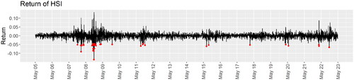
We first set up the period that is regarded as turbulence. In Figure 1, we mark with red dots the trading days that the return of HSI has dropped below three standard deviations from the mean over the whole study period. We find that it has covered most financial turbulence in the study period, including but not limited to the subprime mortgage crisis and the global financial crisis from mid-2007 to early 2009, the fluctuation from mid to late 2011, China’s stock market turbulence (Han and Khoojine 2019) from mid-2015 to early 2016, the trade war between the US and China (Liu 2018) in 2018, the COVID-19 pandemic in early 2020, and the rapid transmission of COVID-19 in Hong Kong and the continuation of warfare in Ukraine (Lockett 2022; Jiaxing Li 2022) in 2022. Therefore, we select the periods mentioned above as the turbulence.

Figure 1. Return of HSI. The red dots are the trading days that the return dropped below the three standard deviations from the mean over the whole study period.

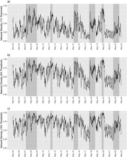
In Figure 2, we present the densities of $Y_{1\%}(t),$ $Y_{5\%}(t),$ and $Y_{10\%}(t),$ the time series of networks constructed using the critical values for a 21-day historical correlation to be significantly positive at the $1\%,$ $5\%$ and $10\%$ level, respectively. The regions shaded in gray are the periods when the financial turbulence occurs. We find that, except during 2022, when there is financial turbulence, the network densities often reach higher values than those during normal periods. The differences are more apparent in $Y_{1\%}(t)$ than in $Y_{5\%}(t)$ and $Y_{10\%}(t).$ The differences in network densities between the normal and turbulent periods allow us to recognize an early signal when we observe an unusual increase in network densities. This builds the foundation for our further analysis of the network and the embedded financial space.

Figure 2. The network densities over time of the three networks constructed using the critical value for a 21-day historical correlation to be significantly positive at the (a) $1\%,$ (b) $5\%,$ and (c) $10\%$ levels.

4.3. Properties of Our Proposed Measure in Financial Risk Management

We plot the results of the comparisons in Figure 3, in which each plot refers to a financial scenario comparing the specifications of the priors listed in Section 2.2. We summarize the four financial scenarios of interest in Table 2.

Figure 3. The systemic risk scores in four financial scenarios (Scenario 1: (a–c); Scenario 2: (d–f); Scenario 3: (g–i); Scenario 4: (j-l)) under three different threshold values of correlation in the construction of networks (1% Threshold: (a, d, g, j); 5% Threshold: (b, e, h, k); 10% Threshold: (c, f, i, l)). The red lines refer to the baseline systemic risk scores. The lines in other colors refer to the measurements of systemic risk under specific considerations.

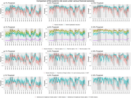
Table 2. The four financial scenarios that make use of the specifications of hyperparameters and distributions of choice are listed in Section 2.2.

Scenario	Specification of interest	Baseline
1	Allocation proportional to market capitalization	Random allocation
2	Allocation including a risk-free asset	Random allocation
3	Allocation with the industry of focus	Random allocation
4	Allocation with weights competition within groups	Allocation with equally shared industry sum of weights

The first specification represents a scenario that considers market capitalization, which equates to the total dollar value of a stock. A larger company often has a higher market capitalization and hence makes a greater contribution to systemic risk. Therefore, to calculate systemic risk, we use Dirichlet priors for the weights $\omega$ with the hyperparameters $\alpha$ proportional to the market capitalization shared among all stocks in the study; in other words, the prior mean is proportional to the market capitalization. To encourage the selection of weights that are close to the prior mean, we set the sum of all ${\alpha }_i$ to be the reciprocal of the smallest ${\alpha }_i,$ so that all entries of $\alpha$ are at least 1. This arrangement assigns a higher level of importance to those combinations of weights that follow the market capitalization closely. The sum of the hyperparameters controls the penalty on the level of importance for those weights deviating from the proportion of market capitalization. In Figure 3, the systemic risk score under the market capitalization allocation often has a higher systemic risk than the baseline. This is because approximately $70\%$ of the total market capitalization is shared by one-fourth of the stocks. Therefore, a change in log odds in any of the dominating stocks in the financial space produces a greater effect on the systemic risk score than on the baseline.

The second specification includes in the analysis a risk-free asset, which does not contribute to systemic risk. Therefore, to reduce the impact brought about by financial instability, we allocate a certain proportion of money to the risk-free asset. To measure the systemic risk encountered in the portfolio with different preferences for the proportions allocated to the risk-free asset, we assign hyperparameters corresponding to each preference. First, we set the hyperparameters ${\alpha }_i=1$ for all risky assets $i=1,\dots ,n.$ This provides a fair ground for comparison with the baseline, which always has zero weight assigned to the risk-free asset. We then consider three cases, with each taking a different hyperparameter for the risk-free asset ${\alpha }_{n+1}=1,10,100.$ The higher the hyperparameter for the risk-free asset, the higher the average proportion allocated to it. In our study, because the number of stocks varies over time, the corresponding average proportion allocated to the risk-free asset is also dynamic. Using the number of stocks that constitute the HSI on May 2023 – that is, $n=76$ – when ${\alpha }_{n+1}=1,10,$ and 100, the mean weights for the risk-free asset are $1.2987\%,$ $11.6279\%,$ and $56.8182\%,$ respectively. In Figure 3, the higher the hyperparameter that is assigned to the risk-free asset, the smaller the systemic risk is, and the gap between cases is wider during financial turbulence than during normal periods. Moreover, none of the four lines cross each other. Therefore, we can claim that increasing the allocation to a risk-free asset always decreases the effect of financial turbulence on the portfolio, especially during financial turbulence. Thus, practitioners could design their portfolios by changing the proportion allocated to risk-free assets, to monitor the systemic risk encountered in their investments.

The third specification assigns a fixed-weight sum of stocks in each industry. We demonstrate this with a focus on the Utilities industry to study the impact of the COVID-19 pandemic and the global energy crisis (Rankin et al. 2021). In our study, stocks are classified in $G=4$ industries. Therefore, the sum of weights for the Utilities industry is 0.5, while for all other industries the fixed sum of weights is equally shared, i.e. $0.5/3\approx 16.67\%$ for each of the remaining three industries. Using the stock classification by HSI on May 2023, there are five stocks from the energy industry, so their average weights are $0.5/5=10\%.$ This specification shows the systemic risk of the Utilities industry; maintaining half of the weights from other industries accounts for the impact outside the Utilities industry. We observe that before March 2020, the systemic risk of the energy industry is more or less close to the baseline, but after March 2020, the systemic risk is usually above the baseline. This observation matches the actual situation, in which the COVID-19 pandemic and the global energy crisis increased systemic risk in the Utilities industry.

The last specification also presets a sum of the weights of stocks in each industry. We allocate assets to the stocks equally in each industry, but we prefer only a few within each industry. In traditional portfolio theory, investing in a wider variety of stocks diversifies risk. In this specification, each industry shares the same preset sum of weights. However, amateur investors often do not allocate their money equally to all stocks and instead select only a few from each industry. Although the average weight is identical to both the specification of interest and the baseline, we find that the systemic risk score for the specification of interest generally is higher than the baseline. This coincides with conventional wisdom, as each relationship between companies becomes more important.

4.4. Comparisons of Our Proposed Measures with Alternative Formulations

We also compare the performance on raising an early signal by the systemic risk scores and other systemic risk measures in the literature. We again use the market capitalization allocation for the weights. We show the point-to-point comparison plot produced by dynamic time wrapping for each of the formulations of the same systemic risk scores and some common systemic risk measures that are listed in Appendix A.

To facilitate the discussion, we let $S_{1\%}(t),$ $S_{5\%}(t),$ and $S_{10\%}(t)$ be the time series of the systemic risk score constructed using the methods in Equation (14)(14) $$S(\omega ,C({\widehat{\eta }}_t))=\sqrt{{\omega }^{\top }C({\widehat{\eta }}_t)\omega },$$(14) , where the corresponding adjacency matrices of the input time series of the networks to estimate $\widehat{\eta }$ are $Y_{1\%}(t),$ $Y_{5\%}(t),$ and $Y_{10\%}(t)$ respectively. Let $S_{\mathit{\text{Das}},1\%}(t),$ $S_{\mathit{\text{Das}},5\%}(t),$ and $S_{\mathit{\text{Das}},10\%}(t)$ be the time series of systemic risk score constructed using the methods in Equation (A2)(A2) $$\begin{array}{cc}=\hfill & \sqrt{\sum _{i=1}^n\sum _{j=1}^n{y}_{i,j}{\omega }_i{\omega }_j},\hfill \end{array}$$(A2) , where the adjacency matrices to compute the systemic risk score on trading day t are $Y_{1\%}(t),$ $Y_{5\%}(t),$ and $Y_{10\%}(t)$ respectively. Let $S_{\mathit{\text{RE}},1\%}(t),$ $S_{\mathit{\text{RE}},5\%}(t),$ and $S_{\mathit{\text{RE}},10\%}(t)$ be the time series of the systemic risk score constructed using the methods in Equation (A5)(A5) $$\begin{array}{cc}=\hfill & \sqrt{\sum _{i=1}^n\sum _{j=1}^n{c}_{i,j}({\widehat{\eta }}^{{}^{\prime }}){\omega }_i{\omega }_j},\hfill \end{array}$$(A5) , where the input time series of networks to obtain estimated log odds are $Y_{1\%}(t),$ $Y_{5\%}(t),$ and $Y_{10\%}(t)$ respectively.

In Figure 4, the systemic risk measures and the returns in the HSI are in red and blue, respectively. Each dotted line links two points so that there is one from each time series. The color of the dotted line indicates the leading time series. The gray dotted line indicates a tie. We evaluate the performance of each systemic risk measure by observing the period preceding the turbulence, where the periods of turbulence are shaded in gray. The red dotted line between the two curves indicates that the systemic risk measure has shown a pattern that later appears in the HSI returns.

Figure 4. We compare by dynamic time wrapping the performance of the Das (2016) and our proposed systemic risk scores (red): using the financial space model (a–c), using the adjacency matrix directly (d–f), and using a random effects model (g–i), with the returns of the HSI (blue) as the reference. We construct the network using the critical value for 21-day of historical correlation to be significantly positive at the (a, d, g) $1\%,$ (b, e, h) $5\%,$ and (c, f, i) $10\%$ levels. We only present those dotted lines that are relevant to financial turbulence, to indicate the lead and lag relationships during the turbulence.

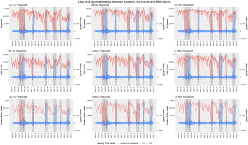
Figure 4 shows that regardless of the choice of systemic risk contribution and the threshold level in the construction of the network, we observe that there is an unusual climb in the values of the systemic risk score on or before the market crashes. Then, the systemic risk score falls gradually and keeps fluctuating until the next market crash.

Figure 4 also shows the performance of the systemic risk score in detecting an early signal of financial instability. To better illustrate, we have selected parts of the wrapping curve (dotted lines in the figures) that are relevant to the market crashes. We first observe the results from the network with the financial space. Before the global financial crisis in mid-2007, both the $S_{1\%}(t)$ and $S_{10\%}(t)$ lead the market return for 6 months during the crisis and continued to increase for 3 to 6 months throughout the crisis period. We believe with the 1% and 10% threshold, the systemic risk score successfully represents an early signal about the market. In the market crash brought on by the COVID-19 pandemic, the $S_{5\%}(t)$ and $S_{10\%}(t)$ value leads the market return for 3 months, while only the $S_{1\%}(t)$ values lead for 6 months. In $S_{1\%}(t),$ the number of days ahead of the crashes brought on by the COVID-19 pandemic is also too long to claim as an early signal. The $S_{5\%}(t)$ and $S_{10\%}(t)$ values continued leading for three months during the crisis, and the systemic risk score is also climbing during the crisis period. Therefore, we believe that an early signal is demonstrated successfully.

On the other hand, in the market turbulence from mid to late 2011, the systemic risk score failed to raise an early signal. All three systemic risk scores were lagging behind the market return. In the crashes from mid-2015 through early 2016, the systemic risk score also failed to raise an early signal. Although all of them lead the market before the crashes, the number of days ahead of the crashes in all the three $S_{1\%}(t),$ $S_{5\%}(t),$ and $S_{10\%}(t)$ are also too long to claim it as an early signal. Moreover, the climbing trend comes too late to raise an early signal. In the market turbulence in 2018, not to mention the lagging $S_{5\%}(t),$ although all of the $S_{1\%}(t)$ and $S_{10\%}(t)$ lead the market return, the number of days ahead are too long. Therefore, no early signal appears. Finally, in the market crash in 2022, none of the $S_{1\%}(t),$ $S_{5\%}(t)$ and $S_{10\%}(t)$ leads the market returns throughout the period. Although we observed a climb near the end of March, the systemic risk score has already missed the greatest drop in that period. Therefore, early signals also do not appear.

Different results are delivered when we use the adjacency matrix instead of the financial space to measure the contributions to systemic risk, i.e. the formulation proposed by Das (2016). As is shown in the middle row of Figure 4, during the global financial crisis from mid-2007 to early 2009, the systemic risk score does not lead the market return throughout the crisis for all the $S_{\mathit{\text{Das}},1\%}(t),$ $S_{\mathit{\text{Das}},5\%}(t),$ and $S_{\mathit{\text{Das}},10\%}(t).$ During the crashes brought by the COVID-19 pandemic, only the $S_{\mathit{\text{Das}},10\%}(t)$ leads for three months, giving a warning signal for the crisis, and in the remaining crashes, the systemic risk score lags the market returns. The leading by the $S_{\mathit{\text{Das}},5\%}(t)$ does not hold throughout the whole period of the COVID-19 pandemic crash. The $S_{\mathit{\text{Das}},1\%}(t)$ lags the market returns. In the market turbulence in mid to late 2011, the $S_{\mathit{\text{Das}},10\%}(t)$ has raised an early signal as it has led the market for 2 to 3 months. However, the leadership does not hold in $S_{\mathit{\text{Das}},1\%}(t)$ and $S_{\mathit{\text{Das}},5\%}(t).$ During the crashes in mid-2015 through early 2016, both $S_{\mathit{\text{Das}},5\%}(t)$ and $S_{\mathit{\text{Das}},10\%}(t)$ lead the market return, but the number of days ahead of the crashes is either too short or too long to claim it as an early signal. Moreover, the climbing trend in $S_{\mathit{\text{Das}},10\%}(t)$ comes too late to raise an early signal. None of $S_{\mathit{\text{Das}},1\%}(t),$ $S_{\mathit{\text{Das}},5\%}(t),$ and $S_{\mathit{\text{Das}},10\%}(t)$ lead the market throughout the whole crashes in 2018 and 2022.

Similar observations were found when we used the random effects model to measure the contribution to systemic risk. The systemic risk score led the market returns during the global financial crisis from mid-2007 to early 2009 only in $S_{\mathit{\text{RE}},1\%}(t)$ and $S_{\mathit{\text{RE}},5\%}(t),$ and the leadership with the $S_{\mathit{\text{RE}},10\%}(t)$ does not persist throughout the whole period. For the market crash brought by the COVID-19 pandemic, only the $S_{\mathit{\text{RE}},10\%}(t)$ leads for three months, giving a warning signal for the crisis. In the market turbulence from mid to late 2011, all the $S_{\mathit{\text{RE}},1\%}(t),$ $S_{\mathit{\text{RE}},5\%}(t),$ and $S_{\mathit{\text{RE}},10\%}(t)$ failed to lead the market throughout the whole period. In the market crash from mid-2015 through early 2016, the $S_{\mathit{\text{RE}},5\%}(t)$ and $S_{\mathit{\text{RE}},10\%}(t)$ thresholds lead for 6 months. However, it is hard to claim that as a warning signal because the value of systemic risk is moving downward. In other combinations of thresholds and crashes, the systemic risk scores lag the market returns. In the turbulence throughout 2018, $S_{\mathit{\text{RE}},1\%}(t)$ lags the market return. Even though $S_{\mathit{\text{RE}},5\%}(t)$ leads the market return in the market, the systemic risk score is declining in the pre-crisis period and not lead throughout the whole period. The $S_{\mathit{\text{RE}},10\%}(t)$ also suffers from a similar issue but lags the market return in most of the turbulence period.

We also compare the number of times that the systemic risk score leads the market returns with reference to Figure 5 and Table 3. The proposed systemic risk score has a similar number of time points that leading the returns of the HSI when comparing them with the scores using the adjacency matrix and the random effects models. Comparing the systemic risk score based on the $Y_{1\%}(t),$ the proportion of time that the $S_{1\%}(t)$ leads the market returns is larger than $S_{\mathit{\text{RE}},1\%}(t),$ followed by $S_{\mathit{\text{Das}},1\%}(t).$ Comparing the systemic risk score based on the $Y_{5\%}(t),$ the proportion of time that the $S_{5\%}(t)$ leads the market returns is smaller than both $S_{\mathit{\text{RE}},5\%}(t),$and $S_{\mathit{\text{Das}},5\%}(t).$ Finally, comparing the systemic risk score based on the $Y_{10\%}(t),$ the proportion of time that $S_{\mathit{\text{RE}},10\%}(t)$ leads the market returns is the least, followed by the $S_{10\%}(t),$ and finally the $S_{\mathit{\text{Das}},10\%}(t).$ We believe that it is more important to lead the market returns, as an early signal, in the proximity of the crashes. Therefore, in terms of the early signal that we have successfully demonstrated, the systemic risk score based in the financial space performs better than the other two setups do.

Figure 5. The complete wrapping curves between the Das (2016) and our proposed systemic risk scores (red): using the financial space model (a-c), using the adjacency matrix directly (d-f), and using a random effects model (g-i), with the returns of the HSI (blue) as the reference. We construct the network using the critical value for 21-day of historical correlation to be significantly positive at the $1\%$ (a, d, g), $5\%$ (b, e, h), and $10\%$ levels (c, f, i).

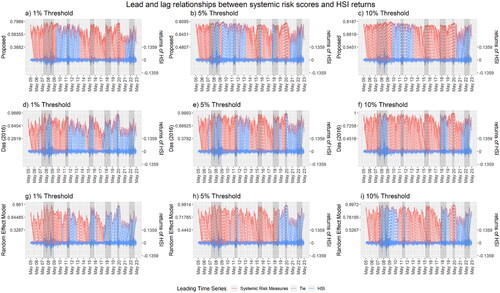
Table 3. Number of time points in the wrapping curve that each systemic risk score leads, ties with, or lags the returns of the HSI, as summarized from Figure 5.

	Number of time points (in percentage)
Systemic risk Score	Leading the returns of the HSI	Tying the returns of the HSI	Lagging the returns of the HSI
$S_{1\%}(t)$	2984	3	1450
	(67.2526 %)	(0.0676 %)	(32.6797 %)
$S_{5\%}(t)$	2461	23	1953
	(55.4654 %)	(0.5184 %)	(44.0162 %)
$S_{10\%}(t)$	3020	15	1402
	(68.064 %)	(0.3381 %)	(31.5979 %)
$S_{\mathit{\text{Das}},1\%}(t)$	1770	26	2641
	(39.8918 %)	(0.586 %)	(59.5222 %)
$S_{\mathit{\text{Das}},5\%}(t)$	2496	28	1913
	(56.2542 %)	(0.6311 %)	(43.1147 %)
$S_{\mathit{\text{Das}},10\%}(t)$	3394	13	1030
	(76.4931 %)	(0.293 %)	(23.2139 %)
$S_{\mathit{\text{RE}},1\%}(t)$	2405	16	2016
	(54.2033 %)	(0.3606 %)	(45.4361 %)
$S_{\mathit{\text{RE}},5\%}(t)$	3269	14	1154
	(73.6759 %)	(0.3155 %)	(26.0086 %)
$S_{\mathit{\text{RE}},10\%}(t)$	2677	17	1743
	(60.3336 %)	(0.3831 %)	(39.2833 %)

Next, we consider the performance of other systemic risk measures. Figure 6 shows the performance of three other systemic risk measures in providing an early signal of financial instability. Again, those regions shaded in gray are the periods of market turbulence or worldwide financial incident. We have selected the parts of the wrapping curve that are relevant to the market crashes for better illustration.

Figure 6. We compare here by dynamic time wrapping the performances of three other systemic risk measures: (a) $\Delta$ CoVaR, (b) the systemic expected shortfall, and (c) the absorption ratio, using the returns of the HSI as the reference time series. We include only the dotted lines for the time points that are relevant to financial turbulence.

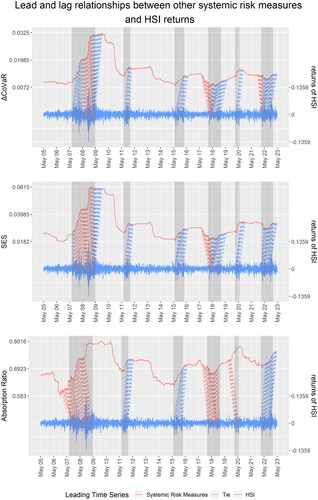
Although all three measures climb during most market crashes, the systemic risk measure seldom leads the market returns throughout the periods of the crashes. Among all of the other systemic risk measures considered in this study, only the absorption ratio (AR), defined in Appendix A.5, leads the market returns during the global financial crisis from mid-2007 to early 2009, the turbulence throughout 2018, and also during the crash of the COVID-19 pandemic, for 6 to 9 months. However, as an early signal, the AR may not be dependable given the low position of the value of the AR before the global financial crisis from mid-2007 to early 2009. It is even dropping before the turbulence throughout 2018. The only time that we can claim the AR as an early signal is before the COVID-19 pandemic, when the AR keeps climbing, especially with a jump after late 2019, until mid-2020.

In the global financial crisis from mid-2007 through early 2009, $\Delta$ CoVaR leads only from mid-2008 to early 2009, which covers the strongest period of the crash throughout the study period. However, the measure lags during the remaining period of the crisis. The Systemic Expected Shortfall (SES), defined in Appendix A.4, leads from mid-2007 to early 2009 but still does not lead throughout the whole financial crisis, and it also lags the market returns in the most remaining market crashes.

5. Discussion

In this paper, we have proposed a new approach for predicting systemic financial risk by using stock return correlations, financial networks, and a latent unobserved financial space. We first observe the relationships between institutions through the correlations among their stock returns, demonstrating that the stock returns often reveal the impact of news about an institution. If two institutions have a significant relationship, any impact on one could transfer to the other institution, so by capturing the correlations among their stock returns, we can evaluate the strength of the relationship between the two institutions.

In the business world, institutions can be related either directly or indirectly. Where there is a direct relationship, institutions may rely on each other to earn revenue, and the failure of one can severely harm others’ ability to earn. In the case of an indirect relationship, the contagion of failure from one institution to others can occur between other institutions that do not have a direct relationship with the source of failure. The key issue, therefore, is how strongly two institutions are related, rather than whether or not any relationship between them exists. A failure in one institution that has a strong relationship with others can lead to subsequent failures in the other institutions, and we therefore construct a financial network to use for capturing those strong inter-institutional relationships. That financial network shows that relationships are stronger during financial turbulence than in normal periods.

To better explain the contagion of systemic risk, we have introduced the concept of financial space, which is closely related to the visualization of network and latent space modeling. We allow each institution to take its optimal position in the financial space so that the distances between institutions accurately reflect their relationships. At the same time, the financial space allows us to visualize the relationship by embedding the financial space into the network. The position of stocks in the financial space represents the market situation in the sense the denser the financial space, the greater the systemic risk.

We thus make use of the distances between institutions in the financial space as one of the inputs to our proposed systemic risk score. A previous study took the network itself into account (Das 2016) that we base on their work. First, we dynamically relate the systemic risks together. Often the relationships between companies are time-dependent, and the financial space model has the potential to keep track of changes in those relationships and to give an early warning signal of upcoming financial instabilities via the model’s systemic risk scores. The second advancement is that we smooth the systemic risk score by replacing the binary value in the adjacency matrix with the distance between the stocks in the network plot. This gives more information about the closeness of the relationship between each pair of companies. The third advancement is the use of Bayesian decision setting, which allows for consideration of various financial situations. Our systemic risk scores take the weights assigned to each stock as the second input. Often, a particular setting of a stock’s weight is insufficient to describe a financial situation, but in using the Bayesian decision theory we collect all possible cases and give each a level of importance according to how well each case fits the financial situation. We believe this provides a better picture with which investors and portfolio managers can monitor systemic risk in their situations.

In our study, we have also compared the performance of the systemic risk score with various other systemic risk measures from previous studies. We have used the dynamic time wrapping technique to match the pattern of the systemic risk measures and the returns of the Hong Kong market. Our proposed systemic risk score using the financial space fairly consistently leads the returns of the HSI beginning roughly three months before the historical worldwide financial incident, including the global financial crisis and the COVID-19 pandemic. Although our measure is not perfect in producing an early signal all of the time, the performance is better than that of other measures, including that using an adjacency matrix (Das 2016) and an institution-specified random effects model.

On the other hand, the indication of turbulence in a smaller scale incident, like those from mid to late 2011, from mid-2015 to early 2016, and throughout 2018 and 2022, is weaker than the indication in a worldwide financial incident. We believe that the worldwide financial incident is caused by the superposition of multiple factors. Before the crashes, the systemic risk score captures some of the factors and has sufficient time to raise a signal. Therefore, even though the performance of the systemic risk score on a smaller scale of the incident is not as satisfactory as in a worldwide financial incident, the climbing systemic risk score over the turbulence period can also be a sign of accumulating the factors to trigger a larger scale of the incident.

We have also demonstrated several applications of the systemic risk scores in the Bayesian framework. By assigning a suitable before the weights, we inject our beliefs into the measurement of systemic risk. Our score for systemic risk also has an intuitive explanation in accord with traditional knowledge in investment, so investors can apply their knowledge to determine the systemic risk in their investment. Once the contribution of systemic risk is determined, we can change our prior belief for various applications and recompute the systemic risk score without spending much computational power.

Our proposed approach for predicting systemic risk inherits the advantage from Das (2016) that the score is a general approach to studying systemic risk. We have chosen the correlation of stock returns as our source of data to construct the network. As we explain in Section 4.2, during financial turbulence, the networks of institutions are usually more connected than they are during normal periods. This is one of the criteria for being a good source of data for measuring the relationships’ contribution to the systemic risk score. However, because the correlations measure the institutional associations and do not consider the interactions, they might not be the perfect measure of connectedness. Nevertheless, as we discussed in Section 2.4, the latent space model can capture the relationships through a chain of intermediates, which is often neglected in network studies, and because the distances in the latent space are symmetric, they are natural for embedding an undirected network. Therefore, we decide to use an undirected network, and hence we have to set symmetric criteria, for the correlation, to determine whether a pair of stocks is linked.

Since we build both the financial space model and the random effect model based on whether there are edges between two nodes in the network, and summarize the estimated chance of observing a link via averaging, as shown in our study, the performance of the systemic risk score can be linked to network densities. On one hand, from Figure 2, we observe that before the turbulence from mid-2015 to early 2016, and throughout 2018, the network densities are dropping. On the other hand, we found a similar pattern in all sub-figures in Figure 6.

We also find that the systemic risk score in the turbulence period of 2022 is lower than other normal periods. The major reason is the absence of edges in the network. This means that there are fewer pairs of stocks having a significant correlation, which coincides with the result in Figure 2. However, the correlation of stock returns is not the only factor that triggers market turbulence. This is one example showing that the correlation measure is not a perfect criterion to determine the edge in the network.

Therefore, we suggest readers, who are interested in applying the model to other datasets, first examine the network densities, which require much less computation cost, for a glance at the limitation of the resulting systemic risk score with their data input. Nevertheless, it does not mean that the network densities have a similar performance as the financial space model or the random effect model. As the formulation of Das (2016) is solely based on the adjacency matrix, which gives a systemic risk score even more closely related to the network densities than those via models, we can see from Figure 6 that the systemic risk score using the network densities alone cannot make the same performance as those using the financial space model and the random effect model.

Moreover, our proposed systemic risk score is not confined to a single type of data—it is flexible enough to measure the systemic risk even if the contribution to systemic risk C is not symmetric. Therefore, a possible direction for future research is to determine and compare systemic risk scores using the contributions of systemic risk based on various sources of data. For example, in the study of the social network, we can use the proposed financial space concept to create a latent social space to detect social communities (Gerlach et al. 2018). The systemic risk score proposed in this study can be a measure of the strength of relationships within a community or a measure of social capital (Shin 2021). In epidemiological studies, a contagion space provides a latent plane to study the evolution of pandemic (So et al. 2020b; Chu et al. 2020, 2021). The proposed financial space can be interpreted as a pandemic space where the proposed systemic risk score can give a measure of pandemic risk. From the information retrieval perspective, our approach can help to analyze a dynamic news topic network (So et al. 2022) and a Google Trends dynamic network (Chu et al. 2023).

In addition, the network construction process converts a continuous measure into a binary one, and information about the strength of the relationship is lost. We can partially see the effect on loss when we compare the proposed systemic risk score with the systemic risk score using the adjacency matrix directly. A remedy would be to incorporate multiple levels together, such as the three levels of thresholds we used in our study. The levels would be sequential, so the correlations would be required to pass the lower level before they could reach a higher level. By doing that, we could reduce the loss of information in the conversion and could distinguish those institutions with stronger relationships.

Last, we find that the systemic risk scores fluctuate more vigorously than other systemic risk measures do, such as the SES, $\Delta$ CoVaR, and absorption ratio. We can also observe this feature in Figure 2, the network density plot. An advantage of this feature is that the systemic risk scores are more sensitive to the latest market situations. However, such fluctuations can also produce a false positive that initiates a false warning signal. We believe that by tuning the number of days of correlation to be considered in the formation of the network, we could strike a balance between the model’s sensitivity to market updates and the false positive issue.

Acknowledgements

We thank the Editor-in-Chief, Professor David Matteson, and four anonymous reviewers for their helpful comments. We also thank the Turing AI Computing Cloud (TACC) platform for providing us with the computational resources to conduct the analyses in this paper. This work was partially supported by the Hong Kong RGC Theme-based Research Scheme, grant number T31-604/18-N, and The Hong Kong University of Science and Technology research grant “Risk Analytics and Applications” (grant number SBMDF21BM07). The funding recipient was MKPS.

Disclosure statement

No potential conflict of interest was reported by the author(s).

Additional information

Funding

This work was supported by the Hong Kong University of Science and Technology [SBMDF21BM07], Research Grants Council, University Grants Committee [T31-604/18-N].

Appendix A.

Other Measures of Systemic Risk in the Literature

Several approaches have been used to create systemic risk measures in previous studies. In this study, we have compared the performance of our score with that of other measures. The first two are related to our score, one of which is the systemic risk score proposed by Das (2016), which uses the adjacency matrix of the network as the contribution of systemic risk, without accessing the financial space. The other one uses a random effects model instead of the financial space model. The remaining three are common systemic risk measures in the literature: $\Delta$ CoVaR, SES, and AR.

A.1 Using Adjacency Matrix of Network

The first approach, motivated by Das (2016), considers the adjacency matrix of the network as the contribution of systemic risk. Because the existence of an edge between nodes represents a significant relationship, we calculate the systemic risk by replacing the contribution of systemic risk C with $Y=(y_{i,j}),$ the adjacency matrix of the network linking the stocks with significant business relationships: (A1) $$S(\omega ,Y)=\sqrt{{\omega }^{\top }Y\omega }$$(A1) (A2) $$\begin{array}{cc}=\hfill & \sqrt{\sum _{i=1}^n\sum _{j=1}^n{y}_{i,j}{\omega }_i{\omega }_j},\hfill \end{array}$$(A2) where $\omega$ is the weight. The adjacency matrix contains only a binary value, which equals the sum of the products of weights of those institutions that have significant relationships. We have used this formulation in Section 4.4 to compare the systemic risk score under this setting to other formulations, showing the differences and advantages in using the financial space over solely considering the direct relationship between institutions in Figure 4.

A.2 Using Institution-Specified Random Effect Model

The second approach considers an institution-specified random effects model instead of the latent space model. In Section 2.3.4, the financial space affects the log odds via the distance between institutions in the space. We consider an alternative to replace the distance with a sum of two random effects, one on each institution of the pair under consideration. (A3) $${\eta }_{i,j,t}^{{}^{\prime }}=z_i^{{}^{\prime }}+z_j^{{}^{\prime }}+\sum _{m=1}^M{\beta }_m{X}_{i,j,t,m},$$(A3) where $z_i^{{}^{\prime }}$ and $z_j^{{}^{\prime }}$ are univariate random intercepts. This comparison assesses the performance of our proposed model versus that of a simpler standard base model. The apostrophe on $z_i^{{}^{\prime }}$ and $z_j^{{}^{\prime }}$ distinguish the random intercept from the latent position. Similarly, the apostrophe on ${\eta }_{i,j,t}^{{}^{\prime }}$ distinguishes the two formulations of log odds.

Let ${\widehat{\eta }}_{i,j,t}^{{}^{\prime }}$ be the estimated log odds using the random effects model specified by Equation (A3)(A3) $${\eta }_{i,j,t}^{{}^{\prime }}=z_i^{{}^{\prime }}+z_j^{{}^{\prime }}+\sum _{m=1}^M{\beta }_m{X}_{i,j,t,m},$$(A3) on a trading day t, and let ${\widehat{\eta }}^{{}^{\prime }}=({\widehat{\eta }}_{i,j,·}^{{}^{\prime }})$ be the matrix of the estimated log odds. We need to transform the estimated log odds to ensure that the contribution to systemic risk is positive. Again, the natural choice is Equation (13)(13) $$c_{i,j}\left({\widehat{\eta }}_t\right)=\frac{1}{1+\hspace{0.17em}\mathrm{\text{exp}}\hspace{0.17em}\left(-{\widehat{\eta }}_{i,j,t}\right)}$$(13) . We substitute $C({\widehat{\eta }}^{{}^{\prime }})$ into C to calculate the systemic risk: (A4) $$S(\omega ,f({\widehat{\eta }}^{{}^{\prime }}))=\sqrt{{\omega }^{\top }C({\widehat{\eta }}^{{}^{\prime }})\omega }$$(A4) (A5) $$\begin{array}{cc}=\hfill & \sqrt{\sum _{i=1}^n\sum _{j=1}^n{c}_{i,j}({\widehat{\eta }}^{{}^{\prime }}){\omega }_i{\omega }_j},\hfill \end{array}$$(A5) where $\omega$ is the weight. The random effects model is a simplified model of our latent space model. We have used this formulation in Section 4.4 to compare the systemic risk score under this setting to the one using financial space, showing the ability to capture the indirect business relationship with the financial space in Figure 4.

A.3 Using $\Delta$ CoVaR

The third approach measures the change of conditional value-at-risk (CoVaR) in the market returns when there is distress on stock j from the CoVaR of market returns when stock j is of normal status. In other words, it is the difference between the market returns when the return of stock j equals its VaR and when the return of stock j equals its median.

In our study, we define the distress as $5\%$ VaR, which is defined by the $5^{\mathit{\text{th}}}$ percentile of the returns of stock within the most recent two years. Some stocks have incomplete information within the last two years, which may be due to non-listing or other reasons. We first let ${\mathcal{I}}_t$ be the set of stocks with no missing returns within the last two years preceding the trading day t. We denote the number of stocks in ${\mathcal{I}}_t$ by $N_t.$ On trading day t, we let $\mathit{\text{Va}}{R}_j^q(t)$ be the $q\%$ VaR of stock j. In particular, when $q=50,$ we have $\mathit{\text{Va}}{R}_j^{50}(t)$ as the median of the returns of stock j. We replace the subscript j with market when we are referring to the market returns. Furthermore, we denote $\mathit{\text{CoVa}}{R}_{\mathit{\text{market}}|j}^q(t)$ to be the $q\%$ VaR of the market, given that the return of stock j is $\mathit{\text{Va}}{R}_j^q(t).$ Therefore, the value of $\mathit{\text{Va}}{R}_j^q(t)$ and $\mathit{\text{CoVa}}{R}_{\mathit{\text{market}}|j}^q(t)$ satisfy the following equations, with respect to the returns in the last two years preceding trading day t: (A6) $$P(r_{j,t}\le \mathit{\text{Va}}{R}_j^q(t))=q/100,$$(A6) (A7) $$\begin{array}{cc}P(r_{\mathit{\text{market}},t}\le \mathit{\text{CoVa}}{R}_{\mathit{\text{market}}|j}^q(t)|r_{j,t}=\mathit{\text{Va}}{R}_j^q(t))\hfill & =q/100,\hfill \end{array}$$(A7) where $r_{\mathit{\text{market}},t}$ is the market returns at trading day t, and we use $q=5$ and 50 for our study.

We measure the systemic risk of the market on trading day t by taking an average of (A8) $$\Delta \mathit{\text{CoVa}}{R}_{\mathit{\text{market}}|j}^5(t):=\mathit{\text{CoVa}}{R}_{\mathit{\text{market}}|j}^{50}(t)-\mathit{\text{CoVa}}{R}_{\mathit{\text{market}}|j}^5(t)$$(A8) over all j.

A.4 Using the Systemic Expected Shortfall

The fourth approach considers the distress over the whole market rather than that of a particular stock. We let $\mathit{\text{Va}}{R}_{\mathit{\text{market}}}^q(t)$ to be the $q\%$ VaR of the market on trading day t, and $E_{j|\mathit{\text{market}}}^q(t)$ be the expected return of stock j conditional on the market return on the trading day t less than ${\mathit{\text{Var}}}_{\mathit{\text{market}}}^q(t).$ Then, $E_{j|\mathit{\text{market}}}^q(t)$ satisfies the following equation, with respect to the returns in the most recent two years. (A9) $$E_{j|\mathit{\text{market}}}^q(t)=|A_{t,q}{|}^{-1}\sum _{t\in A_{t,q}}{r}_{j,t},$$(A9) where $A_{t,q}$ is the collection of trading days of size $\left|A_{t,q}\right|$ in the last two years before the trading day t, so that the market return is less than ${\mathit{\text{Var}}}_{\mathit{\text{market}}}^q(t).$ In other words, trading day $t^{\prime }$ is inside $A_{t,q}$ if $r_{\mathit{\text{market}},t^{\prime }}\le \mathit{\text{Va}}{R}_{\mathit{\text{market}}}^q(t^{\prime })$ and the trading day $t^{\prime }$ is in the last two years preceding trading day t. We measure the systemic risk of the market on trading day t by taking the average of $E_j(t)-E_{j|\mathit{\text{market}}}^q(t)$ over all j with $q=5.$ (A10) $$\mathit{\text{SES}}(t)=\frac{1}{N_t}\sum _{j\in {\mathcal{I}}_t}{E}_j(t)-E_{j|\mathit{\text{market}}}^5(t),$$(A10) where $E_j(t)$ is the (unconditional) expected returns of stock j.

A.5 Using Absorption Ratio

The last approach we analyzed from previous studies considers the proportion of information absorbed by the first few principal components in the two-year historical covariance matrix of stock returns. That covariance matrix provides information on the variation in stock returns that cannot be explained by the average returns. The principal components analysis sequentially extracts the most important information from the covariance matrix while ensuring that there are no correlations in the information. If the first few principal components can explain most of the information in the covariance matrix, the variation most likely depends on these pieces of information. In other words, these few pieces of information control the variation of the stocks. If this important information is adverse news, it drives the stock returns to fall together, and that creates an impact on the market.

We study the proportion of information absorbed by the first $\lfloor N_t/5\rfloor$ principal components of the historical covariance matrix ${\Sigma }_t$ of stock returns in the last two years preceding trading day t. If the returns are available for all 76 stocks constituting the Hang Seng Indexes in May 2023, we consider the first 15 principal components (rounded down to the nearest integer). Let ${\lambda }_{1,t}>{\lambda }_{2,t}>\dots >{\lambda }_{N_t,t}>0$ be the eigenvalues and let $v_{1,t},v_{2,t},\dots ,v_{N_t,t}$ be the corresponding eigenvectors of ${\Sigma }_t.$ We then have the following equation satisfied, (A11) $${\Sigma }_t{v}_{i,t}={\lambda }_{i,t}{v}_{i,t}.$$(A11)

Therefore, we calculate the absorption ratio by (A12) $$\mathit{\text{AR}}(t)=\frac{\sum _j^{\lfloor N_t/5\rfloor }{\lambda }_{j,t}}{\sum _{j^{\prime }}^{N_t}{\lambda }_{j^{\prime },t}}.$$(A12)

Appendix B.

Dynamic Time Wrapping

Suppose that two time series have T trading days. A wrapping curve $\varphi (k)=({\varphi }_S(k){\varphi }_R(k))$ is a function taking value value from $\{1,\dots ,K\}$ as input and returning value from $\{1,\dots ,T\}\times \{1,\dots ,T\}$ as output, pairing K points from each of the time series and satisfying the following requirements:

1. ${\varphi }_S(1)={\varphi }_R(1)=1,$

2. ${\varphi }_S(K)={\varphi }_R(K)=T,$

3. ${\varphi }_S(k+1)\ge {\varphi }_S(k)$ and ${\varphi }_R(k+1)\ge {\varphi }_R(k).$

These requirements align the starting and ending points of both time series, and ensure that the wrapping curve matches points along the time. Moreover, the wrapping curve has to follow the local slope constraints, so that the ${\varphi }_S(k+1)-{\varphi }_S(k)$ and ${\varphi }_R(k+1)-{\varphi }_R(k)$ are restricted according to the step pattern (Tormene et al. 2009). We will introduce the step pattern of interest in a later paragraph.

The dynamic time wrapping algorithm aims at an optimal wrapping curve $\varphi$ so that the average accumulated distortion between $S({\varphi }_S(k))$ and $R({\varphi }_R(k))$ is minimized. The distortion refers to the extent of mismatch in the two time series. The first factor is the absolute difference between the two time series S and R at trading days $t^{\prime }$ and $t^{″}$ as the distortion. (B1) $$\mathcal{D}(t^{\prime },t^{″})=|S(t^{\prime })-R(t^{″})|.$$(B1)

The second factor depends on the step pattern together with a normalizing constant. Therefore, given $\varphi (k),$ among all possible choices of $\varphi (k+1),$ the step pattern also takes part in determining the optimal wrapping curve. The normalization constant makes sure the wrapping curve $\varphi$ of different lengths is comparable. Joining all of the information together, the average accumulated distortion is defined. (B2) $${\mathcal{D}}_{\varphi }(S,R):=\sum _{k=1}^K\mathcal{D}({\varphi }_S(k),{\varphi }_R(k))m_{\varphi }(k)/M_{\varphi },$$(B2) where $m_{\varphi }(k)$ is a per-step weighting coefficient and $M_{\varphi }$ is the corresponding normalization constant to make sure the wrapping curves $\varphi$ with different lengths are comparable.

Because the first factor of distortion is measured in an absolute sense, both the location and scale of the time series have an impact on the resulting wrapping curve (Giao and Anh 2016). Therefore, a suitable transformation is necessary for a meaningful result. In our study, we have chosen the z standardization, translating and scaling the whole time series so that the mean and the standard deviation of the resulting time series are 0 and 1, respectively. The market return has been further multiplied by negative 1 so that a spike in the systemic risk score matches a crash in the market return.

In the above constraints on the wrapping curve, the alignment of the starting and ending points may produce a bias in studying the lead and lag relationships. Therefore, we follow Tormene et al. (2009) to allow open start and end points, and we make further assumptions as a replacement to achieve a meaningful wrapping curve:

1. ${\varphi }_S(k)=k,$

2. ${\varphi }_R(k+1)-{\varphi }_R(k)$ is either 0, 1, or 2, and

3. $|{\varphi }_S(k)-{\varphi }_R(k)|\le 150.$

The first constraint fixes the function ${\varphi }_S(k)$ and the value of K to be T. The third constraint bounds the points in the two time series to match a moderate integer (Sakoe and Chiba 1978), which here we have chosen to be 150. The first two constraints constitute the so-called asymmetric step pattern, so that $m_{\varphi }(k)=1$ and $M_{\varphi }=N.$

Appendix C.

Computational Details Related to the Proposed Systemic Risk Score

First, to facilitate the computation of the systemic risk score, no matter which distribution is assigned to the weights, we use a simulation-based approach to calculate the systemic risk score. In our study, we simulate a sample of size $L=1000$ and estimate the systemic risk score by (C1) $$S(·)=\frac{1}{L}\sum _{l=1}^{L}S({\omega }^{(l)},C),$$(C1) where ${\omega }^{(l)}$ is simulated from the distribution of weights, and C is the contribution to systemic risk.

Referring to Section 2.2, we have considered two choices of priors in our study. The first one is a Dirichlet distribution. The sampling procedure is standard. The second choice requires sampling from a Dirichlet distribution multiple times. Suppose we have fixed G, which is the number of groups in total, and have determined the sum of weights ${\omega }_{(g)}^{+}$ in each group. For each group g, we sample ${\omega }_{(g)}$ from the Dirichlet distribution of the dimension being the number of stocks in group g. Then, we concatenate all ${\omega }_{(g)}/{\omega }_{(g)}^{+}$ together to form $\omega ,$ a vector of length n, so that the sum of all entries in $\omega$ equals 1.

Appendix D.

Diagnostic of the MCMC Estimation

In our experiment, we employ $Q+1=11$ particles in the particle Gibbs with ancestor sampling approach. Additionally, we conduct a separate experiment using $Q+1=51$ particles to examine the impact on the MCMC diagnostics. Thus, in this section, we present the MCMC diagnostic results for both settings.

D.1 Posterior Plot

Figure D1 shows the log of the posterior density of every iteration in each rolling sample. Figure D1 shows that the Markov chains in each rolling sample have converged after the burn-in. Comparing both sides of the figures, the log of posterior density does not show much difference when using $Q+1=11$ and $Q+1=51$ particles.

D.2 Trace plot of Selected Parameters

Figure D2 and D3 display the trace plots of selected parameters in each rolling sample for $Q+1=11$ particles and $Q+1=51$ particles, respectively. Both figures demonstrate that the parameters in each rolling sample have converged after the burn-in period. We have also selected some parameters related to the financial space, but we defer the demonstration and the discussion of these parameters to Appendix E.

D.3 Step size Adaptation and Acceptance Rate

As described in Section 3.6, we adjust the step size during the burn-in period to achieve an optimal acceptance rate. Table D1 provides a summary of the average finalized step size for each parameter and systemic risk score using $Q+1=11$ and $Q+1=51$ particles, respectively. The step size for $z_{i,t}$ is automatically tuned by the particle Gibbs with ancestor sampling scheme, as explained in Section 3.5. The average step sizes for $\mu ,$ $\Gamma ,$ and $\tau$ across all stocks and dimensions are reported.

Table D2 and D3 shows the minimum, mean, and maximum of the average acceptance rates over all parameters, excluding $\mathcal{Z},$ during each MCMC stage and of each systemic risk score when using $Q+1=11$ and $Q+1=51$ particles respectively. After the burn-in period, in both $Q+1=11$ and $Q+1=51$ particles, the mean of the average acceptance rate stays at or slightly above the upper bound of the desired intervals, i.e. 0.268.

Figure D4 illustrates the update rate of the particle Gibbs approach applied to the financial space $\mathcal{Z}$ for three selected rolling samples (i.e. rolling samples 4, 118, and 216). The update rate of $z_{i,t}$ represents the proportion of iterations in which the value of $z_{i,t}$ changes. We observe that, in general, using a higher threshold percentage on the networks and a larger number of particles results in a higher update rate.

While the update rates typically range from 0.8 to 0.85 for $Q+1=11$ particles and around 0.95 for $Q+1=51$ particles on most trading days, occasional drops below these levels are inevitable due to particle degeneracy (Chopin and Singh 2015). However, it does not show a pattern of increasing update rates from a low value at the beginning. Instead, the rates fluctuate around a level slightly lower than the ideal rate Lindsten et al. (2014). We believe that the use of ancestor sampling has mitigated the issue of particle degeneracy.

D.4 Effective sample size

We calculate the effective sample size using the coda package in R (Plummer et al. 2006). Table D4 and D5 present the minimum, mean, and maximum average effective sample sizes across parameters during the burn-in period, after the burn-in period, and the entire MCMC period using $Q+1=11$ and $Q+1=51$ particles, respectively. Occasionally, the dependence among model parameters results in a lower effective sample size, but in general, the effective sample size reaches around 1500. Additionally, we observed that the effective sample size does not differ much between $Q+1=11$ and $Q+1=51$ particles.

D.5 Area under ROC

To assess the accuracy of our model in estimating the edges in the network, we compute and illustrate in Figure D5 the area under the receiver operating characteristic (AUROC) curve for each rolling sample and each network threshold $Y_{1\%}(t),$ $Y_{5\%}(t),$ and $Y_{10\%}(t)$ using $Q+1=11$ and $Q+1=51$ particles. We observe that a smaller threshold percentage yields a higher accuracy. Furthermore, there is an improvement in AUROC when using $Q+1=51$ particles compared to $Q+1=11$ particles.

D.6 Computation Time

In the rolling sample analysis, the number of stocks n and the number of trading days T vary. The number of stocks n ranges from 28 to 65, corresponding to the number of constituents in HSI. The number of trading days T ranges from 487 to 501. To indicate how well the algorithm scales, we selected three sets of n and T (i.e. rolling samples 4, 118, and 216) and reported the computation time in Table D6. We believe that the computation time grows linearly with n. However, since the variation in T in the rolling sample analysis is small, it is difficult to determine precisely how the computation time grows with T. When comparing the computation time between $Q+1=11$ and $Q+1=51$ particles, we believe that the computation time grows linearly with Q.

Figure D1. The posterior plot of each rolling sample (arranged in colors) for all three thresholds (1% Threshold: (a-b); 5% Threshold: (c-d); 10% Threshold: (e-f)) along the iterations using $Q+1=11$ (a, c, e) and $Q+1=51$ (b, d, f) particles.

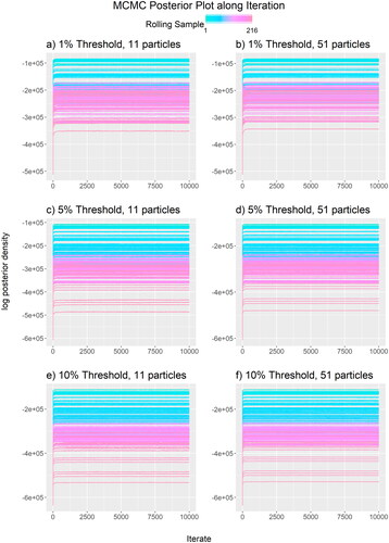
Figure D2. The trace plot of effect parameters in each rolling sample (arranged in colors) for all three thresholds (1% Threshold: (a, d, g, j); 5% Threshold: (b, e, h, k); 10% Threshold: (c, f, i, l)) along the iterations when using $Q+1=11$ particles.

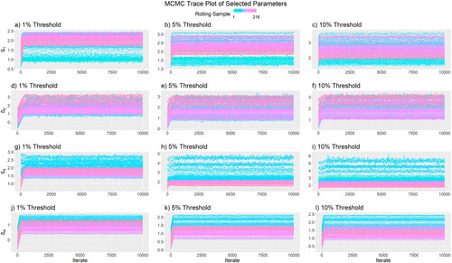
Figure D3. The trace plot of effect parameters in each rolling sample (arranged in colors) for all three thresholds (1% Threshold: (a, d, g, j); 5% Threshold: (b, e, h, k); 10% Threshold: (c, f, i, l)) along the iterations when using $Q+1=51$ particles.

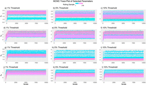
Figure D4. The update rate of the particles Gibbs approach with $Q+1=11$ (solid) and $Q+1=51$ particles (dashed) to the parameter $\mathcal{Z}$ on some selected rolling sample (4: (a); 118: (b);216: (c)). The black lines indicate the ideal rates of $Q/(Q+1)$ ($Q+1=11:$ solid; $Q+1=51:$ dashed) Lindsten et al. (2014).

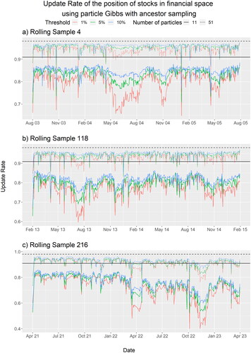
Figure D5. The area under ROC over each rolling sample (date referred to the last trading day in each rolling sample) and each of the network $Y_{1\%}(t)$ (red), $Y_{5\%}(t)$ (green), and $Y_{10\%(t)}$ (blue) respectively using $Q+1=11$ (solid) and $Q+1=51$ (dashed) particles.

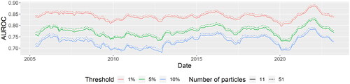
Table D1. The average finalized step size of each parameter and of each systemic risk score when using $Q+1=11$ and $Q+1=51$ particles.

	$Q+1=11$ particles			$Q+1=51$ particles
Parameter	$S_{1\%}(t)$	$S_{5\%}(t)$	$S_{10\%}(t)$	$S_{1\%}(t)$	$S_{5\%}(t)$	$S_{10\%}(t)$
$\mu$	1.738723	0.973832	0.717214	1.043011	0.606951	0.467164
$\Gamma$	0.103985	0.056524	0.042808	0.099816	0.054211	0.041995
$\tau$	0.181385	0.258360	0.328785	0.245882	0.316626	0.374377
${\beta }_1$	0.099375	0.106061	0.121271	0.097452	0.111889	0.122300
${\beta }_2$	0.271351	0.251628	0.261018	0.285235	0.252159	0.262383
${\beta }_3$	0.150813	0.189149	0.228138	0.153746	0.188784	0.234751
${\beta }_4$	0.042307	0.036819	0.038410	0.046244	0.041545	0.041242

Table D2. The minimum, mean, and maximum of the average acceptance rates over all parameters during each MCMC stage and of each systemic risk score when using $Q+1=11$ particles.

MCMC Stage	Threshold	Minimum	Mean	Maximum
During Burn-in	$1\%$	0.303654	0.322675	0.351120
During Burn-in	$5\%$	0.294780	0.313179	0.340088
During Burn-in	$10\%$	0.293593	0.308662	0.338318
After Burn-in	$1\%$	0.248657	0.275436	0.346686
After Burn-in	$5\%$	0.240788	0.271496	0.338175
After Burn-in	$10\%$	0.248701	0.272754	0.340517
Whole Period	$1\%$	0.278910	0.299055	0.346471
Whole Period	$5\%$	0.271535	0.292337	0.339131
Whole Period	$10\%$	0.274617	0.290708	0.337472

Table D3. The minimum, mean, and maximum of the average acceptance rates over all parameters during each MCMC stage and of each systemic risk score when using $Q+1=51$ particles.

MCMC Stage	Threshold	Minimum	Mean	Maximum
During Burn-in	$1\%$	0.303869	0.319336	0.343741
During Burn-in	$5\%$	0.297319	0.313866	0.336855
During Burn-in	$10\%$	0.292256	0.309019	0.335913
After Burn-in	$1\%$	0.247215	0.267012	0.320660
After Burn-in	$5\%$	0.244006	0.271537	0.336203
After Burn-in	$10\%$	0.244733	0.270052	0.334274
Whole Period	$1\%$	0.279660	0.293174	0.327514
Whole Period	$5\%$	0.276296	0.292702	0.333365
Whole Period	$10\%$	0.272125	0.289535	0.333832

Table D4. The minimum, mean, and maximum of the average effective sample size over parameters during each MCMC stage and of each systemic risk score when using $Q+1=11$ particles.

MCMC Stage	Systemic risk score	Minimum	Mean	Maximum
During Burn-in	$S_{1\%}(t)$	247.2302	971.6050	2789.5990
During Burn-in	$S_{5\%}(t)$	237.1198	1579.7918	3286.6614
During Burn-in	$S_{10\%}(t)$	313.1527	1929.2238	3709.4591
After Burn-in	$S_{1\%}(t)$	172.9154	1198.3029	2935.1692
After Burn-in	$S_{5\%}(t)$	108.4546	1790.2548	3516.7451
After Burn-in	$S_{10\%}(t)$	173.8261	2000.7751	3740.1277
Whole Period	$S_{1\%}(t)$	269.9579	1843.9907	5411.6809
Whole Period	$S_{5\%}(t)$	176.0147	2965.6932	6527.4335
Whole Period	$S_{10\%}(t)$	307.4746	3452.3209	7360.1861

Table D5. The minimum, mean, and maximum of the average effective sample size over parameters during each MCMC stage and of each systemic risk score when using $Q+1=51$ particles.

MCMC Stage	Systemic Risk Score	Minimum	Mean	Maximum
During Burn-in	$S_{1\%}(t)$	260.8885	906.0883	2794.9989
During Burn-in	$S_{5\%}(t)$	346.5085	1368.8373	3655.0702
During Burn-in	$S_{10\%}(t)$	309.2980	1681.0046	3706.8096
After Burn-in	$S_{1\%}(t)$	319.2177	1223.7655	3159.9979
After Burn-in	$S_{5\%}(t)$	250.5999	1586.4424	3945.1603
After Burn-in	$S_{10\%}(t)$	225.7158	1730.3827	3917.7699
Whole Period	$S_{1\%}(t)$	483.3355	1773.5549	5136.2152
Whole Period	$S_{5\%}(t)$	502.6808	2496.6749	7130.3548
Whole Period	$S_{10\%}(t)$	395.4822	2881.4296	7357.4621

Table D6. The number of stocks, the number of trading days, and the computation time taken for the MCMC of three selected rolling samples.

			$Q+1=11$ particles	$Q+1=51$ particles
Systemic Risk Score	n	T	Time (Hours)	Time (Hours)
$S_{1\%}(t)$	28	495	2.2968724	10.38519
$S_{5\%}(t)$	28	495	2.8051720	11.41509
$S_{10\%}(t)$	28	495	3.8068931	11.09349
$S_{1\%}(t)$	47	490	4.3280688	23.22842
$S_{5\%}(t)$	47	490	4.6679008	24.18710
$S_{10\%}(t)$	47	490	4.5546711	24.63476
$S_{1\%}(t)$	65	493	6.8102844	32.81657
$S_{5\%}(t)$	65	493	6.9016073	34.44303
$S_{10\%}(t)$	65	493	6.3307427	34.49900

Rolling sample 4: $n=28,$ $T=495;$ Rolling sample 118: $n=47,$ $T=490;$ Rolling sample 216: $n=65,$ $T=493$) with using $Q+1=11$ and $Q+1=51$ particles.

Appendix E.

The Multi-Modal Nature of the Posterior Density

To handle the identifiability issue, we have transformed the MCMC iterate as described in Section 3.2. To have the unique representation of the latent positions, after transforming the MCMC iterate, we observe that the posterior density of some latent positions has multiple modes.

Figure E1 displays both the trace plot and density plot of the estimated posterior density for the positions of CNOOC Limited (0883.HK), BOC Hong Kong (2388.HK), and Esprit Holdings (0330.HK) on April 8, 2005 in the first rolling sample. The network used was constructed using a 1% threshold. Despite the transformation being applied to every MCMC iterate, the density plots of most stock on any trading day in each rolling sample exhibit a multi-modal nature. We specifically selected this combination of stocks and trading day to demonstrate the multi-modal nature. The estimated posterior density for the positions of CNOOC Limited (0883.HK) and Esprit Holdings (0330.HK) exhibits multiple modes, while the estimated posterior density for the position of BOC Hong Kong (2388.HK) has a single mode.

Upon examining the trace plot for the selected stock, we observed that the Markov chain traverses across modes throughout the iterations, indicating good mixing of the MCMC iterates for positions of stocks in the financial space.

Supported by Figure E1, even after applying the transformation in Section 3.2 to achieve the unique representation of the latent positions based on the MCMC iterates, the posterior density remains multi-modal and exhibits reflection symmetry across the two axes and the two diagonals. Therefore, as shown in sub-figures (c) and (i) of Figure E1, the posterior mean of a stock in the financial space may lie in a low probability region. It is worth mentioning that even though sub-figure (f) of Figure E1 suggests the possibility of the posterior mean lying in a high probability region, we assert that the posterior density evaluated at the posterior mean is smaller than the posterior density evaluated at the posterior mode. Figure E2 presents the log posterior density of the first rolling sample based on the network constructed using three threshold levels, along with the log posterior density of the posterior mean. We found that the posterior mean has a substantially lower posterior density than any iterate, including the initial values, supporting our choice to prefer the posterior mode to the posterior mean when computing the systemic risk score and determining reused values used in partial estimation.

Figure E1. The MCMC trace plot (a, b, d, e, g, h) and the density plot (c, f, i) of CNOOC Limited (0883.HK) (a-c), BOC Hong Kong (2388.HK) (d-f), and Esprit Holdings (0330.HK) (g-i) on 8 April 2005 in the first rolling sample. The red cross indicates the estimated posterior mean.

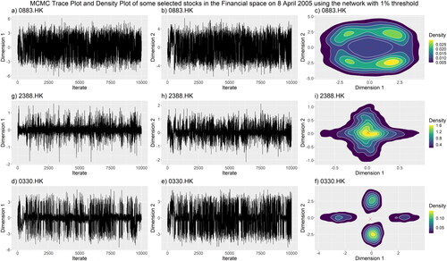
Figure E2. The log posterior density of the first rolling sample based on the network constructed by the three threshold levels (1% Threshold: (a); 5% Threshold: (b); 10% Threshold: (c)). The red horizontal line indicates the log posterior density evaluated at the posterior mean.

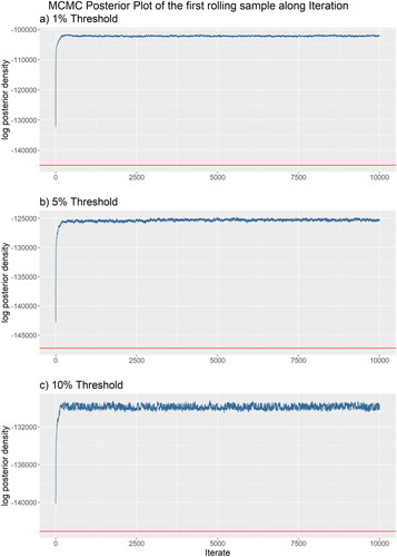
Appendix F.

Details on the Identifiability Issue

F.1 Definition of Unidentified Model

Let $\Theta$ be the parameters space and $\theta \in \Theta$ be the model parameter, such that we have (F1) $$\theta =\left\{\right\{z_{i,t}\},\{{\mu }_i\},\{{\Gamma }_i\},\{{\tau }_i\},\beta \}$$(F1) in our study.

Let ${\Theta }_0\subset \Theta$ be a subset of the parameter space so that the probability of ${\Theta }_0$ in the prior is zero. Referring to the result in Florens and Simoni (2021), the model is unidentified when for any ${\Theta }_0$ there exist two distinct $\theta ,\widehat{\theta }\in \Theta -{\Theta }_0$ such that for any $\mathcal{Y},$ we have (F2) $$\hspace{0.17em}\mathrm{\text{log}}\hspace{0.17em}p(\theta |\mathcal{Y})=\hspace{0.17em}\mathrm{\text{log}}\hspace{0.17em}p(\widehat{\theta }|\mathcal{Y}).$$(F2)

Recall that according to Equation (15)(15) $$\begin{array}{cc}\hspace{0.17em}\mathrm{\text{log}}\hspace{0.17em}p(\mathcal{Z},\beta ,\mu ,\tau ,\Gamma |\mathcal{Y})\hfill & \hfill \\ =\hspace{0.17em}\mathrm{\text{log}}\hspace{0.17em}\mathcal{L}(\mathcal{Y}|\mathcal{Z},\beta ,\mu ,\tau ,\Gamma )+\hspace{0.17em}\mathrm{\text{log}}\hspace{0.17em}\pi (\mathcal{Z},\beta ,\mu ,\tau ,\Gamma ),\hfill & \hfill \end{array}$$(15) , the log posterior is the sum of the log likelihood, log prior densities, and a constant term, i.e. the marginal likelihood of the observed data. The constant term is excluded because it has no effect when we change the parameters. Therefore, we have, after excluding the constant term (F3) $$\hspace{0.17em}\mathrm{\text{log}}\hspace{0.17em}p(\theta |\mathcal{Y})=\hspace{0.17em}\mathrm{\text{log}}\hspace{0.17em}\mathcal{L}(\mathcal{Y}|\theta )+\hspace{0.17em}\mathrm{\text{log}}\hspace{0.17em}\pi (\theta ).$$(F3)

Therefore, the Equation (F2)(F2) $$\hspace{0.17em}\mathrm{\text{log}}\hspace{0.17em}p(\theta |\mathcal{Y})=\hspace{0.17em}\mathrm{\text{log}}\hspace{0.17em}p(\widehat{\theta }|\mathcal{Y}).$$(F2) becomes (F4) $$\hspace{0.17em}\mathrm{\text{log}}\hspace{0.17em}\mathcal{L}(\theta |\mathcal{Y})+\hspace{0.17em}\mathrm{\text{log}}\hspace{0.17em}\pi (\theta )=\hspace{0.17em}\mathrm{\text{log}}\hspace{0.17em}\mathcal{L}(\widehat{\theta }|\mathcal{Y})+\hspace{0.17em}\mathrm{\text{log}}\hspace{0.17em}\pi (\widehat{\theta }).$$(F4)

In other words, the model is unidentified when multiple possible values give the same posterior density. In the following section, we demonstrate that this happens in our model and how we solve this issue.

F.2 Identification Issue Due to the Log Likelihood

Since the log likelihood depends on the distance between the latent positions, instead of the latent positions themselves, as discussed in Section 3.2, any rigid transformation of the financial space is invariant to the log likelihood.

Suppose we first rotate the financial space around the origin, reflect along the axes, and then translate the financial space. We summarize rotation and reflection by an orthogonal matrix $\mathcal{R}$ and the translation by a vector $\delta ,$ so that for every $\theta ,$ we have (F5) $$\widehat{\theta }=\left\{\right\{\delta +\mathcal{R}{z}_{i,t}\},\{\delta +\mathcal{R}{\mu }_i\},\{\mathcal{R}{\Gamma }_i{\mathcal{R}}^{\top }\},\{\mathcal{R}{\tau }_i{\mathcal{R}}^{\top }\},\beta \}$$(F5) satisfying $\theta \ne \widehat{\theta }$ and (F6) $$\hspace{0.17em}\mathrm{\text{log}}\hspace{0.17em}\mathcal{L}(\theta |\mathcal{Y})=\hspace{0.17em}\mathrm{\text{log}}\hspace{0.17em}\mathcal{L}(\widehat{\theta }|\mathcal{Y}).$$(F6)

Therefore, the log likelihood in Equation (F4)(F4) $$\hspace{0.17em}\mathrm{\text{log}}\hspace{0.17em}\mathcal{L}(\theta |\mathcal{Y})+\hspace{0.17em}\mathrm{\text{log}}\hspace{0.17em}\pi (\theta )=\hspace{0.17em}\mathrm{\text{log}}\hspace{0.17em}\mathcal{L}(\widehat{\theta }|\mathcal{Y})+\hspace{0.17em}\mathrm{\text{log}}\hspace{0.17em}\pi (\widehat{\theta }).$$(F4) cancels out. The identification issue occurs when the $\hspace{0.17em}\mathrm{\text{log}}\hspace{0.17em}$ prior density is equal, i.e. (F7) $$\hspace{0.17em}\mathrm{\text{log}}\hspace{0.17em}\pi (\theta )=\hspace{0.17em}\mathrm{\text{log}}\hspace{0.17em}\pi (\widehat{\theta }).$$(F7)

To avoid identification issues due to the rigid transformation of the financial space, we have to assign a suitable prior and set up constraints to the model parameters to guarantee that among all possible $\delta$ and $\mathcal{R},$ the only $\widehat{\theta }$ satisfying Equation (F7)(F7) $$\hspace{0.17em}\mathrm{\text{log}}\hspace{0.17em}\pi (\theta )=\hspace{0.17em}\mathrm{\text{log}}\hspace{0.17em}\pi (\widehat{\theta }).$$(F7) is $\theta .$

F.3 Addressing the Identification Issue Due to Translation

Denote ${\widehat{z}}_{i,t}:=\delta +\mathcal{R}{z}_{i,t},$ ${\widehat{\mu }}_i:=\delta +\mathcal{R}{\mu }_i,$ ${\widehat{\Gamma }}_i:=\mathcal{R}{\Gamma }_i{\mathcal{R}}^{\top },$ and ${\widehat{\tau }}_i:=\mathcal{R}{\tau }_i{\mathcal{R}}^{\top }$ as the position of stock i on trading day t in the financial space, the average position of stock i in the financial space, the diagonal matrix of the persistence of stock i in the financial space, and the diagonal matrix of transition size of stock i in the financial space respectively indicated by $\widehat{\theta }.$ We also denote $\widehat{\mathcal{Z}},$ $\widehat{\mu },$ $\widehat{\Gamma },$ and $\widehat{\tau }$ as the collection of all ${\widehat{z}}_{i,t},$ ${\widehat{\mu }}_i,$ ${\widehat{\Gamma }}_i,$ and ${\widehat{\tau }}_i$ respectively.

According to Equations (8)(8) $$z_{i,1}\sim N({\mu }_i,{(I-{\Gamma }_i^2)}^{-1}{\tau }_i^2),$$(8) and (9)(9) $$z_{i,t}|z_{i,t-1}\sim N({\mu }_i+{\Gamma }_i(z_{i,t-1}-{\mu }_i),{\tau }_i^2).$$(9) , the normal prior of the latent positions $\mathcal{Z}$ given $\mu ,$ $\Gamma ,$ and $\tau$ evaluated at both $\theta$ and $\widehat{\theta }$ are identical. Therefore, to address the identification issue due to translation, we have set up a suitable prior for $\mu .$

In our study, the log prior density of $\mu ,$ after excluding the constant term and substituting the hyperparameters, is (F8) $$\hspace{0.17em}\mathrm{\text{log}}\hspace{0.17em}p(\mu )=-\frac{1}{20}\sum _i{\mu }_i^{\top }{\mu }_i.$$(F8)

Further substituting Equation (F5)(F5) $$\widehat{\theta }=\left\{\right\{\delta +\mathcal{R}{z}_{i,t}\},\{\delta +\mathcal{R}{\mu }_i\},\{\mathcal{R}{\Gamma }_i{\mathcal{R}}^{\top }\},\{\mathcal{R}{\tau }_i{\mathcal{R}}^{\top }\},\beta \}$$(F5) into Equation (F8)(F8) $$\hspace{0.17em}\mathrm{\text{log}}\hspace{0.17em}p(\mu )=-\frac{1}{20}\sum _i{\mu }_i^{\top }{\mu }_i.$$(F8) , we have (F9) $$\hspace{0.17em}\mathrm{\text{log}}\hspace{0.17em}p(\widehat{\mu })=-\frac{1}{20}\sum _i{\delta }^{\top }\delta +2{\delta }^{\top }\mathcal{R}{\mu }_i+{\mu }_i^{\top }{\mu }_i.$$(F9)

Equation (F8)(F8) $$\hspace{0.17em}\mathrm{\text{log}}\hspace{0.17em}p(\mu )=-\frac{1}{20}\sum _i{\mu }_i^{\top }{\mu }_i.$$(F8) equals the Equation (F9)(F9) $$\hspace{0.17em}\mathrm{\text{log}}\hspace{0.17em}p(\widehat{\mu })=-\frac{1}{20}\sum _i{\delta }^{\top }\delta +2{\delta }^{\top }\mathcal{R}{\mu }_i+{\mu }_i^{\top }{\mu }_i.$$(F9) for every $\theta$ if and only if the translation vector $\delta$ is zero. In other words, the prior of $\mu$ addresses the identification issue due to translation.

F.4 Addressing the Identification Issue Due to Arbitrary Rotation

Equation (F5)(F5) $$\widehat{\theta }=\left\{\right\{\delta +\mathcal{R}{z}_{i,t}\},\{\delta +\mathcal{R}{\mu }_i\},\{\mathcal{R}{\Gamma }_i{\mathcal{R}}^{\top }\},\{\mathcal{R}{\tau }_i{\mathcal{R}}^{\top }\},\beta \}$$(F5) lists all outcomes of rigid transformation in the financial space, based on $\delta$ and $\mathcal{R}.$ On one hand, the transformation given by $\delta$ has been eliminated by the normal prior of $\mu .$ On the other hand, we also notice that not all $\mathcal{R}$ give a legitimate $\widehat{\theta }$ as a parameter to the model since we have assumed both ${\Gamma }_i$ and ${\tau }_i$ are diagonal matrices. Therefore, we require ${\widehat{\Gamma }}_i,$ when serving as a legitimate parameter to the model, to be also a diagonal matrix.

Therefore, in the case of $D=2$ dimensional, the orthogonal matrix $\mathcal{R}$ has to satisfy either

• The diagonal entries are zero, and the off-diagonal entries are either $-1$ or 1; or

• The diagonal entries are either $-1$ or 1, and the off-diagonal entries are zero.

This requirement is satisfied when we either rotate the financial space about the origin by multiples of $\pi /2,$ reflect along the axes, or perform any sequence of these two operations.

To emphasize that the orthogonal matrix is no longer arbitrary, we introduce the permutation matrix $\mathcal{P}$ and the reflection matrix $\iota$ as in Section 3.2. The permutation matrix indicates which entry in each column of $\mathcal{R}$ is non-zero. The reflection matrix governs the sign of the non-zero entry in each column of $\mathcal{R}.$ The Equation (F5)(F5) $$\widehat{\theta }=\left\{\right\{\delta +\mathcal{R}{z}_{i,t}\},\{\delta +\mathcal{R}{\mu }_i\},\{\mathcal{R}{\Gamma }_i{\mathcal{R}}^{\top }\},\{\mathcal{R}{\tau }_i{\mathcal{R}}^{\top }\},\beta \}$$(F5) becomes (F10) $$\widehat{\theta }=\left\{\right\{\mathcal{P}\iota z_{i,t}\},\{\mathcal{P}\iota {\mu }_i\},\{\mathcal{P}{\Gamma }_i{\mathcal{P}}^{\top }\},\{\mathcal{P}{\tau }_i{\mathcal{P}}^{\top }\},\beta \}$$(F10) and now always fit as a parameter to the model.

The two constraints applied to each MCMC iterate, as introduced in Section 3.2, have fixed the permutation matrix $\mathcal{P}$ and the reflection matrix $\iota$ in Equation (F10)(F10) $$\widehat{\theta }=\left\{\right\{\mathcal{P}\iota z_{i,t}\},\{\mathcal{P}\iota {\mu }_i\},\{\mathcal{P}{\Gamma }_i{\mathcal{P}}^{\top }\},\{\mathcal{P}{\tau }_i{\mathcal{P}}^{\top }\},\beta \}$$(F10) . Therefore, there is only one $\widehat{\theta }$ satisfying Equation (F7)(F7) $$\hspace{0.17em}\mathrm{\text{log}}\hspace{0.17em}\pi (\theta )=\hspace{0.17em}\mathrm{\text{log}}\hspace{0.17em}\pi (\widehat{\theta }).$$(F7) , and hence the identification issue due to rigid transformation in the financial space is solved.

References

- Abbassi P, Brownlees C, Hans C, Podlich N. 2017. Credit risk interconnectedness: What does the market really know? J Financ Stab. 29:1–12. https://www.sciencedirect.com/science/article/pii/S1572308917300311.
- Acemoglu D, Ozdaglar A, Tahbaz-Salehi A. 2015. Systemic risk and stability in financial networks. Am Econ Rev. 105(2):564–608.
- Acharya VV, Pedersen LH, Philippon T, Richardson M. 2017. Measuring systemic risk. Rev Financ Stud. 30(1):2–47.
- Adrian T, Brunnermeier MK. 2016. Covar. Am Econo Rev. 106(7):1705–1741.
- Aiyar S. 2012. From financial crisis to great recession: the role of globalized banks. Am Econom Rev. 102(3):225–230.
- Allaj E, Sanfelici S. 2022. Early warning systems for identifying financial instability. International Journal of Forecasting; [accessed] https://www.sciencedirect.com/science/article/pii/S0169207022001133.
- Ando T. 2009. Bayesian portfolio selection using a multifactor model. Int J Forecast. 25(3):550–566. https://www.sciencedirect.com/science/article/pii/S016920700900003X.
- Ballester L, López J, Pavía JM. 2023. European systemic credit risk transmission using Bayesian networks. Res Int Busin Finance. 65:101914. https://www.sciencedirect.com/science/article/pii/S0275531923000405.
- Battista GD, Eades P, Tamassia R, Tollis IG. 1994. Algorithms for drawing graphs: an annotated bibliography. Comput Geom. 4(5):235–282. https://www.sciencedirect.com/science/article/pii/092577219400014X.
- Battiston S, Puliga M, Kaushik R, Tasca P, Caldarelli G. 2012. DebtRank: Too central to fail? Financial networks, the FED and systemic risk. Scient Rep. 2(1):1–6.
- Benoit S, Colliard JE, Hurlin C, Pérignon C. 2017. Where the risks lie: a survey on systemic risk. Rev Finance. 21(1):109–152.
- Bhar R, Nikolova B. 2013. Measuring the interconnectedness of financial institutions. Economic Syst. 37(1):17–29. https://www.sciencedirect.com/science/article/pii/S0939362512000775.
- Billio M, Casarin R, Costola M, Pasqualini A. 2016. An entropy-based early warning indicator for systemic risk. J Int Financ Markets Instit Money. 45:42–59.
- Billio M, Getmansky M, Lo AW, Pelizzon L. 2012. Econometric measures of connectedness and systemic risk in the finance and insurance sectors. J Financ Econom. 104(3):535–559.
- Blei SK, Ergashev B. 2014. Asset commonality and systemic risk among large banks in the United States. Available at SSRN 2503046.
- Brownlees C, Engle RF. 2017. SRISK: a conditional capital shortfall measure of systemic risk. Rev Financ Stud. 30(1):48–79.
- Brunnermeier MK. 2009. Deciphering the liquidity and credit crunch 2007–2008. J Econom Persp. 23(1):77–100.
- Cai J, Eidam F, Saunders A, Steffen S. 2018. Syndication, interconnectedness, and systemic risk. J Financ Stabil. 34:105–120. https://www.sciencedirect.com/science/article/pii/S1572308917303698.
- Chan LSH, Chu AMY, So MKP. 2023. A moving-window Bayesian network model for assessing systemic risk in financial markets. PLoS One. 18(1):e0279888.
- Chan N, Getmansky M, Haas SM, Lo AW. 2005. Systemic risk and hedge funds. National Bureau of Economic Research. Working Paper 11200; [accessed]. http://www.nber.org/papers/w11200.
- Chen L, Han Q, Qiao Z, Stanley HE. 2020. Correlation analysis and systemic risk measurement of regional, financial and global stock indices. Physica A. 542:122653.
- Chopin N, Singh SS. 2015. On particle Gibbs sampling. Bernoulli. 21(3):1855–1883.
- Chu AMY, Chan TWC, So MKP, Wong WK. 2021. Dynamic network analysis of COVID-19 with a latent pandemic space model. Int J Environ Res Public Health. 18(6):3195.
- Chu AMY, Chong ACY, Lai NHT, Tiwari A, So MKP. 2023. Enhancing the predictive power of google trends data through network analysis: infodemiology study of Covid-19. JMIR Public Health Surveill. 9(1):e42446.
- Chu AMY, Tiwari A, So MKP. 2020. Detecting early signals of covid-19 global pandemic from network density. J Travel Med. 27(5):taaa084.
- Contreras S, Delis MD, Ghosh A, Hasan I. 2022. Bank failures, local business dynamics, and government policy. Small Bus Econ. 58(4):1823–1851.
- Das SR. 2016. Matrix metrics: network-based systemic risk scoring. J Alterna Invest. 18(4):33–51.
- De Bandt O, Hartmann P. 2000. Systemic risk: a survey. Available at SSRN 258430.
- De Nicolo G, Kwast ML. 2002. Systemic risk and financial consolidation: Are they related? J Bank Finance. 26(5):861–880.
- Deng G, Matteson DS. 2022. Bayesian spillover graphs for dynamic networks. In: Uncertainty in Artificial Intelligence. PMLR. p. 529–538.
- Diebold FX, Yılmaz K. 2014. On the network topology of variance decompositions: measuring the connectedness of financial firms. J Economet. 182(1):119–134.
- Dwyer GP, Tkac P. 2009. The financial crisis of 2008 in fixed-income markets. J Int Money Finance. 28(8):1293–1316.
- Florens JP, Simoni A. 2021. Revisiting identification concepts in bayesian analysis. Ann Econom Statist. 2021(144):1–38.
- Gandy A, Veraart LA. 2017. A Bayesian methodology for systemic risk assessment in financial networks. Manage Sci. 63(12):4428–4446.
- Gelman A, Gilks WR, Roberts GO. 1997. Weak convergence and optimal scaling of random walk metropolis algorithms. Ann Appl Probab. 7(1):110–120.
- Gerlach M, Peixoto TP, Altmann EG. 2018. A network approach to topic models. Sci Adv. 4(7):eaaq1360.
- Giao BC, Anh DT. 2016. Similarity search for numerous patterns over multiple time series streams under dynamic time warping which supports data normalization. Vietnam J Comput Sci. 3(3):181–196.
- Giorgino T. 2009. Computing and visualizing dynamic time warping alignments in R: the dtw package. J Stat Soft. 31(7):1–24.
- Girardi G, Ergün AT. 2013. Systemic risk measurement: multivariate GARCH estimation of CoVaR. J Bank Finance. 37(8):3169–3180.
- Haldane AG, May RM. 2011. Systemic risk in banking ecosystems. Nature. 469(7330):351–355.
- Han D. Khoojine AS. 2019. Network analysis of the Chinese stock market during the turbulence of 2015–2016 using log-returns, volumes and mutual information. Physica A. 523:1091–1109.
- Hanson SG, Kashyap AK, Stein JC. 2011. A macroprudential approach to financial regulation. J Economic Perspect. 25(1):3–28.
- Härdle WK, Wang W, Yu L. 2016. Tenet: tail-event driven network risk. J Economet. 192(2):499–513.
- Hautsch N, Schaumburg J, Schienle M. 2015. Financial network systemic risk contributions. Rev Finance. 19(2):685–738.
- He Z, Krishnamurthy A. 2019. A macroeconomic framework for quantifying systemic risk. Am Economic J. 11(4):1–37.
- Heimo T, Saramäki J, Onnela JP, Kaski K. 2007. Spectral and network methods in the analysis of correlation matrices of stock returns. Physica A. 383(1):147–151.
- Hoff PD, Raftery AE, Handcock MS. 2002. Latent space approaches to social network analysis. J Am Stat Assoc. 97(460):1090–1098.
- Huang X, Vodenska I, Havlin S, Stanley HE. 2013. Cascading failures in bi-partite graphs: model for systemic risk propagation. Sci Rep. 3(1):1–9.
- Hurley JR, Cattell RB. 1962. The procrustes program: producing direct rotation to test a hypothesized factor structure. Behav. Sci. 7(2):258–262.
- Jackson MO, Pernoud A. 2021. Systemic risk in financial networks: a survey. Annu Rev Econ. 13(1):171–202.
- Jiaxing Li ZS. 2022. Stock markets crash in Hong Kong, Shanghai and Shenzhen on a raft of bad news after China’s leadership reshuffle. South China Morning Post; [accessed 2023 Oct 25]. https://www.scmp.com/business/china-business/article/3197041/chinas-leadership-reshuffle-stuns-investors-markets-see-risks-policy-mistakes-shocks-economy.
- Kawata S, Fujiwara Y. 2016. Constructing of network from topics and their temporal change in the Nikkei newspaper articles. Evolut Inst Econ Rev. 13(2):423–436.
- Kritzman M, Li Y, Page S, Rigobon R. 2011. Principal components as a measure of systemic risk. JPM. 37(4):112–126.
- Lai Y, Hu Y. 2021. A study of systemic risk of global stock markets under COVID-19 based on complex financial networks. Physica A. 566:125613.
- Linardi F, Diks C, van der Leij M, Lazier I. 2020. Dynamic interbank network analysis using latent space models. J Economic Dynam Control. 112:103792.
- Lindsten F, Jordan MI, Schon TB. 2014. Particle Gibbs with ancestor sampling. J Mach Learn Res. 15:2145–2184.
- Liu Y. 2018. Hong Kong stocks down a wretched 14 per cent in 2018 – the worst performance in 7 years. South China Morning Post; [accessed 2023 Oct 25]. https://www.scmp.com/business/markets/article/2180077/hong-kong-stocks-get-boost-trump-xi-weekend-phone-call-signalling.
- Lockett H. 2022. China shares fall sharply on concerns over Covid outbreak and Ukraine war. Financial Times; [accessed 2022 Jul 10]. https://www.ft.com/content/528f580a-6770-4940-b8f8-670cf409580a.
- Lupu R, Călin AC, Zeldea CG, Lupu I. 2020. A Bayesian entropy approach to sectoral systemic risk modeling. Entropy. 22(12):1371.
- Maiya AS, Rolfe RM. 2014. Topic similarity networks: visual analytics for large document sets. In: 2014 IEEE International Conference on Big Data (Big Data). p. 364–372.
- Mantegna RN, Stanley HE. 1999. Introduction to econophysics: correlations and complexity in finance. Cambridge: Cambridge University Press.
- Martínez-Jaramillo S, Pérez OP, Embriz FA, Dey FLG. 2010. Systemic risk, financial contagion and financial fragility. J Econom Dynam Control. 34(11):2358–2374.
- Neveu AR. 2018. A survey of network-based analysis and systemic risk measurement. J Econ Interact Coord. 13(2):241–281.
- Ng KC, So MKP, Tam KY. 2021. A latent space modeling approach to interfirm relationship analysis. ACM Trans Manage Inf Syst. 12(2):1–44.
- Patro DK, Qi M, Sun X. 2013. A simple indicator of systemic risk. J Financ Stabil. 9(1):105–116.
- Plummer M, Best N, Cowles K, Vines K. 2006. Coda: convergence diagnosis and output analysis for mcmc. R News. 6(1):7–11.
- Rachev ST, Hsu JS, Bagasheva BS, Fabozzi FJ. 2008. Bayesian methods in finance. Hoboken: John Wiley & Sons.
- Raddant M, Kenett DY. 2021. Interconnectedness in the global financial market. J Int Money Finance. 110:102280.
- Rankin J, Milman O, Ni V. 2021. Global energy crisis: how key countries are responding. The Guardian; [accessed 2022 July 28]. https://www.theguardian.com/business/2021/oct/12/global-energy-crisis-how-key-countries-are-responding.
- Rodríguez-Moreno M, Peña JI. 2013. Systemic risk measures: The simpler the better? J Bank Finance. 37(6):1817–1831.
- Sakoe H, Chiba S. 1978. Dynamic programming algorithm optimization for spoken word recognition. IEEE Trans Acoust, Speech, Signal Process. 26(1):43–49.
- Sewell DK, Chen Y. 2015. Latent space models for dynamic networks. J Am Stat Assoc. 110(512):1646–1657.
- Shin B. 2021. Exploring network measures of social capital: toward more relational measurement. J Plann Literature. 36(3):328–344.
- So MKP, Chan LSH, Chu AMY. 2021a. Financial network connectedness and systemic risk during the COVID-19 pandemic. Asia-Pac Financ Markets. 28(4):649–665.
- So MKP, Chan TWC, Chu AMY. 2020a. Efficient estimation of high-dimensional dynamic covariance by risk factor mapping: applications for financial risk management. J Economet. 227:151–167.
- So MKP, Chu AMY, Chan TWC. 2021b. Impacts of the COVID-19 pandemic on financial market connectedness. Finance Res Lett. 38:101864.
- So MKP, Chu AMY, Lo CCY, Ip CY. 2021c. Volatility and dynamic dependence modeling: review, applications, and financial risk management. Wiley Interdiscip Rev Comput Stat. 2021:e1567.
- So MKP, Mak ASW, Chu AMY. 2022. Assessing systemic risk in financial markets using dynamic topic networks. Sci Rep. 12(1):2668.
- So MKP, Tiwari A, Chu AMY, Tsang JTY, Chan JNL. 2020b. Visualizing Covid-19 pandemic risk through network connectedness. Int J Infect Dis. 96:558–561.
- Tabak BM, Takami M, Rocha JM, Cajueiro DO, Souza SR. 2014. Directed clustering coefficient as a measure of systemic risk in complex banking networks. Physica A. 394:211–216.
- Thurner S, Poledna S. 2013. Debtrank-transparency: controlling systemic risk in financial networks. Sci Rep. 3(1):1888.
- Tomczak K. 2023. Transmission of the 2007–2008 financial crisis in advanced countries of the european union. Bulletin of Econ Res. 75(1):40–64.
- Tormene P, Giorgino T, Quaglini S, Stefanelli M. 2009. Matching incomplete time series with dynamic time warping: an algorithm and an application to post-stroke rehabilitation. Artif Intell Med. 45(1):11–34.
- Ureche-Rangau L, Burietz A. 2013. One crisis, two crises… the subprime crisis and the European sovereign debt problems. Econom Modell. 35:35–44.
- Wang GJ, Xie C, He K, Stanley HE. 2017. Extreme risk spillover network: application to financial institutions. Quant Finance. 17(9):1417–1433.
- Wang GJ, Yi S, Xie C, Stanley HE. 2021. Multilayer information spillover networks: measuring interconnectedness of financial institutions. Quant Finance. 21(7):1163–1185.
- Zhang X, Xu G, Zhu J. 2022. Joint latent space models for network data with high-dimensional node variables. Biometrika. 109(3):707–720.