Adaptive Sequential Singular Spectrum Analysis: Effective Signal Extraction with Application to Heart Rate Signals Related to E-Cigarette Use

Abstract

The Singular Spectrum Analysis (SSA) is a useful tool for extracting signals from noisy time series. However, the structural insights provided by SSA are significantly influenced by the choice of window length. While the conventional approach, recommending a larger window length, excels with short to moderately-sized time series, it becomes computationally burdensome for longer time series, potentially amplifying mean squared reconstruction errors. This study addresses this methodological gap by introducing an adaptive sequential SSA method that iteratively selects an optimal window length for efficient extraction of essential eigen-sequences (signals) with minimal reconstruction error. This proposed method is versatile, catering to both short-moderate and lengthy time series. Simulation studies demonstrate its efficacy in scenarios where observed data stem from the sum of two sinusoidal functions and noise. Real data analysis on 6-day heart rate data from a young adult e-cigarette user reveals a distinct clustering of vaping events in the scatter plot of the first and third eigen-sequences, indicating the potential of developing “digital biomarkers” for vaping behavior based on extracted eigen-sequences in future studies. In conclusion, the adaptive sequential SSA method offers a robust and flexible approach for signal extraction in diverse time series applications.

Keywords:

• Singular spectrum analysis
• singular value decomposition
• e-cigarette
• heart rate

1. Introduction

The Singular Spectrum Analysis (SSA) is a useful method to find periodical trends to extract signals from noisy time series. Although the SSA method is commonly attributed to Broomhead and King (1986); Broomhead, King, et al. (1986), the original work could be traced back to de Prony (1795) according to Golyandina and Zhigljavsky (2020). Since its inception, the basic SSA algorithm – consisting of four steps – has remained unchanged. In the first step, given a time series and a fixed window length, the embedding procedure maps the time series into a Hankel matrix, the size of which is determined by the window length. The second step involves Singular Value Decomposition (SVD) that decomposes the Hankel matrix into a sum of rank-one matrices. The third step, known as the eigentriple grouping, selects a subset of rank-one matrices which are by convention the top few rank-one matrices based on singular values. The fourth step, hankelization, involves mapping the sum of the matrices selected in Step 3 into a one-dimensional vector through diagonal averaging. As described above, this algorithm requires a priori knowledge of the window length that creates practical issues as we analyzed intensive heart rate data from e-cigarette users who wore smartwatches for 7 days.

Our work with heart rate data found that the structural details revealed by SSA are, in fact, heavily influenced by the choice of window length. The conventional approach recommends adopting close to a half of the time series length as the window length. Yet, this recommendation is impractical for analyzing long time series like heart rate data as a large window length requires specialized methods involving expensive computation to conduct SVD on large Hankel matrices. Additionally, a large window length increases reconstruction errors. Furthermore, the eigentriple grouping is also constrained by the same window length that could potentially lead to missing important details in heart rate patterns that may be otherwise identified using different window lengths.

This study aims to address this methodological issue of SSA by developing an innovative method to estimate the window length adaptively and employ rank-two approximation to identify sequences sequentially. This method can be applied to identify heart rate patterns related to vaping behavior that may be used in future intervention trials. This paper is organized as follows. Section 2 reviews SSA and the effect of window length on SSA. The proposed method is described in detail in Section 3. In Section 4, the proposed method is evaluated by simulation studies and its application is demonstrated by the heart rate data that motivated this study. Section 5 concludes the findings of this study and discusses future research.

2. Existing Methodology and Related Challenges

2.1. Review of Singular Spectrum Analysis (SSA)

SSA is conducted on a centered time series sequence $x_1,x_2,\dots ,x_N$ of length N, with two tuning parameters: the window length w ($\le N/2$); and the number of groups r ($\le w$). The SSA procedure consists of the following four steps.

First, define the column vector ${\mathit{x}}_j={(x_j,x_{j+1},\dots ,x_{j+w-1})}^T,$ where $j=1,\dots ,N-w+1.$ The resulting matrix $X=({\mathit{x}}_1,\dots ,{\mathit{x}}_{N-w+1})$ is thus a Hankel matrix because the elements along each anti-diagonal are equal.

Second, the Singular Value Decomposition (SVD) is applied to express the matrix X as $X={\mathit{\text{USV}}}^T={\sum }_{k=1}^w{\sigma }_k{\mathit{u}}_k{\mathit{v}}_k^T,$ where ${\sigma }_1\ge \dots \ge {\sigma }_w\ge 0$ are the singular values of X. Here, $U=({\mathit{u}}_1,\dots ,{\mathit{u}}_w)$ is the left singular matrix, $V=({\mathit{v}}_1,\dots ,{\mathit{v}}_w)$ is the right singular matrix, and $S=\text{diag}({\sigma }_1,\dots ,{\sigma }_w).$

Third, define $\widehat{X}={\sum }_{k=1}^r{\sigma }_k{\mathit{u}}_k{\mathit{v}}_k^T.$ Thus, $\widehat{X}$ represents the rank-r approximation of X.

Fourth, Hankelization is conducted to map the matrix $\widehat{X}$ to a vector through diagonal averaging. Detailed steps of the SSA algorithm can be found in references such as Golyandina, Korobeynikov, and Zhigljavsky (2018); Golyandina and Zhigljavsky (2020); Sanei and Hassani (2015).

2.2. Existing Methods for Window Length Selection

One crucial parameter in the SSA method is the window length w, which significantly affects the reconstructed time series. The choice of window length is pivotal in achieving accurate reconstruction. Traditionally, the selection of window length in SSA has often relied on empirical experience or guidelines, which may not be universally applicable across time series with various noise to signal ratios or different patterns of signals Cong et al. (2015); Unnikrishnan and Jothiprakash (2019). In practical scenarios, this approach often involves a trial-and-error process through various window lengths to find the most suitable one for a specific data set.

For periodic time series, periodogram analysis is often conducted to estimate the periodic frequency. The window length can then be chosen as an integer multiple of half the oscillation period Sun, Li, et al. (2017); Yang et al. (2016). Simulation studies, however, have shown that this approach does not necessarily lead to improved accuracy Knapik et al. (2022).

Golyandina (2010) conducted a simulation study and recommended using a window length close to the largest value, $\lfloor N/2\rfloor .$ Another approach, based on the median $(1,2,\dots ,N),$ which is close to $N/2,$ has also been suggested Hassani et al. (2011). Yet, these recommendations are primarily applicable to time series with short to moderate lengths. In fact, prior studies have shown that excessively large values of w, such as $\lfloor N/2\rfloor ,$ could lead to detrimental effects on time series reconstruction, resulting in increased mean squared reconstruction errors Atikur Rahman Khan and Poskitt (2013); Khan, Poskitt, et al. (2010).

To deal with potential issues with adopting a long window length, another recommendation for window length selection was derived under regularity conditions—weak stationarity and ergodicity—as: ${(\hspace{0.17em}\mathrm{\text{log}}\hspace{0.17em}N)}^c,$ where c is restricted to be larger than $\hspace{0.17em}\mathrm{\text{log}}\hspace{0.17em}2/\hspace{0.17em}\mathrm{\text{log}}\hspace{0.17em}\hspace{0.17em}\mathrm{\text{log}}\hspace{0.17em}N$ Atikur Rahman Khan and Poskitt (2013); Khan and Poskitt (2011). Based on this recommendation, the window length is much shorter than $N/2.$

An alternative approach for window length selection is based on the observation that the number of time series sources is related to the window length Ma et al. (2012); Wang et al. (2015). The autocorrelation matrix of time series is adopted to determine the number of sources that is then used to choose the window length. There are, however, two issues with this approach. First, it assumes that the sources are additive and each source has only one fixed frequency. Second, it tends to select smaller window lengths, which can result in larger reconstruction errors, according to the simulation study by Golyandina (2010).

In summary, existing methods for window length selection have important limitations. First, they may not adequately account for complex patterns or trends present in the data. Second, they may make assumptions about the underlying structure of time series, such as stationarity, which may not hold in practice. Third, once the window length is determined, the same window length is used to reconstruct series. This may not perform well especially when the underlying sources have different frequencies. In that case, it would be ideal to use a different window length for each frequency to extract signals. Thus, there is a pressing need for a more robust and flexible method to determine the optimal window length(s), one that can accommodate diverse data characteristics and provide accurate reconstructions across a wide range of scenarios.

2.3. The Impact of Window Length on SSA

To evaluate the influence of window length on SSA, we examine a noiseless simple harmonic function given by $\mathit{x}=\hspace{0.17em}\mathrm{\text{cos}}\hspace{0.17em}(2\pi f·1),\hspace{0.17em}\mathrm{\text{cos}}\hspace{0.17em}(2\pi f·2),\dots ,\hspace{0.17em}\mathrm{\text{cos}}\hspace{0.17em}(2\pi f·N),$ where f denotes frequency. For a chosen window length $w(>2),$ the corresponding matrix X is expressed as (1) $$X=\left(\begin{array}{cccc}\hspace{0.17em}\mathrm{\text{cos}}\hspace{0.17em}(2\pi f·1)& \hspace{0.17em}\mathrm{\text{cos}}\hspace{0.17em}(2\pi f·2)& \dots & \hspace{0.17em}\mathrm{\text{cos}}\hspace{0.17em}(2\pi f·c)\\ \hspace{0.17em}\mathrm{\text{cos}}\hspace{0.17em}(2\pi f·2)& \hspace{0.17em}\mathrm{\text{cos}}\hspace{0.17em}(2\pi f·3)& \dots & \hspace{0.17em}\mathrm{\text{cos}}\hspace{0.17em}(2\pi f·(c+1))\\ ⋮& ⋮& \ddots & ⋮\\ \hspace{0.17em}\mathrm{\text{cos}}\hspace{0.17em}(2\pi f·w)& \hspace{0.17em}\mathrm{\text{cos}}\hspace{0.17em}(2\pi f·(w+1))& \dots & \hspace{0.17em}\mathrm{\text{cos}}\hspace{0.17em}(2\pi f·N)\end{array}\right)$$(1) where $c=N-w+1.$ Notably, the rank of X in Equation (1)(1) $$X=\left(\begin{array}{cccc}\hspace{0.17em}\mathrm{\text{cos}}\hspace{0.17em}(2\pi f·1)& \hspace{0.17em}\mathrm{\text{cos}}\hspace{0.17em}(2\pi f·2)& \dots & \hspace{0.17em}\mathrm{\text{cos}}\hspace{0.17em}(2\pi f·c)\\ \hspace{0.17em}\mathrm{\text{cos}}\hspace{0.17em}(2\pi f·2)& \hspace{0.17em}\mathrm{\text{cos}}\hspace{0.17em}(2\pi f·3)& \dots & \hspace{0.17em}\mathrm{\text{cos}}\hspace{0.17em}(2\pi f·(c+1))\\ ⋮& ⋮& \ddots & ⋮\\ \hspace{0.17em}\mathrm{\text{cos}}\hspace{0.17em}(2\pi f·w)& \hspace{0.17em}\mathrm{\text{cos}}\hspace{0.17em}(2\pi f·(w+1))& \dots & \hspace{0.17em}\mathrm{\text{cos}}\hspace{0.17em}(2\pi f·N)\end{array}\right)$$(1) is 2.

Let $B=({\mathit{b}}_c,{\mathit{b}}_s)$ and $C={({\mathit{c}}_c,{\mathit{c}}_s)}^T,$ where $${\mathit{b}}_c={(\hspace{0.17em}\mathrm{\text{cos}}\hspace{0.17em}(2\pi f·1),\hspace{0.17em}\mathrm{\text{cos}}\hspace{0.17em}(2\pi f·2),\dots ,\hspace{0.17em}\mathrm{\text{cos}}\hspace{0.17em}(2\pi f·w))}^T,$$ $${\mathit{b}}_s={(\hspace{0.17em}\mathrm{\text{sin}}\hspace{0.17em}(2\pi f·1),\hspace{0.17em}\mathrm{\text{sin}}\hspace{0.17em}(2\pi f·2),\dots ,\hspace{0.17em}\mathrm{\text{sin}}\hspace{0.17em}(2\pi f·w))}^T,$$ $${\mathit{c}}_c={(\hspace{0.17em}\mathrm{\text{cos}}\hspace{0.17em}(2\pi f·0),\hspace{0.17em}\mathrm{\text{cos}}\hspace{0.17em}(2\pi f·1),\dots ,\hspace{0.17em}\mathrm{\text{cos}}\hspace{0.17em}(2\pi f·(c-1)))}^T,$$ $${\mathit{c}}_s={(-\hspace{0.17em}\mathrm{\text{sin}}\hspace{0.17em}(2\pi f·0),-\hspace{0.17em}\mathrm{\text{sin}}\hspace{0.17em}(2\pi f·1),\dots ,-\hspace{0.17em}\mathrm{\text{sin}}\hspace{0.17em}(2\pi f·(c-1)))}^T.$$

Algebraically, X can be decomposed as (2) $$\begin{array}{c}X=\mathit{\text{BC}}\\ =\left(\begin{array}{cc}\hspace{0.17em}\mathrm{\text{cos}}\hspace{0.17em}(2\pi f·1)& \hspace{0.17em}\mathrm{\text{sin}}\hspace{0.17em}(2\pi f·1)\\ \hspace{0.17em}\mathrm{\text{cos}}\hspace{0.17em}(2\pi f·2)& \hspace{0.17em}\mathrm{\text{sin}}\hspace{0.17em}(2\pi f·2)\\ ⋮& ⋮\\ \hspace{0.17em}\mathrm{\text{cos}}\hspace{0.17em}(2\pi f·w)& \hspace{0.17em}\mathrm{\text{sin}}\hspace{0.17em}(2\pi f·w)\end{array}\right)\left(\begin{array}{cccc}\hspace{0.17em}\mathrm{\text{cos}}\hspace{0.17em}(2\pi f·0)& \hspace{0.17em}\mathrm{\text{cos}}\hspace{0.17em}(2\pi f·1)& \dots & \hspace{0.17em}\mathrm{\text{cos}}\hspace{0.17em}(2\pi f·(c-1))\\ -\hspace{0.17em}\mathrm{\text{sin}}\hspace{0.17em}(2\pi f·0)& -\hspace{0.17em}\mathrm{\text{sin}}\hspace{0.17em}(2\pi f·1)& \dots & -\hspace{0.17em}\mathrm{\text{sin}}\hspace{0.17em}(2\pi f·(c-1))\end{array}\right)\end{array}$$(2)

Note that the vectors ${\mathit{b}}_c$ and ${\mathit{b}}_s$ are independent. Thus, each column vector in X can be represented as a linear combination of ${\mathit{b}}_c$ and ${\mathit{b}}_s.$ Specifically, $${\mathit{x}}_j=\hspace{0.17em}\mathrm{\text{cos}}\hspace{0.17em}(2\pi f·(j-1)){\mathit{b}}_c+(-\hspace{0.17em}\mathrm{\text{sin}}\hspace{0.17em}(2\pi f·(j-1))){\mathit{b}}_s.$$

Hence, the column space of X is spanned by the vectors ${\mathit{b}}_c$ and ${\mathit{b}}_s.$ To achieve a proper decomposition of ${\mathit{x}}_j$ into the vectors ${\mathit{b}}_c$ and ${\mathit{b}}_s,$ the window length w is recommended to be proportional to $1/(2f).$ In practice, when the frequency f is unknown, a larger value for w is often suggested.

The relationship between the window length and the singular values of X may shed some light on finding the optimal window length. Let σ₁ and σ₂ be the positive singular values of X with the rank of 2. The Frobenius norm $\left|\right|X|{|}_F^2={\sigma }_1^2+{\sigma }_2^2,$ which is also equal to the trace of XX^T. Given that $$\begin{array}{c}X{X}^T={\mathit{\text{BCC}}}^T{B}^T\\ =B\left(\begin{array}{cc}{\mathit{c}}_c^T{\mathit{c}}_c& {\mathit{c}}_c^T{\mathit{c}}_s\\ {\mathit{c}}_s^T{\mathit{c}}_c& {\mathit{c}}_s^T{\mathit{c}}_s\end{array}\right)B^T\\ =B\left(\begin{array}{cc}\sum _{j=1}^c(\hspace{0.17em}\mathrm{\text{cos}}\hspace{0.17em}(2\pi f(j-1)){)}^2& -\sum _{j=1}^c\hspace{0.17em}\mathrm{\text{cos}}\hspace{0.17em}(2\pi f(j-1))\hspace{0.17em}\mathrm{\text{sin}}\hspace{0.17em}(2\pi f(j-1))\\ -\sum _{j=1}^c\hspace{0.17em}\mathrm{\text{cos}}\hspace{0.17em}(2\pi f(j-1))\hspace{0.17em}\mathrm{\text{sin}}\hspace{0.17em}(2\pi f(j-1))& \sum _{j=1}^c(\hspace{0.17em}\mathrm{\text{sin}}\hspace{0.17em}(2\pi f(j-1)){)}^2\end{array}\right)B^T\\ =B\left(\begin{array}{cc}\sum _{j=1}^c(\hspace{0.17em}\mathrm{\text{cos}}\hspace{0.17em}(2\pi f(j-1)){)}^2& -0.5\sum _{j=1}^c\hspace{0.17em}\mathrm{\text{sin}}\hspace{0.17em}(4\pi f(j-1))\\ -0.5\sum _{j=1}^c\hspace{0.17em}\mathrm{\text{sin}}\hspace{0.17em}(4\pi f(j-1))& \sum _{j=1}^c(\hspace{0.17em}\mathrm{\text{sin}}\hspace{0.17em}(2\pi f(j-1)){)}^2\end{array}\right)B^T,\end{array}$$

The trace of XX^T can be derived as $$\mathit{\text{tr}}(X{X}^T)=\left(\sum _{j=1}^c(\hspace{0.17em}\mathrm{\text{cos}}\hspace{0.17em}(2\pi f(j-1)){)}^2\right)\left(\sum _{j=1}^w(\hspace{0.17em}\mathrm{\text{cos}}\hspace{0.17em}(2\pi \mathit{\text{fj}}))\right)$$ $$-\left(\sum _{j=1}^c\hspace{0.17em}\mathrm{\text{sin}}\hspace{0.17em}(4\pi f(j-1))\right)\left(\sum _{j=1}^w(\hspace{0.17em}\mathrm{\text{cos}}\hspace{0.17em}(2\pi \mathit{\text{fj}}))(\hspace{0.17em}\mathrm{\text{sin}}\hspace{0.17em}(2\pi \mathit{\text{fj}}))\right)$$ (3) $$+\left(\sum _{j=1}^c(\hspace{0.17em}\mathrm{\text{sin}}\hspace{0.17em}(2\pi f(j-1)){)}^2\right)\left(\sum _{j=1}^w(\hspace{0.17em}\mathrm{\text{sin}}\hspace{0.17em}(2\pi \mathit{\text{fj}}))\right)$$(3)

Thus, for a given simple harmonic time series with one fixed frequency (i.e. f), there are two singular values (σ₁ and σ₂). This result is consistent with prior work by Guo et al. (2020); Zhao and Ye (2019). Specifically, given X, the $\left|\right|X|{|}_F^2$ equals ${\sigma }_1^2+{\sigma }_2^2$ which is equivalent to the value in Equation (3)(3) $$+\left(\sum _{j=1}^c(\hspace{0.17em}\mathrm{\text{sin}}\hspace{0.17em}(2\pi f(j-1)){)}^2\right)\left(\sum _{j=1}^w(\hspace{0.17em}\mathrm{\text{sin}}\hspace{0.17em}(2\pi \mathit{\text{fj}}))\right)$$(3) . This equation demonstrates that the values of σ₁ and σ₂ depend on the window length w. If an improper window length is chosen, we may observed a large value of σ₁ and a very small value of σ₂, resulting in improper low-rank matrix identification. To deal with this methodological issue, this study proposes to choose the window length that produces a pair of singular values closest to each other. This approach tends to produce better rank two approximation.

2.4. Determining the Number of Eigen-Sequences

In conventional SSA, two common approaches are employed to ascertain the number of sequences extracted from the original time series. Since SSA relies on SVD, this inquiry is essentially a question of determining the rank of approximation.

The first approach determines the rank by comparing the sum of squared singular values with a predefined threshold. A widely adopted criterion is to select r such that ${\sum }_{k=1}^r{\sigma }_k^2/{\sum }_{k=1}^w{\sigma }_k^2>0.95.$ The second approach involves evaluating separability between the extracted sequence and the residual sequence using the weighted correlation Golyandina et al. (2001). This approach ensures that the sequences derived from the chosen eigen-triples have high weighted correlation.

These conventional approaches are, however, anchored in a fixed window length. Although the residual series under this fixed window length may not manifest evidence of a signal, such absence of evidence may not be applied to a different window length. To deal with this methodological issue, this study proposes an adaptive sequential approach.

3. The Proposed Adaptive Sequential SSA

In this study, we propose an innovative adaptive sequential SSA method to address the limitations of conventional approaches by dynamically estimating the window length and sequentially identifying signals. These two primary steps are detailed and followed by an algorithm to implement the methodology in the following subsections.

3.1. Dynamic Estimation of Window Length

The objective in selecting the window length w is to ensure the initial pairs of singular values are closely positioned. Given a vector x and a window length w, the first two singular values σ₁ and σ₂ of the derived Hankel matrix X are influenced by the window length. As explained in Section 2.3, the difference ${\sigma }_1-{\sigma }_2$ is a function of window length w and displays local minima at various window lengths. For instance, if the sequence x represents a sinusoidal wave with the frequency f, the difference ${\sigma }_1-{\sigma }_2$ reaches a local minimum when the window length is a multiple of $1/(2f).$ Since the exact frequency f is unknown, we propose to estimate the window length by taking the minimum of all window lengths that produce local minima of ${\sigma }_1-{\sigma }_2.$ This estimated window length is then used to extract the signal and reconstruct the sequence. Because this reconstructed sequence is based on the first two singular values, it represents the optimal rank-two approximation.

3.2. Sequential Eigen-Sequence Identification and Residual Sequence Evaluation

In contrast to conventional SSA, our innovative method extracts sequences sequentially, utilizing a rank-two approximation in each step. Eigen-sequence extraction is concluded when the information remaining in the sequence becomes substantially smaller than that in the original sequence, as indicated by the ratio of standard deviations of the two sequences.

Let s₀ represent the standard deviation of the original time series sequence. Employing the window length determination method outlined in the preceding section, we construct the SVD of the Hankel matrix. In this context, a signal sequence is formed based on a rank-two approximation, termed the eigen-sequence. The residual sequence is derived by computing the difference between the original time series and the eigen-sequence. Let s₁ denote the standard deviation of the residual sequence. If the ratio $s_1/s_0$ falls below a threshold C, it signifies that the variation in the residual sequence is minimal compared to the original time sequence, prompting the algorithm to terminate. Based on our experience with heart rate data, we recommend setting C = 0.1.

3.3. Overall Algorithm

Let the initial sequence be denoted as $\mathit{x}=(x_1,x_2,\dots ,x_N)$ with a standard deviation of s₀. The comprehensive algorithm for our proposed adaptive sequential SSA method is outlined below:

Step 1: Dynamic Window Length Estimation.

Given the input sequence x, window lengths ranging from 2 to half of the sequence length are considered. For each window length, convert the sequence x into the Hankel matrix X. Perform SVD on X and obtain its first two singular values. Identify all window lengths that result in local minima of the difference between the first two singular values. Take the minimum of these window lengths as the estimated window length w.

Step 2: Eigen-sequence Identification.

Execute conventional SSA with a rank-two approximation, ${\sigma }_1{\mathit{u}}_1{\mathit{v}}_1^T+{\sigma }_2{\mathit{u}}_2{\mathit{v}}_2^T,$ based on the estimated window length w from Step 1. Apply hankelization to the rank-two matrix to obtain the eigen-sequence $\tilde{\mathit{x}}.$

Step 3: Residual Sequence Evaluation.

Define the residual sequence as ${\mathit{x}}_{\text{res}}=\mathit{x}-\tilde{\mathit{x}},$ where subtraction is performed element-wise. Let the standard deviation of ${\mathit{x}}_{\text{res}}$ be $s_{\text{res}}.$ If $s_{\text{res}}/s_0<0.1,$ proceed to Step 4. Otherwise, return to Step 1 using ${\mathit{x}}_{\text{res}}$ as the input.

Step 4: Final Reported Eigen-Sequence.

The final reported sequence is the sum of all eigen-sequences $\tilde{\mathit{x}}$ obtained in Step 2.

This adaptive sequential approach ensures that the window length is tailored to the specific characteristics of the time series, and eigen-sequences are identified in a manner that reflects their significance in contributing to the overall structure.

3.4. Time Complexity Analysis

For the conventional method, the computational complexity is $O\left(N{w}^2\right)$ primarily due to the dominance of the SVD step in computation time. In contrast, our proposed method utilizes Reduced SVD (RSVD), specifically a rank 2 SVD, leveraging efficient algorithms such as the Lanczos algorithm Larsen (1998) or the Arnoldi method Lehoucq et al. (1998) implemented in the ARPACK. The computational complexity for each RSVD step is $O\left(2N\mathit{\text{w}}\right)=O\left(N\mathit{\text{w}}\right).$ Considering that the proposed algorithm requires approximately w iterations, the overall complexity remains $O\left(N{w}^2\right),$ which is equivalent to the conventional method.

4. Simulation Studies and Real Data Analysis

To evaluate the effectiveness of our proposed method, we conducted simulation studies under three artificial scenarios based on sinusoidal function(s): (I) a pure sinusoidal function; (II) a sinusoidal function with noise; and III) the sum of two sinusoidal functions and noise. We also applied the proposed method to the heart rate data that motivated this methodology work to demonstrate its applications. Using the reconstructed series from this real data analysis, we conducted Simulation Study IV to compare the proposed method with the conventional SSA in terms of reconstruction errors.

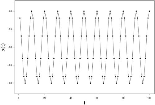
4.1. Simulation Study I: A Pure Sinusoidal Function

In the first simulation study, we examined the relationship between the window length employed in SSA and the selected singular values generated by a pure sinusoidal function with a single frequency. This function is defined as $$x(t)=\hspace{0.17em}\mathrm{\text{cos}}\hspace{0.17em}(2\pi \mathit{\text{ft}}),$$ where $f=0.1$ and $t=1,\dots ,N.$ The temporal pattern of $x(t)$ is visually depicted in Figure 1.

Figure 1. Data of Simulation Study I: the pure sinusoidal function.

Applying the conventional SSA approach, we transformed $x(t)$ into a Hankel matrix $X$ for varying window lengths ranging from 3 to 50. Utilizing SVD, we calculated the first two singular values of $X.$ The results are illustrated in the top panel of Figure 2. Some notable observations emerge from this analysis. First, as the window length increases, the two positive singular values of the matrix $X$ exhibit a generally increasing trend. Second, the difference between the first two singular values displays a periodic change pattern with a decreasing trend alternating with an increasing trend across window lengths. Third, although the values of the first two singular values eventually reaches an asymptote, the difference between them does not converge to zero.

Figure 2. Results of Simulation Study I: the first two singular values of the Hankel matrix (top) and the difference between the top two singular values (bottom) across different window lengths.

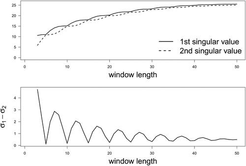
To delve deeper into the relationship between the window length and the difference between the first two singular values, we plotted them in the bottom panel of Figure 2. From this figure, it is evident that the difference between the first two singular values reaches local minima when the window lengths are $5,10,15,20,25,30,35,$ all of which are multiples of 5. This observation confirms that the optimal window length is a multiple of $1/(2f)$ for a pure sinusoidal sequence.

4.2. Simulation Study II: A Sinusoidal Function with Noise

In the second simulation study, we investigated the impact of noise on singular values by adding noise to the function studied in Simulation I, defined as $$y(t)=\hspace{0.17em}\mathrm{\text{cos}}\hspace{0.17em}(2\pi \mathit{\text{ft}})+e(t),$$ where $f=0.1,$ $t=1,\dots ,N,$ and $e(t)$ is normally distributed with a mean of 0 and a standard deviation of 1.5. The temporal pattern of $y(t)$ is presented in Figure 3. Utilizing conventional SSA, the first three singular values of the Hankel matrix for window lengths ranging from 3 to 50 are displayed in the top panel of Figure 4.

Figure 3. Data of Simulation Study II: the sinusoidal function data with noise.

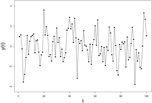
Figure 4. Results of Simulation Study II: The first three singular values of the Hankel matrix (top) and the difference between the top two singular values (bottom) across different window lengths.

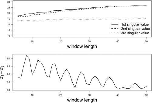
Comparing the top panels of Figures 2 and 4, key observations emerge. In Simulation I, the third singular value is consistently zero for any window length values. However, with a relatively large amount of noise embedded in the observed data in Simulation II, a substantial third singular value is observed for all window length values. This implies that if the selection of $r$ is based on singular values, there is a risk of selecting noise components in conventional SSA.

The difference between the first two singular values is shown in the bottom panel of Figure 4. In Simulation I, local minima of the difference between the first two singular values occur at the window lengths that are multiples of 5. In Simulation II, the window lengths corresponding to local minima of the difference between the first two singular values are 6, 10, 16, 20, 25, 30, 35, 40, 44, and 48. The proposed window length estimation method thus estimates the window length to be 6, which is very close to the theoretical value when there is no noise. Conversely, the conventional SSA approach would recommend using the largest window length (i.e. 50).

Simulations I and II highlight that the first two singular values are dependent on the window length. Using the largest window length does not necessarily select a pair of singular values that are close to each other. It could also possibly lead to the selection of singular values related to noise. Intriguingly, our approach not only indicates that the first two singular values are sufficient but also estimates a window length smaller than the conventionally recommended window length, thereby enhancing the efficiency of the subsequent SVD computation.

4.3. Simulation Study III: The Sum of Two Sinusoidal Functions and Noise

The third simulation study investigated the decomposition of a time series that is the sum of two sinusoidal functions and noise: $$z(t)=3\hspace{0.17em}\mathrm{\text{cos}}\hspace{0.17em}(2\pi f_{1}t)+\hspace{0.17em}\mathrm{\text{sin}}\hspace{0.17em}(2\pi f_{2}t)+{ϵ}_t,$$ where $f_1=0.04,$ $f_2=0.2,$ $t=1,\dots ,100,$ and ${ϵ}_t$ is a random noise following a normal distribution with mean 0 and variance 1. The temporal pattern of $z(t)$ is illustrated in Figure 5. Because $z(t)$ represents the sum of two sinusoidal functions, it inherently possesses four dominant singular values.

Figure 5. Data of Simulation Study III: the sum of two sinusoidal functions and noise.

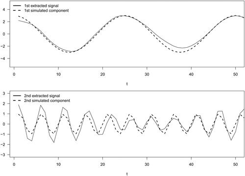
The proposed method was adopted to iteratively construct eigen-sequences. Initially, the estimated window length was 12. The extracted eigen-sequence is visualized in the top panel of Figure 6, with the first component of the function, $3\hspace{0.17em}\mathrm{\text{cos}}\hspace{0.17em}(2\pi f_{1}t),$ being superimposed for the purpose of comparison. The close alignment between these two functions is evident in this figure. Subsequently, the residual sequence that was derived by subtracting this extracted eigen-sequence from $z(t)$ was used to estimate a new window length as 8. The eigen-sequence extracted at this particular length is presented in the bottom panel of Figure 6 with the second simulated component, ($\hspace{0.17em}\mathrm{\text{sin}}\hspace{0.17em}(2\pi f_{2}t)$), being overlaid for the purpose of comparison. Although the second eigen-sequence exhibits a larger amplitude compared to the second simulated component, the frequencies of the two curves match quite well.

Figure 6. Results of Simulation Study III. Top panel: The first eigen-sequence from the proposed method (solid line) and the first component of the simulated function (dashed line). Bottom panel: The second eigen-sequence from the proposed method (solid line) and the second component of the simulated function (dashed line).

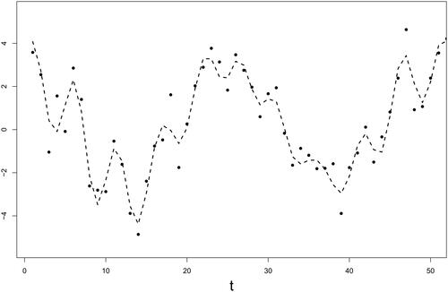
To demonstrate the effectiveness of the proposed method in capturing the underlying data structure, the sum of the two extracted eigen-sequences in Figures 5 and 6, respectively, is presented in Figure 7, which shows that the fitted curve characterizes the simulated data quite well. The proposed method also reveals that the observed data with noise come from two distinct components—one with a low frequency and the other with a high frequency.

Figure 7. Simulated Study III: comparing the simulated data (dots) and the fitted curve from the proposed adaptive sequential SSA (dashed line).

4.4. Real Data Analysis: Heart Rate Change Patterns Related to E-Cigarette Use

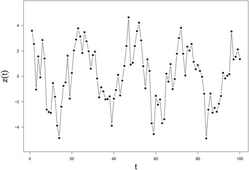
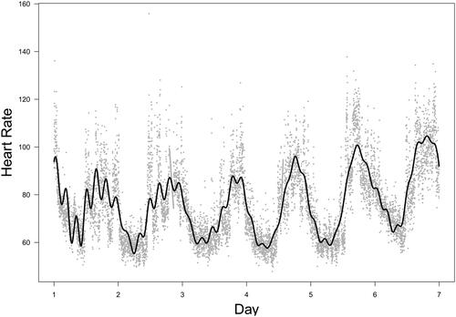
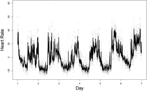
The methodological work presented in this paper was motivated by our experience with heart rate data collected from young adult e-cigarette users who wore Garmin Vivosmart 5 smartwatches (Garmin, Olathe, KS, USA) 24/7 for seven days. Participants also used the study app on their own smartphones to report e-cigarette use events during the 7 days. We utilized six full days of data measuring an e-cigarette user’s heart rate every minute to demonstrate an application of the proposed method. Figure 8 illustrates the observed heart rate data, with vertical dashed lines indicating the timings of vaping. As shown in this figure, there is substantial variation in heart rate in the neighborhood of any given time point.

Figure 8. Real data analysis: the observed heart rate data (dots) spanning 6 whole days; the vertical dashed lines indicate the timings of vaping events.

We adopted the conventional SSA approach to reconstruct the sequence, with the window length used to construct the Hankel matrix being half of the observed sequence. After performing SVD on the derived Hankel matrix, the first singular value is ${\sigma }_1=33341.$ However, ${\sigma }_1^2$ only constitutes 26% of the total variation. If we select eigentriples such that ${\sum }_{i=1}^k{\sigma }_i^2/{\sum }_{i=1}^w{\sigma }_i^2>0.9,$ the resulting value of k is 589. Thus, the conventional SSA under this criterion would need to select 589 eigentriples to reconstruct the sequence. Since the first two singular values account for 50% of the total variation and the third singular value constitutes only 3.8%, each of the rest eigentriples contains very little information for the reconstructed signal. For this reason, we used the first ten eigentriples (instead of 589) to reconstruct the signal. As shown in Figure 9, this reconstructed sequence is very smooth, whereas the participant’s heart rate exhibits significant variation especially during daytime. Such failure to capture the variation across daytime activities may result in loss of valuable information such as vaping behavior.

Figure 9. Real data analysis: the fitted curve using the conventional SSA method with the window length being equal to the half of the sequence and the first 10 eigentriples used for reconstruction (solid line) and the observed heart rate data (dots).

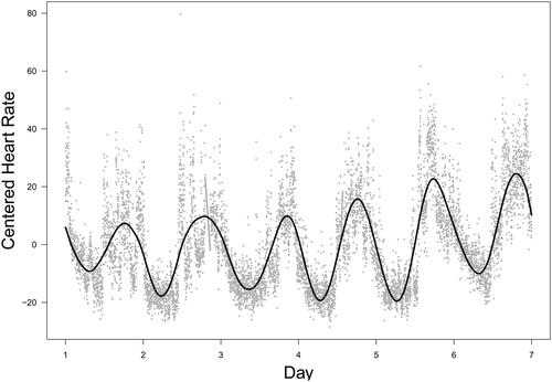
For the purpose of methodological comparison, the proposed method was also applied to the same set of heart rate data. The initial window length was estimated to be 781 that closely aligns with half-day measurements in the data set. The eigen-sequence extracted at this window length is depicted in Figure 10, alongside the heart rate centered by its sample mean. This figure indicates that the first eigen-sequence likely represents the average daily heart rate change pattern. The patterns on the first four days appear similar, whereas the patterns on the last two days are elevated compared to the preceding days.

Figure 10. Real data analysis: the first eigen-sequence (solid line) and the observed centered heart rates (dots).

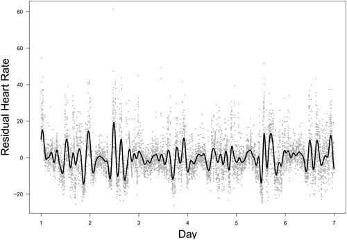
The proposed method next used the residual heart rate, which was calculated by subtracting the first eigen-sequence from the centered heart rate, to adjust the window length to 145 (approximately 2.4 h). The resulting second eigen-sequence, along with the residual heart rate, are plotted in Figure 11. This figure highlights that the second signal captures detailed variation within the range of hours.

Figure 11. Real data analysis: the second eigen-sequence (solid line) and the observed residual heart rate (dots).

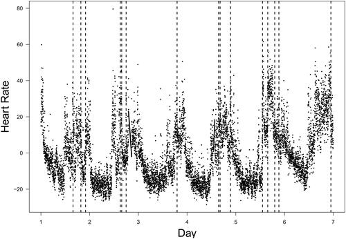
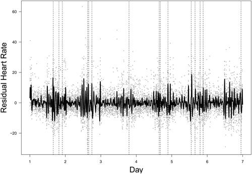
The proposed method continued to follow the algorithm and extracted the third eigen-sequence based on a window length of 46 which is shown in Figure 12. This eigen-sequence illustrates sharp changes in heart rate over short periods, especially around reported times of vaping events as indicated by the vertical lines. The peaks and troughs in the third eigen-sequence that manifest rapid fluctuations in heart rate are likely associated with the physiological effects of vaping.

Figure 12. Real data analysis: the third eigen-sequence (solid line) and the observed residual heart rate (dots).

The eigen-sequence extraction procedure was iterated until five eigen-sequences were generated, when the standard deviation of the residual sequence was less than 10% of the standard deviation of the original heart rate series. The sum of these five eigen-sequences and the centered heart rate are displayed in Figure 13, illustrating that heart rate decreases from the onset of sleep and increases upon waking up. In addition, heart rate variation is more pronounced during waking time compared to sleeping time.

Figure 13. Real data analysis: the fitted curve using the proposed adaptive sequential SSA (solid line) and the observed heart rate data (dots).

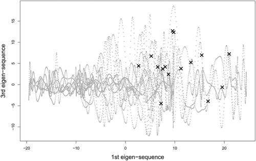
We also investigated heart rate change patterns that may be related to vaping events by plotting the scatter plots of pairwise eigen-sequences. The scatter plot of the first and the third eigen-sequences in Figure 14 shows that the majority of vaping events occur when the first and the third eigen-sequences are both positive values. Because the first eigen-sequence, as demonstrated in Figure 10, is likely to reflect the average, a positive value indicates that the heart rate around a vaping event is higher than the usual level. The positive value of the third eigen-sequence further characterizes the drastic change after vaping as demonstrated in Figure 12. These findings are, in general, consistent with previous studies Chaumont et al. (2018); Garcia et al. (2020); Tsai et al. (2020). A very small number of points in Figure 14 that have negative values of the third eigen-sequence may reflect those situations when there was a delay in reporting (i.e. the effect of e-cigarette use was wearing off).

Figure 14. Real data analysis: a scatter plot of the first and third eigen-sequences (dots); time stamps of vaping events are marked with ×.

Compared to the conventional SSA method, our proposed method may appear time-consuming because it requires conducting SVD at each window length during the first step of window length estimation. However, the proposed algorithm only requires calculating truncated SVD that can be efficiently carried out by widely available algorithms such as the Lanczos algorithm Larsen (1998) or Arnoldi method Lehoucq et al. (1998) implemented in ARPACK. To benchmark the proposed method’s computational performance compared to the conventional SSA method, we recorded the execution time on our computer equipped with an Intel(R) Xeon(R) CPU E3-1505M v6 @ 3.00 GHz, 3000 Mhz, 4 Core(s), 8 Logical Processors, and 64 GB RAM, under Microsoft Windows 10 Home edition. The Julia programming language Bezanson et al. (2017), version 1.9.3, was used to implement both methods. The result shows that the computational efficiency of the proposed method (54 s) is comparable to the conventional method (51 s).

4.5. Simulation Study IV: The Reconstructed Heart Rate Data

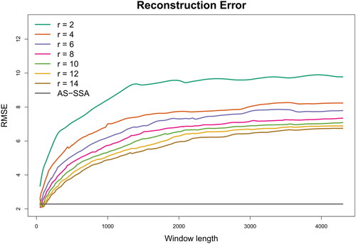
To compare the proposed method with the conventional SSA in terms of reconstruction errors under a real-world scenario, we utilized the reconstructed series from Section 4.4 as the true time series (see the fitted curve in Figure 13). To generate simulated data with the same length as the real data (8,638 data points), we introduced white noise from a normal random variable distribution, with a mean of zero and a standard deviation of 5.13 (estimated from the data). The resulting data were analyzed by both the proposed method and the conventional SSA with various window lengths (from 50 to 4,300 with an increment of 5) and numbers of groups (from 2 to 14). For each configuration, the root mean square error (RMSE), calculated as the root mean square difference between the reconstructed series and the true series, was used to measure the reconstruction error.

Figure 15 shows reconstruction errors under different combinations of window length and number of groups. Almost all RMSE values based on the conventional SSA are larger than the error based on the proposed AS-SSA method, which reconstructed the series after five iterations and resulted in RMSE = 2.29, as depicted by the horizontal line at the bottom of Figure 15. The RMSE of the conventional SSA method is slightly smaller than that of the proposed method only when the window length is small (window length = 50). These results indicate that the proposed adaptive approach outperforms conventional approaches for most window length selections, all of which rely on a single window length.

Figure 15. Simulated Study IV: the reconstruction error measured by RMSE (y-axis) based on the proposed adaptive sequential SSA (AS-SSA) and the conventional SSA with various window lengths (x-axis) and numbers of groups (r). The true time series was reconstructed from real heart rate data using the proposed AS-SSA method.

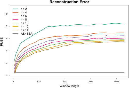
To investigate the possibility that the above simulation could potentially favor the AS-SSA method, we conducted another set of simulation using the conventional SSA method to derive the true time series. Specifically, we applied the conventional SSA with a window length of 100 to extract heart rate patterns. By evaluating the singular values in the trajectory matrix, we found that the first 22 singular values captured 90% of the total variation. These singular values were thus used to derive the denoised heart rate, which was treated as the true time series. The same white noise with a mean of zero and a standard deviation of 5.13 was then added to generate simulated data. Both the conventional SSA and the proposed AS-SSA methods were applied to analyze the simulated data. The reconstruction errors (RMSE) for the SSA across different combinations of window length and number of groups are shown in Figure 16, with the horizontal line indicating the RMSE (2.44) corresponding to the AS-SSA that reconstructed the series after five iterations.

Figure 16. Simulated Study IV: the reconstruction error measured by RMSE (y-axis) based on the proposed adaptive sequential SSA (AS-SSA) and the conventional SSA with various window lengths (x-axis) and numbers of groups (r). The true time series was reconstructed from real heart rate data using the conventional SSA with the window length being 100 and the number of groups being 22.

The results of the simulation using the true time series reconstructed by the conventional SSA (Figure 16) are compared with those of the simulation based on the AS-SSA reconstructed series (Figure 15) to evaluate whether the results could be influenced by the way the true time series was generated. Both figures actually show the same story: the proposed AS-SSA method consistently achieved the smallest reconstruction error across a variety of scenarios; the conventional SSA method had a slightly smaller reconstruction error only under rare conditions with very small window length (e.g. 50) and a large number of groups (r = 12, 14). Moreover, the proposed AS-SSA method only enjoyed a small advantage when the true time series was simulated based on the AS-SSA method (RMSE = 2.29), compared to when the series was simulated using the conventional SSA method (RMSE = 2.44). Overall, the simulation results did not change with the way the true time series was generated.

In addition to the main finding of the proposed method’s effectiveness in achieving the smallest reconstruction error, there are some interesting findings from Simulation Study IV. Contrary to the commonly adopted recommendation of using large window lengths Golyandina (2010), Figures 15 and 16 show that the reconstruction error increases with the window length when the number of groups is fixed. Although the difference in RMSE between large window lengths (e.g. 4,300, close to half of the series length) and smaller ones (e.g. 2,000, close to one-fourth of the series length) is relatively small, the computation time significantly increases with larger window lengths, particularly for very long time series. Thus, adopting a large window length may not produce the kind of benefit that one may expect. Figures 15 and 16 also indicate that for any fixed window length, RMSE decreases as the number of groups increases. Because the true time series comprises five eigen-sequences, theoretically speaking, 10 groups should be sufficient. Yet, utilizing r = 14 yields a smaller RMSE, indicating that there is still information not accounted for beyond r = 10. This implies that one fixed window length may not universally fit all eigen-sequences well.

5. Conclusion and Discussion

The methodological work conducted in this study could potentially advance future research and intervention in the nicotine and tobacco filed. The real data analysis on 6-day heart rate data from a young adult e-cigarette user demonstrates that vaping events did not manifest randomly in the scatter plot of the pair of eigen-sequences. Instead, they clustered within a confined region of the scatter plot. This opens up an opportunity for scientists to effectively identify the high-risk periods for individual e-cigarette users so intervention messages could be tailored to each person’s unique vulnerability. The proposed adaptive sequential approach also ensures that the window length is tailored to the specific heart rate change patterns of individual users. Furthermore, although prior research has identified lower resting heart rate variability as a marker for substance users’ compromised ability to regulate cognitive, behavioral, and emotional responses to stress Wieman and Eddie (2022)—an important precursor for substance use behavior—the proposed method could provide a more fine-grained analysis of individual heart rate change patterns. Such analysis may facilitate addiction scientists’ understanding of the progression of nicotine use disorder by examining the difference in this” digital biomarker” across e-cigarette users with various levels of nicotine dependence. All of these possibilities that the proposed method has created for the field could have significant impact on public health as we combat the vaping epidemic among the youth and young adult population in the U.S.

While it is well-known that a time series with a sinusoidal function’s frequency yields two prominent singular values in the derived Hankel matrix, we demonstrated that this pair of singular values indeed depend on the chosen window length in SSA. The conventional method that recommends using a larger window length performs well for time series with a short to moderate size. Yet, for considerably lengthy time series such as heart rate data, this approach becomes excessively time-consuming because it involves massive computation of SVD for a large matrix. Using a large window length also amplifies the mean squared reconstruction error. To fill this critical gap in the methodology literature, this study has provided an adaptive sequential SSA method to iteratively choose an optimal window length so that important eigen-sequences (i.e. signals) can be extracted efficiently with minimal reconstruction error. Importantly, this proposed method can handle not only short-moderate time series but also long time series.

Conventional SSA does not necessitate the time series to be mean-centered. Yet, our experience with heart rate data revealed that if non-centered (i.e. observed) data were used in the analysis, the first singular value of SSA would account for more than 99% of the total variation. In other words, only one rank-one matrix would be selected to extract sequences, resulting in possible loss of structural details in the time series. This phenomenon was also discussed by Wall et al. (2003). As demonstrated by the real data analysis, after the heart rate data were centered by the sample mean, the details of heart rate variation became discernible.

Our proposed method opens avenues for future research. One compelling area is the evaluation of the eigen-sequences against true sequences. Given the fundamentally non-parametric nature of our approach, expressing the eigen-sequences using a parametric form could be challenging. Another area is related to our assumption that the time series can be expressed as a sum of sinusoidal functions with various frequencies. As a result of the assumption, when the time series is not periodic, the proposed method tends to select a long window length. Thus, future work on developing a technique to address this situation is warranted.

Acknowledgment

The content is solely the responsibility of the authors and does not necessarily represent the official views of the NIH. The authors declare no conflict of interest.

Disclosure Statement

No potential conflict of interest was reported by the author(s).

Additional information

Funding

This research was supported by a grant funded by the National Institutes of Health (NIH): R01 DA049154 to A. Buu.

References

- Atikur Rahman Khan M, Poskitt DS. 2013. A note on window length selection in singular spectrum analysis. Aus NZ J of Statistics. 55(2):87–108.
- Bezanson J, Edelman A, Karpinski S, Shah VB. 2017. Julia: a fresh approach to numerical computing. SIAM Rev. 59(1):65–98.
- Broomhead DS, King GP. 1986. Extracting qualitative dynamics from experimental data. Physica D. 20(2-3):217–236.
- Broomhead DS, King GP, et al. 1986. On the qualitative analysis of experimental dynamical systems. Nonlinear Phenomena and Chaos. 113:114.
- Chaumont M, de Becker B, Zaher W, Culié A, Deprez G, Mélot C, Reyé F, Van Antwerpen P, Delporte C, Debbas N. 2018. Differential effects of e-cigarette on microvascular endothelial function, arterial stiffness and oxidative stress: a randomized crossover trial. Sci Rep. 8(1):10378.
- Cong F, Zhong W, Tong S, Tang N, Chen J. 2015. Research of singular value decomposition based on slip matrix for rolling bearing fault diagnosis. J Sound Vib. 344:447–463.
- de Prony GR. 1795. Essai experimental et analytique: sur les lois de la dilatabilite des fluides elastique et sur celles de la force expansive de la vapeur de l’eau et de la vapeur de l’alkool, a differentes temperatures. Journal Polytechnique ou Bulletin du Travail Fait a L’Ecole Centrale Des Travaux Publics. 1(22):24–76.
- Garcia PD, Gornbein JA, Middlekauff HR. 2020. Cardiovascular autonomic effects of electronic cigarette use: a systematic review. Clin Auton Res. 30(6):507–519.
- Golyandina N. 2010. On the choice of parameters in singular spectrum analysis and related subspace-based methods. arXiv preprint arXiv:1005.4374.
- Golyandina N, Korobeynikov A, Zhigljavsky A. 2018. Singular spectrum analysis with r. Berlin, Heidelberg: Springer.
- Golyandina N, Nekrutkin V, Zhigljavsky AA. 2001. Analysis of time series structure: SSA and related techniques. Boca Raton, Florida: CRC press.
- Golyandina N, Zhigljavsky A. 2020. Singular spectrum analysis for time series (2nd ed.). Berlin, Germany: Springer.
- Guo M, Li W, Yang Q, Zhao X, Tang Y. 2020. Amplitude filtering characteristics of singular value decomposition and its application to fault diagnosis of rotating machinery. Measurement. 154:107444.
- Hassani H, Mahmoudvand R, Zokaei M. 2011. Separability and window length in singular spectrum analysis. CR Math. 349(17-18):987–990.
- Khan MAR, Poskitt D, et al. 2010. Description length based signal detection in singular spectrum analysis. Monash Econometrics and Business Statistics Working Papers. 13(10):1–35.
- Khan MAR, Poskitt DS. 2011. Window length selection and signal-noise separation and reconstruction in singular spectrum analysis. Australia: Department of Econometrics and Business Statistics, Monash University.
- Knapik T, Ratiarison A, Razafindralambo H. 2022. An experimental evaluation of choices of ssa forecasting parameters.
- Larsen RM. 1998. Lanczos bidiagonalization with partial reorthogonalization. DPB. 27(537):70.
- Lehoucq RB, Sorensen DC, Yang C. 1998. Arpack users’ guide: solution of large-scale eigenvalue problems with implicitly restarted arnoldi methods. Philadelphia, Pennsylvania: SIAM.
- Ma H-G, Lei R, Kong X-Y, Liu Z-Q, Jiang Q-B. 2012. Determine a proper window length for singular spectrum analysis.
- Sanei S, Hassani H. 2015. Singular spectrum analysis of biomedical signals. Boca Raton, Florida: CRC Press.
- Sun M, Li X, et al. 2017. Window length selection of singular spectrum analysis and application to precipitation time series. Global NEST J. 19(2):306–317.
- Tsai M, Byun MK, Shin J, Crotty Alexander LE. 2020. Effects of e-cigarettes and vaping devices on cardiac and pulmonary physiology. J Physiol. 598(22):5039–5062.
- Unnikrishnan P, Jothiprakash V. 2019. Selection of window length in singular spectrum analysis of a time series. In Nonparametric statistics. Cham, Switzerland: Springer International Publishing. p. 311–322. https://doi.org/10.1007/978-3-319-96941-1_21
- Wall ME, Rechtsteiner A, Rocha LM. 2003. Singular value decomposition and principal component analysis. In A practical approach to microarray data analysis. Boston, Massachusetts: Springer, p. 91–109.
- Wang R, Ma H-G, Liu G-Q, Zuo D-G. 2015. Selection of window length for singular spectrum analysis. J Franklin Inst. 352(4):1541–1560.
- Wieman ST, Eddie D. 2022. OCT). Heart rate variability biofeedback for substance use disorder: health policy implications. Policy Insights from Behav Brain Sci. 9(2):156–163.
- Yang B, Dong Y, Yu C, Hou Z. 2016. Singular spectrum analysis window length selection in processing capacitive captured biopotential signals. IEEE Sensors J. 16(19):7183–7193.
- Zhao X, Ye B. 2019. Separation of single frequency component using singular value decomposition. Circuits Syst Signal Process. 38(1):191–217.