On stock returns volatility and trading volume of the nairobi securities exchange index

ABSTRACT

This study attempts to put forward a framework that can be utilized to model the dynamics of the underlying returns on asset. The intention is to probe the dynamic connection between volatility of stock returns and trading volume of the Nairobi Securities Exchange (NSE20) index. The consequence of incorporating trading volume in the equation for conditional variance of the generalized autoregressive conditional heteroscedasticity (GARCH) model on volatility persistence is investigated. Further, this study brings into play GARCH, GARCH-M, and EGARCH models conditioned to normal, student-t and generalized error distributions to model the dynamic structure of the NSE20 index for the period 2 January 2001 to 31 December 2017. The results disclose some well-known stylized facts of returns on stock, for instance, volatility clustering, heavy tails, leverage effects, and leptokurtic distribution. The estimates of parameters of the three models, that is, GARCH (1, 1), GARCH-M (1, 1), and EGARCH models report that the correlation between stock returns volatility and trading volume is positive and statistically significant. Moreover, estimates of the coefficients of EGARCH (1, 1) model report an increased measure of persistence on volatility as well as volatility asymmetry and the absence of leverage effect in the returned volatility. Also, the estimates of GARCH (1, 1) and GARCH-M (1, 1) parameters report that volatility persistence dwindles after trading volume is incorporated in the equation for the conditional variance.

Keywords:

• Stock returns
• trading volume
• volatility
• heteroscedasticity
• GARCH models

1 Introduction

In the previous financial modeling studies, the linkage between return, volatility and trading volume is a key issue since it provides insights into the microstructure of financial markets. Wiley and Daigler (1999) argue that the connection between price and volume can be attributed to the role played by information flow in the formation of price. Abbondante (2010) defines trading volume as: the amount of shares that are transacted on a daily basis and states that it is an imperative pointer in technical analysis since it is used to assess the worth of the price of stock which could either be increasing or decreasing.

The motivation of investors to trade is fundamentally contingent on their trading undertaking; it might be to conjecture on the information for the market or diversification of portfolios so as to spread risk, or as well the exigency for liquidity. These divergent reasons for doing business may be attributed to the interpretation of diverse information flow into the market. As a result, total amount of shares may start off from one of the investors holding diverse sets of information. Many studies have disclosed that the flow of information into the market is associated with the total amount of shares and volatility as revealed in the studies of, Gallant et al. (1992), Lamoureux and Lastrapes (1990), and He and Wang (1995) report that the price of stocks changes after a new information flows into the market and thus it can be argued that prices of stocks, volatility and total amount of shares are related.

Moreover, numerous studies suggest existence of a very strong connection between returns on stocks, volatility and trading volume across international markets as evidenced by the studies of Connolly and Wang (2003). It is thus rational to take into account the fact that recent international stock markets process continuous trading and uninterrupted information flow in their everyday market transactions, which is indicated by returns on stocks, volatility and volume, see Lee and Rui (2002).

The dynamic and contemporaneous connection between total shares traded and stock returns have been a foundation for empirical research. Lee and Rui (2002) established that trading volume is granger caused by returns on stock in the developed markets, that is, the US, UK, and Japan markets. In their study, De Medeiros and Doornik (2006), found a contemporaneous and dynamic association between returns volatility and total shares transacted for the stock market of Brazil. Mahajan and Singh (2009) report that total amount of shares transacted and volatility have a positive correlation. Their study further indicates a one-way causality, that is, from returns on stocks to total shares traded. More recently, Choi et al. (2012) in his study utilized GJR-GARCH and EGARCH models on stock market of Korea and reported that trading volume is a significant tool in the prediction of the volatility dynamics.

A lot of empirical and theoretical studies on the connection between price and trading volume have been carried out and they have reported a positive correlation between stock returns, volatility and trading volume, see Karpoff (1987). On the other hand, some of these studies for the different stock markets have reported varied results about the causal connection between price and volume despite the fact that many findings have established that the contemporaneous correlation between trading volume and returns is positive.

In their study, Lamoureux and Lastrapes (1990) argue that movement of price is caused by the random flow of information into the market and that this movement leads to trading volume changes. Trading volume can be utilized as a proxy variable despite the fact that the flow of information cannot be observed and thus using trading volume as an explanatory variable for heteroscedasticity of return series will lead to heteroscedasticity of variability of return series being absorbed. Therefore, if trading volume is incorporated in the GARCH model it may cause both the ARCH and GARCH effects, which represent volatility persistence, to reduce or even vanish. Furthermore, Lamoureux and Lastrapes (1990) reveal that conditional variance persistence disappears after a latent variable, that is, trading volume, is introduced in the conditional variance equation. The work of Omran and McKenzie (2000) and Miyakoshi (2002) examined the stock market of Australia and Tokyo stock exchange, respectively, and documented analogous results to that of Lamoureux and Lastrapes (1990). On the other hand, a research by Miyakoshi (2002) utilized the daily prices and volumes of treasury bonds future markets and reported that GARCH effects persisted even after trading volume was added in the conditional variance equation. Studies of Darrat et al. (2003), among others, corroborate this evidence.

Numerous studies are in agreement that trading volume contributes significantly to the time series return process. As such, McKenzie and Faff (2003) have disclosed that the conditional autocorrelation in returns on stocks is to a great extent reliant on total shares transacted for individual stocks but not for the index, implying the fact that liquidity disparities for stocks has a remarkable impact at individual level but not at aggregate level. Brailsford (1996), utilizing Australian equities, has disclosed a considerable decrease in volatility persistence after using trading volume as a proxy for the rate of information flow. In contrast, the studies of Ahmed et al. (2005), Huang and Yang (2001), Salman (2002), Yüksel (2002), and Chen et al. (2001) have generally reported that persistence in return volatility remains even after volume is integrated in conditional variance equation.

Although an extensive research into the aspects of return volatility and total shares transacted is widely reported, most of the studies have been done based on the developed stock markets and hence inadequate similar literature exists in emerging markets. Moreover, studies on whether volatility persistence reduces or completely disappears after including trading volume into the conditional variance of GARCH model have reported conflicting results. As a consequence, the main objective of this study is proposing a general framework that will model the dynamics of the underlying asset returns, incorporating some known stylized facts often observed in different financial time series such as volatility clustering, heavy tails, leverage effects, leptokurtic distribution among others. This framework will be utilized to investigate the contemporaneous and dynamic connection between return on stock volatility and total shares transacted in an emerging stock market (the Nairobi Securities Exchange). Furthermore, the study examines the effect of integrating trading volume into the conditional variance equation of the generalized autoregressive conditional heteroscedasticity (GARCH) models on volatility persistence. Statistical models that have been previously utilized to model financial time series are applied in this study, and each model is conditioned to normal, student-t, and generalized error distributions, that is, GARCH(1,1),GARCH-M(1,1), and EGARCH(1,1) models are utilized. As a consequence, this study contributes to the growing literature, and gives insight about the micro-structure of the Nairobi Securities Exchange by modeling the dynamics of stock return volatility and its correlation with trading volume of the NSE20 index.

The rest of this research article is organized as follows: Section 2 describes the ARCH and GARCH-type models that are used to model the log returns and volume along with the data used by the study. Section 3 provides the descriptive statistics, the general results and discussion of the findings of the study. Finally, section 4 concludes the article.

2 Methodology

2.1 Modelling the underlying asset

Consider a stochastic process,$(X_t{)}_{t\ge 0}$, on a probability space $(\mathrm{\Omega },\mathcal{F},{\mathcal{F}}_{t\in [0,T]},\mathbb{P})$ describing the uncertainity of the stock market. $\mathbb{P}$ is the physical probability measure and ${\mathcal{F}}_t$ is a filtration representing all the information set upto time $t-1$. Suppose that $S_t$ is the stock price at time $t$ adapted to the filtration ${\mathcal{F}}_t$ and $X_t$ is the continously compounded stock return, then the following definition can be made.

Definition 2.1 Let $X_t$ be a random variable whose mean and variance are conditional on the information set ${\mathcal{F}}_{t-1}$ containing all the information upto time $t-1$. Then the model for the asset returns under measure $\mathbb{P}$ is defined as

(1) $\begin{array}{ccc}{X}_t=ln(\frac{S_t}{S_{t-1}}|{\mathcal{F}}_{t-1})& \hspace{0.17em}& \hspace{0.17em}\\ X_t=\mathbb{E}[(X_t|{\mathcal{F}}_{t-1})]+r_t,r_t={\sigma }_t{\epsilon }_t& \hspace{0.17em}& \hspace{0.17em}\\ {\sigma }_t^2=\mathbb{E}[(X_t-\mathbb{E}[X_t|{\mathcal{F}}_{t-1}{])}^2|{\mathcal{F}}_{t-1}]& \hspace{0.17em}& \hspace{0.17em}\\ {\epsilon }_t\sim i.i.d(0,1)implyingthat{r}_t|{\mathcal{F}}_{t-1}\sim \mathbb{D}(0,{\sigma }_t)& \hspace{0.17em}& \hspace{0.17em}\end{array}$(1)

where $\mathbb{D}$ stands for the distribution that is assumed to be either normal or leptokurtic (students-t and GED), ${\mu }_t$ denote the conditional mean,${\sigma }_t$ denote the conditional variance and $r_t$ is mean-corrected asset return.

2.2 ARCH model

Engle (1982) showed that the serial correlation in squared returns, or conditional heteroskedasticity, can be modeled using an autoregressive conditional heteroskedasticity (ARCH) model of the form

(2) $\begin{array}{ccc}{X}_t={\mathbb{E}}_{t-1}[X_t]+r_t,r_t={\sigma }_t{\epsilon }_t,{\sigma }_t^2=\omega +{\sum }_{i=1}^p{\alpha }_i{r}_{t-p}^2& \hspace{0.17em}& \hspace{0.17em}\end{array}$(2)

where ${\mathbb{E}}_{t-1}[.]$ represents expectation conditional on information available at time $t-1$, and ${\epsilon }_t$ is a sequence of independent and identically distributed(i.i.d) random variables with mean zero and unit variance. The parameter restrictions, $\omega \ge 0,{\alpha }_i\ge 0$ for $i=1,...,p$ and ${\alpha }_p>0$ are required for positivity of the conditional variance,${\sigma }_t^2$.

2.3 GARCH model

We utilize the GARCH model, which is a generalization of the ARCH model developed by Engle (1982), to investigate the effect of trading volume on stock return volatility. The model is characterized by its ability to capture volatility clustering, and it is widely used to account for non-uniform variance in timeseries data. The general GARCH(p,q) model is defined as;

(3) $r_t={\sigma }_t{\epsilon }_t,{\sigma }_t^2=\omega +\sum _{i=1}^p{\alpha }_i{r}_{t-i}^2+\sum _{j=1}^q{\beta }_j{\sigma }_{t-j}^2$(3)

where q is the GARCH degree; p is the ARCH process degree,${\epsilon }_t$ is a sequence of independent and identically distributed(i.i.d) random variables with zero mean and variance 1, that is, $\omega >0,{\alpha }_i\ge 0,{\beta }_j\ge 0$ and ${\sum }_{i=1}^p{\alpha }_i+{\sum }_{j=1}^q{\beta }_j<1$. The term,${\sigma }_t$,is the volatility process of the returns, $X_t$, which should be positive and depend on the past innovations ${\epsilon }_{t-1}$, that is, ${\sigma }_t$ should be measurable with respect to the $\sigma$-algebra generated by ${\epsilon }_{t-1}$. The constraint ${\sum }_{i=1}^p{\alpha }_i+{\sum }_{j=1}^q{\beta }_j<1$ implies that the unconditional variance of $X_t$ is finite, whereas its conditional variance,${\sigma }_t^2$, evolves over time. We note that the basic and widely used model is GARCH(1,1) which is expressed as

(4) $r_t={\sigma }_t{\epsilon }_t,{\sigma }_t^2=\omega +{\alpha }_1{r}_{t-1}^2+{\beta }_1{\sigma }_{t-1}^2$(4)

In equation (3)(3) $r_t={\sigma }_t{\epsilon }_t,{\sigma }_t^2=\omega +\sum _{i=1}^p{\alpha }_i{r}_{t-i}^2+\sum _{j=1}^q{\beta }_j{\sigma }_{t-j}^2$(3) above, $X_t$ is the daily rate of returns, $\omega$ is the non-changing variance that corresponds to the long-run average, ${\alpha }_1$ represents the first-order ARCH term which broadcasts information pertaining volatility from an earlier period, and ${\beta }_1$, is the first-order GARCH term, which is the new information that was not available at the time the previous forecast was made. If the parameters ${\alpha }_1$ and ${\beta }_1$ are greater than 1, the shocks to volatility does not die off over time. The magnitude of these parameters determines the extend of volatility persistence. The closer the sum of ${\alpha }_1$ and ${\beta }_1$ to 1, the more the shocks to volatility does not die off.

2.3.1 Conditional mean specification

To capture autocorrelation caused by market microstructure effects on non-trading effects, the conditional mean ${\mathbb{E}}_{t-1}[X_t]$ is typically specified as a constant or possibly a low order autoregressive-moving average (ARMA) process, however, this is dependent on the frequency of the data and type of asset. Incase of extreme or unusual market events have happened during sample period, then dummy variables associated with these events are often added to the conditional mean specification to remove these effects. Therefore, the typical conditional mean specification is of the form

(5) $E_{t-1}[X_t]=\omega +{\sum }_{i=1}^p{\varphi }_i{X}_{t-i}+{\sum }_{j=1}^q{\theta }_j{r}_{t-j}+{\sum }_{m=1}^M{\beta }^{\prime }m{Y}_{t-m}+r_t$(5)

where $Y_t$ is a $kx1$ vector of explanatory variables and $k$ is the length of the sample used.

2.3.2 Explanatory variables in the conditional variance

Exogenous variables can be added to the conditional GARCH(p,q) formula just as in a similar manner they are added in the conditional mean equation as follows

(6) $r_t={\sigma }_t{\epsilon }_t,{\sigma }_t^2=\omega +{\sum }_{i=1}^p{\alpha }_i{r}_{t-i}^2+{\sum }_{j=1}^q{\beta }_j{\sigma }_{t-j}^2+{\sum }_{m=1}^M\delta {\prime }_m{Z}_{t-m}$(6)

where $Z_t$ is a $kx1$ vector of random variables, and $\delta$ is a $kx1$ vector of positive coefficients. These coefficients, for instance, trading volume, microeconomic news announcements, help predict volatility, see Gallant et al. (1992).

In financial market, high risk is often associated with high returns. Although the current capital asset pricing theory does not reflect such a simple correlation, it does suggest existence of some interactions between risk (as measured by volatility) and the expected returns. In his work, Engle et al. (1987) extended the fundamental GARCH model so that the conditional volatility can generate a risk premium which is part of the expected returns. The extended GARCH model is referred to as GARCH-in-mean, or denoted as GARCH-M.

2.4 The GARCH-M model

In finance, return of a stock could be dependent on its volatility. This phenomenon can be best modelled using GARCH in mean model written as GARCH-M. A simple GARCH-M(1,1) model is of the form

(7) $X_t={\mathbb{E}}_{t-1}[X_t]+{\lambda }_1{\sigma }_t^2+r_t,\mathrm{w}\mathrm{h}\mathrm{e}\mathrm{r}\mathrm{e},r_t={\sigma }_t{\epsilon }_t,\mathrm{a}\mathrm{n}\mathrm{d}{\sigma }_t^2=\omega +{\alpha }_1{r}_{t-1}^2+{\beta }_1{\sigma }_{t-1}^2$(7)

where $X_t$ and $r_t$ are the log return and the mean-corrected log return series, respectively. The coefficient ${\lambda }_1$ is the risk premium and if its value is positive, then the implication is that the stock return has a positive correlation with its previous volatility.

2.5 The exponential GARCH (EGARCH) model

This model captures asymmetric responses of time-varying variance to shocks and, at the same time, ensures that the variance is always positive. The general EGARCH(p,q) model is defined as

(8) $ln({\sigma }_t^2)=\omega +\sum _{i=1}^p\{{\alpha }_i([|r_{t-i}|-\mathbb{E}|r_{t-i}|])+{\gamma }_i{r}_{t-i}\}+\sum _{j=1}^q{\beta }_{j}ln({\sigma }_{t-j}^2)$(8)

where ${\gamma }_i$ is the parameter that gives response to asymmetry which is also referred to as the leverage parameter. The value of ${\gamma }_i$ is expected to be greater than 1 in most empirical situations so that volatility into the future or uncertainty can be increased by a negative shock while a positive shock reduces the effect on future uncertainty. The parameter ${\beta }_j$ is a measure of volatility persistence such that if the value is close to one, then volatility persists for a long time. In financial market analysis, a negative shock mostly implies bad news which leads to a more unpredictable future. As a result, for instance, investors would require higher returns from stocks to compensate for taking the increased risk in their investment. In this study, we employ EGARCH(1,1) model defined as follows;

(9) $ln({\sigma }_t^2)=\omega +\{{\alpha }_1([|r_{t-1}|-\mathbb{E}|r_{t-1}|])+{\gamma }_1{r}_{t-1}\}+{\beta }_{1}ln({\sigma }_{t-1}^2)$(9)

2.6 Conditional distributions

We present the distributions that are used here to model the financial log returns as follows. Each distribution is standardized to have a zero mean and a unit variance.

2.6.1 Normal distribution

Let $f(r_t|{\mathcal{F}}_{t-1})$ be a conditional distribution which is normally distributed with mean ${\mu }_t$ and variance ${\sigma }_t^2$, then the likelihood function of $f(r_t|{\mathcal{F}}_{t-1})$ is given by

(10) $f(r_1,\dots .,r_T;\theta )=f(r_1;\theta )\prod _{t=2}^T\frac{1}{\sqrt{2\pi {\sigma }_t^2}}exp[-\frac{{(r_t-{\mu }_t)}^2}{2{\sigma }_t^2}]$(10)

Here,$f(r_1;\theta )$ is the marginal density function of the initial observation,$r_1$. The value of $\theta$ that maximizes equation (10)(10) $f(r_1,\dots .,r_T;\theta )=f(r_1;\theta )\prod _{t=2}^T\frac{1}{\sqrt{2\pi {\sigma }_t^2}}exp[-\frac{{(r_t-{\mu }_t)}^2}{2{\sigma }_t^2}]$(10) is the maximum likelihood estimate of $\theta$ given by

(11) $L=lnf(r_1,\dots .,r_T;\theta )=lnf(r_1;\theta )-\frac{1}{2}\sum _{t=2}^T[ln2\pi +ln{\sigma }_t^2+\frac{{(r_t-{\mu }_t)}^2}{{\sigma }_t^2}]$(11)

2.6.2 Student-t distribution

Let $x_v$ be a student-t distribution with $v$ degrees of freedom, then $Var(x_v)=v/(v-2)\mathrm{f}\mathrm{o}\mathrm{r}v>2$. If we define ${\epsilon }_t=x_v/\sqrt{v/(v-2)}$,then the probability density function of ${\epsilon }_t$ is

(12) $f({\epsilon }_t|v)=\frac{\mathrm{\Gamma }(v+1)/2}{\mathrm{\Gamma }(v/2)\mathrm{\Gamma }(v-2)\pi }[1+\frac{{\epsilon }_t^2}{v-2}{]}^{-(1+v)/2},v>2$(12)

where $\mathrm{\Gamma }(x)={\int }_0^{\mathrm{\infty }}{y}^{x-1}{e}^{-x}dy$ is a Gamma function. Further, if we let $r_t={\sigma }_t{\epsilon }_t$, then the conditional likelihood function of $r_t$ is given by

(13) $\begin{array}{rl}& f(r_{m+1},\dots .,r_T|\alpha ,A_m)={\prod }_{t=m+1}^T\frac{\mathrm{\Gamma }((v+1)/2)}{\mathrm{\Gamma }(v/2)\sqrt{(v-2)\pi }}\\ & \frac{1}{{\sigma }_t}[1+\frac{r_t^2}{(v-2){\sigma }_t^2}{]}^{(v+1)/2}\end{array}$(13)

where $v>2$ and $A_m=(r_1,\dots ,r_m)$.

For specified degrees of freedom $v$ of student-t distribution, the conditional log-likelihood function is given by

(14) $L=ln(r_{m+1},\dots \dots .,r_T|\alpha ,A_m)=-\sum _{t=m+1}^T[\frac{v+1}{2}ln(1+\frac{r_t^2}{(v-2){\sigma }_t^2})+\frac{1}{2}ln{\sigma }_t^2]$(14)

2.6.3 The generalized error distribution(GED)

The likelihood function for the GED is given by

(15) $f(r_t,{\mu }_t,{\sigma }_t,v)=\frac{v{e}^{-\frac{1}{2}|\frac{r_t-{\mu }_t}{{\sigma }_t\lambda }{|}^v}}{\lambda 2^{(1+1/v)}\mathrm{\Gamma }(1/v)},1<r_t<\mathrm{\infty },\mathrm{w}\mathrm{h}\mathrm{e}\mathrm{r}\mathrm{e}\lambda =[\frac{\mathrm{\Gamma }(1/v)}{4^{(1/v)}\mathrm{\Gamma }(3/v)}{]}^{1/2}$(15)

The likelihood function,i.e,equation 15(15) $f(r_t,{\mu }_t,{\sigma }_t,v)=\frac{v{e}^{-\frac{1}{2}|\frac{r_t-{\mu }_t}{{\sigma }_t\lambda }{|}^v}}{\lambda 2^{(1+1/v)}\mathrm{\Gamma }(1/v)},1<r_t<\mathrm{\infty },\mathrm{w}\mathrm{h}\mathrm{e}\mathrm{r}\mathrm{e}\lambda =[\frac{\mathrm{\Gamma }(1/v)}{4^{(1/v)}\mathrm{\Gamma }(3/v)}{]}^{1/2}$(15) above is maximized by

(16) $L=ln(\frac{v}{\lambda })-\frac{1}{2}|\frac{r_t-{\mu }_t}{{\sigma }_t\lambda }{|}^v-(1+1/v)ln2+ln[\mathrm{\Gamma }(1/v)]$(16)

If $v=2$, the GED yields the normal distribution. Also if $v<1$, the density function has thicker tails than the normal density function, whereas for $v>2$, it has thinner tails.

2.7 Empirical data

This study focuses on the daily stock index and trading volume as reported in Nairobi Securities Exchange for NSE20 share index for the period 1 January 2001 to 31 December 2017. The daily continuously compounded index returns and trading volume are calculated in terms of logarithmic change as follows: $X_t=ln[P_t/P_{t-1}]$ where $P_t$ and $P_{t-1}$ represents the daily closing index at day $t$ and day $t-1$ respectively. Similarly, differenced trading volume, $T_v$, is computed as $T_v=ln[V_t/V_{t-1}]$ where $V_t$ and $V_{t-1}$ is the trading volume at day $t$ and day $t-1$ respectively.

3 Results and discussion

3.1 Descriptive statistics

Table 1 reports some basic statistical properties of the data together with the Jarque-Bera test for normality. It is clearly seen that the mean for returns and trading volume are positive but close to zero. The returns and trading volume of NSE20 index have positive skewness; however, the excess kurtosis of returns exceeds 3 unlike that of volume which is less than 3 which means that the distributions of both series are right skewed and leptokurtic. The two series have heavy tails and show a strong departure from normality since the skewness and kurtosis are all statistically different from those of the normal distribution which are 0 and 3, respectively. The JB statistics clearly fails to accept the null hypothesis of normality for both returns and volume.

Table 1. Basic statistics for stock returns and trading volume

Data	Min	Max	Mean	Var	Std dev.	Skew	Ex.Kurt	JB
Returns	−0.08602	0.08634	0.00016	0.00007	0.00857	0.39295	8.32209	22,949***
Volume	−3.59679	3.84070	0.00103	0.61150	0.78199	0.09298	−0.77628	888***

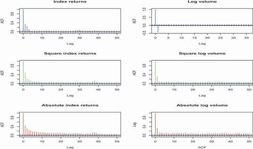
Figure 1 shows a graphic display of stock prices, index returns, squared index returns, and absolute index returns of NSE20 index along with trading volume, log volume, squared log volume, and absolute log volume. Clearly, the stock prices are not stationary, but the same cannot be said for trading volume. However, the index returns and logs of the trading volume series appears stationary. Also, the log returns do not display a clear noticeable pattern of behavior, but there is some persistence implied by the plots of the squared and absolute returns which represent the returns volatility. Precisely, volatility clustering is evident from the plots, that is, small volatility values are followed by small values and large volatility values are followed by large values. A confirmation of this behavior is shown in Figure 2 which displays the sample autocorrelations of the two series. There is no clear evidence of serial correlation from the log returns and log volume, but the squared and absolute returns as well as squared log volume and absolute log volume are positively auto-correlated. Also, the decay rates of the sample autocorrelations of $X_t$,$X_t^2$,$|X_t|$,$T_v$,$T_v^2$,$|T_v|$ appear much slower which perhaps suggests long memory behavior.

Figure 1. Returns, squared returns and absolute returns for NSE20 index and volume

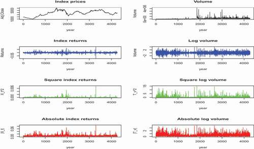
Figure 2. Acf for daily NSE20 index and volume

3.2 Empirical findings and discussion

Table 2 presents the augmented Dickey-Fulley (ADF) unit root test and KPSS test results for the NSE20 index returns and trading volume. The unit roots test is in particular significant for the trading volume since any test of association between stock return volatility and trading volume is spurious if unit root is present in the trading volume series. The tests results reported in Table 2 indicate that both the ADF and KPSS tests unanimously reject the presence of a unit root in the returns and trading volume series.

Table 2. Unit root tests for index returns and trading volume

	Test	Statistic	P-value	Lag Order
	ADF-Test	−13.53	0.01	20
Returns	KPSS-Test	0.1676	0.03202	12
	ADF-Test	−21.23	0.01	30
Volume	KPSS-Test	0.0039	0.01	12

Table 3 presents the estimates of GARCH(1,1) model fitted to the NSE20 index returns and trading volume series. The model is conditioned to the normal, student-t and generalized error distributions. The estimates for the model from the three distributions show that all the coefficients of the conditional variance equation i.e $\omega ,{\alpha }_1$ and ${\beta }_1$ are highly significant at 1% confidence level for the two series. The coefficient ${\alpha }_1$ measures the degree to which volatility shock that occurs now feeds through into next period’s volatility. The value of ${\beta }_1$ is high in both series data; hence, it can be inferred that the shocks to conditional variance dies after a long time. In this case, we note that volatility is highly persistent. Moreover, we note that the sum of ${\alpha }_1$ and ${\beta }_1$ is close to 1 which implies that a shock at a time t will persist for a long time in the future. ${\alpha }_1$ is less than ${\beta }_1$ thus it can be inferred that the volatility of the stock market index is affected by past volatility more than by related news from the previous period. The estimates also overcome the non-negativity constraints of GARCH model since$:\omega >0$,${\alpha }_1>0$ and ${\alpha }_1+{\beta }_1<1$.

Table 3. GARCH(1,1) for daily index returns

Estimate	Norm	Std-t	Ged
µ1	0.000149(0.1360)	0.0000485(0.6090)	0.000034(0.7113)
ω	0.000005***(0.0000)	0.000009***(0.0000)	0.000007***(0.0000)
α1	0.267500***($<$2e-16)	0.364200***($<$2e-16)	0.315689***(0.0000)
β1	0.692000***($<$2e-16)	0.523200***($<$2e-16)	0.598632***(0.0000)
α 1 + β1	0.959500	0.887400	0.914321
Log L	15,066.21	15,283.92	15,256
AIC	−7.053246	−7.154726	−7.1417
BIC	−7.04729	−7.147281	−7.1342

Note: The p-values are in brackets. Norm, Std & Ged refers to the normal, students-t and generalized error distributions, respectively. The asterisks *, ** and *** indicate $\alpha$-level significance at 10%, 5%, and 1%, respectively. Log L, AIC & BIC stands for loglikelihood, Akaike Information Criterion, and Bayesian Information Criterion, respectively.

Table 4 presents the results of GARCH-M(1,1) model fitted to the NSE20 index returns and trading volume series. The coefficients $\omega ,{\alpha }_1$ and ${\beta }_1$ are all statistically highly significant at 1% confidence level. However, the risk parameter $\lambda$ is not significant except for the returns under normal distribution and for the volume under GED in addition to being negative for trading volume. The positive risk parameter is an indication that the stock index returns have a positive correlation with its previous volatility. The estimated coefficient (risk premium) of ${\sigma }^2$ in the mean equation is positive for all data series, which indicates that the mean of return sequence considerably depends on past innovation and past conditional variance. In other words, conditional variance used as proxy for risk of return is positively related to the level of return.

Table 4. GARCH-M(1,1) for daily index returns

Estimate	Norm	Std-t	Ged
µ1	−0.000524(0.104516)	−0.000464(0.143964)	−0.000291(0.53549)
λ	0.103298*(0.028594)	0.077171(0.091213)	0.050773(0.45987)
ω	0.000005***(0.000000)	0.000009***(0.000000)	0.000007***(0.000000)
α1	0.269932***(0.000000)	0.362833***(0.000000)	0.316293***(0.000000)
β1	0.688864***(0.000000)	0.525524***(0.000000)	0.597199***(0.000000)
α 1 + β1	0.958796	0.888357	0.913492
Log L	15,068.58	15,285.34	15,257
AIC	−7.0539	−7.1549	−7.1416
BIC	−7.0464	−7.1460	−7.1326

Note: The p-values are in brackets. Norm, Std & Ged refers to the normal, students-t and generalized error distributions, respectively. The asterisks *, ** and *** indicate $\alpha$-level significance at 10%, 5%, and 1%, respectively. Log L, AIC & BIC stands for loglikelihood, Akaike Information Criterion, and Bayesian Information Criterion, respectively.

Table 5 presents the results of EGARCH (1,1) model fitted to the NSE20 index returns and trading volume series. All the coefficients of parameters except ${\mu }_1$ and ${\alpha }_1$ are statistically highly significant at 1% confidence level. It can be noted that ${\alpha }_1$ is not significant and very small indicating low volatility clustering. Moreover, the results from EGARCH(1,1) report a much stronger existence of GARCH effects than what is reported by GARCH(1,1) and GARCH-M(1,1) models, that is, ${\beta }_1$ is highest in EGARCH(1,1) than in GARCH(1,1) and GARCH-M(1,1). This means volatility persistence does not vanish for a long time. The asymmetric (leverage) effect captured by the parameter estimate $\gamma$ is also statistically significant with positive sign for all data series hence there is no leverage effects but asymmetry is present in the data. This also implies that a negative shock increases future volatility or uncertainty while a positive shock eases the effect on future uncertainty (positive shocks have greater impact on volatility than negative shocks of the same size).

Table 5. EGARCH(1,1) for daily index returns

Estimate	Norm	Std-t	Ged
µ1	0.000186(0.045516)	0.000069(0.44982)	0.000057(0.53483)
ω	−0.831007***(0.000000)	−1.356608***(0.000000)	−1.153937***(0.000000)
α1	−0.007969(0.436357)	0.001472(0.91975)	−0.002129(0.87940)
β1	0.913232***(0.000000)	0.863065***(0.000000)	0.883699***(0.000000)
γ	0.434155*** (0.000000)	0.498507***(0.000000)	0.466731***(0.000000)
Log L	15,074.96	15,281.8	15,258
AIC	−7.0569	−7.1533	−7.1421
BIC	−7.0494	−7.1443	−7.1332

Note: The p-values are in brackets. Norm, Std & Ged refers to the normal, students-t, and generalized error distributions, respectively. The asterisks *, ** and *** indicate $\alpha$-level significance at 10%, 5%, and 1%, respectively. Log L, AIC & BIC stands for loglikelihood, Akaike Information Criterion, and Bayesian Information Criterion, respectively.

It is evident from Table 6 that volatility persistence slightly decreases when trading volume is included into the conditional variance equation of GARCH model conditioned with normal and GED distributions, however students-t reports contrary results. Table 7 indicates that the volatility persistence decreased slightly after trading volume was included to GARCH-M model and on the other hand results from Table 8 indicate that the volatility persistence increased after trading volume is included in the EGARCH(1,1) model.

Table 6. GARCH(1,1) with volume as an exogenous variable

Dist	μ1	ω	α1	β1	δ1	α 1 + β1
Norm	0.000129	0.000005***	0.263894***	0.692261***	0.000004***	0.956155
	(0.00000)	(0.92635)	(0.00000)	(0.00000)	(0.00000)
Std	0.000027	0.000009***	0.353548***	0.535498***	0.000004*	0.889046
	(0.858105)	(0.000000)	(0.00000)	(0.00000)	(0.018218)
GED	0.000020	0.000007***	0.310424***	0.601906***	0.000004***	0.912330
	(0.20127)	(0.00000)	(0.00000)	(0.000000)	(0.00000)

Note: The p-values are in brackets. Norm, Std & Ged refers to the normal, students-t and generalized error distributions, respectively. The asterisks *, ** and *** indicate $\alpha$-level significance at 10%, 5%, and 1%, respectively.

Table 7. GARCH-M(1,1) with volume as an exogenous variable

Dist	μ1	λ 1	ω1	α1	β1	δ1	α 1 + β1
Norm	$-$0.000677*	0.123930***	0.000005***	0.266111***	0.687506***	0.000004	0.953617
	(0.019608)	(0.004274)	(0.000000)	(0.00000)	(0.00000)	(0.000000)
Std	$-$0.000637***	0.100056***	0.000009***	0.348336***	0.541898***	0.000004	0.863234
	(0.00000)	(0.00000)	(0.00000)	(0.00000)	(0.00000)	(0.00000)
GED	$-$0.000457***	0.074113***	0.000007***	0.309044***	0.602528***	0.000004	0.911572
	(0.00000)	(0.00000)	(0.00000)	(0.00000)	(0.00000)	(0.00000)

Note: The p-values are in brackets. Norm, Std & Ged refers to the normal, students-t and generalized error distributions, respectively. The asterisks *, ** and *** indicate $\alpha$-level significance at 10%, 5%, and 1%, respectively.

Table 8. EGARCH(1,1) with volume as an exogenous variable

Dist	μ1	ω	α1	β1	γ1	δ1
Norm	0.000174*	−0.803406***	−0.012122	0.916209***	0.424992***	0.171631***
	(0.035631)	(0.00000)	(0.227983)	(0.00000)	(0.00000)	(0.00000)
Std	0.000049	−1.282967***	−0.001512	0.870592***	0.485867***	0.149389***
	(0.590832)	(0.000000)	(0.915552)	(0.00000)	(0.00000)	(0.000414)
GED	0.000042	−1.101067***	−0.005629	0.889103***	0.456205***	0.160698***
	(0.56705)	(0.00000)	(0.68161)	(0.00000)	(0.00000)	(0.00019)

Note: The p-values are in brackets. Norm, Std & Ged refers to the normal, students-t and generalized error distributions, respectively. The asterisks *, ** and *** indicate $\alpha$-level significance at 10%, 5%, and 1%, respectively.

4 Conclusion

In the previous financial modeling studies, the linkage between return volatility and trading volume is paramount. This is for the simple reason that it provides insights into the microstructure of financial markets. Also, volatility is regarded as a significant concept in numerous economic and financial fields like pricing assets, management of risks and allocation of portfolio. In a similar way, trading volume is used to assess the value of stock price movement which either rises or falls. This study, therefore, renders the insight about the micro-structure of the Nairobi Securities Exchange (NSE) by investigating the correlation between stock return volatility and total shares transacted for the NSE20 index. It also probes whether volatility persistence dwindles or even disappears with integration of trading volume in the variance equation of the generalized autoregressive conditional heteroscedasticity (GARCH) models.

The nature of the association between returns on stock volatility and total amount of shares transacted in the framework of GARCH models using the daily returns and the corresponding trading volume of the Nairobi Securities Index (NSE20) for the period 2 January 2002 to 31 December 2017 is analyzed. The estimates of the GARCH (1, 1) model report that the NSE20 index returns exhibit strong volatility persistence and that the past volatility can explain the present volatility. Trading volume is incorporated in the GARCH (1, 1), GARCH-M (1,1) and EGARCH(1,1) model as a proxy for information arrival to the market to examine if volatility persistence reduces. The results of GARCH-M (1, 1) model indicate a positive and statistically significant association between returns on stock volatility and total shares transacted. This suggests that stock returns volatility increases with the amount of information events. The degree of volatility persistence increases when trading volume is incorporated to the conditional variance equation of EGARCH(1,1) model and on the other hand it decreases when trading volume is incorporated in GARCH (for normal and GED distributions only) and GARCH-M models. We suggest that this finding can be investigated further in future using a more empirical data set. Furthermore, the results report the absence of leverage effect in the returns volatility, volatility asymmetry and that a positive correlation between returns and trading volume exists.

ABOUT THE AUTHOR

Kalovwe, Sebastian Kaweto is PhD student in the school of Mathematics, University of Nairobi. Currently, he is a part-time lecturer in the school of pure and applied sciences, South Eastern Kenya University-Kenya. His research interests include: applications of stochastic time series models in financial market data, regime switching modeling, and option pricing under regime switching model.

Mwaniki, Joseph Ivivi is presently working as a professor, school of mathematics, University of Nairobi. He has vast experience in research and has done several publications in different peer-reviewed and reputed journal.

On the other hand, Simwa, Richard Onyino, is a Professor working in the school of mathematics, Machakos University. He has done several publications in different peer-reviewed and reputed journal.

PUBLIC INTEREST STATEMENT

The knowledge of the relationship between stock returns, volatility and trading volume provides insights into the understanding of the microstructure of financial markets. GARCH, GARCH-M, and EGARCH models conditioned to normal, student-t and GED distributions have been found to best model this relationship. These models have the ability to model the changing volatility of stock returns compared to linear regression models. Furthermore, the models allow inclusion of an exogenous variable which helps in understanding the effect of adding trading volume to the conditional variance equation on volatility persistence. Investors are able to make sound decisions on the direction of the investment based on results of the model parameter estimates and inferences made by fitting financial data into these models.

Disclosure statement

No potential conflict of interest was reported by the authors.

Additional information

Funding

The authors received no direct funding for this research.

References

- Abbondante, P. (2010). Trading volume and stock indices: A test of technical analysis. American Journal of Economics and Business Administration, 2(3), 287. https://doi.org/https://doi.org/10.3844/ajebasp.2010.287.292
- Ahmed, H. J. A., Hassan, A., & Nasir, A. M. (2005). The relationship between trading volume, volatility and stock market returns: A test of mixed distribution hypothesis for a pre and post crisis on kuala lumpur stock exchange. Investment Management and Financial Innovations, 3(3), 146–10.
- Brailsford, T. J. (1996). The empirical relationship between trading volume, returns and volatility. Accounting & Finance, 36(1), 89–111. https://doi.org/https://doi.org/10.1111/j.1467-629X.1996.tb00300.x
- Chen, G.-M., Firth, M., & Rui, O. M. (2001). The dynamic relation between stock returns, trading volume, and volatility. Financial Review, 36(3), 153–174. https://doi.org/https://doi.org/10.1111/j.1540-6288.2001.tb00024.x
- Choi, K.-H., Jiang, Z.-H., Kang, S. H., and Yoon, S.-M. (2012). Relationship between trading volume and asymmetric volatility in the korean stock market. Modern Economy, 3(5), 584–589. https://doi.org/https://doi.org/10.4236/me.2012.35077
- Connolly, R. A., & Wang, F. A. (2003). International equity market comovements: Economic fundamentals or contagion? Pacific-Basin Finance Journal, 11(1), 23–43. https://doi.org/https://doi.org/10.1016/S0927-538X(02)00060-4
- Darrat, A. F., Rahman, S., & Zhong, M. (2003). Intraday trading volume and return volatility of the djia stocks: A note. Journal of Banking & Finance, 27(10), 2035–2043. https://doi.org/https://doi.org/10.1016/S0378-4266(02)00321-7
- De Medeiros, O. R., & Doornik, B. F. N. V. (2006). The empirical relationship between stock returns, return volatility and trading volume in the brazilian stock market. Return Volatility and Trading Volume in the Brazilian Stock Market (April 17, 2006).
- Engle, R. F. (1982). Autoregressive conditional heteroscedasticity with estimates of the variance of united kingdom inflation. Econometrica: Journal of the Econometric Society, 50(4), 987–1007. https://doi.org/https://doi.org/10.2307/1912773
- Engle, R. F., Lilien, D. M., & Robins, R. P. (1987). Estimating time varying risk premia in the term structure: The arch-m model. Econometrica: Journal of the Econometric Society, 55(2), 391–407. https://doi.org/https://doi.org/10.2307/1913242
- Gallant, A. R., Rossi, P. E., & Tauchen, G. (1992). Stock prices and volume. The Review of Financial Studies, 5(2), 199–242. https://doi.org/https://doi.org/10.1093/rfs/5.2.199
- He, H., & Wang, J. (1995). Differential information and dynamic behavior of stock trading volume. The Review of Financial Studies, 8(4), 919–972. https://doi.org/https://doi.org/10.1093/rfs/8.4.919
- Huang, B.-N., & Yang, C.-W. (2001). An empirical investigation of trading volume and return volatility of the taiwan stock market. Global Finance Journal, 12(1), 55–77. https://doi.org/https://doi.org/10.1016/S1044-0283(01)00023-0
- Karpoff, J. M. (1987). The relation between price changes and trading volume: A survey. Journal of Financial and Quantitative Analysis, 22(1), 109–126. https://doi.org/https://doi.org/10.2307/2330874
- Lamoureux, C. G., & Lastrapes, W. D. (1990). Persistence in variance, structural change, and the garch model. Journal of Business and Economic Statistics, 8(2), 225–234.
- Lee, B.-S., & Rui, O. M. (2002). The dynamic relationship between stock returns and trading volume: Domestic and cross-country evidence. Journal of Banking & Finance, 26(1), 51–78. https://doi.org/https://doi.org/10.1016/S0378-4266(00)00173-4
- Mahajan, S., & Singh, B. (2009). The empirical investigation of relationship between return, volume and volatility dynamics in indian stock market. Eurasian Journal of Business and Economics, 2(4), 113–137.
- McKenzie, M. D., & Faff, R. W. (2003). The determinants of conditional autocorrelation in stock returns. Journal of Financial Research, 26(2), 259–274. https://doi.org/https://doi.org/10.1111/1475-6803.00058
- Miyakoshi, T. (2002). Arch versus information-based variances: Evidence from the tokyo stock market. Japan and the World Economy, 14(2), 215–231. https://doi.org/https://doi.org/10.1016/S0922-1425(02)00003-8
- Omran, M., & McKenzie, E. (2000). Heteroscedasticity in stock returns data revisited: Volume versus garch effects. Applied Financial Economics, 10(5), 553–560. https://doi.org/https://doi.org/10.1080/096031000416433
- Salman, F. (2002). Risk-return-volume relationship in an emerging stock market. Applied Economics Letters, 9(8), 549–552. https://doi.org/https://doi.org/10.1080/13504850110105727
- Wiley, M. K., & Daigler, R. T. (1999). A bivariate garch approach to the futures volume-volatility issue. In Article presented at the eastern finance association meetings.
- Yüksel, A. (2002). The performance of the istanbul stock exchange during the russian crisis. In Emerging markets finance & trade (pp. 78–99).