Bayesian inference for generalized linear mixed models: A comparison of different statistical software procedures

ABSTRACT

Bayesian inference for generalized linear mixed models (GLMM) is appealing, but its widespread use has been hampered by the lack of a fast implementation tool and the difficulty in specifying prior distributions. In this paper, we conduct an extensive simulation study to evaluate the performance of INLA for estimation of the hierarchical Poisson regression models with overdispersion in comparison with JAGS and Stan while assuming a variety of prior specifications for variance components. Further, we analysed the influence of different factors such as small number of observations per cluster, different values of the cluster variance and estimation from a misspecified model. A simulation study has shown that the approximation strategy employed by INLA is accurate in general and that all software leads to similar results for most of the cases considered. Estimation of the variance components, however, is difficult when their true value is small for all estimation methods and prior specifications. The estimates obtained for all software tend to be biased downward or upward depending on the assumed priors.

Keywords:

• Clustering
• Bayesian modelling
• overdispersion
• GLMM
• count data
• INLA
• JAGS
• stan

PUBLIC INTEREST STATEMENT

Longitudinal count data are now an integral part of experimental and empirical studies across a range of disciplines from the medical to the social and business sciences. Special models for longitudinal data are required when there are repeated measurements of the count outcome from the same individual over time, which leads to a dependence structure in the data. Generalized linear mixed models (GLMM) are one of the most used models for modeling longitudinal count data. Bayesian inference for generalized linear mixed effect models (GLMM) is appealing, but its widespread use has been hampered by the lack of a fast implementation tool and the difficulty in specifying prior distributions. In this paper, we conduct an extensive simulation study to evaluate the performance of INLA for estimation of the hierarchical Poisson regression models with overdispersion in comparison with JAGS and Stan while assuming a variety of prior specifications for variance components.

1 Introduction

The Integrated Nested Laplace Approximation (INLA) by Rue et al. (2009) is a Bayesian estimation method which is computationally faster than its predecessors. Since its introduction, its performance compared to other software for Bayesian analysis has been widely reported in the literature. Taylor and Diggle (2013) compared INLA and Markov chain Monte Carlo (MCMC) in the context of spatial log-Gaussian Cox processes. Their simulation study confirms the advantage of INLA in terms of computational time, but shows that INLA has a lower predictive accuracy in certain scenarios. The use of INLA for Bayesian inference for generalized linear mixed models (GLMMs) was investigated by Fong et al. (2010) making a comparison with the maximum likelihood approach via Penalized Quasi Likelihood (Breslow & Clayton, 1993). Fong et al. (2010) showed that the approximations were inaccurate for binary data with few or no replications. Further, the performance of Bayesian inference using INLA for a random intercept logit model was investigated by Grilli et al. (2015), who presented a comparison with Bayesian MCMC Gibbs sampling and maximum likelihood with Adaptive Gaussian Quadrature (AGQ) approximation. In contrast to the previous two studies, Grilli et al. (2015) showed that the specification of the prior distribution is more relevant than the choice of the estimation method. Following Fong et al. (2010), INLA’s developers addressed the inaccuracy of INLA for binary data with few or no replications by introducing a new correction term for INLA (Ferkingstad & Rue et al., 2015) and claim their correction has significantly improved the accuracy.

In this paper, we extend the investigation of Grilli et al. (2015) to longitudinal count data with overdispersion and evaluate the performance of INLA in comparison with JAGS (Plummer, 2003) and Stan (Stan Development Team, 2015) while assuming a variety of prior specifications for variance components. In contrast with the comparison presented in Ferkingstad and Rue et al. (2015), based on the difference between the results obtained by INLA after the correction to the results obtained by MCMC simulation, we base our comparison on the difference between the parameter estimates obtained for all methods and the true parameter values. Further, we investigate the influence of small sample sizes and true values on the cluster variance and overdispersion.

We proceed as follows. In Section 2, the two case studies used for illustration are presented. In section 3, we review the generalized linear mixed effects model, Bayesian estimation approaches and prior specifications. Section 4 presents results obtained for the two studies where we apply the three estimation methods to the two longitudinal count data sets. The simulation design and the main results of the simulation study are commented in Section 5. Finally, Section 6 gives a discussion and concluding remarks.

2 Case studies

Two data sets with longitudinal count outcomes were used to illustrate the methodological aspects discussed in this paper.

2.1 Anopheles mosquitoes count data

A longitudinal entomological study was conducted between June 2013 and November 2013 in Jimma town, south-western Ethiopia, to investigate whether the ecological transformation due to resettlement has an influence on the abundance and species composition of Anopheles mosquitoes. This was carried out by comparing villages who are at the centre of the town with those newly emerged villages located at the suburb of the town. The study design and rationale are presented in Degefa et al. (2015).

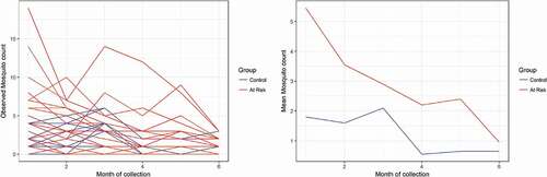
The study consists of a longitudinal count data where adult Anopheles mosquitoes resting inside human habitations were collected monthly (June 2013—November 2013) from 40 selected houses using pyrethrum spray catches (PSCs). Half of the households belong to resettled villages and are considered to be at risk of Malaria infection. The second half of the household belongs to villages located in low-risk areas (control). Figure 1 (left panel) presents the monthly female Anopheles mosquito count while the right panel presents the mean evolution over time.

Figure 1. Female Anopheles mosquito count data. Individual count (left panel) and average profile (right panel) in at risk and control villages, Jimma town, Southwest Ethiopia (June—November 2013)

2.2 The epilepsy data

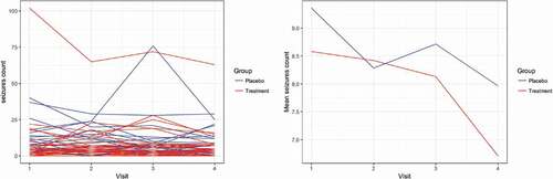
The epilepsy data set contains information about 59 epileptics’ patients that are randomized into two treatment arms, a placebo or a new drug in a randomized clinical trial of anticonvulsant therapy (Thall & Vail, 1990). The response variable, the number of epilepsy seizures, was measured at four visits over time. The data was presented and analysed by Breslow and Clayton (1993) and used as an illustrating example in Fong et al. (2010) who evaluated the performance of INLA in comparison with penalized quasi-likelihood (PQL). The epilepsy data set is available in R (R Core Team, 2016) as part of the R package INLA (Rue et al., 2009). Figure 2 shows the individual and average profiles of the epilepsy data for both treatment groups.

Figure 2. Individual profiles (left panel) and average profile (right panel) of the epilepsy data for both treatment groups

3 Hierarchical Bayesian models for count data

3.1 Hierarchical poisson-normal models

Generalized linear mixed models (GLMMs) extend the generalized linear model with a subject-specific random effect, usually of Gaussian type, added to the linear predictor to give a rich family of models that have been used in a wide variety of applications (McCulloch & Neuhaus, 2001; Molenberghs & Verbeke, 2005). The analysis presented in this paper is focused on count variables (number of female Anopheles mosquitoes and number of epilepsy seizures) which were repeatedly measured over time. Hence, we formulated a hierarchical Poisson model for both case studies. Let $Y_{ij}$ represent the response variable of the $i$th subject measured at time $j$, $i=1,2,\dots ,I$ and $j=1,2,\dots ,J$. A Poisson-Normal hierarchical (HPN) model can be formulated as

$Y_{ij}\sim Poisson({\lambda }_{ij}),$

${\eta }_{ij}=log({\lambda }_{ij})=x_{ij}^T\mathit{\beta }+b_{0i},$

(1) $b_{0i}\sim N(0,{\sigma }_{b_0}^2),$(1)

where $x_{ij}$ is a $p$-dimensional design matrix of the fixed effect parameters $\beta$ and $b_{0i}$ is a random intercept typically used to model repeated count responses. To complete the specification, we used non-informative prior distributions, namely, a normal distribution with mean zero and variance 10,000 for $\beta$‘s and considered various non-informative prior distributions for ${\sigma }_{b_0}^2$ (see Section 3.2).

The HPN model specified in (1) assumes that all sources of variability in the data can be captured by the random effects and the Poisson variability. A commonly encountered problem related to count data is overdispersion (or underdispersion), which may cause serious flaws in precision estimation and inference (Breslow, 1990) if not appropriately accounted for. A number of extensions of the HPN models have been proposed to account for extra-dispersion in the setting of longitudinal count data (2015; Aregay et al., 2013; Molenberghs et al., 2007). Aregay et al. (2015) extend the HPN model in (1) by considering two separate random effects added to the linear predictor. The mean structure for their model (HPNOD) is given by

${\eta }_{ij}=log({\lambda }_{ij})=x_{ij}^T\beta +b_{0i}+u_{ij},$

(2) $u_{ij}\sim N(0,{\sigma }_u^2),$(2)

where $b_{0i}$ is the random intercept used to account for possible clustering effect as before and the random effect $u_{ij}$ included to accommodate the overdispersion not captured by the normal random effect $b_{0i}$. The assumed priors for ${\sigma }_u^2$ are discussed in section 3.2. We choose the additive overdispersion model above rather than the multiplicative overdispersion model (Aregay et al., 2013; Molenberghs et al., 2007) to keep parametrization of the model to be the same across softwares. Further, a comparison of the additive model and the multiplicative model has been described by Aregay et al. (2015) and they reported the performance of the two approaches to be the same.

3.1.1 Model formulation for Anopheles mosquitoes count data

Let $Y_{ij}$ represent the number of female Anopheles mosquito counts for household $i$ during month $j$ of the follow-up period, let $t_{ij}$ be the time point (months) at which $Y_{ij}$ has been measured, $t_{ij}=1,\dots ,6$ for all households, and let $x_i$ be an indicator variable, which denotes the village type of the $i$th household, which takes the value of one if the household is located in a resettled (risk) village and zero if the household is located in a control village. We assumed $Y_{ij}|\beta ,b_{0i}\sim Poisson({\lambda }_{ij}),i=1,\dots ,40,j=1,\dots ,6$, and that the pattern of Anopheles mosquito abundance over time is log-linear and possibly different between the control and at-risk villages. Thus, the HPN model has a linear predictor of the form

(3) ${\eta }_{ij}=log({\lambda }_{ij})={\beta }_{00}{x}_i+{\beta }_{01}(1-x_i)+{\beta }_{10}{x}_i{t}_{ij}+{\beta }_{11}(1-x_i)t_{ij}+b_{0i},$(3)

and the mean structure for the HPNOD is given by

(4) ${\eta }_{ij}=log({\lambda }_{ij})={\beta }_{00}{x}_i+{\beta }_{01}(1-x_i)+{\beta }_{10}{x}_i{t}_{ij}+{\beta }_{11}(1-x_i)t_{ij}+b_{0i}+u_{ij}.$(4)

3.1.2 Model formulation for epilepsy data

Breslow and Clayton (1993) analyzed the epilepsy data set presented in Section 2.2 using likelihood-based inference via penalized quasi-likelihood (PQL). Fong et al. (2010) used this data set to illustrate how Bayesian inference may be performed using INLA. We concentrate on the two random-effects models fit by Breslow and Clayton (1993) and Fong et al. (2010). Let $Y_{ij}$ be the number of seizures for patient $i$ at visit $j$, $i=1,2,\dots ,59$ and $j=1,2,\dots ,4$, assumed to be conditionally independent Poisson variables with mean $exp({\lambda }_{ij})$, where the linear predictor for the HPN model is given by

${\eta }_{ij}=log({\lambda }_{ij})={\beta }_0+{\beta }_{1}log(\mathrm{B}\mathrm{a}\mathrm{s}\mathrm{e}\mathrm{l}\mathrm{i}\mathrm{n}{\mathrm{e}}_i/4)+{\beta }_2\mathrm{T}\mathrm{r}{\mathrm{t}}_i+{\beta }_3\mathrm{T}\mathrm{r}{\mathrm{t}}_i\times log(\mathrm{B}\mathrm{a}\mathrm{s}\mathrm{e}\mathrm{l}\mathrm{i}\mathrm{n}{\mathrm{e}}_i/4)$

(5) $+{\beta }_{4}log(\mathrm{A}\mathrm{g}{\mathrm{e}}_i)+{\beta }_5{V}_{4i}+b_{0i},$(5)

and the linear predictor for the HPNOD model is given by

${\eta }_{ij}=log({\lambda }_{ij}={\beta }_0+{\beta }_{1}log(\mathrm{B}\mathrm{a}\mathrm{s}\mathrm{e}\mathrm{l}\mathrm{i}\mathrm{n}{\mathrm{e}}_i/4)+{\beta }_2\mathrm{T}\mathrm{r}{\mathrm{t}}_i+{\beta }_3\mathrm{T}\mathrm{r}{\mathrm{t}}_i\times log(\mathrm{B}\mathrm{a}\mathrm{s}\mathrm{e}\mathrm{l}\mathrm{i}\mathrm{n}{\mathrm{e}}_i/4)$

(6) $+{\beta }_{4}log(\mathrm{A}\mathrm{g}{\mathrm{e}}_i)+{\beta }_5{V}_{4i}+b_{0i}+u_{ij}.$(6)

Here, $\mathrm{B}\mathrm{a}\mathrm{s}\mathrm{e}\mathrm{l}\mathrm{i}\mathrm{n}{\mathrm{e}}_i/4$ denote the one-fourth of the baseline seizure count for the $i$th patient, $\mathrm{T}\mathrm{r}{\mathrm{t}}_i$ is an indicator variable for the treatment arm of the $i$th patient, which takes the value of one if the patient is assigned to the new drug and zero if the patient is assigned to the placebo group, and $V_{4i}$ is an indicator variable for the fourth visit. To aid convergence when fitting the HPN and HPNOD models (5) and (6), respectively, the covariates $log(\mathrm{B}\mathrm{a}\mathrm{s}\mathrm{e}\mathrm{l}\mathrm{i}\mathrm{n}{\mathrm{e}}_i/4)$, $log(\mathrm{A}\mathrm{g}{\mathrm{e}}_i)$, and $\mathrm{T}\mathrm{r}{\mathrm{t}}_i\times log(\mathrm{B}\mathrm{a}\mathrm{s}\mathrm{e}\mathrm{l}\mathrm{i}\mathrm{n}{\mathrm{e}}_i/4)$ were centred about their mean.

3.2 Priors for the variance components of the hierarchical Poisson models

A Bayesian approach is attractive for modelling complex longitudinal count data, but requires the specification of prior distributions for all the random elements of the model. For the hierarchical models in Section 3.1, this involves choosing priors for the regression coefficients and the hyperparameters ${\sigma }_{b_0}^2$ and ${\sigma }_u^2$ of subject and observation-specific random effects, respectively. Two classes of prior distributions, informative and non-informative priors, are used in Bayesian modelling. One can use informative priors when substantial prior information is available, for instance, from previous studies relevant to the current data set. Non-informative prior distributions are intended to allow Bayesian inference for parameters about which little is known beyond the data included in the analysis at hand (Gelman, 2006). In this paper, we focus on the choose of non-informative prior.

The specification of a non-informative prior to express the absence of prior information about the cluster variance and overdispersion is often difficult (Gelman, 2006). Various non-informative prior distributions have been suggested in the Bayesian literature, including an improper uniform density on the scale of standard deviation (Gelman et al., 2003), proper distributions such as the $inverse-gamma(\in ,\in )$ with small positive $\in$ for the variance (Lunn et al., 2012), and conditionally conjugate folded-non-central-t family of prior distributions for the standard deviation (Gelman, 2006). In this paper, we concentrate on the latter two approaches. We considered three specifications based on $inverse-gamma(\in ,\in )$ for the variance and half-Cauchy prior (a special case of the conditionally conjugate folded-non-central-t family of prior distributions) for the standard deviation (see Figure 1 in the supplementary material):

1. $p({\sigma }^{-2})\sim \mathrm{\Gamma }(1,0.0005)$—the default choice of the INLA software (Rue et al., 2009);

2. $p({\sigma }^{-2})\sim \mathrm{\Gamma }(0.001,0.001)$—the default choice of the BUGS software (Lunn et al., 2012) and the most popular choice in Bayesian analysis;

3. $p({\sigma }^{-2})\sim \mathrm{\Gamma }(0.5,0.0164)$—a specification proposed by Fong et al. (2010);

4. Half—Cauchy prior with scale 25 on $\sigma$—a specification proposed by (Gelman, 2006).

4 Result

4.1 Analysis of the Anopheles mosquitoes count data

In this subsection, we present the analysis of the Anopheles mosquitoes count data introduced in Section 2.1. We considered three estimation routines (namely: Stan, JAGS, and INLA) where all of them are accessed through R software version 3.3.2 (R Core Team, 2016) to fit the HPN and HPNOD models presented in section 3.1.1 and 3.1.2. For the Bayesian inference using runjags (Denwood, 2016) we run 3 chains with 30,000 MCMC iterations per chain from which the first 10,000 iterations are considered burn-in period, while for RStan (Stan Development Team, 2016) the results are based on 4 chains with 4000 MCMC iterations per chain (with the first 2000 the burn-in period). Note that the models can be fitted in Stan using brms (Bürkner, 2017) as well. An elaborate discussion about two packages, RStan and brms, is given in Section 6 of the supplementary appendix. Model selection was made using the Deviance Information Criteria (DIC, Spiegelhalter et al., 2002) for INLA and JAGS and the widely applicable information criteria (WAIC, Vehtari et al., 2017) for Stan.

The posterior means and standard deviations for the parameters of the HPN and HPNOD models estimated using INLA, JAGS, and Stan using the four prior specifications are presented in Table 1. For all priors considered, the DIC and WAIC values of the HPNOD model are slightly higher than those of the HPN model, suggesting the latter to be a preferred model for this dataset.

Table 1. Parameter estimates of the HPN and HPNOD models for the Anopheles mosquitoes count data using INLA, JAGS and Stan

		Stan				JAGS				INLA
		HPN		HPNOD		HPN		HPNOD		HPN		HPNOD
Pprior	Param.	Est	sd	Est	sd	Est	SD	Est	SD	Est	sd	Est	sd
1	${\beta }_{00}$	1.55	0.23	1.55	0.22	1.55	0.23	1.55	0.23	1.56	0.23	1.56	0.23
	${\beta }_{01}$	0.69	0.27	0.71	0.28	0.70	0.26	0.69	0.26	0.69	0.26	0.69	0.26
	${\beta }_{10}$	−0.27	0.03	−0.27	0.03	−0.27	0.03	−0.27	0.03	−0.27	0.03	−0.27	0.03
	${\beta }_{11}$	−0.25	0.05	−0.25	0.05	−0.25	0.05	−0.25	0.05	−0.25	0.05	−0.25	0.05
	${\sigma }_{b_0}$	0.88	0.13	0.87	0.12	0.86	0.12	0.86	0.13	0.85	0.12	0.85	0.12
	${\sigma }_u$			0.00	0.00			0.03	0.02			0.03	0.02
	$DI{C}^{\ast }$	682.2		682.8		690.5		690.5		691.35		691.44
2	${\beta }_{00}$	1.55	0.24	1.55	0.23	1.55	0.23	1.56	0.23	1.55	0.23	1.55	0.23
	${\beta }_{01}$	0.67	0.27	0.68	0.27	0.68	0.27	0.69	0.27	0.68	0.27	0.68	0.27
	${\beta }_{10}$	−0.27	0.03	−0.28	0.03	−0.27	0.03	−0.28	0.03	−0.27	0.03	−0.28	0.03
	${\beta }_{11}$	−0.25	0.05	−0.25	0.05	−0.25	0.05	−0.25	0.05	−0.25	0.05	−0.25	0.05
	${\sigma }_{b_0}$	0.89	0.13	0.89	0.13	0.89	0.13	0.89	0.13	0.89	0.13	0.89	0.13
	${\sigma }_u$			0.04	0.05			0.08	0.05			0.08	0.05
	$DI{C}^{\ast }$	682.4		682.5		690.2		692.0		691.13		692.14
3	${\beta }_{00}$	1.55	0.23	1.55	0.23	1.55	0.23	1.56	0.23	1.55	0.23	1.55	0.23
	${\beta }_{01}$	0.68	0.27	0.68	0.27	0.69	0.26	0.70	0.27	0.69	0.26	0.69	0.27
	${\beta }_{10}$	−0.27	0.03	−0.28	0.03	−0.27	0.03	−0.28	0.03	−0.27	0.03	−0.28	0.04
	${\beta }_{11}$	−0.25	0.05	−0.25	0.05	−0.25	0.05	−0.25	0.05	−0.25	0.05	−0.25	0.05
	${\sigma }_{b_0}$	0.88	0.13	0.88	0.13	0.88	0.13	0.87	0.13	0.87	0.12	0.87	0.13
	${\sigma }_u$			0.05	0.05			0.14	0.05			0.13	0.04
	$DI{C}^{\ast }$	682.8		683.1		690.3		692.8		691.22		693.27
4	${\beta }_{00}$	1.54	0.24	1.55	0.24	1.55	0.23	1.57	0.24	1.56	0.23	1.56	0.23
	${\beta }_{01}$	0.68	0.27	0.68	0.28	0.68	0.26	0.69	0.27	0.69	0.26	0.69	0.26
	${\beta }_{10}$	−0.27	0.03	−0.28	0.03	−0.27	0.03	−0.28	0.04	−0.27	0.03	−0.28	0.03
	${\beta }_{11}$	−0.25	0.05	−0.25	0.05	−0.25	0.05	−0.25	0.05	−0.25	0.05	−0.25	0.05
	${\sigma }_{b_0}$	0.91	0.14	0.91	0.14	0.87	0.12	0.87	0.13	0.85	0.12	0.85	0.12
	${\sigma }_u$			0.10	0.06			0.14	0.06			0.12	0.05
	$DI{C}^{\ast }$	681.6		683.7		690.2		693.8		691.35		693.06
	$Tim{e}^{\ast \ast }$	4.28		4.74		2.88		6.06		2.49		2.56

* The WAIC (Vehtari et al., 2017) is reported rather than DIC for Stan.

** The computational time for INLA is in seconds whereas the computational time for JAGS and Stan is in minutes.

All prior distributions and all methods of estimations we examined yielded similar results for the regression coefficients. However, the results in Table 1 revealed the influence of the software used to fit the models and the prior specification on the parameter estimates corresponding to the random effect terms. The three estimation methods give similar point estimates for the variance of the random intercept under the $\mathrm{\Gamma }(0.001,0.001)$ and $\mathrm{\Gamma }(0.5,0.0164)$ priors in both the HPN and HPNOD models. On the other hand, the difference among estimation methods is noticeable under the $\mathrm{\Gamma }(1,0.0005)$ and half Cauchy prior, where the posterior mean for ${\sigma }_{b_0}^2$ obtained from Stan is about 6% larger than INLA under $\mathrm{\Gamma }(1,0.0005)$ prior and about 13% larger under the half Cauchy prior. Figure 3 shows the posterior density of the precision of the random intercept (${\sigma }_{b_0}^{-2}$) obtained from JAGS, Stan and INLA using the four prior distributions. All estimation methods lead to a similar result under $\mathrm{\Gamma }(0.001,0.001)$ and $\mathrm{\Gamma }(0.5,0.0164)$ priors, but the posterior density of INLA for ${\sigma }_{b_0}^{-2}$ deviates from that of Stan under the $\mathrm{\Gamma }(1,0.0005)$ and half Cauchy prior. For INLA, we observed differences in the point estimates of ${\sigma }_{b_0}^2$ and ${\sigma }_u^2$ across priors, where a profound variation across priors is observed in the posterior density of ${\sigma }_u^2$ (Figure 4).

Figure 3. Anopheles mosquitoes count data: Posterior density for the precision of the random intercept (${\sigma }_{b_0}^{-2}$) obtained for the HPN model

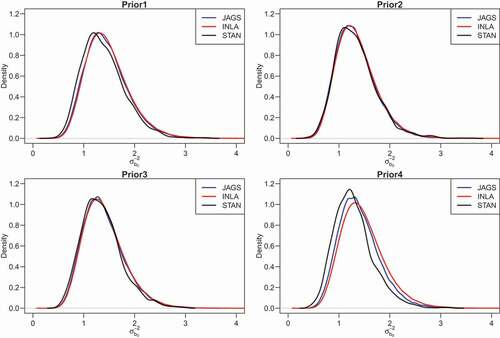
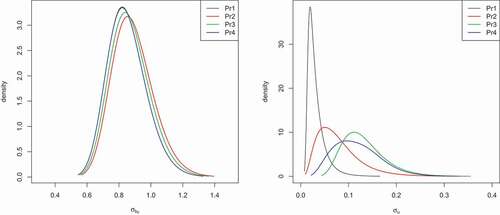
Figure 4. Anopheles mosquitoes count data: Marginal posterior distribution of ${\sigma }_b$ (left panel) and ${\sigma }_u$ (right panel) for the analysis of Anopheles mosquitoes count data using HPNOD model estimated via INLA. Pr1—$\mathrm{\Gamma }(1,0.0005)$, Pr2—$\mathrm{\Gamma }(0.001,0.001)$, Pr3—$\mathrm{\Gamma }(0.5,0.0164)$ and Pr4—(half-$Cauchy(0,25)$

4.2 Analysis of the epilepsy data

The HPN and HPNOD models formulated in equations (5)(5) $+{\beta }_{4}log(\mathrm{A}\mathrm{g}{\mathrm{e}}_i)+{\beta }_5{V}_{4i}+b_{0i},$(5) and (6(6) $+{\beta }_{4}log(\mathrm{A}\mathrm{g}{\mathrm{e}}_i)+{\beta }_5{V}_{4i}+b_{0i}+u_{ij}.$(6) ) were fitted using the three software and four priors discussed in the previous section.

Figure 5. Epilepsy data: Posterior density for the precision of the random intercept (${\sigma }_{b_0}^{-2}$) obtained for the HPNOD model

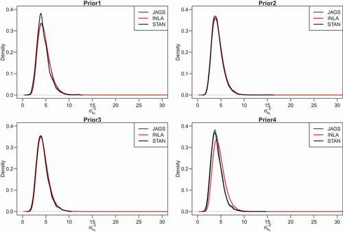
Table 2 presents the posterior means obtained for all fitted models. The DIC (WAIC) values of the HPNOD model obtained for all estimation methods are smaller than those of the HPN model for all prior settings, indicating that the first model is preferred. The three estimation methods lead to virtually identical results for the HPNOD model under priors 2 and 3. However, under the half Cauchy prior (prior 4), the posterior means for the random intercept (${\sigma }_{b_0}^2$) and overdispersion (${\sigma }_u^2$) obtained for Stan and JAGS are slightly higher than the posterior mean obtained for INLA. Figures 5 and 6 show the posterior density of the precision of the random intercept (${\sigma }_{b_0}^{-2}$) and the precision of the overdispersion parameter (${\sigma }_u^{-2}$) obtained from JAGS, Stan and INLA using the four prior distributions. We notice a small difference between JAGS and INLA as well as Stan and INLA for the two prior specifications (priors 1 and 2). Differences between estimation methods are clearly seen when the half Cauchy prior is used.

Figure 6. Epilepsy data: posterior density for the precision of the overdispersion parameter (${\sigma }_u^{-2}$) obtained for the HPNOD model

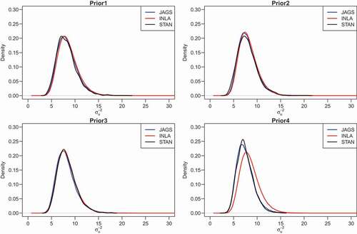
Table 2. Parameter estimates of the HPN and HPNOD models for the epilepsy data set using INLA, JAGS and stan

		Stan				JAGS				INLA
		HPN		HPNOD		HPN		HPNOD		HPN		HPNOD
PPrior	Param.	Est	sd	Est	sd	Est	SD	Est	SD	Est	sd	Est	sd
1 1	${\beta }_0$	1.62	0.08	1.57	0.08	1.62	0.08	1.58	0.07	1.62	0.08	1.58	0.08
	${\beta }_1$	0.88	0.14	0.88	0.14	0.88	0.13	0.89	0.13	0.88	0.14	0.88	0.13
	${\beta }_2$	−0.34	0.16	−0.34	0.15	−0.34	0.15	−0.33	0.15	−0.34	0.15	−0.33	0.15
	${\beta }_3$	0.34	0.21	0.35	0.21	0.34	0.20	0.35	0.20	0.34	0.21	0.35	0.21
	${\beta }_4$	0.47	0.36	0.48	0.36	0.47	0.36	0.48	0.35	0.48	0.36	0.48	0.35
	${\beta }_5$	−0.16	0.05	−0.10	0.09	−0.16	0.05	−0.10	0.09	−0.16	0.05	−0.10	0.09
	${\sigma }_{b_0}$	0.53	0.06	0.49	0.07	0.52	0.06	0.48	0.07	0.52	0.06	0.48	0.07
	${\sigma }_u$			0.36	0.04			0.35	0.04			0.35	0.04
	$DI{C}^{\ast }$	1328.4		1151.9		1271.9		1159.3		1272.3		1158.2
2 2	${\beta }_0$	1.62	0.08	1.57	0.08	1.62	0.08	1.57	0.08	1.62	0.08	1.57	0.08
	${\beta }_1$	0.88	0.14	0.88	0.14	0.88	0.15	0.88	0.14	0.88	0.14	0.88	0.14
	${\beta }_2$	−0.34	0.16	−0.33	0.16	−0.34	0.16	−0.33	0.16	−0.34	0.16	−0.33	0.16
	${\beta }_3$	0.34	0.22	0.35	0.21	0.35	0.22	0.36	0.21	0.34	0.22	0.35	0.21
	${\beta }_4$	0.47	0.37	0.48	0.37	0.47	0.38	0.48	0.37	0.47	0.37	0.48	0.36
	${\beta }_5$	−0.16	0.05	−0.10	0.09	−0.16	0.05	−0.10	0.09	−0.16	0.05	−0.10	0.09
	${\sigma }_{b_0}$	0.54	0.07	0.50	0.07	0.54	0.07	0.50	0.07	0.54	0.06	0.50	0.07
	${\sigma }_u$			0.36	0.04			0.36	0.04			0.36	0.04
	$DI{C}^{\ast }$	1328.9		1149.1		1271.75		1159.0		1272.1		1157.8
33	${\beta }_0$	1.62	0.08	1.57	0.08	1.62	0.08	1.57	0.08	1.62	0.08	1.57	0.08
	${\beta }_1$	0.88	0.14	0.88	0.14	0.88	0.13	0.89	0.14	0.88	0.14	0.88	0.14
	${\beta }_2$	−0.34	0.16	−0.33	0.15	−0.33	0.16	−0.34	0.16	−0.34	0.16	−0.33	0.15
	${\beta }_3$	0.34	0.21	0.35	0.21	0.35	0.21	0.33	0.21	0.34	0.21	0.35	0.21
	${\beta }_4$	0.48	0.37	0.49	0.36	0.49	0.37	0.46	0.36	0.48	0.37	0.48	0.36
	${\beta }_5$	−0.16	0.05	−0.10	0.09	−0.16	0.05	−0.10	0.09	−0.16	0.05	−0.10	0.09
	${\sigma }_{b_0}$	0.54	0.07	0.49	0.07	0.53	0.06	0.49	0.07	0.53	0.06	0.49	0.07
	${\sigma }_u$			0.36	0.04			0.36	0.04			0.36	0.04
	$DI{C}^{\ast }$	1326.7		1148.4		1271.5		1159.1		1272.2		1157.9
4 4	${\beta }_0$	1.62	0.08	1.57	0.08	1.62	0.08	1.57	0.08	1.62	0.08	1.58	0.08
	${\beta }_1$	0.88	0.14	0.88	0.14	0.90	0.15	0.87	0.14	0.88	0.14	0.88	0.13
	${\beta }_2$	−0.33	0.16	−0.33	0.16	−0.34	0.16	−0.33	0.16	−0.34	0.15	−0.33	0.15
	${\beta }_3$	0.34	0.22	0.35	0.22	0.31	0.22	0.36	0.22	0.34	0.21	0.35	0.21
	${\beta }_4$	0.47	0.37	0.48	0.37	0.45	0.38	0.48	0.36	0.48	0.36	0.48	0.35
	${\beta }_5$	−0.16	0.05	−0.10	0.09	−0.16	0.05	−0.10	0.09	−0.16	0.05	−0.10	0.09
	${\sigma }_{b_0}$	0.55	0.07	0.51	0.07	0.54	0.07	0.50	0.07	0.52	0.06	0.48	0.07
	${\sigma }_u$			0.37	0.04			0.37	0.04			0.35	0.04
	$DI{C}^{\ast }$	1326.5		1147.2		1271.7		1159.0		1272.3		1158.1
	$Tim{e}^{\ast \ast }$	5.80		5.44		3.23		5.06		4.30		12.78

* The WAIC (Vehtari et al., 2017) is reported rather than DIC for Stan.

** The computational time for INLA is in seconds whereas the computational time for JAGS and Stan is in minutes.

5 Simulation study

A simulation study was conducted to compare the performance of the three Bayesian software and the four prior specifications for ${\sigma }_{b_0}$ and ${\sigma }_u$ presented in Section 3.2.

5.1 Simulation setting

The simulation represents a longitudinal study where the data are Poisson distributed. The steps for the simulation study are as follows: For $i=1,\dots ,N$ clusters (subjects), $j=1,\dots ,J$ observations per cluster observed at equally spaced sampling times $t_{ij}=(t_{i1},\dots ,t_{iJ}){ }^{\mathrm{\prime }}$, we generate $Y_{ij}\sim Poisson({\lambda }_{ij})$ where

(7) ${\eta }_{ij}=log({\lambda }_{ij})={\beta }_{00}{x}_i+{\beta }_{01}(1-x_i)+{\beta }_{10}{x}_i{t}_{ij}+{\beta }_{11}(1-x_i)t_{ij}+b_{0i}+u_{ij},$(7)

with $b_{0i}\sim N(0,{\sigma }_{b_0}^2),u_{ij}\sim N(0,{\sigma }_u^2)$, and $x_i$ is an indicator variable such that $x_i=0$ for $i\le N/2$ and $x_i=1$ otherwise. The model formulated in (7) is the HPNOD model discussed in (3.1.1). Low, moderate, and high levels of overdispersion were considered corresponding to ${\sigma }_u=0.2,1$ and 2, respectively (Aregay et al., 2015). A model without overdispersion (HPN) was formulated by omitting $u_{ij}$ from the mean structure in (7). The true values of the fixed effect parameters for both the HPN and HPNOD models are $\beta =({\beta }_{00},{\beta }_{01},{\beta }_{10},{\beta }_{11}){ }^{\mathrm{\prime }}=(2,-2,0.05,0.2){ }^{\mathrm{\prime }}$. To study how the performance of the estimation methods and the role of the prior distribution are affected by the value of the cluster variance, we used four different values for the standard deviation parameter of the random intercept term, i.e ${\sigma }_{b_0}=0.1,0.5,1,1.5$. Further, in order to study the effect of small number of observations per cluster, we considered four balanced designs with $J=2,5$ observations per cluster and the number of clusters equal to $N=20$ and $40$. In total $4\times 4\times 2\times 2=64$ simulation setting was considered. For each setting 500 datasets were generated. For each dataset, the HPN and HPNOD models were fitted with INLA, JAGS, and Stan using a flat prior distribution $N(0,1000)$ for the fixed effect parameters and using the four prior distributions listed in Section 3.2 for ${\sigma }_{b_0}^2$ and ${\sigma }_u^2$. For JAGS and Stan, we ran 3 chains with 20,000 iterations per chain from which the first 10,000 iterations were considered as burn-in period. For each parameter of interest $\theta$, the relative bias was calculated by

$\frac{1}{500}{\mathrm{\Sigma }}_{i=1}^{500}\left({\hat{\theta }}_i-\theta \right)/\theta ,$

and the mean squared error (MSE) by

$\frac{1}{500}{\mathrm{\Sigma }}_{i=1}^{500}\left(Var({\hat{\theta }}_i)+{\left({\hat{\theta }}_i-\theta \right)}^2\right),$

where ${\hat{\theta }}_i$ is the parameter estimate for $\theta$ obtained for the $i$th simulation. A simulation study for unbalanced longitudinal data was conducted as well. The simulation setting and result are discussed in detail in Section 5 of the supplementary appendix.

5.2 Simulation results

5.2.1 Estimation of ${\sigma }_{b_0}$

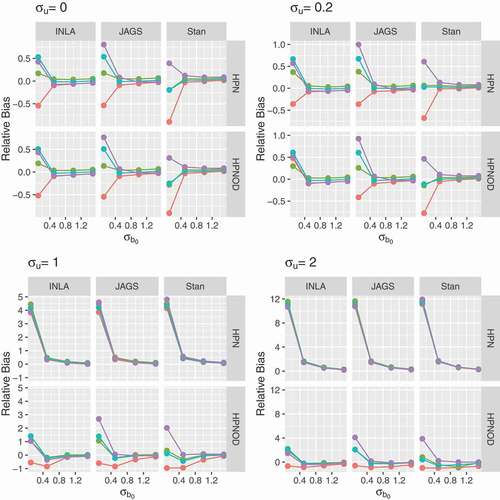
Figure 7 (upper left panel) presents the simulation results obtained for the datasets generated without overdispersion. For all prior specifications, and for all software, differences were observed for ${\sigma }_{b_0}=0.1$. For INLA and JAGS, prior 1 led to an underestimation of ${\sigma }_{b_0}$ while prior $2-4$ led to an over estimation. For Stan, prior 4 led to over estimation, while priors 1–3 led to an underestimation of ${\sigma }_{b_0}$. Note that this pattern was observed for both HPN and HPNOD, which in this case, mis-specified the mean structure (by including the over dispersion parameter).

The upper right and the lower panels in Figure 7 present the simulation results obtained for the datasets generated with varying levels of overdispersion (${\sigma }_u=0.2$, ${\sigma }_u=1$, and ${\sigma }_u=2$). In this case, the HPN model mis-specified the mean structure of the underlying model used to generate the data (by omitting the overdispersion parameter). For datasets generated with low levels of overdispersion (${\sigma }_u=0.2$), we observe a similar pattern to that of no overdispersion. When the data are generated with a moderate to high level of overdispersion, for the HPN model, all prior specifications and software have a tendency to overestimate the value of ${\sigma }_{b_0}$ with the magnitude of overestimation decreasing as the value of ${\sigma }_{b_0}$ increases. For the HPNOD model (which specified the mean structure correctly), for ${\sigma }_{b0}=0.1$, prior 1 consistently led to an under estimation of ${\sigma }_{b_0}$ across all software but with the smallest magnitude compared to the overestimation observed for the other priors.

Figure 7. Relative bias for the random intercept ${\sigma }_{b_0}$ (y-axis) as a function of the true value of ${\sigma }_{b_0}$ (x-axis); panels by level of overdispersion ${\sigma }_u$. Red lines for prior 1 ($\mathrm{\Gamma }(1,0.0005)$), green for prior 2 ($\mathrm{\Gamma }(0.001,0.001)$), light blue for prior 3 ($\mathrm{\Gamma }(0.5,0.0164)$) and purple for prior 4 (half-$Cauchy(0,25)$). $N=20$ and $J=5$

Similar patterns were observed for the second simulation study of unbalanced longitudinal data (see Section 5 of the supplementary material). When the true values for ${\sigma }_b$ are small, substantial variation is observed among software and prior specifications and this variation vanishes when the true values are relatively large.

5.2.2 Estimation of ${\sigma }_u$

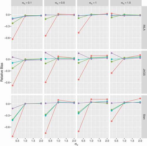
Figure 8 shows the results for the estimation of ${\sigma }_u$ across the levels of ${\sigma }_{b_0}$ for the HPNOD model. Differences between the priors can be observed for ${\sigma }_u=0.2$. For INLA and Stan, all priors led to an underestimation of ${\sigma }_u$ (prior 1 with the highest magnitude). For JAGS, prior 4 led to an overestimation of ${\sigma }_u$ while the other priors to an underestimation.

Figure 8. Relative bias for the overdispersion parameter ${\sigma }_u$ (y-axis) as a function of the true value for ${\sigma }_u$ (x-axis). Red lines for prior 1 ($\mathrm{\Gamma }(1,0.0005)$), green for prior 2 ($\mathrm{\Gamma }(0.001,0.001)$), light blue for prior 3 ($\mathrm{\Gamma }(0.5,0.0164)$) and purple for prior 4 (half-$Cauchy(0,25)$). $N=20$ and $J=5$

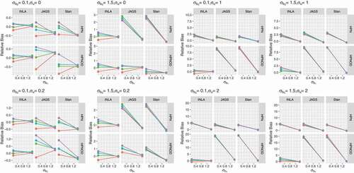
5.2.3 Estimation of $\beta$‘s

The relative biases for the regression coefficients for given values of ${\sigma }_{b_0}$ and ${\sigma }_u$ are shown in Figure 9. For INLA and Stan, all priors lead to similar relative bias for all regression coefficients under all settings. For JAGS, we observed a different pattern for ${\beta }_{10}$ when the data are generated with a high level of overdispersion (${\sigma }_u=2$) and the HPNOD model used to fit the data. The relative bias for this parameter increases in a linear fashion with the value of the standard deviation of the random intercept.

Figure 9. Relative bias for regression coefficients: ${\beta }_{00}$ (top left panel), ${\beta }_{01}$ (top right panel), ${\beta }_{10}$ (bottom left panel), and ${\beta }_{11}$ (bottom right panel). Red lines for prior 1 ($\mathrm{\Gamma }(1,0.0005)$), green for prior 2 ($\mathrm{\Gamma }(0.001,0.001)$), light blue for prior 3 ($\mathrm{\Gamma }(0.5,0.0164)$) and purple for prior 4 (half-$Cauchy(0,25)$). $N=20$ and $J=5$

5.2.4 Effect of cluster size

A simulation study also investigated the effect of a small number of observations per cluster on the estimation. Two and five observations per cluster were considered. Figure 10, presents the relative bias for all the parameters of the HPNOD model. The results obtained for $N=20$, ${\sigma }_{b_0}=1$, and ${\sigma }_u=1$ indicate that, as expected, the relative bias decreases as the sample size increases. Note that this pattern was observed for all software and priors considered. The results obtained for the HPN model are similar and presented in Section 3 of the supplementary appendix.

Figure 10. Relative bias for HPNOD model parameters (y-axis) as a function number of observation per cluster $J$ (x-axis). Red lines for prior 1 ($\mathrm{\Gamma }(1,0.0005)$), green for prior 2 ($\mathrm{\Gamma }(0.001,0.001)$), light blue for prior 3 ($\mathrm{\Gamma }(0.5,0.0164)$) and purple for prior 4 (half-$Cauchy(0,25)$). $N=20$, ${\sigma }_{b_0}=1$, and ${\sigma }_u=1$

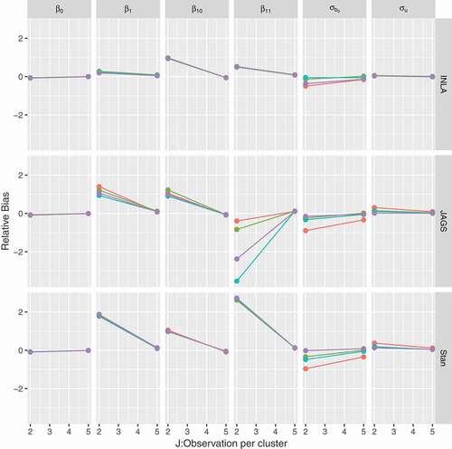
5.3 Random intercept and slope model

We extend the simulation setting in Section 5.1 to a random intercept and slope model. For $i=1,\dots ,N$ clusters (subjects), $j=1,\dots ,J$ observations per cluster observed at equally spaced sampling times $t_{ij}=(t_{i1},\dots ,t_{iJ}){ }^{\mathrm{\prime }}$, we generate $Y_{ij}\sim Poisson({\lambda }_{ij})$ where

(8) ${\eta }_{ij}=log({\lambda }_{ij})={\beta }_{00}{x}_i+{\beta }_{01}(1-x_i)+{\beta }_{10}{x}_i{t}_{ij}+{\beta }_{11}(1-x_i)t_{ij}+b_{0i}+b_{1i}{t}_{ij}+u_{ij},$(8)

with $b_{0i}\sim N(0,{\sigma }_{b_0}^2)$, $b_{1i}\sim N(0,{\sigma }_{b_1}^2)$, $u_{ij}\sim N(0,{\sigma }_u^2)$, and $x_i$ is an indicator variable such that $x_i=0$ for $i\le N/2$ and $x_i=1$ otherwise. We considered four set of values for ${\sigma }_{b_0}$ and ${\sigma }_{b_1}$, i.e $\left(\begin{array}{cc}{\sigma }_{b_0}& 0\\ 0& {\sigma }_{b_1}\end{array}\right)=\left(\begin{array}{cc}0.1& 0\\ 0& 0.1\end{array}\right),$ $\left(\begin{array}{cc}0.1& 0\\ 0& 1.5\end{array}\right),\left(\begin{array}{cc}1.5& 0\\ 0& 0.1\end{array}\right),\mathrm{a}\mathrm{n}\mathrm{d}\left(\begin{array}{cc}1.5& 0\\ 0& 1.5\end{array}\right)$. Further, low, moderate, and high levels of overdispersion were considered corresponding to ${\sigma }_u=0.2,1$ and $2$, respectively. A model without overdispersion (HPN) was formulated by omitting $u_{ij}$ from the mean structure in (8). The true values of the fixed effect parameters are $\beta =({\beta }_{00},{\beta }_{01},{\beta }_{10},{\beta }_{11}){ }^{\mathrm{\prime }}=(2,-2,0.05,0.2){ }^{\mathrm{\prime }}$. For each setting, we made 100 simulated data sets consisting of 20 subjects with 5 measurements per subject and fit the HPN and HPNOD models with INLA, JAGS, and Stan using the four prior distributions listed in Section 3.2 for ${\sigma }_{b_0}^2$, ${\sigma }_{b_1}^2$ and ${\sigma }_u^2$. For JAGS and Stan, we run 3 chains with 20,000 iterations per chain from which the first 10,000 iterations were considered as burn-in period. Then, we computed the relative bias and mean squared for each parameter (see Section 5.1).

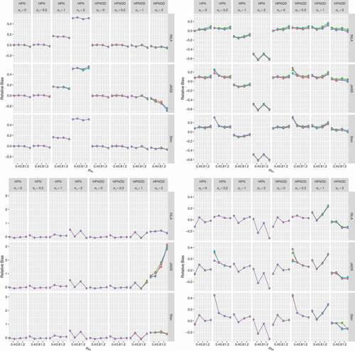
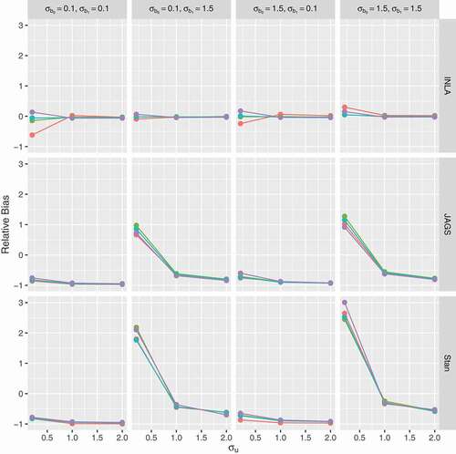
5.3.1 Estimation of ${\sigma }_{b_0}$ and ${\sigma }_{b_1}$

The relative bias for ${\sigma }_{b_0}$ obtained for the datasets generated with varying level of overdispersion (${\sigma }_u^2=0,0.2,1,\mathrm{a}\mathrm{n}\mathrm{d}2$) and different values of ${\sigma }_{b_1}$ (${\sigma }_{b_1}=0.1\mathrm{a}\mathrm{n}\mathrm{d}{\sigma }_{b_1}=1.5$) are presented in Figure 11. We observe substantial variation among priors and software when ${\sigma }_{b_0}=0.1$. When ${\sigma }_{b_0}=0.1$ and the data generated without overdispersion, Prior 1 ($\mathrm{\Gamma }(1,0.0005)$) leads to underestimation while prior 2–4 leads to overestimation for all software. The relative bias decreases as the true value for ${\sigma }_{b_0}$ increases. We also observed the influence of the level of variation in the random slope (${\sigma }_{b_1}$) on the estimate of ${\sigma }_{b_0}$ especially for JAGS.

Figure 11. Relative bias for ${\sigma }_{b_0}$ as a function of the it’s true value (x-axis); panels by level of overdispersion (${\sigma }_u$) and true values of ${\sigma }_{b_1}$. Red lines for prior 1 ($\mathrm{\Gamma }(1,0.0005)$), green for prior 2 ($\mathrm{\Gamma }(0.001,0.001)$), light blue for prior 3 ($\mathrm{\Gamma }(0.5,0.0164)$) and purple for prior 4 (half-$Cauchy(0,25)$). $N=20$ and $J=5$

Figure 12 presents the relative bias for ${\sigma }_{b_1}$ obtained for the datasets generated with varying levels of overdispersion (${\sigma }_u^2=0,0.2,1,\mathrm{a}\mathrm{n}\mathrm{d}2$) and different values of ${\sigma }_{b_0}$ (${\sigma }_{b_0}=0.1\mathrm{a}\mathrm{n}\mathrm{d}{\sigma }_{b_0}=1.5$). As before, variation among priors and software is observed when the true value for ${\sigma }_{b_1}$ is small (${\sigma }_{b_1}=0.1$) and the true value for ${\sigma }_{b_0}$ is large (${\sigma }_{b_1}=1.5$). Overall, INLA performs better than JAGS and Stan under all scenarios.

Figure 12. Relative bias for ${\sigma }_{b_1}$ as a function of the it’s true value (x-axis); panels by level of overdispersion (${\sigma }_u$) and true values of ${\sigma }_{b_0}$. Red lines for prior 1 ($\mathrm{\Gamma }(1,0.0005)$), green for prior 2 ($\mathrm{\Gamma }(0.001,0.001)$), light blue for prior 3 ($\mathrm{\Gamma }(0.5,0.0164)$) and purple for prior 4 (half-$Cauchy(0,25)$). $N=20$ and $J=5$

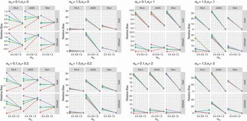
5.3.2 Estimation of ${\sigma }_u$

Figure 13 presents the relative bias for ${\sigma }_u$ obtained for the datasets generated with varying levels of overdispersion. The variation among priors decreases as the true value of overdispersion (${\sigma }_u$) increases. However, a substantial difference is observed among software. INLA performs better than JAGS and Stan under all scenarios. JAGS and Stan consistently underestimate ${\sigma }_u$ when $\left(\begin{array}{cc}{\sigma }_{b_0}& 0\\ 0& {\sigma }_{b_1}\end{array}\right)=\left(\begin{array}{cc}0.1& 0\\ 0& 0.1\end{array}\right)$ and $\left(\begin{array}{cc}0.1& 0\\ 0& 1.5\end{array}\right)$. Further, when the data are generated with $\left(\begin{array}{cc}{\sigma }_{b_0}& 0\\ 0& {\sigma }_{b_1}\end{array}\right)=\left(\begin{array}{cc}0.1& 0\\ 0& 1.5\end{array}\right)$ or $\left(\begin{array}{cc}1.5& 0\\ 0& 1.5\end{array}\right)$, JAGS and Stan overestimate ${\sigma }_u$ when ${\sigma }_u=0.2$ and underestimate ${\sigma }_u$ when ${\sigma }_u=1\mathrm{o}\mathrm{r}{\sigma }_u=2$.

Figure 13. Relative bias for ${\sigma }_u$ as a function of it’s true value (x-axis) obtained. Red lines for prior 1 ($\mathrm{\Gamma }(1,0.0005)$), green for prior 2 ($\mathrm{\Gamma }(0.001,0.001)$), light blue for prior 3 ($\mathrm{\Gamma }(0.5,0.0164)$) and purple for prior 4 (half-$Cauchy(0,25)$). $N=20$ and $J=5$

6 Concluding remarks

In this paper, we performed a Monte Carlo simulation study in order to simultaneously evaluate the performance of the Bayesian estimation methods and prior specifications for variance components in the context of longitudinal count data. We compared the results obtained with INLA to the results obtained with JAGS which uses Gibbs sampling and Stan which uses Hamiltonian Monte Carlo while assuming a variety of prior specifications for variance components. We analysed the influence of different factors such as small number of observations per cluster, different values of the random effect variance and estimation from a misspecified model on the bias and mean squared errors of the parameter estimates.

A simulation study has shown that the approximation strategy employed by INLA is accurate in general and all software leads to similar results for most of the cases considered. Estimation of the variance components, however, is difficult when their true value is small for all estimation methods and prior specifications. The estimates obtained for all software tend to be biased downward or upward depending on the prior. The results of the simulation study also show that there is an effect of cluster size. For all software and prior specifications, the relative bias for all parameters decrease as cluster size increases. For the random intercept and slope model, INLA performs better than JAGS and Stan under all scenarios. In our simulation study of the random intercept and slope model, we only considered independent prior for the random intercept and slope. Future research should focus on the comparison of different software assuming general priors for variance-covariance.

Acknowledgements

The authors gratefully acknowledge the support from VLIR-UOS. For the simulations, the Flemish Supercomputer Centre, funded by the Hercules Foundation and the Flemish Government of Belgium – department EWI, was used.

Disclosure statement

No potential conflict of interest was reported by the authors.

Supplemental data

Supplemental data for this article can be accessed here.

Additional information

Funding

The authors received no direct funding for this research.

Notes on contributors

Belay Birlie Yimer

Belay Birlie Yimer is currently a research associate at Versus Arthritis Centre for Epidemiology, Division of Musculoskeletal and Dermatological Sciences, The University of Manchester, UK. Prior to joining the University of Manchester, Belay was an assistant professor in the Department of Statistics, Jimma University, Ethiopia. He has completed his B.Sc. and M.Sc. in statistics and is currently pursuing his PhD in statistics. His main research area focuses on Bayesian methods and modelling complex time-to-event data with applications to infectious and chronic diseases.

Ziv Shkedy

Ziv Shkedy is a Professor of Biostatistics and bioinformatics at the University of Hasselt in Belgium.

References

- Aregay, M., Shkedy, Z., & Molenberghs, G. (2013). A hierarchical bayesian approach for the analysis of longitudinal count data with overdispersion: A simulation study. Computational Statistics & Data Analysis, 57(1), 233–16. https://doi.org/https://doi.org/10.1016/j.csda.2012.06.020
- Aregay, M., Shkedy, Z., & Molenberghs, G. (2015). Comparison of additive and multiplicative bayesian models for longitudinal count data with overdispersion parameters: A simulation study. Communications in Statistics-Simulation and Computation, 44(2), 454–473. https://doi.org/https://doi.org/10.1080/03610918.2013.781629
- Breslow, N. (1990). Tests of hypotheses in overdispersed poisson regression and other quasilikelihood models. Journal of the American Statistical Association, 85(410), 565–571. https://doi.org/https://doi.org/10.1080/01621459.1990.10476236
- Breslow, N. E., & Clayton, D. G. (1993). Approximate inference in generalized linear mixed models. Journal of the American Statistical Association, 88(421), 9–25. https://www.jstor.org/stable/2290687
- Bürkner, P. (2017). brms: An R Package for Bayesian Multilevel Models Using Stan. Journal of Statistical Software, 80(1), 1-28. https://doi.org/http://doi.org/10.18637/jss.v080.i01
- Core Team, R. (2016). R: A language and environment for statistical computing. R Foundation for Statistical Computing. URL https://www.R-project.org/
- Degefa, T., Zeynudin, A., Godesso, A., Michael, Y. H., Eba, K., Zemene, E., Emana, D., Birlie, B., Tushune, K., & Yewhalaw, D. (2015). Malaria incidence and assessment of entomological indices among resettled communities in Ethiopia: A longitudinal study. Malaria Journal, 14(1), 24. https://doi.org/https://doi.org/10.1186/s12936-014-0532-z
- Denwood, M. J. (2016). runjags: An R package providing interface utilities, model templates, parallel computing methods and additional distributions for MCMC models in JAGS. Journal of Statistical Software, 71(9), 1–25. https://doi.org/https://doi.org/10.18637/jss.v071.i09
- Ferkingstad, E., Rue, H., et al. (2015). Improving the INLA approach for approximate bayesian inference for latent gaussian models. Electronic Journal of Statistics, 9(2), 2706–2731. https://doi.org/https://doi.org/10.1214/15-EJS1092
- Fong, Y., Rue, H., & Wakefield, J. (2010). Bayesian inference for generalized linear mixed models. Biostatistics, 11(3), 397–412. https://doi.org/https://doi.org/10.1093/biostatistics/kxp053
- Gelman, A. (2006). Prior distributions for variance parameters in hierarchical models (comment on article by browne and draper). Bayesian Analysis, 1(3), 515–534. https://doi.org/https://doi.org/10.1214/06-BA117A
- Gelman, A., Carlin, J. B., Stern, H. S., & Rubin, D. B., 2003. Bayesian data analysis, (chapman & hall/crc texts in statistical science).
- Grilli, L., Metelli, S., & Rampichini, C. (2015). Bayesian estimation with integrated nested Laplace approximation for binary logit mixed models. Journal of Statistical Computation and Simulation, 85(13), 2718–2726. https://doi.org/https://doi.org/10.1080/00949655.2014.935377
- Lunn, D., Jackson, C., Best, N., Thomas, A., & Spiegelhalter, D. (2012). The BUGS book: A practical introduction to Bayesian analysis. CRC press.
- McCulloch, C. E., & Neuhaus, J. M. (2001). Generalized linear mixed models. Wiley Online Library.
- Molenberghs, G., & Verbeke, G. (2005). Missing data concepts. Models for Discrete Longitudinal Data, 481–488.
- Molenberghs, G., Verbeke, G., & Demétrio, C. G. (2007). An extended random-effects approach to modeling repeated overdispersed count data. . Lifetime Data Analysis, 13(4), 513–531. https://doi.org/https://doi.org/10.1007/s10985-007-9064-y
- Plummer, M., 2003. JAGS: A program for analysis of bayesian graphical models using Gibbs sampling. In: Proceedings of the 3rd international workshop on distributed statistical computing. Vol. 124. Vienna, p. 125.
- Rue, H., Martino, S., & Chopin, N. (2009). Approximate bayesian inference for latent gaussian models by using integrated nested Laplace approximations. Journal of the Royal Statistical Society. Series B, Statistical Methodology, 71(2), 319–392. https://doi.org/https://doi.org/10.1111/j.1467-9868.2008.00700.x
- Spiegelhalter, D. J., Best, N. G., Carlin, B. P., & Van Der Linde, A. (2002). Bayesian measures of model complexity and fi. Journal of the Royal Statistical Society. Series B, Statistical Methodology, 64(4), 583–639. https://doi.org/https://doi.org/10.1111/1467-9868.00353
- Stan Development Team, 2015. Stan: A C++ library for probability and sampling, version 2.5. 0.”.
- Stan Development Team. (2016). RStan: The R interface to Stan. version, 2.12, 1.
- Taylor, B. M., & Diggle, P. J. (2013). INLA or MCMC? a tutorial and comparative evaluation for spatial prediction in log-gaussian cox processes. Journal of Statistical Computation and Simulation, 84(10), 2266-2284.
- Thall, P. F., & Vail, S. C. (1990). Some covariance models for longitudinal count data with overdispersion. Biometrics, 46(3), 657–671. https://doi.org/https://doi.org/10.2307/2532086
- Vehtari, A., Gelman, A., & Gabry, J. (2017). Practical bayesian model evaluation using leave- one-out cross-validation and waic. Statistics and Computing, 27(5), 1413–1432. https://doi.org/https://doi.org/10.1007/s11222-016-9696-4