Wolfram Mathematica application to determination of the number of solutions for certain nonlinear boundary value problems

ABSTRACT

The nonlinear boundary value problem (BVP) $x{ }^{\mathrm{\prime }}{ }^{\mathrm{\prime }}=-ax+q(t)x\phi (x)$, where $\phi (x)=x$ or $\phi (x)=x^2$, $x{ }^{\mathrm{\prime }}(-1)=x{ }^{\mathrm{\prime }}(1)=0$ with step-wise function $q(t)$, is studied. The number of nontrivial solutions for the problem is estimated. For the case, where $q(t)=b=const>0$, the exact number of solutions for the boundary value problem is given. With the help of Wolfram Mathematica, the examples show several ways to determine the number of solutions for BVP.

KEYWORDS:

• Boundary value problem
• step-wise function
• quadratic nonlinearity
• cubic nonlinearity
• phase trajectory
• multiplicity of solutions
• jacobian elliptic function

PUBLIC INTEREST STATEMENT

In the theory of nonlinear boundary value problems for ordinary differential equations the most important and the most intensively studied is the solvability problem. Very often practical problems have a set of solutions that should be investigated, classified, approximated numerically and interpreted. Even for the second order autonomous differential equations there are problems that can be described in terms of phase portraits, even integrated and nevertheless it is lacking information to satisfactory treat them. We succeeded also in providing the explicit expressions for solutions of the respective Cauchy problems. The mentioned expressions use the Jacobian elliptic functions. Adaptation of known formulas for the cases under consideration was a bit technical. The result however was satisfactory. The exact number of solutions was provided. This investigation has been used in mathematical models of practical applications.

1. Introduction

The nonlinear oscillation in physics and applied mathematics has been intensively studied in many articles. Many papers, such as (Beléndez et al., 2017), (Beléndez et al., 2010), (Beléndez et al., 2016), (Elías-Zúñiga, 2013) presented analytical approximations to the periodic solutions and, in particular, to periodic solutions for oscillators described by ordinary differential equations with the odd-degree nonlinearity.

Studying the works of many researchers, for example, (Shafiq & Khalique, 2020), (Shafiq & Hammouch, 2020),(Shafiq et al.), (Shafiq & Sindhu, 2017), which describe physical processes, we may find that the practical applicability of these works is consistent with our theoretical studies.

An alternative possibility of studying and solving differential equations is by using the method of Lie algebras. It was mentioned in (Shang, 2012), that Lie algebra solution of differential equations has found host of useful applications in physical systems, where wealthy symmetries exist. “In many physical or chemical systems, biological or epidemic models often lack of symmetries, which adds difficulty in finding a proper Lie algebra.” An example (SIS epidemic spreading) of the application of this method was analysed in (Shang, 2012). This remark can be an impetus for the application of this method in the study of problems similar to those investigated in our article.

Motivated by these papers, the author in the current work wishes to find the exact formula for solutions (of the above-described equations) using Jacobian elliptic functions. Previous results of the author in this direction were published in a series of papers (Kirichuka, 2020), (Kirichuka, 2019), (Kirichuka & Sadyrbaev, 2018a), (Kirichuka and Sadyrbaev, Kirichuka & Sadyrbaev, 2018b).

The novelty of this research is that three ways to estimate the number of solutions to the boundary value problem are brought together.

However, insufficient attention has been paid to differential equation with even-degree nonlinearities. Although, for example, the quadratic nonlinearity has a practical application. As written in the work (Kovacic, 2020), this equation “has been used as a mathematical model of human eardrum oscillations”. This fact motivated the search for an exact solution of differential equation with quadratic nonlinearity. Equations with quadratic nonlinearities were studied in (Chicone, 1987).

Solution methodology consists of three types (ways) of obtaining an estimate of the number of solutions. One of the ways that is widely used to estimate the number of solutions is the phase plane method, when we analyze the phase portrait of the equation and the monotonicity properties of solutions. The second way to determine the number of solutions is to analyze the exact graph of a solution function or graphs of systems solutions. The third method is to study the behavior of curves consisting of endpoints of trajectories on a given interval.

In this article, we study the nonlinear boundary value problem

(1) $x{ }^{\mathrm{\prime }}{ }^{\mathrm{\prime }}=-ax+q(t)x\phi (x),a>0,$(1)

(2) $x{ }^{\mathrm{\prime }}(-1)=0x{ }^{\mathrm{\prime }}(1)=0,$(2)

where $q(t)$ is a step-wise function

(3) $q(t)=\left\{\begin{array}{c}b,t\in [-1,-1+\delta ]=:I_1,\\ 0,t\in (-1+\delta ,1-\delta )=:I_2,\\ b,t\in [1-\delta ,1]=:I_3,b>0,0<\delta <1.\end{array}\right.$(3)

We consider two cases of function $\phi (x)$: $\phi (x)=x$ or $\phi (x)=x^2$. In the first case, the equation is quadratic in the side subintervals and linear in the middle subinterval, in the second case the equation is cubic in the side subintervals and linear one in the middle subinterval.

In our problem, we are dealing with three parameters $a$, $b$ and $\delta$ and their influence on the number of solutions. There are multiple articles devoted to the study of differential equations, combined of several ones on disjoint subintervals of the main interval, for example, (Gritsans & Sadyrbaev, 2015), (Ellero & Zanolin, 2013), (Kirichuka and Sadyrbaev, 2018), (Kirichuka, 2016), (Moore & Nehari, 1959). In the paper (Kirichuka & Sadyrbaev, 2018a) an equation with cubic nonlinearity and step-wise potentials were studied together with the Dirichlet conditions.

We would like to study the same problems and compare the number of solutions. The differential equation (1) is a nonlinear equation with the quadratic or cubic nonlinearity that is switched off in a middle subinterval. We consider corresponding equations

(4) $x{ }^{\mathrm{\prime }}{ }^{\mathrm{\prime }}=-ax+b{x}^2$(4)

and

(5) $x{ }^{\mathrm{\prime }}{ }^{\mathrm{\prime }}=-ax+b{x}^3,$(5)

that contain only the quadratic or cubic nonlinearity. The Equation (1)(1) $x{ }^{\mathrm{\prime }}{ }^{\mathrm{\prime }}=-ax+q(t)x\phi (x),a>0,$(1) contains Equation (4)(4) $x{ }^{\mathrm{\prime }}{ }^{\mathrm{\prime }}=-ax+b{x}^2$(4) and (5) that were studied previously in (Kirichuka & Sadyrbaev, 2019), (Kirichuka, 2018), (Kirichuka, 2017), (Kirichuka, 2013), (Ogorodnikova & Sadyrbaev, 2006) and are included often in textbooks. We are not aware however of precise estimation of the number of solutions for the two-point BVP (1), (2). We study the problem (1), (2), where Equation (1)(1) $x{ }^{\mathrm{\prime }}{ }^{\mathrm{\prime }}=-ax+q(t)x\phi (x),a>0,$(1) is a differential equation of the type (4) or (5) in two side subintervals $I_1$ and $I_3$ and is linear in the middle subinterval $I_2$. The solutions in two side subintervals are described in terms of Jacobian elliptic functions (Gradshteyn & Ryzhik, 2000), (Milne-Thomson, 1972), (Whittaker & Watson, 1940, 1996). In the middle subinterval equation is linear $x{ }^{\mathrm{\prime }}{ }^{\mathrm{\prime }}=-ax$. The problem is to smoothly connect solutions in all subintervals. We compose a non-differential system of equations that gives the initial values of solutions for BVP (1), (2).

Our results are:

• the estimates of the number of solutions for the BVP (4), (2) and (5), (2) and their dependence on coefficient $a$;

• the systems that produce solutions of the BVP (1), (2) are given for both choices of the function $\phi (x)$: $\phi (x)=x$ or $\phi (x)=x^2$;

• the estimates of the number of solutions for the BVP (1), (2) are obtained;

• the examples are analyzed that show the validity of the above mentioned results and illustrate them.

The structure of the paper is the following. In the next section (Section 2) we describe previously obtained results on the Neumann problem for the quadratic and cubic equations. In Section 3 we obtain the systems that produce solutions of the BVP (1), (2) for both choices of the function $\phi (x)$: $\phi (x)=x$ or $\phi (x)=x^2$. The equations in those systems are obtained using the theory of Jacobian elliptic functions ((Gradshteyn & Ryzhik, 2000), (Milne-Thomson, 1972), (Whittaker & Watson, 1940, 1996)). In Section 4 we provide the main result on the number of solutions to the problem (1), (2) and we demonstrate how all the developed technique and formulas work in a specific example. In Section 5 we discuss the results and the novelty of the work.

2. Review of results on the number of solutions for the equations with quadratic and cubic nonlinearity

For the case, where $q(t)=b=const>0$ in Equation (1)(1) $x{ }^{\mathrm{\prime }}{ }^{\mathrm{\prime }}=-ax+q(t)x\phi (x),a>0,$(1) . Consider the equation with quadratic nonlinearity that is given in (4). There are two critical points of Equation (4)(4) $x{ }^{\mathrm{\prime }}{ }^{\mathrm{\prime }}=-ax+b{x}^2$(4) at $x_1=0$ and $x_2=\frac{a}{b}$. The point $x_1=0$ is a center, but $x=\frac{a}{b}$ is a saddle as shown in Figure 1. The region bounded by homoclinic orbit is denoted G2.

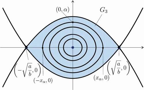
Consider the Equation (5)(5) $x{ }^{\mathrm{\prime }}{ }^{\mathrm{\prime }}=-ax+b{x}^3,$(5) , there are three critical points of equation (5) at $x_1=-\sqrt{\frac{a}{b}}$, $x_2=0$, $x_3=\sqrt{\frac{a}{b}}$. The point $x_2=0$ is a center and $x_{1,3}=\pm \sqrt{\frac{a}{b}}$ both are saddle points. Two heteroclinic trajectories connect the two saddle points. The phase portrait of Equation (5) is depicted in Figure 2. The region bounded by two heteroclinic orbits is denoted G3.

Figure 1. The phase portrait of equation $x{ }^{\mathrm{\prime }}{ }^{\mathrm{\prime }}=-ax+b{x}^2$

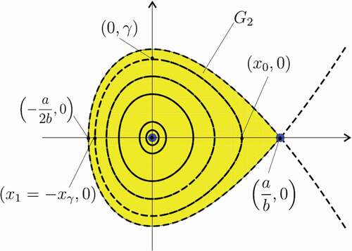
Figure 2. The phase portrait of equation $x{ }^{\mathrm{\prime }}{ }^{\mathrm{\prime }}=-ax+b{x}^3$

Consider the Cauchy problem (4),

(6) $x(-1)=x_0,x{ }^{\mathrm{\prime }}(-1)=0,0<x_0<\frac{a}{b}.$(6)

It was proved in the article (Chicone, 1988), that the period of a solution to the problem (4), (2) is increasing function of $x_0$. Therefore, the following statement is true.

Theorem 1 Let $i$ be a positive integer such that

(7) $\frac{i\pi }{2}<\sqrt{a}<\frac{(i+1)\pi }{2}.$(7)

The Neumann problem (4), (2) has exactly $2i$ nontrivial solutions such that $x(-1)=x_0$, $x{ }^{\mathrm{\prime }}(-1)=0$, $-\frac{a}{2b}<x_0<\frac{a}{b}$, $x_0\ne 0$.

The similar theorem and proof were provided in the article (Kirichuka & Sadyrbaev, 2019).

Consider the Cauchy problem (5),

(8) $x(-1)=x_{\alpha },x{ }^{\mathrm{\prime }}(-1)=0,-\sqrt{\frac{a}{b}}<x_{\alpha }<\sqrt{\frac{a}{b}},x_{\alpha }\ne 0,$(8)

Theorem 2 Let $i$ be a positive integer such that

(9) $\frac{i\pi }{2}<\sqrt{a}<\frac{(i+1)\pi }{2}.$(9)

The Neumann problem (5), (2) has exactly $2i$ nontrivial solutions such that $x(-1)=x_{\alpha }$, $x{ }^{\mathrm{\prime }}(-1)=0,$ $-\sqrt{\frac{a}{b}}<x_{\alpha }<\sqrt{\frac{a}{b}}$, $x_{\alpha }\ne 0$.

The proof of Theorem 2 can be found in the articles (Kirichuka, 2019) and (Kirichuka & Sadyrbaev, 2018a).

Proposition 1 The number of nontrivial solutions for BVP (4), (2) and (5), (2) is the same and depends on the choice of coefficient $a$.

3. Systems that produce solutions to the BVP with linear-quadratic and linear-cubic equations

3.1. BVP with linear-quadratic equations

In the formulations below the Jacobian elliptic functions $\mathrm{c}\mathrm{d},$ $\mathrm{s}\mathrm{d},$ $\mathrm{n}\mathrm{d}$ are used.

A solution of the Cauchy problem (4), $x(0)=x_0$, $x{ }^{\mathrm{\prime }}(0)=0$, $0<x_0<\frac{a}{b}$ is

(10) $\begin{array}{rl}& x(t,a,b,x_0)=x_1+(x_0-x_1)\mathrm{c}\mathrm{d}{ }^2\\ & \left(\sqrt{\frac{1}{6}b(x_2-x_1)}t,k\right),k=\sqrt{\frac{x_0-x_1}{x_2-x_1}},\\ & x_{1,2}(x_0)=\frac{1}{4b}\\ & \left(3a-2b{x}_0\mp \sqrt{3(3a-2b{x}_0)(a+2b{x}_0)}\right).\end{array}$(10)

Denoting $f(t,a,b,x_0)=x{{ }^{\mathrm{\prime }}}_t(t,a,b,x_0)$, we get

$f(t,a,b,x_0)=\sqrt{\frac{2}{3}b(x_2-x_1)}(x_0-x_2)k^2\mathrm{c}\mathrm{d}\left(\sqrt{\frac{1}{6}b(x_2-x_1)}t;k\right)\times$

(11) $\times \mathrm{n}\mathrm{d}\left(\sqrt{\frac{1}{6}b(x_2-x_1)}t;k\right)\mathrm{s}\mathrm{d}\left(\sqrt{\frac{1}{6}b(x_2-x_1)}t;k\right).$(11)

Formulas (10) and (11) were obtained in article (Kirichuka & Sadyrbaev, 2019).

Consider Equation (1), where $\phi (x)=x$ and $q(t)$ is a step-wise function given by (3). Hence, we have the problems

(12) $\begin{array}{rl}& x{ }^{\mathrm{\prime }}{{ }^{\mathrm{\prime }}}_1=-a{x}_1+b{x}_1^2,x_1(-1)=x_{\gamma },x{{ }^{\mathrm{\prime }}}_1(-1)=0,\\ & t\in I_1,0x_{\gamma }\frac{a}{b},\\ & x{ }^{\mathrm{\prime }}{{ }^{\mathrm{\prime }}}_2=-a{x}_2,x_2(-1+\delta )\\ & =x_1(-1+\delta ),x_2(1-\delta )=x_3(1-\delta ),\\ & t\in I_2,\\ & x{ }^{\mathrm{\prime }}{{ }^{\mathrm{\prime }}}_3=-a{x}_3+b{x}_3^2,x_3(1)=x_{\alpha },\\ & x{{ }^{\mathrm{\prime }}}_3(1)=0,t\in I_3,0<x_{\alpha }<\frac{a}{b}.\end{array}$(12)

Using the change of the independent variable ($t\to t-1$, $t\to t+1$) in (10), solutions of the problems

(13) $x{ }^{\mathrm{\prime }}{ }^{\mathrm{\prime }}=-ax+b{x}^2,x(-1)=x_{\gamma },x{ }^{\mathrm{\prime }}(-1)=0,$(13)

(14) $x{ }^{\mathrm{\prime }}{ }^{\mathrm{\prime }}=-ax+b{x}^3,x(1)=x_{\alpha },x{ }^{\mathrm{\prime }}(1)=0$(14)

are, respectively

(15) $\begin{array}{rl}& {\tilde{x}}_1(t,x_{\gamma })=x_1+(x_{\gamma }-x_1)\mathrm{c}{\mathrm{d}}^2\\ & \left(\sqrt{\frac{1}{6}b(x_2-x_1)}(t+1),k\right),k=\sqrt{\frac{x_{\gamma }-x_1}{x_2-x_1}},x_{1,2}(x_{\gamma })\\ & =\frac{1}{4b}\left(3a-2b{x}_{\gamma }\mp \sqrt{3(3a-2b{x}_{\gamma })(a+2b{x}_{\gamma })}\right)\\ & x_1(t,x_{\gamma })=x_1+(x_{\gamma }-x_1)\mathrm{c}{\mathrm{d}}^2\left(\sqrt{\frac{1}{6}b(x_2-x_1)}(t+1),k\right)\\ & ,k=\sqrt{\frac{x_{\gamma }-x_1}{x_2-x_1}},x_{1,2}(x_{\gamma })=\frac{1}{4b}\\ & \left(3a-2b{x}_{\gamma }\mp \sqrt{3(3a-2b{x}_{\gamma })(a+2b{x}_{\gamma })}\right)\end{array}$(15)

and

(16) $\begin{array}{rl}& {\tilde{x}}_3(t,x_{\alpha })=x_3+(x_{\alpha }-x_3)\mathrm{c}{\mathrm{d}}^2\\ & \left(\sqrt{\frac{1}{6}b(x_4-x_3)}(t-1),k_1\right),\\ & k_1=\sqrt{\frac{x_{\alpha }-x_3}{x_4-x_3}},x_{3,4}(x_{\alpha })=\frac{1}{4b}\\ & \left(3a-2b{x}_{\alpha }\mp \sqrt{3(3a-2b{x}_{\alpha })(a+2b{x}_{\alpha })}\right).\end{array}$(16)

The trajectories ${\tilde{x}}_1(t)$ and ${\tilde{x}}_3(t)$ are located in G2. In order $x(t)$ to be $C^2$-function both solutions ${\tilde{x}}_1$ and ${\tilde{x}}_3$ are to be smoothly connected by a middle function ${\tilde{x}}_2(t)$:

(17) ${\tilde{x}}_2(t)=C_{1}sin\sqrt{a}t+C_{2}cos\sqrt{a}t.$(17)

In order for the solutions ${\tilde{x}}_1(t)$, ${\tilde{x}}_3(t)$ and ${\tilde{x}}_2(t)$ to connect smoothly, it is necessary for them to satisfy the following system. The following relations are to be satisfied:

(18) $\begin{array}{rl}& {\tilde{x}}_1(-1+\delta )={\tilde{x}}_2(-1+\delta ),\\ & {\tilde{x}}_1(-1+\delta )={\tilde{x}}_2(-1+\delta ),\\ & {\tilde{x}}_3(1-\delta )={\tilde{x}}_2(1-\delta ),\\ & {\tilde{x}}_3(1-\delta )={\tilde{x}}_2(1-\delta ).\end{array}$(18)

We solve the system (18) with respect to constants $C_1$ and $C_2$. For this, we insert formulas (15), (16), (17) into the system (18). Then, making the certain transformations, we find constants $C_1$ and $C_2$, equating them and find the expressions of solutions in formulas (19), (22). We get

$\begin{array}{rl}& \mathrm{\Phi }(x_{\gamma },x_{\alpha })=sin\sqrt{a}(\delta -1)\\ & \sqrt{\frac{2}{3}b(x_4-x_3)}(x_{\alpha }-x_4)k^2\mathrm{c}\mathrm{d}\\ & \left(\sqrt{\frac{1}{6}b(x_2-x_1)}\delta ;k\right)\\ & \times \mathrm{n}\mathrm{d}\left(\sqrt{\frac{1}{6}b(x_2-x_1)}\delta ;k\right)\\ & \mathrm{s}\mathrm{d}\left(\sqrt{\frac{1}{6}b(x_2-x_1)}\delta ;k\right)\\ & -\sqrt{\frac{2}{3}b(x_4-x_3)}(x_{\alpha }-x_4)k_1^2\times \end{array}$

$\begin{array}{rl}& \times \mathrm{n}\mathrm{d}\left(\sqrt{\frac{1}{6}b(x_2-x_1)}\delta ;k\right)\\ & \mathrm{s}\mathrm{d}\left(\sqrt{\frac{1}{6}b(x_2-x_1)}\delta ;k\right)\\ & -\sqrt{\frac{2}{3}b(x_4-x_3)}(x_{\alpha }-x_4)k_1^2\times \end{array}$

$\times \text{cd}\left(\sqrt{\frac{1}{6}b(x_4-x_3)}\delta ;k_1\right)\text{nd}\left(\sqrt{\frac{1}{6}b(x_4-x_3)}\delta ;k_1\right)\text{sd}\left(\sqrt{\frac{1}{6}b(x_4-x_3)}\delta ;k_1\right)-$

$\begin{array}{rl}& -\sqrt{a}cos\sqrt{a}(\delta -1)\\ & \left[\begin{array}{c}{x}_1-x_3+(x_{\gamma }-x_1)\mathrm{c}{\mathrm{d}}^2\\ \left(\sqrt{\frac{1}{6}b(x_2-x_1)}\delta ,k\right)-(x_{\alpha }-x_3)\times \end{array}\right.\end{array}$

(19) $\left.\times \mathrm{c}\mathrm{d}{}^2\left(\sqrt{\frac{1}{6}b(x_4-x_3)}\delta ,k_1\right)\right],$(19)

$\begin{array}{rl}& \mathrm{\Psi }(x_{\gamma },x_{\alpha })=cos\sqrt{a}(\delta -1).\\ & \left[\begin{array}{c}\sqrt{\frac{2}{3}b(x_2-x_1)}(x_{\gamma }-x_2)k^2\mathrm{c}\mathrm{d}\\ \left(\sqrt{\frac{1}{6}b(x_2-x_1)}\delta ;k\right)\times \end{array}\right.\end{array}$

$\begin{array}{rl}& \times \mathrm{n}\mathrm{d}\left(\sqrt{\frac{1}{6}b(x_2-x_1)}\delta ;k\right)\\ & \mathrm{s}\mathrm{d}\left(\sqrt{\frac{1}{6}b(x_2-x_1)}\delta ;k\right)\\ & +\sqrt{\frac{2}{3}b(x_4-x_3)}(x_{\alpha }-x_4)k_1^2\times \end{array}$

$\left.\begin{array}{c}\times \mathrm{c}\mathrm{d}\left(\sqrt{\frac{1}{6}b(x_4-x_3)}\delta ;k_1\right)\\ \mathrm{n}\mathrm{d}\left(\sqrt{\frac{1}{6}b(x_4-x_3)}\delta ;k_1\right)\\ \mathrm{s}\mathrm{d}\left(\sqrt{\frac{1}{6}b(x_4-x_3)}\delta ;k_1\right)\end{array}\right]+$

$+\sqrt{a}sin\sqrt{a}(\delta -1)[x_1+x_3+(x_{\gamma }-x_1)cd{}^2\left(\sqrt{\frac{1}{6}b(x_2-x_1)}\delta ,k\right)+(x_{\alpha }-x_3)\times$

(20) $\left.\times \mathrm{c}\mathrm{d}{}^2\left(\sqrt{\frac{1}{6}b(x_4-x_3)}\delta ,k_1\right)\right].$(20)

To simplify formulas (19), (22) we denote $A=\sqrt{\frac{1}{6}b(x_2-x_1)}$ and $B=\sqrt{\frac{1}{6}b(x_4-x_3)}.$ Then we have

$\begin{array}{rl}& \mathrm{\Phi }(x_{\gamma },x_{\alpha })=sin\sqrt{a}(\delta -1)\\ & \left[\begin{array}{c}\sqrt{\frac{2}{3}b(x_2-x_1)}(x_{\gamma }-x_2)k^2\\ \mathrm{c}\mathrm{d}\left(A\delta ;k\right)\mathrm{n}\mathrm{d}\left(A\delta ;k\right)sd\left(A\delta ;k\right)-\end{array}\right.\end{array}$

$\left.\begin{array}{c}-\sqrt{\frac{2}{3}b(x_4-x_3)}(x_{\alpha }-x_4)\\ k_1^2\mathrm{c}\mathrm{d}\left(B\delta ;k_1\right)\mathrm{n}\mathrm{d}\left(B\delta ;k_1\right)\\ \mathrm{s}\mathrm{d}\left(B\delta ;k_1\right)\end{array}\right]-$

(21) $\begin{array}{rl}& -\sqrt{a}cos\sqrt{a}(\delta -1)\\ & \left[\begin{array}{c}{x}_1-x_3+(x_{\gamma }-x_1)\mathrm{c}{\mathrm{d}}^2\\ \left(A\delta ,k\right)-(x_{\alpha }-x_3)\mathrm{c}{\mathrm{d}}^2\\ \left(B\delta ,k_1\right)\end{array}\right],\end{array}$(21)

$\begin{array}{rl}& \mathrm{\Psi }(x_{\gamma },x_{\alpha })=cos\sqrt{a}(\delta -1)\\ & \left[\begin{array}{c}\sqrt{\frac{2}{3}b(x_2-x_1)}(x_{\gamma }-x_2)\\ k^2\mathrm{c}\mathrm{d}\left(A\delta ;k\right)\mathrm{n}\mathrm{d}\left(A\delta ;k\right)\\ \mathrm{s}\mathrm{d}\left(A\delta ;k\right)+\end{array}\right.\end{array}$

$\left.\begin{array}{c}+\sqrt{\frac{2}{3}b(x_4-x_3)}(x_{\alpha }-x_4)\\ k_1^2\mathrm{c}\mathrm{d}\left(B\delta ;k_1\right)\\ \mathrm{n}\mathrm{d}\left(B\delta ;k_1\right)\\ \mathrm{s}\mathrm{d}\left(B\delta ;k_1\right)\end{array}\right]+$

(22) $\begin{array}{rl}& +\sqrt{a}sin\sqrt{a}(\delta -1)\\ & \left[\begin{array}{c}{x}_1+x_3+(x_{\gamma }-x_1)\mathrm{c}{\mathrm{d}}^2\left(A\delta ,k\right)\\ +(x_{\alpha }-x_3)\mathrm{c}{\mathrm{d}}^2\left(B\delta ,k_1\right)\end{array}\right].\end{array}$(22)

The system

(23) $\left\{\begin{array}{c}\mathrm{\Phi }(x_{\gamma },x_{\alpha })=0,\\ \mathrm{\Psi }(x_{\gamma },x_{\alpha })=0\end{array}\right.$(23)

is obtained. We are interested in the number of solutions of boundary value problem (1), (2), where in (1) $\phi (x)=x$.

Proposition 2 For $a$, $b$ and $\delta$ given a nontrivial solution $(x_{\gamma },x_{\alpha })$ of the system (23) produces a solution of the Neumann problem (1),(2), where in (1) $\phi (x)=x$.

3.2. BVP with linear-cubic equations

The solution of the Cauchy problem (5), $x(0)=x_{\alpha }$, $x{ }^{\mathrm{\prime }}(0)=0$, $-\sqrt{\frac{a}{b}}<x_{\alpha }<\sqrt{\frac{a}{b}}$, $x_{\alpha }\ne 0$ is

(24) $x(t,a,b,x_{\alpha })=x_{\alpha }\mathrm{c}\mathrm{d}\left(\sqrt{a-\frac{1}{2}b{x}_{\alpha }^2}t;k\right),k=\sqrt{\frac{b{x}_{\alpha }^2}{2a-b{x}_{\alpha }^2}}.$(24)

Denoting by $f(t,a,b,x_{\alpha })=x{{ }^{\mathrm{\prime }}}_t(t,a,b,x_{\alpha })$, we get

(25) $\begin{array}{rl}& f(t,a,b,x_{\alpha })=\frac{x_{\alpha }\sqrt{a-b{x}_{\alpha }^2}}{\sqrt{2}}\left(k^2-1\right)\\ & \mathrm{n}\mathrm{d}\left(\sqrt{a-\frac{1}{2}b{x}_{\alpha }^2}t;k\right)\mathrm{s}\mathrm{d}\left(\sqrt{a-\frac{1}{2}b{x}_{\alpha }^2}t;k\right).\end{array}$(25)

Formulas (24) and (25) were obtained in article (Kirichuka, 2019).

Consider Equation (1), where $\phi (x)=x^2$ and $q(t)$ is a step-wise function given by (3). Hence we have the problems

(26) $\begin{array}{rl}& x{ }^{\mathrm{\prime }}{{ }^{\mathrm{\prime }}}_1=-a{x}_1+b{x}_1^3,x_1(-1)\\ & =x_{\alpha },x\mathrm{\prime }1(-1)=0,t\in I_1,0<x_{\alpha }<\sqrt{\frac{a}{b}},\\ & x{ }^{\mathrm{\prime }}{{ }^{\mathrm{\prime }}}_2=-a{x}_2,x_2(-1+\delta )\\ & =x_1(-1+\delta ),x_2(1-\delta )=x_3(1-\delta ),t\in I_2,\\ & x{ }^{\mathrm{\prime }}{{ }^{\mathrm{\prime }}}_3=-a{x}_3+b{x}_3^3,x_3(1)\\ & =x_{\beta },x\mathrm{\prime }3(1)=0,t\in I_3,0<x_{\beta }<\sqrt{\frac{a}{b}}.\end{array}$(26)

Using the change of the independent variable ($t\to t-1$, $t\to t+1$) in (24), solutions of the problems

(27) $x{ }^{\mathrm{\prime }}{ }^{\mathrm{\prime }}=-ax+b{x}^3,x(-1)=x_{\alpha },x{ }^{\mathrm{\prime }}(-1)=0,$(27)

(28) $x{ }^{\mathrm{\prime }}{ }^{\mathrm{\prime }}=-ax+b{x}^3,x(1)=x_{\beta },x{ }^{\mathrm{\prime }}(1)=0$(28)

are respectively

(29) $\begin{array}{rl}& x_1(t,x_{\alpha })=x_{\alpha }\mathrm{c}\mathrm{d}\\ & \left(\sqrt{a-\frac{1}{2}b{x}_{\alpha }^2}(t+1);k_{\alpha }\right),\\ & k_{\alpha }=\sqrt{\frac{b{x}_{\alpha }^2}{2a-b{x}_{\alpha }^2}},\end{array}$(29)

and

(30) $\begin{array}{rl}& x_3(t,x_{\beta })=x_{\beta }\mathrm{c}\mathrm{d}\\ & \left(\sqrt{a-\frac{1}{2}b{x}_{\beta }^2}(t-1);k_{\beta }\right),\\ & k_{\beta }=\sqrt{\frac{b{x}_{\beta }^2}{2a-b{x}_{\beta }^2}}.\end{array}$(30)

The trajectories $x_1(t,x_{\alpha })$ and $x_3(t,x_{\beta })$ are located in G3. In order $x(t)$ to be $C^2$-function both solutions $x_1(t,x_{\alpha })$ and $x_3(t,x_{\beta })$ are to be smoothly connected by a middle function $x_2(t)$:

(31) $x_2(t)=C_{1}sin\sqrt{a}t+C_{2}cos\sqrt{a}t.$(31)

The following relations are to be satisfied:

(32) $\left\{\begin{array}{c}{x}_1(-1+\delta )=x_2(-1+\delta ),\\ {x{ }^{\mathrm{\prime }}}_1(-1+\delta )={x{ }^{\mathrm{\prime }}}_2(-1+\delta ),\\ x_3(1-\delta )=x_2(1-\delta ),\\ {x{ }^{\mathrm{\prime }}}_3(1-\delta )={x{ }^{\mathrm{\prime }}}_2(1-\delta ).\end{array}\right.$(32)

Using the formulas (29), (30), (31) and solving the system (32) with respect to constants $C_1$ and $C_2$ we get

$\begin{array}{rl}& {\mathrm{\Phi }}_1(x_{\alpha },x_{\beta })=\sqrt{a}cos\sqrt{a}(\delta -1)\\ & \left(\begin{array}{c}{x}_{\alpha }\mathrm{c}\mathrm{d}\left(\sqrt{a-\frac{1}{2}b{x}_{\alpha }^2}\delta ,k_{\alpha }\right)\\ -x_{\beta }\mathrm{c}\mathrm{d}\left(\sqrt{a-\frac{1}{2}b{x}_{\beta }^2}\delta ,k_{\beta }\right)\end{array}\right)--\frac{sin\sqrt{a}(\delta -1)}{\sqrt{2}}\\ & \left(\begin{array}{c}{x}_{\alpha }\sqrt{a-\frac{1}{2}b{x}_{\alpha }^2}(k_{\alpha }^2-1)\\ \mathrm{n}\mathrm{d}\left(\sqrt{a-\frac{1}{2}b{x}_{\alpha }^2}\delta ,t{k}_{\alpha }\right)\\ \mathrm{s}\mathrm{d}\left(\sqrt{a-\frac{1}{2}b{x}_{\alpha }^2}\delta ,k_{\alpha }\right)-\end{array}\right.\left.\begin{array}{c}-x_{\beta }\sqrt{a-\frac{1}{2}b{x}_{\beta }^2}(k_{\beta }^2-1)\\ \mathrm{n}\mathrm{d}\left(\sqrt{a-\frac{1}{2}b{x}_{\beta }^2}\delta ,k_{\beta }\right)\\ \mathrm{s}\mathrm{d}\left(\sqrt{a-\frac{1}{2}b{x}_{\beta }^2}\delta ,k_{\beta }\right)\end{array}\right),\end{array}$

(33) $\begin{array}{rl}& {\mathrm{\Psi }}_1(x_{\alpha },x_{\beta })=\sqrt{a}sin\sqrt{a}(\delta -1)\\ & \left(\begin{array}{c}{x}_{\alpha }\mathrm{c}\mathrm{d}\left(\sqrt{a-\frac{1}{2}b{x}_{\alpha }^2}\delta ,k_{\alpha }\right)\\ +x_{\beta }\mathrm{c}\mathrm{d}\left(\sqrt{a-\frac{1}{2}b{x}_{\beta }^2}\delta ,k_{\beta }\right)\end{array}\right)\\ & ++\frac{cos\sqrt{a}(\delta -1)}{\sqrt{2}}\\ & \left(\begin{array}{c}{x}_{\alpha }\sqrt{a-\frac{1}{2}b{x}_{\alpha }^2}(k_{\alpha }^2-1)\\ \mathrm{n}\mathrm{d}\left(\sqrt{a-\frac{1}{2}b{x}_{\alpha }^2}\delta ,k_{\alpha }\right)\\ \mathrm{s}\mathrm{d}\left(\sqrt{a-\frac{1}{2}b{x}_{\alpha }^2}\delta ,k_{\alpha }\right)+\end{array}\right.\left.\begin{array}{c}+x_{\beta }\sqrt{a-\frac{1}{2}b{x}_{\beta }^2}(k_{\beta }^2-1)\\ \mathrm{n}\mathrm{d}\left(\sqrt{a-\frac{1}{2}b{x}_{\beta }^2}\delta ,k_{\beta }\right)\\ \mathrm{s}\mathrm{d}\left(\sqrt{a-\frac{1}{2}b{x}_{\beta }^2}\delta ,k_{\beta }\right)\end{array}\right).\end{array}$(33)

(34) $\left\{\begin{array}{c}{\mathrm{\Phi }}_1(x_{\alpha },x_{\beta })=0,\\ {\mathrm{\Psi }}_1(x_{\alpha },x_{\beta })=0\end{array}\right..$(34)

We are interested in the number of solutions of boundary value problem (1), (2), where in (1) $\phi (x)=x^2$.

Proposition 3 For $a$, $b$ and $\delta$ given a nontrivial solution of the system (34) produces a solution of the Neumann problem (1), (2), where in (1) $\phi (x)=x^2$.

4. Result on the number of solutions to the BVP (1), (2)

Analysis of some examples have shown that the following assertions hold. We have considered several examples concerning the problems (1), (2), where $0<\delta <1.$ One might expect that for $\delta \to 1$ the equations (1) “tend” to the limiting equations (4) and (5). Numerical experiments show that this is not the case.

We have observed for the case of quadratic nonlinearity that if $\sqrt{a}$ is in the interval $\left(\frac{i\pi }{2},\frac{(i+1)\pi }{2}\right)$ and $i$ is sufficiently large, the number of nontrivial solutions of the Neumann problem (1), (2) is less than $2i$ provided that $\delta$ is close to unity. The detailed analysis of the respective situation is given when considering Example 4. The problem (1), (2), where in (1) $\phi (x)=x$ has no nontrivial solutions for $\delta$ close to zero (the equation is then almost linear).

Similarly, we have observed for the case of cubic nonlinearity that if $\sqrt{a}$ is in the interval $\left(\frac{i\pi }{2},\frac{(i+1)\pi }{2}\right)$ and $i$ is sufficiently large, the number of nontrivial solutions of the Neumann problem (1), (2) is greater than $2i$ provided that $\delta$ is close to unity. The evidence of this is in Example 4. The problem (1), (2), where in (1) $\phi (x)=x^2$ has no nontrivial solutions for $\delta$ close to zero (the equation is then almost linear).

Remark 1 At $\delta =0$ (the equation is linear) the functions $\mathrm{\Phi }(x_{\gamma },x_{\alpha })$ and $\mathrm{\Psi }(x_{\gamma },x_{\alpha })$ in (21), (22) are respectively $-\sqrt{a}(x_{\gamma }-x_{\alpha })cos\sqrt{a}$ and $-\sqrt{a}(x_{\gamma }+x_{\alpha })sin\sqrt{a}$. The system (23) for $\delta =0$ takes the form

(35) $\left\{\begin{array}{c}(x_{\gamma }-x_{\alpha })cos\sqrt{a}=0,\\ (x_{\gamma }+x_{\alpha })sin\sqrt{a}=0,\end{array}\right.$(35)

where $\sqrt{a}\ne \frac{i\pi }{2}$, $i$ is a positive integer. Then the system (35) has only the trivial solutions $x_{\gamma }=x_{\alpha }=0$ and the BVP has no solutions for $\delta$ sufficiently small.

Remark 2 We note the following properties of the functions $\mathrm{\Phi }(x_{\gamma },x_{\alpha })$ and $\mathrm{\Psi }(x_{\gamma },x_{\alpha })$. The function $\mathrm{\Phi }$ satisfies

$\mathrm{\Phi }(x_{\gamma },x_{\alpha })+\mathrm{\Phi }(x_{\alpha },x_{\gamma })=0$

and

$\mathrm{\Psi }(x_{\gamma },x_{\alpha })-\mathrm{\Psi }(x_{\alpha },x_{\gamma })=0.$

These relations mean that if a point $(x_{\gamma },x_{\alpha })$ solves the system (23) then symmetrical with respect to the bisectix point $(x_{\alpha },x_{\gamma })$ is also a solution.

Due to complexity of functions $\mathrm{\Phi }$ and $\mathrm{\Psi }$ this is established by analytically comparison of functions $\mathrm{\Phi }(x_{\gamma },x_{\alpha })$ and $\mathrm{\Phi }(x_{\alpha },x_{\gamma })$, $\mathrm{\Psi }(x_{\gamma },x_{\alpha })$ and $\mathrm{\Psi }(x_{\alpha },x_{\gamma })$.

In examples 4 and 4 we consider BVP, where equations contain only quadratic and cubic nonlinearities.

Example 1 Consider equation (1), $\phi (x)=x$ with $a=50$, $q(t)=b=25$:

(36) $x{ }^{\mathrm{\prime }}{ }^{\mathrm{\prime }}=-50x+25x^2.$(36)

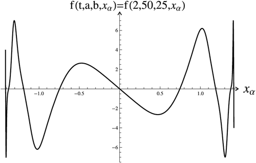
For initial conditions $x(-1)=x_{\gamma }$, $x{ }^{\mathrm{\prime }}(-1)=0$, $0<x_{\gamma }<2$ the number of solutions of BVP (36), (2) is four and for initial conditions $x(-1)=x_{\gamma }$, $x{ }^{\mathrm{\prime }}(-1)=0$, $-1<x_{\gamma }<0$ there are also four solutions to the problem (36), (2), totally eight solutions. By Theorem 1, this is the case for $i=4$ (namely $\frac{4\pi }{2}<\sqrt{50}<\frac{5\pi }{2}$) in the inequality (7). But the number of solutions to the problem (36), (2) can be determined using the formula (11) where $x_0$ is replaced by $x_{\gamma }$ and $t\to t+1$. We have equation

$f(2,50,25,x_{\gamma })=\frac{\sqrt{50(x_2-x_1)}}{\sqrt{3}}(x_{\gamma }-x_1)k^2\mathrm{c}\mathrm{d}\left(2\sqrt{\frac{25(x_2-x_1)}{6}};k\right)\times$

(37) $\times \mathrm{n}\mathrm{d}\left(2\sqrt{\frac{25(x_2-x_1)}{6}};k\right)\mathrm{s}\mathrm{d}\left(2\sqrt{\frac{25(x_2-x_1)}{6}};k\right)=0,\mathrm{w}\mathrm{h}\mathrm{e}\mathrm{r}\mathrm{e}k=\sqrt{\frac{x_{\gamma }-x_1}{x_2-x_1}},$(37)

$x_{1,2}=1.5-0.5x_{\gamma }\mp 0.5\sqrt{3(3-x_{\gamma })(1+x_{\gamma })}$. The graph of $f(2,50,25,x_{\gamma })$ is depicted in Figure 3, Figure 4. There are eight zeros of (37) and, respectively, eight initial values $x_{\gamma }$ which have solutions to the problem (36), (2) ($x_{\gamma }\approx -0.9999989;-0.99986;-0.9835;-0.786$, $x_{\gamma }\approx 1.11319;1.77377;1.9795;1.99998$).

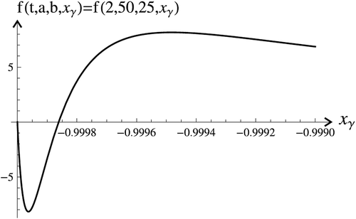
Figure 3. The graph of $f(2,50,25,x_{\gamma })$ for quadratic equation, with eight zeros in $(-1,2)$

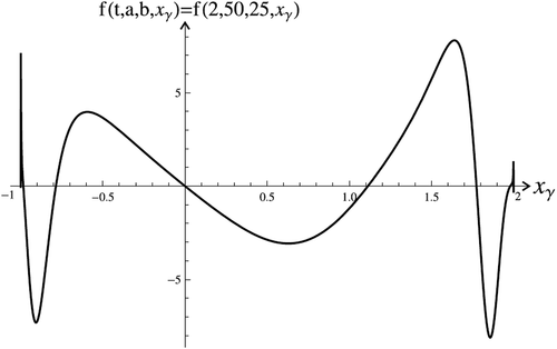
Figure 4. The magnification of the graph of $f(2,50,25,x_{\gamma })$ for quadratic equation, $x_{\gamma }\in [-1,-0.999)$, $x_{\gamma }\approx -0.9999989;-0.99986$

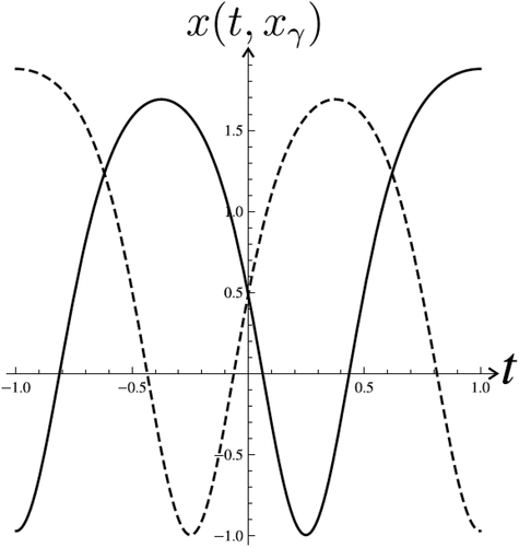
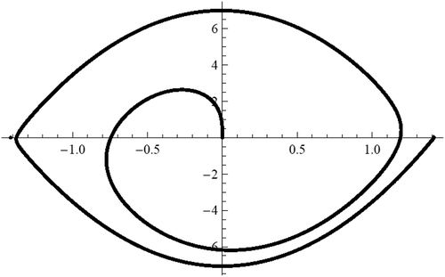
In Figures 5 and 6 we see the behaviors of curves of end-points (at $t=1)$ for equation (36). The curve of values $(x(1,x_{\gamma }),x{ }^{\mathrm{\prime }}(1,x_{\gamma }))$ for equation (36) is a spiral around the origin. Any point of intersection of these curves with the axis $x{ }^{\mathrm{\prime }}=0$ corresponds to a solution of the BVP (36), (2).

Figure 5. Curve $(x(1,x_{\gamma }),x{ }^{\mathrm{\prime }}(1,x_{\gamma }))$ for equation (36), $0<x_{\gamma }<2$

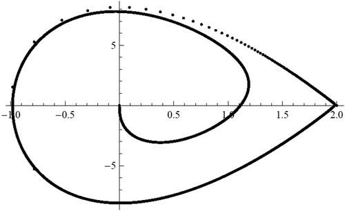
Figure 6. Curve $(x(1,x_{\gamma }),x{ }^{\mathrm{\prime }}(1,x_{\gamma }))$ for equation (36), $-1<x_{\gamma }<0$

Example 2 Consider equation (1), $\phi (x)=x^2$ with $a=50$, $q(t)=b=25$:

(38) $x{ }^{\mathrm{\prime }}{ }^{\mathrm{\prime }}=-50x+25x^3.$(38)

Consider differential equation (38), where the initial conditions are $x(-1)=x_{\alpha }$, $x{ }^{\mathrm{\prime }}(-1)=0$, $0<x_{\alpha }<\sqrt{2}$, then the number of solutions satisfying the boundary conditions (2) is four and for initial conditions $x(-1)=x_{\alpha }$, $x{ }^{\mathrm{\prime }}(-1)=0$, $-\sqrt{2}<x_{\alpha }<0$ there are also four solutions to the problem, totally eight solutions. Therefore, the Theorem 2 is fulfilled. This is the case for $i=4$ (namely $\frac{4\pi }{2}<\sqrt{50}<\frac{5\pi }{2}$) in the inequality (9). On the other hand, the number of solutions to the problem (38), (2) can be determined using the formula (25) and the replacement $t\to t+1$. We get equation

(39) $\begin{array}{rl}& f(2,50,25,x_{\alpha })=\frac{x_{\alpha }\sqrt{50-25x_{\alpha }^2}}{\sqrt{2}}\\ & (k^2-1)\mathrm{n}\mathrm{d}\left(2\sqrt{50-\frac{25}{2}{x}_{\alpha }^2};k\right)\\ & \mathrm{s}\mathrm{d}\left(2\sqrt{50-\frac{25}{2}{x}_{\alpha }^2}t;k\right)=0,\end{array}$(39)

where $k=\sqrt{\frac{25x_{\alpha }^2}{100-25x_{\alpha }^2}}.$ The graph of $f(2,50,25,x_{\alpha })$ is depicted in Figure 7. There are eight zeros of (39) and, respectively, eight initial values $x_{\alpha }$, which have solutions to the problem (38), (2).

Therefore, Proposition 1 is fulfilled.

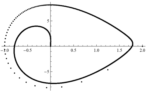
Figure 7. The graph of $f(2,50,25,x_{\alpha })$ for cubic equation in $(-\sqrt{2},\sqrt{2})$

In Figures 8 and 9 we see the behaviours of curves of end-points (at $t=1)$ for equation (38). The curve of values $(x(1,x_{\alpha }),x{ }^{\mathrm{\prime }}(1,x_{\alpha }))$ for equation (38) is a spiral around the origin. Any point of intersection of these curves with the axis $x{ }^{\mathrm{\prime }}=0$ corresponds to a solution of the BVP (38), (2).

Figure 8. Curve $(x(1,x_{\alpha }),x{ }^{\mathrm{\prime }}(1,x_{\alpha }))$ for equation (38), $0<x_{\alpha }<\sqrt{2}$

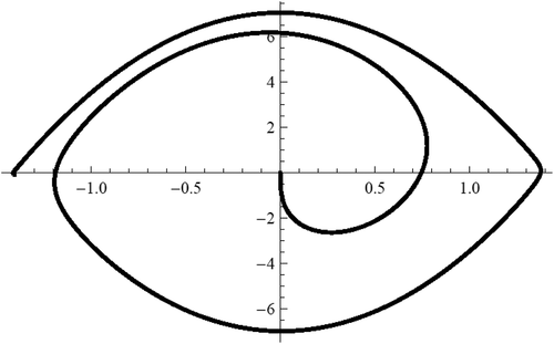
Figure 9. Curve $(x(1,x_{\alpha }),x{ }^{\mathrm{\prime }}(1,x_{\alpha }))$ for eEquation (38), $-\sqrt{2}<x_{\alpha }<0$

Example 3 Consider equation (1), $\phi (x)=x$ with $a=50$, $b=25$:

(40) $x{ }^{\mathrm{\prime }}{ }^{\mathrm{\prime }}=-50x+q(t)x^2,q(t)=\left\{\begin{array}{c}25,t\in [-1,-1+\delta ]=:I_1,\\ 0,t\in (-1+\delta ,1-\delta )=:I_2,\\ 25,t\in [1-\delta ,1]=:I_3,b>0,0<\delta <1.\end{array}\right.$(40)

In what follows we are changing the parameter $\delta$ in this way regulating the width of the interval $I_2.$ We are tracing changes in the number of solutions of BVP and discussing reasons for that. We have observed that for $\delta =0.98$ the number of solutions is five, which is less as predicted by Theorem 1 ($i=4$, $\frac{4\pi }{2}<\sqrt{50}<\frac{5\pi }{2}$).

If $\delta =1$ and the initial conditions are $x(-1)=x_{\alpha }$, $x{ }^{\mathrm{\prime }}(-1)=0$, $-1<x_{\alpha }<2$, $x_{\alpha }\ne 0$, then equation (40) is equation with quadratic nonlinearity $x{ }^{\mathrm{\prime }}{ }^{\mathrm{\prime }}=-50x+25x^2$ and the number of solutions satisfying the boundary conditions (2) is $8$. This was discussed in Example 1.

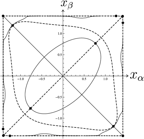
Now we look for solutions of the system (23) which are represented by intersection points of graphs $\mathrm{\Psi }(x_{\gamma },x_{\alpha })$ (dashed line) and $\mathrm{\Phi }(x_{\gamma },x_{\alpha })$ (solid line) (Figure 10). Let $\delta =0.98$. There are totally 5 intersection points of graphs $\mathrm{\Phi }(x_{\gamma },x_{\alpha })$ and $\mathrm{\Phi }(x_{\gamma },x_{\alpha })$ that coresponds to 5 pairs of solutions of BVP (40), (2). These solutions are depicted in Figure 11, Figure 12 and Figure 13, but corresponding points in the Figure 10 are marked.

In this case, coefficient $a$ is large enough but the number of nontrivial solutions is less than $2i$. For $a=50$, $i=4$ the number of solutions as by Theorem 1 should be 8, but there are 5 solutions. Figures 14 and 15 provide explanation of this situation. The curve of end values $(x(1,x_{\gamma }),x{ }^{\mathrm{\prime }}(1,x_{\gamma }))$ for equation (40) leave the region G2 and therefore the number of solutions has decreased.

Figure 10. The trajectory of $\mathrm{\Psi }=0$ (dashed), $\mathrm{\Phi }=0$ (solid), the points which correspond to solutions of system (23) and to the problem (40), (2), $\delta =0.98$

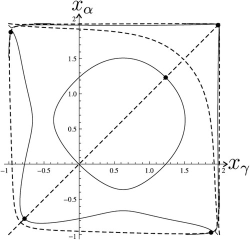
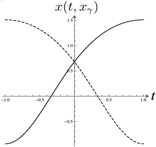
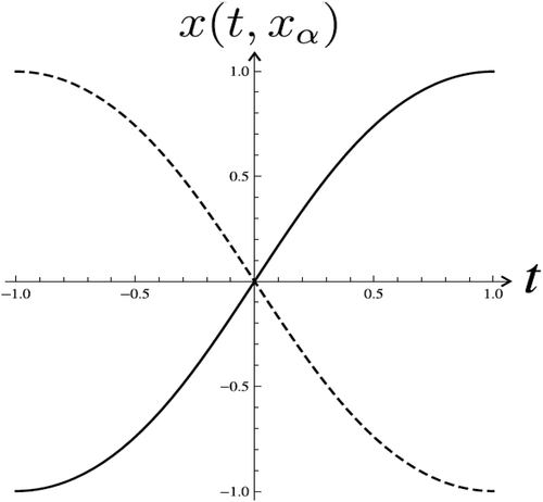
Figure 11. The solutions which correspond to the points $(1.23398,1.23398)$, $x_{\gamma }\approx 1.23398$ (solid) and $(-0.774727,-0.774727)$, $x_{\gamma }\approx -0.774727$ (dashed) in Figure 10, $\delta =0.98$

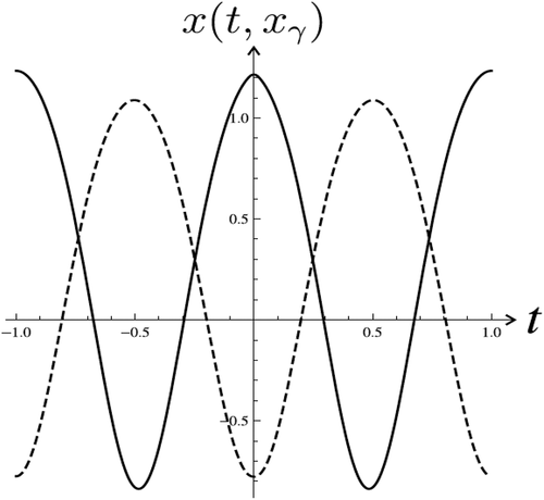
Figure 12. The solution which correspond to the point $(1.97856,1.97856)$, $x_{\gamma }\approx 1.97856$ (solid) in Figure 10, $\delta =0.98$

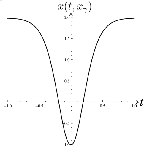
Figure 13. The solutions which correspond to the points $(-0.970911,1.87886)$, $x_{\alpha }\approx -0.970911$ (solid) and $(1.17886,-0.970911)$, $x_{\alpha }\approx 1.17886$ (dashed) in Figure 10, $\delta =0.98$

In Figures 14 and 15 we see the behaviors of curves of end-points (at $t=1)$ for equation (40). The curve of values $(x(1,x_{\gamma }),x{ }^{\mathrm{\prime }}(1,x_{\gamma }))$ for equation (40) is more complicated spiral-like curve than that for quadratic equation (36) (see Figures 5 and 6). Any point of intersection of these curves with the axis $x{ }^{\mathrm{\prime }}=0$ corresponds to a solution of the BVP (40), (2). Figures 14 and 15 show that there are fewer intersections points with the axis $x{ }^{\mathrm{\prime }}=0$ than in the corresponding quadratic equation (36).

Figure 14. Curve $(x(1,x_{\gamma }),x{ }^{\mathrm{\prime }}(1,x_{\gamma }))$ for equation (40), $0<x_{\gamma }<2$, $\delta =0.98$

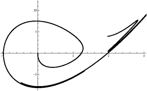
Figure 15. Curve $(x(1,x_{\gamma }),x{ }^{\mathrm{\prime }}(1,x_{\gamma }))$ for equation (40), $-1<x_{\gamma }<0$, $\delta =0.98$

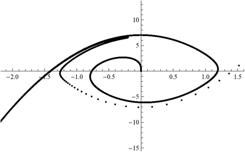
Example 4 Consider equation (1), $\phi (x)=x^2$ with $a=50$, $b=25$:

(41) $x{ }^{\mathrm{\prime }}{ }^{\mathrm{\prime }}=-50x+q(t)x^3,q(t)=\left\{\begin{array}{c}25,t\in [-1,-1+\delta ]=:I_1,\\ 0,t\in (-1+\delta ,1-\delta )=:I_2,\\ 25,t\in [1-\delta ,1]=:I_3,b>0,0<\delta <1.\end{array}\right.$(41)

In what follows we are changing the parameter $\delta$ which regulates the width of the interval $I_2.$ We have observed that for $\delta =0.98$ the number of solutions is greater than eight as predicted by Theorem 2 ($i=4$, $\frac{4\pi }{2}<\sqrt{50}<\frac{5\pi }{2}$).

If $\delta =1$ and the initial conditions are $x(-1)=x_{\alpha }$, $x{ }^{\mathrm{\prime }}(-1)=0$, $-\sqrt{2}<x_{\alpha }<\sqrt{2}$, $x_{\alpha }\ne 0$, then equation (34) is equation with cubic nonlinearity $x{ }^{\mathrm{\prime }}{ }^{\mathrm{\prime }}=-50x+25x^3$ and the number of solutions satisfying the boundary conditions (2) is $8$. This was discussed in Example 2.

Let $\delta =0.98$. Now we look for solutions of the system (34) which are represented by intersection points of graphs ${\mathrm{\Psi }}_1(x_{\alpha },x_{\beta })$ (solid line) and ${\mathrm{\Phi }}_1(x_{\alpha },x_{\beta })$ (dashed line) (Figure 16).

Figure 16. The trajectory of ${\mathrm{\Psi }}_1=0$ (solid), ${\mathrm{\Phi }}_1=0$ (dashed), the points which correspond to solutions of system (34) and to the problem (41), (2), $\delta =0.98$

There are totally 12 intersection points of graphs ${\mathrm{\Psi }}_1(x_{\alpha },x_{\beta })$ and ${\mathrm{\Phi }}_1(x_{\alpha },x_{\beta })$ that coresponds to 12 pairs of solutions of BVP (41), (2). These solutions are depicted in Figure 17, 18, 19, 20, 21 and 22, but the corresponding points in Figure 16 are marked.

Figure 17. The solutions which correspond to the points $(0.766869,0.766869)$, $x_{\alpha }\approx 0.766869$ (solid) and $(-0.766869,-0.766869)$, $x_{\alpha }\approx -0.766869$ (dashed) in Figure 16, $\delta =0.98$

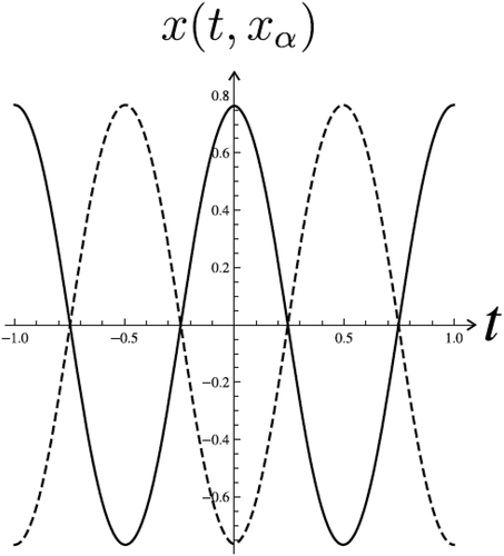
Figure 18. The solutions which correspond to the points $(-1.18879,1.18879)$, $x_{\alpha }\approx -1.18879$ (solid) and $(1.18879,-1.18879)$, $x_{\alpha }\approx 1.18879$ (dashed) in Figure 16, $\delta =0.98$

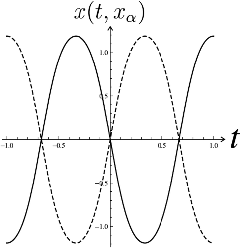
Figure 19. The solutions which correspond to the points $(1.25308,1.4136)$, $x_{\alpha }\approx 1.25308$ (solid) and $(-1.25308,-1.4136)$, $x_{\alpha }\approx -1.25308$ (dashed) in Figure 16, $\delta =0.98$

Figure 20. The solutions which correspond to the points $(1.40795,1.40795)$, $x_{\alpha }\approx 1.40795$ (solid) and $(-1.40795,-1.40795)$, $x_{\alpha }\approx -1.40795$ (dashed) in Figure 16, $\delta =0.98$

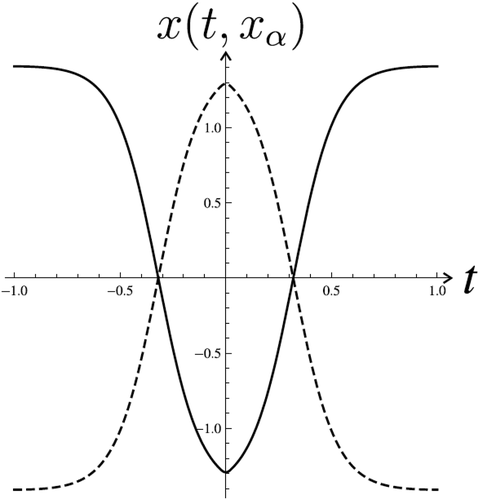
Figure 21. The solutions which correspond to the points $(1.4136,1.25308)$, $x_{\alpha }\approx 1.4136$ (solid) and $(1.4136,-1.25308)$, $x_{\alpha }\approx -1.4136$ (dashed) in Figure 16, $\delta =0.98$

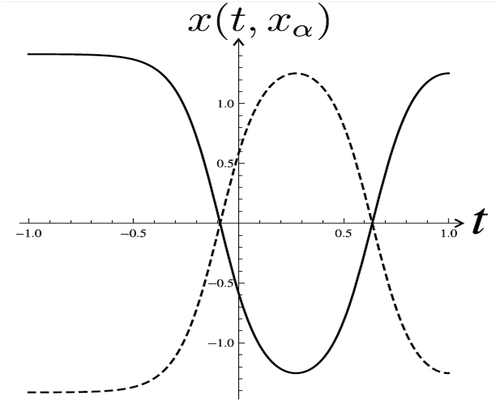
Figure 22. The solutions which correspond to the points $(-1.41396,1.41396)$, $x_{\alpha }\approx -1.41396$ (solid) and $(1.41396,-1.41396)$, $x_{\alpha }\approx 1.41396$ (dashed) in Figure 16, $\delta =0.98$

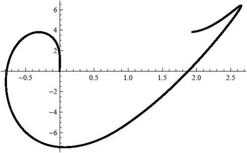
In this case, coefficient $a$ is large enough and the number of nontrivial solutions is greater than $2i$. For $a=50$, $i=4$ the number of solutions for Equation (41) must be 8, but there are 12 for Equation (41).

In Figures 23 and 24 we see the behaviors of curves of end-points (at $t=1)$ for equation (41), where we can see how the additional solutions arise. The curve of values $(x(1,x_{\alpha }),x{ }^{\mathrm{\prime }}(1,x_{\alpha }))$ for equation (41) is more complicated spiral-like curve than for cubic equation (38) (see Figures 8 and 9). Any point of intersection of these curves with the axis $x{ }^{\mathrm{\prime }}=0$ corresponds to a solution of the BVP (41), (2).

Figure 23. Curve $(x(1,x_{\alpha }),x{ }^{\mathrm{\prime }}(1,x_{\alpha }))$ for equation (41), $0<x_{\alpha }<\sqrt{2}$, $\delta =0.98$

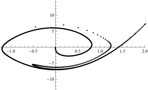
Figure 24. Curve $(x(1,x_{\alpha }),x{ }^{\mathrm{\prime }}(1,x_{\alpha }))$ for equation (41), $-\sqrt{2}<x_{\alpha }<0$, $\delta =0.98$

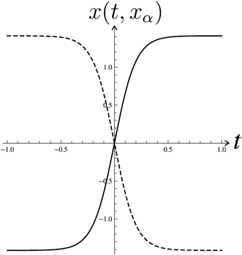
Example 5 Consider equation (1), $\phi (x)=x$ with $a=4$, $b=2$:

(42) $x{ }^{\mathrm{\prime }}{ }^{\mathrm{\prime }}=-4x+q(t)x^2,q(t)=\left\{\begin{array}{c}2,t\in [-1,-1+\delta ]=:I_1,\\ 0,t\in (-1+\delta ,1-\delta )=:I_2,\\ 2,t\in [1-\delta ,1]=:I_3,b>0,0<\delta <1.\end{array}\right.$(42)

.

We have observed that for $\delta =0.98$ the number of solutions is the same as predicted by Theorem 1—two solutions ($i=1$, $\frac{\pi }{2}<\sqrt{4}<\frac{2\pi }{2}$).

If $\delta =1$ and the initial conditions are $x(-1)=x_{\gamma }$, $x{ }^{\mathrm{\prime }}(-1)=0$, $-1<x_{\gamma }<2$, $x_{\gamma }\ne 0$, then equation (23) is equation with quadratic nonlinearity $x{ }^{\mathrm{\prime }}{ }^{\mathrm{\prime }}=-4x+2x^2$ and the number of solutions satisfying the boundary conditions (2) is $2$.

Let $\delta =0.98$. Now we look for solutions of the system (23) which are represented by intersection points of graphs $\mathrm{\Psi }(x_{\gamma },x_{\alpha })$ (solid line) and $\mathrm{\Phi }(x_{\gamma },x_{\alpha })$ (dashed line) (Figure 25).

Figure 25. The trajectory of $\mathrm{\Psi }=0$ (solid), $\mathrm{\Phi }=0$ (dashed), the points which correspond to solutions of system (23) and to the problem (42), (2), $\delta =0.98$

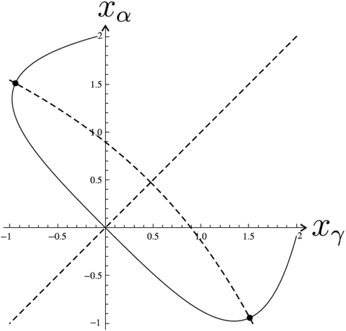
Figure 26. The solutions which correspond to the points $(-0.942088,1.51109)$, $x_{\gamma }\approx -0.942088$ (solid) and $(1.51109,-0.942088)$, $x_{\gamma }\approx 1.51109$ (dashed) in Figure 25, $\delta =0.98$

These solutions are depicted in Figure 26. In this case coefficient $a$ is small enough and the number of nontrivial solutions is $2i$. For $a=4$, $i=1$ the number of solutions must be two.

Example 6 Consider Equation (1), $\phi (x)=x^2$ with $a=4$, $b=2$:

(43) $x{ }^{\mathrm{\prime }}{ }^{\mathrm{\prime }}=-4x+q(t)x^3,q(t)=\left\{\begin{array}{c}2,t\in [-1,-1+\delta ]=:I_1,\\ 0,t\in (-1+\delta ,1-\delta )=:I_2,\\ 2,t\in [1-\delta ,1]=:I_3,b>0,0<\delta <1.\end{array}\right.$(43)

.

We have observed that for $\delta =0.98$ the number of solutions is the same as predicted by Theorem 2, namely, two solutions ($i=1$, $\frac{\pi }{2}<\sqrt{4}<\frac{2\pi }{2}$).

If $\delta =1$ and the initial conditions are $x(-1)=x_{\alpha }$, $x{ }^{\mathrm{\prime }}(-1)=0$, $-\sqrt{2}<x_{\alpha }<\sqrt{2}$, $x_{\alpha }\ne 0$, then Equation (34) is equation with cubic nonlinearity $x{ }^{\mathrm{\prime }}{ }^{\mathrm{\prime }}=-4x+2x^3$ and the number of solutions satisfying the boundary conditions (2) is $2$.

This estimate is in agreement with Theorem 2. Next, let us consider the case $\delta <1$.

Let $\delta =0.98$. Now we look for solutions of the system (34) which are represented by intersection points of graphs ${\mathrm{\Psi }}_1(x_{\alpha },x_{\beta })$ (solid line) and ${\mathrm{\Phi }}_1(x_{\alpha },x_{\beta })$ (dashed line) (Figure 27).

Figure 27. The trajectory of ${\mathrm{\Psi }}_1=0$ (solid), ${\mathrm{\Phi }}_1=0$ (dashed), the points which correspond to solutions of system (34) and to the problem (43), (2), $\delta =0.98$

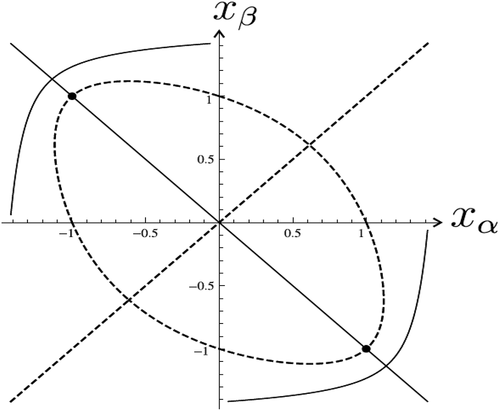
Figure 28. The solutions which correspond to the points $(-0.998339,0.998339)$, $x_{\alpha }\approx -0.998339$ (solid) and $(0.998339,-0.998339)$, $x_{\alpha }\approx 0.998339$ (dashed) in Figure 27, $\delta =0.98$

These solutions are depicted in Figure 28. In this case coefficient $a$ is small enough and the number of nontrivial solutions is $2i$. For $a=4$, $i=1$ the number of solutions must be two.

5. Concluding discussion

In this paper, we investigated the BVP $x{ }^{\mathrm{\prime }}{ }^{\mathrm{\prime }}=-ax+q(t)x\phi (x)$, where $\phi (x)=x$ or $\phi (x)=x^2$, $x{ }^{\mathrm{\prime }}(-1)=x{ }^{\mathrm{\prime }}(1)=0$ with step-wise function $q(t)$ given in (3). The systems that produce the solutions of the BVP (1), (2) are given for both cases of the function $\phi (x)$: $\phi (x)=x$ or $\phi (x)=x^2$. Using the possibilities the instruments of Wolfram Mathematica, the trajectories of those systems are constructed. Therefore, it is possible to determine the number of solutions to the problem and the initial values of solutions. This can be observed in Example 4 and Example 4. These examples show two ways to determine the number of BVP solutions. One of them uses the above-mentioned system, the second one uses behavior of curves of endpoints.

Example 1 and Example 2 consider BVP, where equations contain only quadratic and cubic nonlinearities. This example shows that the number of solutions to BVP can be estimated in three ways and the results obtained are the same. One of them is using results of Theorem 1 or Theorem 2 accordingly to inequality (7) or (9). The second way is to use the graph of exact solution (10) or (24) obtained in the author’s works (Kirichuka & Sadyrbaev, 2019), (Kirichuka, 2019). The third way is using the behavior of curves of end points.

In Example 5 and Example 6 the estimates of the number of solutions for the BVP (1), (2) are obtained for small enough coefficient $a$ and it was shown that the number of solutions is the same as in Theorem 1 or Theorem 2.

Despite the fact that the equation of quadratic nonlinearity looks simpler, finding a solution is more difficult. This can be explained by the fact that for cubic nonlinearity the solution trajectory in the phase plane is symmetric in all four quadrants, but for quadratic nonlinearity this is not the case.

Further research in the indicated direction can be conducted taking into account the following. More polynomial right hand sides $f(x)$ can be studied. The period annuli surrounding critical points appear often in theoretical research and in applications. The trajectories that escape regions like G2 go away and can tend to infinity. The reason is the step-wise character of the coefficient $q(t).$ Therefore the study of such resonant behaviour is possible. Evidently, this can be of practical value. Adding the damping terms of the form $f(x)x{{ }^{\mathrm{\prime }}}^2$ in the equation allows to consider more general cases. Certain transformations of dependent variables can reduce problems with damping to equations of the form studied here. The functions $f(x)$ can be considered which are not polynomials, but the equations have similar properties to what was studied in this paper.

Acknowledgements

The author would like to sincerely thank Professor Felix Sadyrbaev for his useful comments.

Disclosure statement

No potential conflict of interest was reported by the author(s).

Additional information

Funding

The author received no direct funding for this research.

Appendix

We provide below the Wolfram Mathematica codes for several functions and expressions appearing in our paper.

In Figure 29 the code of the function ${\mathrm{\Phi }}_1$ in (33) first equation is given, in code replaced ${\mathrm{\Phi }}_1$ to $\mathrm{\Phi }$, $u=x_{\alpha }$, $v=x_{\beta }$.

${\mathrm{\Phi }}_1$

In Figure 30 the code of the function ${\mathrm{\Psi }}_1$ in (33) second equation is given, in code replaced ${\mathrm{\Psi }}_1$ to $\mathrm{\Psi }$, $u=x_{\alpha }$, $v=x_{\beta }$.

${\mathrm{\Psi }}_1$

In Figure 31 the code of the system (34) for Example 4 is given, simplifying the notation ${\mathrm{\Psi }}_1$ to $\mathrm{\Psi }$, $u=x_{\alpha }$, $v=x_{\beta }$.

In Figure 32 the code for the parametrically defined curve of the values $(x(1,x_{\gamma }),x{ }^{\mathrm{\prime }}(1,x_{\gamma }))$ for the equation (38) is given.

$(x(1,x_{\gamma }),x{ }^{\mathrm{\prime }}(1,x_{\gamma }))$

References

- Beléndez, A., Arribas, E., Beléndez, T., Pascual, C., Gimeno, E., & Álvarez, M. L. (2017). Closed-form exact solutions for the unforced quintic nonlinear oscillator. In Advances in mathematical physics. Hindawi.
- Beléndez, A., Beléndez, T., Martinez, F. J., Pascual, C., Alvarez, M. L., & Arribas, E. (2016). Exact solution for the unforced Duffing oscillator with cubic and quintic nonlinearities. Nonlinear Dynamics, 86(3), 1687–24. https://doi.org/https://doi.org/10.1007/s11071-016-2986-8
- Beléndez, A., Bernabeu, G., Francés, J., Méndez, D. I., & Marini, S. (2010). An accurate closed-form approximate solution for the quintic Duffing oscillator equation. Mathematical and Computer Modelling, 52(3–4), 637–641. https://doi.org/https://doi.org/10.1016/j.mcm.2010.04.010
- Chicone, C. (1987).The monotonicity of the period function for planar Hamiltonian vector fields. Journal of Differential Equations, 69(3), 310321. MR903390;. https://doi.org/https://doi.org/10.1016/0022-0396(87)90122-7
- Chicone, C. (1988). Geometric Methods for Two-Point Nonlinear Boundary Value Problems. Journal of Differential Equations, 72(2), 360–407. https://doi.org/https://doi.org/10.1016/0022-0396(88)90160-X
- Elías-Zúñiga, A. (2013). Exact solution of the cubic-quintic Duffing oscillator. Applied Mathematical Modelling, 37(4), 2574–2579. https://doi.org/https://doi.org/10.1016/j.apm.2012.04.005
- Ellero, E., & Zanolin, F. (2013). Homoclinic and heteroclinic solutions for a class of second-order non-autonomous ordinary differential equations: Multiplicity results for stepwise potentials. Boundary Value Problems, 2013(1), 167. https://doi.org/https://doi.org/10.1186/1687-2770-2013-167
- Gradshteyn, I. S., & Ryzhik, I. M. (2000). Table of Integrals. Series and Products, Academic Press, San Diego, Calif, USA. 6th edition. https://booksite.elsevier.com/samplechapters/9780123736376/Sample_Chapters/01~Front_Matter.pdf
- Gritsans, A., & Sadyrbaev, F. (2015). Extension of the example by Moore-Nehari . Tatra Mt. Math. Publ., 63, 115-127. https://doi.org/https://doi.org/10.1515/tmmp-2015-0024
- Kirichuka, A. (2013). Multiple solutions for nonlinear boundary value problems of ODE depending on two parameters. Proceedings of IMCS of University of Latvia, 13, 83–97. https://protect-us.mimecast.com/s/vOlrCERZP5flWgPkXIPw49I?domain=lumii.lv
- Kirichuka, A. (2016). On the Dirichlet boundary value problem for a cubic on two outer intervals and linear in the internal interval differential equation. Proceedings of IMCS of University of Latvia, 16, 54–66. https://lumii.lv/uploads/sadirbajevs_2016/Sbornik-2016english.htm
- Kirichuka, A. (2017). The number of solutions to the Neumann problem for the second order differential equation with cubic nonlinearity. Proceedings of IMCS of University of Latvia, 17, 44–51. https://lumii.lv/uploads/sadirbajevs_2018/Sbornik2018english.html
- Kirichuka, A. (2018). The number of solutions to the Dirichlet and mixed problem for the second order differential equation with cubic nonlinearity. Proceedings of IMCS of University of Latvia, 18, 63–72. https://lumii.lv/uploads/sadirbajevs_2017/Sbornik2017english.html
- Kirichuka, A. (2019). The number of solutions to the boundary value problem for the second order differential equation with cubic nonlinearity. WSEAS Transactions on Mathematics, 18(31), 230–236. https://lumii.lv/uploads/sadirbajevs_2019/Sbornik2019english.html
- Kirichuka, A. (2020). The number of solutions to the boundary balue broblem with linear-quintic and linear-cubic-quintic nonlinearity. WSEAS Transactions on Mathematics, 19(64), 589–597. https://doi.org/https://doi.org/10.37394/23206.2020.19.64
- Kirichuka, A., & Sadyrbaev, F. (2018a). On boundary value problem for equations with cubic nonlinearity and step-wise coefficient. Differential Equations and Applications, 10(4), 433–447. https://doi.org/https://doi.org/10.7153/dea-2018-10-29
- Kirichuka, A., & Sadyrbaev, F. (2018b). Remark on boundary value problems arising in Ginzburg-Landau theory. WSEAS Transactions on Mathematics, 17, 290–295. https://www.wseas.org/multimedia/journals/mathematics/2018/a685106-1057.php
- Kirichuka, A., & Sadyrbaev, F. (2019). On the number of solutions for a certain class of nonlinear second-order boundary-value problems. Itogi Nauki I Tekhniki. Seriya “Sovremennaya Matematika I Ee Prilozheniya. Tematicheskie Obzory, 160, 32–41. http://www.mathnet.ru/php/archive.phtml?wshow=paper&jrnid=into&paperid=422&option_lang=eng
- Kovacic, I. (2020, August). Nonlinear Oscillations. Springer International Publishing.
- Milne-Thomson, L. M. (1972). Handbook of mathematical functions, chapter 16. In M. Abramowitz & I. A. Stegun (Eds.), Jacobian elliptic functions and theta functions. Dover Publications. http://www.math.ubc.ca/~cbm/aands/abramowitz_and_stegun.pdf
- Moore, R., & Nehari, Z. (1959). Nonoscillation theorems for a class of nonlinear differential equations, Trans. Amer. Math. Soc, 93(1), 30–52. https://doi.org/https://doi.org/10.1090/S0002-9947-1959-0111897-8
- Ogorodnikova, S., & Sadyrbaev, F. (2006). Multiple solutions of nonlinear boundary value problems with oscillatory solutions. Mathematical Modelling and Analysis, 11(4), 413–426. https://doi.org/https://doi.org/10.3846/13926292.2006.9637328
- Shafiq, A., & Hammouch, Z. (2020). Statistical approach of mixed convective flow of third-grade fluid towards an exponentially stretching surface with convective boundary condition. Special Functions and Analysis of Differential Equations, 307, 307–319. https://www.taylorfrancis.com/chapters/edit/ https://doi.org/10.1201/9780429320026-15 /statistical-approach-mixed-convective-flow-third-grade-fluid-towards-exponentially-stretching-surface-convective-boundary-condition-anum-shafiq-zakia-hammouch-tabassum-naz-sindhu-dumitru-baleanu
- Shafiq, A., & Khalique, C. M. (2020). Lie group analysis of upper convected Maxwell fluid flow along stretching surface. Alexandria Engineering Journal, 59(4), 2533–2541. https://doi.org/https://doi.org/10.1016/j.aej.2020.04.017
- Shafiq, A., & Sindhu, T. N. (2017). Statistical study of hydromagnetic boundary layer flow of Williamson fluid regarding a radiative surface. Results in Physics, 7, 3059–3067. https://doi.org/https://doi.org/10.1016/j.rinp.2017.07.077
- Shafiq, A., Sindhu, T. N., & Hammouch, Z. Characteristics of homogeneous heterogeneous reaction on flow of walters’ B liquid under the statistical paradigm. Mathematical Modelling, Applied Analysis and Computation, 272. https://www.researchgate.net/publication/334208119_Characteristics_of_Homogeneous_Heterogeneous_Reaction_on_Flow_of_Walters'_B_Liquid_Under_the_Statistical_Paradigm
- Shang, Y. (2012). A Lie algebra approach to susceptible-infected-susceptible epidemics. Electronic Journal of Differential Equations, 2012(233), 1–7. https://www.researchgate.net/publication/266859292_A_Lie_algebra_approach_to_susceptible-infected-susceptible_epidemics
- Whittaker, E. T., & Watson, G. N. (1996). A course of modern analysis. Cambridge University Press.