Type I error convergence of three hypothesis tests for small RxC contingency tables

ABSTRACT

Many statistical software packages provide hypothesis tests for the independence or association between the rows and columns of a $R\times C$ contingency table. However, insufficient guidance is available about the accuracy and domains-of-validity of some tests that are based on assumptions or approximations. This paper assesses the accuracy of the p-values for three tests of small $R\times C$ tables using Monte Carlo simulations and quantile regression. Results for the Fisher-Freeman-Halton exact tests indicate the p-value accuracy depends on the number of possible unique nominal probabilities. Results for the Pearson chi-square test indicate the p-value accuracy depends on the number of possible unique nominal probabilities and the expected cell counts. Results for the Goodman-Kruskal gamma test indicate the p-value accuracy depends on the number of possible unique ordinal probabilities, the expected cell counts, and the total cell counts. Empirical models for the accuracy of these tests and recommended domain-of-validity criteria are provided.

KEYWORDS:

• Association
• independence
• Monte Carlo simulation
• P-value
• Type I error

Public Interest Statement

Many scientific, technical, and socio-economic fields use contingency tables to evaluate the observed relationships between two or more factors. Statistical tests are widely used to determine whether or not the factors are independent (i.e. no relationship), and whether or not any association between the factors is statistically significant. The results of these tests may affect public policy and legal decisions (e.g. energy, environmental, health, and safety). However, these tests may be based on assumptions and approximations that can affect the accuracy of the test results. Existing guidelines for the use of these tests are often imprecise, inconsistent, subjective, or non-existent. This paper attempts to objectively estimate the accuracy of three exemplar tests and proposes test domain-of-validity criteria based on the estimated accuracy of the tests, which can assist decision-making. The methods developed in this paper can also be applied to other statistical tests and critical test threshold levels.

1. Introduction

Many statistical software packages provide hypothesis tests for the independence (e.g. Pearson chi-square) or association (e.g. Goodman-Kruskal gamma) between the rows and columns of a $R\times C$ contingency table. These tests are often based on assumptions or approximations that may limit their domain-of-validity or accuracy. However, it is unclear from the existing literature and statistical software packages what these limitations are.

This paper assesses the domains-of-validity and accuracy of the Fisher-Freeman-Halton exact (Fisher, 1934; Freeman & Halton, 1951; Mehta & Patel, 1986), the Pearson chi-square (Fleiss, 1981), and the Goodman and Kruskal gamma (Brown & Benedetti, 1977; Goodman & Kruskal, 1979) test p-values for contingency tables up to $4\times 4$ and $2\times 5$ versus indices based on the table dimensions and the row and column margin totals. These three tests were evaluated because they are well known and implemented in several statistical software packages, and the results of which are commonly reported and interpreted by a wide audience. The Fisher–Freeman–Halton test was also included because it is based on the exact reference distribution instead of an approximation.

1.1. Background

1.1.1. R ✕ C contingency tables

Two-dimensional $R\times C$ contingency tables list the frequencies of two discrete data variable value combinations. Given row and column variables with $R$ and $C$ discrete values, let $n_{ij}$ represent the number of times the row variable is equal to the $i$’th discrete value and column variable is equal to the $j$’th discrete value. The result is a table with $R$ rows and $C$ columns. The $i$’th row and $j$’th column margin totals are denoted by $r_i\stackrel{\mathrm{\Delta }}{=}{n}_{i.}$ and $c_j\stackrel{\mathrm{\Delta }}{=}{n}_{.j}$ respectively, where a dot in the subscript denotes summation. The overall total is denoted by $n_{..}$. The expected cell count is ${\hat{n}}_{ij}=r_i{c}_j/n_{..}$.

There are several different tests for the statistical significance of a $R\times C$ table. The appropriateness and accuracy of these tests depends on the type of data, sampling method, sample size, and the null hypothesis ($H_0$) to be tested. The null hypothesis for the Fisher-Freeman-Halton exact and Pearson chi-square tests is the row and column variables are independent or have equal underlying probabilities. The null hypothesis for the Goodman and Kruskal’s gamma test is no association between the row and column variables. Many of these tests are supported by statistical software packages, such as SAS (2013), SPSS (2009), R (R Core Team, 2017; Ekstrøm, 2020), and MATLAB (MathWorks, 2016; Cardillo, 2007a).

1.1.2. Problem statement

We have observed that the Goodman-Kruskal gamma test results for association for some contingency tables appear to be inconsistent with the Pearson chi-square or exact test results for independence (or equal underlying probabilities). For example, consider the $2\times 3$ contingency table in Table 1. The results of three hypothesis tests for this $2\times 3$ table are listed in Table 2. The p-values for the Fisher-Freeman-Halton exact and Pearson chi-square tests are much greater than 0.05, but the p-value for the Goodman-Kruskal gamma test is much less than 0.05.¹ Therefore, these results indicate that there is a statistically significant association between the treatment and outcome even though the null hypothesis for independence or equal underlying probabilities cannot be rejected.²

Table 1. Example $2\times 3$ contingency table

Treatment	Outcome			Total
	X	Y	Z
A	25	8	6	39
B	10	1	0	11
Total	35	9	6	50

Table 2. Hypothesis test results for Table 1

Hypothesis Test	Null Hypothesis ($H_0$)	Alternative Hypothesis	P-value	Reject $H_0$ at the 0.05 level?
Fisher-Freeman-	Equal	Unequal	0.3131	No
Halton	underlying	underlying
	probabilities	probabilities
Pearson	Equal	Unequal	0.2024^a	No
Chi-square	underlying	underlying
	probabilities	probabilities
Goodman-Kruskal	No association	Association	0.0199	Yes
Gamma ($AS{E}_0)$

^aSPSS CROSSTAB results have a footnote indicating ‘3 cells (50.0%) have expected count less than 5. The minimum expected count is 1.32ʹ . The R chi.test function warns the “Chi-squared approximation may be incorrect” .

Existing test guidelines were not sufficient in understanding these apparent inconsistencies (e.g. Table 2). Some recommended criteria for the Pearson chi-square test are that all ${\hat{n}}_{ij}$ should be greater than 5, 10, or even 20. Cochran [Cochran, 1952, p. 328], however, commented that the “numbers 10 and 5 appear to have been arbitrarily chosen”. The SPSS CROSSTAB Pearson chi-square test results for the Example in Table 1 included a footnote “3 cells (50.0%) have expected count less than 5. The minimum expected count is 1.32”. The R chisq.text function presents a warning message for the same table that the “Chi-squared approximation may be incorrect”. However, Cochran indicates in [Cochran, 1954, p. 418] that there are a number of special cases where the ${\chi }^2$ approximation may be adequate if some ${\hat{n}}_{ij}<5$. There is a large body of work that discusses guidelines for using the Pearson chi-square test. Tate and Hyer cited a wide range of opinions in [Tate and Hyer, 1973, p. 836] regarding these guidelines, which are summarized Table 3. Koehler and Larntz observed that “for the null hypothesis of symmetry, the chi-squared approximation for the Pearson statistic is quite adequate at the .05 and .01 nominal levels for expected frequencies as low as .25 when $k\ge 3$, $n\ge 10$, $n^2/k\ge 10$” [Koehler and Larntz, 1980, p. 343].³

Table 3. Example Pearson Chi-Square test recommendations summarized by Tate and Hyer (Tate and Hyer, 1973, p. 836)

Author(s)	Recommendation
Fisher (1934, p. 96)	no ${\hat{n}}_{ij}<5$.
Cramer (1946, p. 420)	all ${\hat{n}}_{ij}\ge 10$.
Kendall (1952, p. 292)	all ${\hat{n}}_{ij}\ge 20$.
Cochran (1954, p. 420)	all ${\hat{n}}_{ij}\ge 1$.
Cochran (1952, p. 329)	a single ${\hat{n}}_{ij}$ can be as low as $1/2$ provided the other ${\hat{n}}_{ij}>$ “the conventional limits of 5 or 10”.
Good et al. (1970, p. 268)	“summarize recommendations of several other writers, all of which tend to be lenient regarding minimum expectations”.

The guidelines for the Goodman-Kruskal gamma test are almost non-existent. Ott et al. indicates, “Although no specific requirement for sample size is generally given, we should never use this test when $n[..]<10$” [Ott et al., 1992, p. 399]. The accuracy of some of these tests for special cases were previously investigated using Monte Carlo methods in (Craddock & Flood, 1970; Göktaş & İşçi, 2011), however clear recommendations regarding the domain-of-validity of the tests were not given.

Therefore, the objective of this study was to assess the domain-of-validity and accuracy of the Fisher–Freeman–Halton, Pearson chi-square, and Goodman-Kruskal gamma tests in order to determine generally applicable guidelines for their use. It was not our objective to evaluate other tests or adjustments, such as the mid p-value (Agresti, 2002) or Ehwerhemuepha (Ehwerhemuepha et al., 2019), which may be more suitable for a given statistical problem.

1.2. Paper organization

The remainder of this paper is organized into five sections. The methods used to are described in Section 2. The results are described in Section 3. Limitations of this analysis are described in Section 4. Recommendations and conclusions are in Sections 5 and 6.

This paper is also accompanied by seven appendices and other supplementary material that are available online. A detailed description of the Monte Carlo simulation method and example results are in Appendix A. Supporting algorithms are described in Appendix B. Empirical envelope model search results are summarized in Appendix C. Supporting methods and results are in Appendix D. Example recommended accuracy criteria calculations are in Appendix E. MATLAB run scripts and functions to reproduce the results herein are described in Appendix F. R run scripts and functions to reproduce the example domain-of-validity and accuracy criteria results herein are described in Appendix G.

2. Methods

The evaluation of the hypothesis test domain-of-validity and accuracy was accomplished in two main steps. First, the 5th percentile p-values for each of the hypothesis tests were estimated for all combinations of $R\times C$ tables within a simulation domain using Monte Carlo simulations (e.g. [Kroese and Chan, 2014, Chapter 7]). This percentile p-value corresponds to the intended critical p-value for the test (e.g. 0.05).⁴ Envelope models to quantify the range of observed 5th percentile p-values based on the table dimensions and row and column margin totals were then determined.

2.1. Monte Carlo simulations

Monte Carlo simulations were used to estimate the 5th percentile p-values ($p_{0.05})$ for contingency tables with independent row and column variables and fixed margin totals (i.e. Method II sampling [Fleiss, 1981, p.27]), for each of the hypothesis tests described in Subsection 2.1.1. This involved first generating a set of randomly sampled contingency tables with independent row and column variables and fixed $r_i$ and $c_j$ margin totals. Then, for each hypothesis test: the p-values for each randomly sampled table were calculated; the empirical distribution of the p-values was determined; and the 5th percentile p-value was calculated; as depicted by the examples in Figure 1. This process is described in more detail in Appendix A. All of the results in this paper were calculated using MATLAB version 9.0 (R2016a) with the Statistics and Machine Learning Toolbox version 10.2 (R2016a) (MathWorks, 2016).

Figure 1. Distributions of observed hypothesis test p-values for a random sample of $2\times 3$ tables with independent row and column variables, $\mathrm{r}=[39,11]$ and $\mathrm{c}=[35,9,6]$

Example cumulative probability distributions of observed p-values from three hypothesis tests of randomly sampled tables are shown in Figure 1. The vertical and horizontal scales of the P–P plots in this figure have been transformed by the cube root of the numerical values to place more emphasis on the smaller probability values that are of interest for hypothesis testing. The cumulative probabilities of the observed values were estimated by the mean rank [Electronics Reliability Subcommittee, 1987, pp.83–84].

Ideally the distribution of calculated p-values for each hypothesis test would be uniformly distributed between 0 and 1 if the null hypothesis is true. Therefore the $\alpha$’th percentile p-value for each test would ideally be $\alpha /100\mathrm{\%}$, and all of the $\circ$ symbols in Figure 1 would ideally be on the diagonal dotted lines. For example, $p_{0.05}$ would ideally be 0.05. The deviation in the observed percentile p-values from the ideal values, as depicted by the $\mathrm{♢}$ symbols in Figure 1 and the solid horizontal line, is the main subject of this analysis.

There are at least two sources of deviation depicted in Figure 1. The first is a staircase effect associated with the discrete number of possible p-values for tables with the same row and column margin totals. This staircase effect is most apparent in Sub Figure 1a for the Fisher-Freeman-Halton exact test, where the sizes of the adjacent steps are about the same, but the overall size trend is increasing, and there are no other sources of error such as asymptotic approximations. The sum of the horizontal step lengths is 1. Therefore, the horizontal length of each step, which represents the minimum and maximum deviation in the observed p-values from the ideal values, tends to be inversely proportional to the number of possible unique p-values (e.g. $|{\mathcal{N}}_{\mathrm{r}\mathrm{c}}|$). The steps for the Fisher-Freeman-Halton test are also to the right of the diagonal line, indicating the observed p-values tend to be equal or greater than the ideal p-value, and therefore the test tends to be conservative.

The second source of deviation from the ideal p-value, which is present in Sub Figure 1b and 1c, but not Sub Figure 1a, is due to the inaccuracy of the assumed reference distribution or asymptotic approximation. This effect is most apparent in Sub Figure 1c, where the calculated p-values between 0.004 and 0.07 tend to be less than the ideal values, based on the assumption that $z_i=G/AS{E}_i$ is normally distributed (see Appendix D.3), and therefore tends to be liberal. Furthermore the extreme tails of the calculated p-value distribution are also truncated in the other direction (i.e. tends to be conservative) because $-1\le G\le 1$. This later condition occurred for one of the observed values in Sub Figure 1c where $G=-1$, $AS{E}_0=0.2785$, and the resulting p-value is 0.000330 (see the first row in Table A1). The example results in Sub Figure 1b suggest that the discrete staircase and asymptotic approximation effects on the Pearson chi-square test p-values have similar magnitudes, and that the overall trend tends to be unbiased.

P-value distributions were calculated for all combinations of the row and column margin totals (i.e. $r_i$ and $c_j$) within the simulation domain summarized in Table 4. This comprised all $R\times C$ tables with $n_{..}$ between the minimum and maximum values listed in columns 3 and 4, inclusive. The $R\times C$ table dimensions comprised $2\le R\le C\le 4$ plus $2\times 5$ tables. Tables with $R>C$ dimensions were not included because the p-values for the hypothesis tests considered herein are same as the transposed table. The $2\times 5$ tables were included to better elucidate potential independent effects of table dimensions and degrees-of-freedom.

Table 4. $R\times C$ contingency table simulation domain

$R$	$C$	Minimum $n_{..}$	Maximum $n_{..}$	Maximum $min\left({\hat{n}}_{ij}\right)$	Number of Table Margin Combinations ${\sum }_{n_{..}}\left(\begin{array}{c}{n}_{..}-1\\ R-1\end{array}\right)\left(\begin{array}{c}{n}_{..}-1\\ C-1\end{array}\right)$	Hypothesis Tests (see key)
2	2	2	200	50	2,646,700	F,P,G
2	3	3	84	14	5,979,071	F,P,G
2	4	4	40	5	2,906,202	F,P,G
2	5	5	30	3	3,538,899	P,G
3	3	3	36	4	2,622,522	F,P,G
3	4	4	27	2.25	3,981,510	P,G
4	4	4	20	1.25	2,904,093	P,G
Total					24,578,997

Key: F—Fisher-Freeman-Halton exact, P—Pearson chi-square, G—Goodman-Kruskal gamma.

The simulation method and example results are described in more detail in Appendix A.

2.1.1. Hypothesis test P-values

P-values for each of the following hypothesis tests were calculated for each unique table:

• Fisher and Fisher-Freeman-Halton exact tests. P-values for $2\times 2$ tables were calculated using the fishertest function in the MATLAB statistics toolbox. P-values for $2\times 3$, $2\times 4$, and $3\times 3$ tables were calculated using Cardillo’s myfisher23, myfisher24, and myfisher33 functions (Cardillo, 2007a, 2007b and 2007c).

• Pearson chi-square test. This test assumes that $X^2={\sum }_{i=1}^R{\sum }_{j=1}^C{\left(n_{ij}-{\hat{n}}_{ij}\right)}^2/{\hat{n}}_{ij}$ has a ${\chi }^2$ distribution with $\nu =(R-1)(C-1)$ degrees-of-freedom if $H_0$ is true. The p-value is the probability of the observed or larger $X^2$ value if $H_0$ is true, which was calculated using the chi2cdf function in the MATLAB statistics toolbox.

This assumption is one of convenience because the “$X^2$ statistic has approximately a chi-square distribution for large samples sizes. It is difficult to specify what ‘large’ means, but $\left\{[{\hat{n}}_{ij}]\ge 5\right\}$ is sufficient” [Agresti, 1996, p. 28]. The accuracy of the p-value resulting from this assumption and approximation is one of the subjects of this study.

• Goodman-Kruskal’s gamma test. There is more than one version of the Goodman-Kruskal gamma test. The original version proposed by Goodman and Kruskal is described in Appendix D.3.2. A modified version based on (Brown & Benedetti, 1977), which is implemented in SAS [SAS, 2013, p. 160] and SPSS [SPSS, 2010, p. 161], is described in Appendix D.3.1. This test assumes that $z_i=G/AS{E}_i$ has a normal distribution with zero mean and unit standard deviation if $H_0$, where $G$ and $AS{E}_i$ are calculated according to the equations in Appendix D.3. The subscript $i$ denotes the modifed ($0$) or original ($3$) version of the test. The p-value is the probability of the observed or larger $|z_i|$ value if $H_0$ is true, which was calculated using the normcdf function in the MATLAB statistics toolbox.

This assumption is also one of convenience because according to (Goodman & Kruskal, 1979) (e.g. pages 78 and 93) and (Brown & Benedetti, 1977), $z_0$ actually has an approximate, asymptotically unit-normal distribution for large $n_{..}$. The $z_i$ value is approximately normally distributed because $G$ is limited to $-1\le G\le 1$. The accuracy of the p-value resulting from this assumption and approximation is also one of the subjects of this study.

2.2. Candidate accuracy assessment envelope models

It is assumed herein that the accuracy of the hypothesis test p-values can vary depending on the contingency table dimensions and the row and column margin totals. Candidate envelope models and indices to quantify this relationship are described is this section.

2.2.1. Candidate quantile models

The accuracy of the hypothesis tests is described herein by the 2.5% and 97.5% quantiles of the observed $p_{0.05}$ values. These quantiles represent the lower bounds ($LB$) and upper bounds ($UB$) of a 95% interval enclosed by the envelope model. Note the 0.0% and 100% quantiles were not used because these quantiles are numerically ill-defined and non-unique. For example, one numerical solution for the 100% quantile of observed $p_{0.05}$ values is simply 1, which is not very descriptive of the upper bounds. It was also generally assumed that the $LB$ and $UB$ will tend to (e.g. asymptotically) converge to the ideal value ($p_{\mathrm{i}\mathrm{d}\mathrm{e}\mathrm{a}\mathrm{l}}$) (e.g. 0.05) as the candidate indices tend towards a limiting value. This limiting value can be either infinity or zero, depending on the type of index. Therefore, the following empirical model forms were considered for the $LB$, $UB$, and median quantiles:

(1) $Q=\pi \left(g\left(p_{\mathrm{i}\mathrm{d}\mathrm{e}\mathrm{a}\mathrm{l}}\right)+\sum _i\sum _j{\beta }_{i,j}{x}_i^{q_{i,j}}\right)+\text{isin}$(1)

(2) $Q=\pi \left(g\left(p_{\mathrm{i}\mathrm{d}\mathrm{e}\mathrm{a}\mathrm{l}}\right)+sexp\left({\lambda }_0+\sum _i{\lambda }_{i}log\left(x_i\right)\right)\right)+\text{isin}$(2)

where $\pi (a)\stackrel{\mathrm{\Delta }}{=}exp\left(a\right)/\left(1+exp\left(a\right)\right)$, $g(b)\stackrel{\mathrm{\Delta }}{=}ln\left(b/\left(1-b\right)\right)$, and $x_i$ are one or more candidate indices. The $q_{i,j}$ in Equation (1)(1) $Q=\pi \left(g\left(p_{\mathrm{i}\mathrm{d}\mathrm{e}\mathrm{a}\mathrm{l}}\right)+\sum _i\sum _j{\beta }_{i,j}{x}_i^{q_{i,j}}\right)+\text{isin}$(1) are assumed polynomial powers for $x_i$. The ${\beta }_{i,j}$ and $\in$ are unknown coefficients to be estimated by quantile regression (e.g. (Grinsted, 2008)). The $s$ coefficient in Equation (2)(2) $Q=\pi \left(g\left(p_{\mathrm{i}\mathrm{d}\mathrm{e}\mathrm{a}\mathrm{l}}\right)+sexp\left({\lambda }_0+\sum _i{\lambda }_{i}log\left(x_i\right)\right)\right)+\text{isin}$(2) is either +1 or −1, and ${\lambda }_i$ and $\in$ are unknown coefficients to be estimated by quantile regression. The form of these equations guarantee that $0<Q<1$ for $x_i>0$ and $Q\to p_{\mathrm{i}\mathrm{d}\mathrm{e}\mathrm{a}\mathrm{l}}$ if all $x_i\to \mathrm{\infty }$ and $q_{i,j}<0$. These two models are equivalent if ${\beta }_{1,1}=exp({\lambda }_0)$, $q_{1,1}={\lambda }_1$, and all other ${\beta }_{i,j}=0$ and ${\lambda }_i=0$.

The polynomial model form in Equation (1)(1) $Q=\pi \left(g\left(p_{\mathrm{i}\mathrm{d}\mathrm{e}\mathrm{a}\mathrm{l}}\right)+\sum _i\sum _j{\beta }_{i,j}{x}_i^{q_{i,j}}\right)+\text{isin}$(1) is well suited for fitting one or more indices simultaneously for assumed ${\mathrm{q}}_i$ values. The assumed values for ${\mathrm{q}}_i$ included [1], [−0.5], [−1], [−1,-2], and [−1,-2,-3] depending on the test and candidate index. Higher degree polynomials can fit the data better than lower degree polynomials, but can result in overparameterized models, which is undesirable.

The logarithmic model form in Equation (2)(2) $Q=\pi \left(g\left(p_{\mathrm{i}\mathrm{d}\mathrm{e}\mathrm{a}\mathrm{l}}\right)+sexp\left({\lambda }_0+\sum _i{\lambda }_{i}log\left(x_i\right)\right)\right)+\text{isin}$(2) is only applicable to a single index but can be used to estimate a scalar value for ${\mathrm{q}}_i$. These models tend to be more parsimonious, which is desirable.

2.2.2. Candidate accuracy assessment indices

Four types of candidate indices based on the table dimensions and margin totals were considered to assess different potential effects on p-value accuracy. The first three types of indices have positive values that tend to increase for tables with larger margin totals or overall counts. The last type of index has a value between 0 and 1.

2.2.2.1. Candidate discreteness indices

The following indices were considered to represent effects of the discrete p-value distribution resulting from the whole number table counts (e.g. as depicted by the staircase shaped curve in Sub Figure 1a):

$\left|{\mathcal{S}}_{\mathrm{r}\mathrm{c}}\right|$ The number of unique $R\times C$ tables with $r_i$ and $c_j$ marginal totals ($|\mathcal{S}|$ in this context denotes the cardinality of set $\mathcal{S}$, and ${\mathcal{S}}_{\mathrm{r}\mathrm{c}}$ is the set of all unique $R\times$ C tables as defined in Appendix b.1) The rationale for this candidate index is that the distribution of sampled p-values depends on the maximum possible number of unique sampled p-values, which is less than or equal to $|{\mathcal{S}}_{\mathrm{r}\mathrm{c}}|$. An algorithm to calculate $|{\mathcal{S}}_{\mathrm{r}\mathrm{c}}|$ given $R$, $C$, and the margin totals is in Appendix B.1. Other algorithms are described in (Diaconis & Gangolli, 1994; Gail & Mantel, 1977).

$|{\mathcal{N}}_{\mathrm{r}\mathrm{c}}|$ The number of unique nominal probabilities for $R\times C$ tables with $r_i$ and $c_j$ marginal totals. The rationale for this index is that the distribution of sampled nominal (e.g. the Fisher-Freeman-Halton exact test) p-values depends on $|{\mathcal{N}}_{\mathrm{r}\mathrm{c}}|$. An algorithm to calculate $|{\mathcal{N}}_{\mathrm{r}\mathrm{c}}|$ given $R$, $C$, and the margin totals is in Appendix B.2. Note that $|{\mathcal{N}}_{\mathrm{r}\mathrm{c}}|\le |{\mathcal{S}}_{\mathrm{r}\mathrm{c}}|$.

$|{\mathcal{O}}_{\mathrm{r}\mathrm{c}}|$ The number of unique ordinal probabilities for $R\times C$ tables with $r_i$ and $c_j$ marginal totals. The rationale for this index is that the distribution of sampled ordinal (e.g. the Goodman-Kruskal gamma test) p-values depends on $|{\mathcal{O}}_{\mathrm{r}\mathrm{c}}|$. An algorithm to calculate $|{\mathcal{O}}_{\mathrm{r}\mathrm{c}}|$ is in Appendix B.3. Note that $|{\mathcal{O}}_{\mathrm{r}\mathrm{c}}|\le |{\mathcal{S}}_{\mathrm{r}\mathrm{c}}|$.

2.2.2.2. Candidate approximation indices

The following indices were also considered for the Pearson chi-square and Goodman and Kruskal gamma tests to represent approximation accuracy and asymptotic standard error effects:

• The minimum expected cell count, which is ${\hat{n}}_{\mathrm{m}\mathrm{i}\mathrm{n}}\stackrel{\mathrm{\Delta }}{=}{min}_{i=1}^R\left({min}_{j=1}^C{\hat{n}}_{ij}\right)$. The rationale for this candidate index is that Fleiss [Fleiss, 1981, p. 25] and others have warned that the Pearson chi-square test may not be accurate if ${\hat{n}}_{\mathrm{m}\mathrm{i}\mathrm{n}}$ is small, (e.g. ${\hat{n}}_{\mathrm{m}\mathrm{i}\mathrm{n}}<$ 5, 10, or 20).

• The sum and the average of the $\nu$ smallest expected cell counts, which are ${\sum }_{\mathrm{m}\mathrm{i}\mathrm{n}}^{\nu }\hat{n}\stackrel{\mathrm{\Delta }}{=}{\sum }_{k=\mathrm{m}\mathrm{i}\mathrm{n}}^{\nu }{\hat{n}}_k$ and ${\sum }_{\mathrm{m}\mathrm{i}\mathrm{n}}^{\nu }\hat{n}/\nu$, where ${\hat{n}}_k$ is the $k$’th smallest expected cell count. The rationale for these indices is that they can account for multiple small expected cell counts in higher dimension tables. These indices are equal to ${\hat{n}}_{\mathrm{m}\mathrm{i}\mathrm{n}}$ for $2\times 2$ tables.

• The harmonic mean and the root harmonic mean of the expected cell counts, which are ${\hat{n}}_{\mathrm{h}\mathrm{m}}\stackrel{\mathrm{\Delta }}{=}RC/\left({\sum }_{i=1}^R{\sum }_{j=1}^C{\hat{n}}_{ij}^{-1}\right)$, and ${\hat{n}}_{\mathrm{r}\mathrm{h}\mathrm{m}\mathrm{s}}\stackrel{\mathrm{\Delta }}{=}\sqrt{RC/\left({\sum }_{i=1}^R{\sum }_{j=1}^C{\hat{n}}_{ij}^{-2}\right)}$. The rationale for these indices is that they can also account for multiple small expected cell counts.

Scaled and offset versions of the candidate expected cell count indices ($x_i$) were also considered (i.e. $A{x}_i+B$). The offset $B=1$ was considered to avoid small numerical values which, when inverted by a negative $q_{i,j}$ power in Equation (1)(1) $Q=\pi \left(g\left(p_{\mathrm{i}\mathrm{d}\mathrm{e}\mathrm{a}\mathrm{l}}\right)+\sum _i\sum _j{\beta }_{i,j}{x}_i^{q_{i,j}}\right)+\text{isin}$(1) , become very large and can adversely affect the overall model fit. Scaling factors $A=\nu$ and $A=RC$ were considered to address potential effects of different contingency table dimensions.

The scaling factor $A=1/f(X_{0.05}^2,\nu )$ was also considered to potentially normalize the effects of different table dimensions on the Pearson chi-square p-values. This scaling factor and values are described in Appendix D.1.

2.2.2.3. Candidate sample size indices

The total table count $n_{..}$ was also considered for the Pearson chi-square and Goodman and Kruskal gamma test envelope models. The rationale is that $n_{..}$ appears in the gamma test based on $AS{E}_0$ but not the original test based on $AS{E}_3$ (see Equations D.3 and D.8). Therefore, the difference between the two gamma test p-values goes to zero if $n_{..}\to 0$. The scaled indices $\nu n_{..}$, $n_{..}/\nu$, $RC{n}_{..}$, and $n_{..}/RC$ were also considered to address potential effects of different contingency table dimensions. Koehler and Larntz (Koehler & Larntz, 1980) also investigated the effects of sample size ($n_{..}$) and the number of cells ($RC$) on the accuracy of the Pearson chi-square approximation.

2.2.2.4. Candidate P-value range indices

The minimum and maximum possible p-values for a given test and row and column margin totals may also be related to the domain-of-validity and the accuracy of the hypothesis test p-values. These indices are denoted by $min\left(p_{\mathrm{t}\mathrm{e}\mathrm{s}\mathrm{t}}\right)$ and $max\left(p_{\mathrm{t}\mathrm{e}\mathrm{s}\mathrm{t}}\right)$. They can be calculated by the algorithms in Appendix B to calculate $|{\mathcal{N}}_{\mathrm{r}\mathrm{c}}|$ and $|{\mathcal{O}}_{\mathrm{r}\mathrm{c}}|$.

In general $min\left(p_{\mathrm{t}\mathrm{e}\mathrm{s}\mathrm{t}}\right)$ tends to approach 0 and $max\left(p_{\mathrm{t}\mathrm{e}\mathrm{s}\mathrm{t}}\right)$ tends to approach 1, for tables with large numerical values. There are two special cases for the Fisher-Freeman-Halton exact test:

• $max\left(p_{\mathrm{F}\mathrm{i}\mathrm{s}\mathrm{h}\mathrm{e}\mathrm{r}}\right)=1$ because the p-value for a given table is defined as the sum of the probabilities for all of the tables with the same $r_i$ and $c_j$ that are as extreme or more extreme as the given table [Fleiss, 1981, p. 25] and [MathWorks, 2016, p. 25–1564]. There will always be at least one extreme table for which this sum includes all of the possible tables.

• $min\left(p_{\mathrm{F}\mathrm{i}\mathrm{s}\mathrm{h}\mathrm{e}\mathrm{r}}\right)=1$ if $|N_{\mathrm{r}c}|=1$ because the sum of the probabilities for the only unique probability is 1.0.⁵

This leads to the following proposed p-value domain-of-validity criterion:

If the critical p-value (e.g. 0.05) is less than $min\left(p_{\mathrm{t}\mathrm{e}\mathrm{s}\mathrm{t}}\right)$ or greater than $max\left(p_{\mathrm{t}\mathrm{e}\mathrm{s}\mathrm{t}}\right)$ then the row and column margin totals are outside the test p-value domain-of-validity for the critical p-value.

This criterion would be in addition to other possible test accuracy criteria to be identified.

The $max\left(p_{\mathrm{t}\mathrm{e}\mathrm{s}\mathrm{t}}\right)$ indices were not considered for the candidate envelope models.

2.2.3. Quantile regression method

Quantile regressions were accomplished using the quantreg3.m function (see the Supplementary Online Material). This function finds the value for $b$ that minimizes fval, defined as

(3) $\mathrm{f}\mathrm{v}\mathrm{a}\mathrm{l}=\sum _k^N\left|{\tilde{y}}_k\left\{\begin{array}{cc}\tau -1& \mathrm{i}\mathrm{f}{\tilde{y}}_k<0\\ \tau & \mathrm{o}\mathrm{t}\mathrm{h}\mathrm{e}\mathrm{r}\mathrm{w}\mathrm{i}\mathrm{s}\mathrm{e}\end{array}\right\}\right|,$(3)

where $\tilde{\mathrm{y}}=\mathcal{F}\left(\mathrm{X}\mathrm{b}\right)-\mathrm{y}$, $\mathrm{y}$ is a $N\times 1$ matrix of $N$ observed dependent variable values (e.g. $p_{0.05}$), $\mathrm{X}$ is a corresponding $N\times p$ matrix of $p$ corresponding independent variable values (e.g. $x_i^{-j}$), $\mathrm{b}$ is an estimate of $\beta$, and $\tau$ is the desired quantile (e.g. 0.025 or 0.975), and $\mathcal{F}$ is an output transformation (e.g. $\mathcal{F}\left(\bullet \right)=\pi \left(\bullet +g(p_{\mathrm{i}\mathrm{d}\mathrm{e}\mathrm{a}\mathrm{l}})\right)$). The quantreg3 function is based on Grinsted’s quantreg.m function (Grinsted, 2008) with the following extensions:

(1) optional input to provide an initial guess for the estimated $\beta$ values (${\mathrm{b}}_0$), otherwise it is assumed that ${\mathrm{b}}_0={\mathrm{X}}^{-1}\mathrm{y}$.

(2) optional input to provide an output transformation function $\mathcal{F}$, otherwise it is assumed that $\mathcal{F}\left(\bullet \right)=\bullet$.

(3) optional output to return the fval value calculated by the fminsearch.m function.

The average difference between the observed and modeled quantile ($\bar{f}$) was then calculated by dividing fval by the number of observations in the regression for candidate model comparison purposes.

The initial guesses for the $LB$ and $UB$ models were

(4) ${\mathrm{b}}_0={\left[\begin{array}{c}\mathrm{X}\\ {\mathrm{I}}_{p\times p}\end{array}\right]}^{-1}\left[\begin{array}{c}\mathrm{y}\\ 0_{p\times 1}\end{array}\right],$(4)

where ${\mathrm{y}}_k=g\left(p_{0.05,k}\right)-g\left(p_{ideal}\right)$, ${\mathrm{I}}_{p\times p}$ is an $p\times p$ identity matrix, and $0_{p\times 1}$ is a $p\times 1$ matrix of zeroes. The $p$ additional rows in Equation (4)(4) ${\mathrm{b}}_0={\left[\begin{array}{c}\mathrm{X}\\ {\mathrm{I}}_{p\times p}\end{array}\right]}^{-1}\left[\begin{array}{c}\mathrm{y}\\ 0_{p\times 1}\end{array}\right],$(4) helps to prevent large ${\mathrm{b}}_0$ values if $\mathrm{X}$ is ill-conditioned. The initial guess for the median model was the average of the estimated $\beta$ values for the $LB$ and $UB$ models.

In some cases, the quantile regression did not converge within the default number of iterations, possibly due to overparameterization. If this occurred then submodels with one or more dropped terms were evaluated, and the submodel yielding in the minimum fmin value was selected. In this case the estimated $\beta$ values for the missing terms were set to 0. As a final step, the quantile regression with all of the candidate terms was reattempted using the best estimated submodel as an initial guess. This was accomplished by the quantreg_s3.m function, which calls the quantreg3.m function (which was in turn based on Grinsted’s quantreg.m function (Grinsted, 2008)).

The 95% confidence intervals for the estimated model coefficients were estimated using the jackknife method described by Kahane [Kahane, 2012, pp. 64–66]. This involved classifying the $p_{0.05}$ observations into (e.g. 14) groups ($k$) based on the $R\times C$ table dimensions and whether or not $n_{..}$ was even or odd. The quantile regression model coefficients were then re-estimated by removing the data for one group $k$ at a time (i.e. ${\mathrm{b}}_{-k}$). Pseudo estimates of the model coefficients (${\mathrm{b}}_k$) were then determined based on ${\mathrm{b}}_{-k}-\mathrm{b}$. The 95% confidence intervals were then estimated based on variation in ${\mathrm{b}}_k$. The rationale for the jackknife grouping is to address potential table dimension sampling effects, and potential effects of “even-size samples” mentioned in [Goodman and Kruskal, 1979, p. 363].

3. Results

Single index trends and envelope model search results for the 5th percentile Fisher-Freeman-Halton exact, Pearson chi-square, and Goodman-Kruskal gamma test p-values are presented in separate subsections.

3.1. Fifth percentile Fisher-Freeman-Halton exact test P-values

3.1.1. Single Index Trends

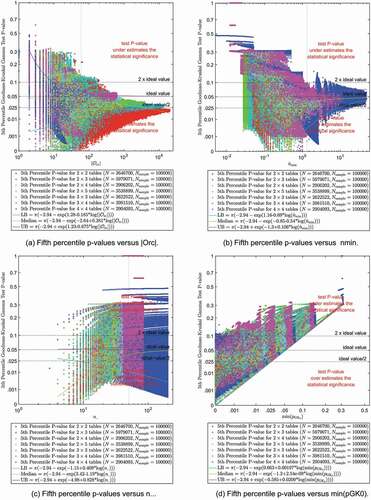
The results in Figure 2 compare the 5th percentile p-values from the Monte Carlo simulations of the Fisher and Fisher-Freeman-Halton exact tests to $|{\mathcal{S}}_{\mathrm{r}\mathrm{c}}|$, $|{\mathcal{N}}_{\mathrm{r}\mathrm{c}}|$, and $min\left(p_{\mathrm{F}\mathrm{i}\mathrm{s}\mathrm{h}\mathrm{e}\mathrm{r}}\right)$ respectively. The results for four different $R\times C$ table dimensions are depicted by different symbol types as indicated in the legend. The number of observed $p_{0.05}$ values for each table dimension are also indicated in the legend. The total number of $p_{0.05}$ observations in each figure is 14,154,495 .⁶ Each of the $p_{0.05}$ observations is based on the p-values from 100,000 randomly sampled tables. Therefore, the results in these figures are based on 1,415,449,500,000 randomly sampled tables. The horizontal dotted lines indicate $1/2$, 1, and 2 times the ideal 5th percentile p-value value (0.05) for reference purposes. Sub Figure 2b also includes a reference curve for $0.05+1/|{\mathcal{N}}_{\mathrm{r}\mathrm{c}}|$, which represents a theoretical maximum deviation from the ideal p-value assuming that the $|{\mathcal{N}}_{\mathrm{r}\mathrm{c}}|$ possible unique p-values are equally spaced.

Figure 2. Fifth percentile Fisher-Freeman-Halton p-values versus $|{\mathcal{S}}_{\mathrm{r}\mathrm{c}}|$, $|{\mathcal{N}}_{\mathrm{r}\mathrm{c}}|$, and $min\left(p_{\mathrm{F}\mathrm{i}\mathrm{s}\mathrm{h}\mathrm{e}\mathrm{r}}\right)$

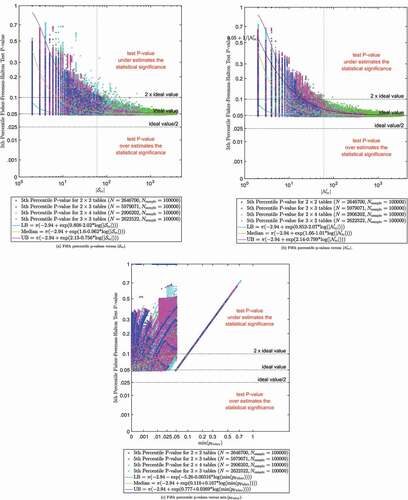
This figure shows that all of the 5th percentile p-values are greater than or equal to 0.05. This indicates that the Fisher-Freeman-Halton exact test tends to be conservative, a result which has been observed by others (e.g. [Agresti, 2002, pp. 93–94]).

The vertical dotted lines indicate the index values for all $2\times 3$ tables with row margins = [39,11] and column margins = [35,9,6] (e.g. Table 1). These subfigures indicate that $p_{0.05}$ tends to be between 0.05 and 0.10 for these index values, which is desirable from a test accuracy viewpoint.⁷

Figure 2 also shows estimated curves for the candidate $UB$, median, and $LB$ models based on Equation (2)(2) $Q=\pi \left(g\left(p_{\mathrm{i}\mathrm{d}\mathrm{e}\mathrm{a}\mathrm{l}}\right)+sexp\left({\lambda }_0+\sum _i{\lambda }_{i}log\left(x_i\right)\right)\right)+\text{isin}$(2) . The equations for the curves are also indicated in the legend. The models were fit to 13,696,372 observed $p_{0.05}$ values for $R\times C$ tables with $min\left(p_{\mathrm{F}\mathrm{i}\mathrm{s}\mathrm{h}\mathrm{e}\mathrm{r}}\right)\le 0.05$. The other 458,123 observations with $min\left(p_{\mathrm{F}\mathrm{i}\mathrm{s}\mathrm{h}\mathrm{e}\mathrm{r}}\right)>0.05$ were excluded because they were outside the 0.05 p-value domain-of-validity for the Fisher-Freeman-Halton exact test. The excluded observations included 475 $p_{0.05}$ values for $R\times C$ tables with $|{\mathcal{N}}_{\mathrm{r}\mathrm{c}}|=1$.

These subfigures indicate the observed $p_{0.05}$ values tend to converge towards the ideal 5th percentile p-value as $|{\mathcal{S}}_{\mathrm{r}\mathrm{c}}|$ or $|{\mathcal{N}}_{\mathrm{r}\mathrm{c}}|$ increases. This result was anticipated based on the example results in Sub Figure 1a, which indicated that the deviation in the observed p-values from the ideal p-values tends to be inversely proportional to the number of possible unique test p-values. The estimated $UB$ curve in Sub Figure 2b tends to follow the theoretical $0.05+1/|{\mathcal{N}}_{\mathrm{r}\mathrm{c}}|$ curve, allowing for differences due to the assumed logistic form of the $UB$ model and variation in unique probability spacing. The range of data and the estimated $LB$ curve indicates that the lower bounds for $p_{0.05}$ are approximately equal to the ideal 5th percentile p-value, which is expected for the exact tests. This result was also anticipated based on Sub Figure 1a, which showed that the observed p-values were greater than or equal to the ideal p-values.

Sub Figure 2c is similar to Sub Figure 2a and 2b with the following exceptions. The candidate index is $min\left(p_{\mathrm{F}\mathrm{i}\mathrm{s}\mathrm{h}\mathrm{e}\mathrm{r}}\right)$. The horizontal axis scale has been transformed to correspond to the vertical axis because they are both probabilities. Sub Figure 2c shows a large number of observations with $min\left(p_{\mathrm{F}\mathrm{i}\mathrm{s}\mathrm{h}\mathrm{e}\mathrm{r}}\right)>0.05$, and therefore outside the test 0.05 p-value domain-of-validity. The observations outside the 0.05 p-value domain-of-validity were not used to fit the candidate envelope models.

Results for the candidate single index models are summarized in Table C.1 in Appendix C. The results are rank ordered from the smallest (most desirable) combined $\bar{f}$ value to the largest. These results indicate that the single index model based on $|{\mathcal{N}}_{\mathrm{r}\mathrm{c}}|$ has the best fit, with ${\hat{\lambda }}_1=$ −0.799 $\pm$ 0.357 for the $UB$ curve.

3.1.2. Envelope model search results

Envelope models based on Equation (1)(1) $Q=\pi \left(g\left(p_{\mathrm{i}\mathrm{d}\mathrm{e}\mathrm{a}\mathrm{l}}\right)+\sum _i\sum _j{\beta }_{i,j}{x}_i^{q_{i,j}}\right)+\text{isin}$(1) with one or two indices were also investigated. The candidate ${\mathrm{q}}_1$ for the candidate $|{\mathcal{S}}_{\mathrm{r}\mathrm{c}}|$ and $|{\mathcal{N}}_{\mathrm{r}\mathrm{c}}|$ indices included [−0.75] and [−0.8] based on the estimated ${\hat{\lambda }}_1$ results in Table C.1, plus [−0.5], [−1], [−1,-2], and [−1,-2,-3]. It was assumed that ${\mathrm{q}}_2=[1]$ for the candidate $min\left(p_{\mathrm{F}\mathrm{i}\mathrm{s}\mathrm{h}\mathrm{e}\mathrm{r}}\right)$ index because the model envelope was assumed to converge to the ideal value if $min\left(p_{\mathrm{F}\mathrm{i}\mathrm{s}\mathrm{h}\mathrm{e}\mathrm{r}}\right)\to 0$. The candidate model indices and the resulting $\bar{f}$ figure-of-merit values are summarized in Table C.2. The tabulated results are rank ordered from the smallest (most desirable) combined $\bar{f}$ value to the largest.

These results, like Table C.1, indicate that envelope models based on $|{\mathcal{N}}_{\mathrm{r}\mathrm{c}}|$ tend to fit the range of observed 5th percentile Fisher-Freeman-Halton p-values better than corresponding models based on $|{\mathcal{S}}_{\mathrm{r}\mathrm{c}}|$. This was expected because the magnitude of the discrete staircase effect indicated in Figure 1a is more closely related to the number of unique nominal probabilities than the number of unique tables.

The results in Table C.2 indicate that the candidate envelope model based on $x_1=|{\mathcal{N}}_{\mathrm{r}\mathrm{c}}|$ with ${\mathrm{q}}_1=[-1,-2,-3]$ and $min\left(p_{\mathrm{F}\mathrm{i}\mathrm{s}\mathrm{h}\mathrm{e}\mathrm{r}}\right)$ has the best overall fit to the observed $p_{0.05}$ values with a combined $\bar{f}=$ 0.000712 figure-of-merit. However, only one of the four estimated $UB$ model coefficients was statistically significant at the 0.05 level. Therefore, the model with four coefficients may be overparameterized. We would expect the coefficients for the $LB$ model to be small and statistically significant because the lower bounds for the exact test should be approximately equal to the expected p-value.

The candidate envelope model with the smallest combined $\bar{f}$ and all statistically significant $UB$ model coefficients is based on $x_1=|{\mathcal{N}}_{\mathrm{r}\mathrm{c}}|$ with ${\mathrm{q}}_1=[-0.8]$ and $x_2=min\left(p_{\mathrm{F}\mathrm{i}\mathrm{s}\mathrm{h}\mathrm{e}\mathrm{r}}\right)$. The estimated coefficients for this model are listed in Table D.2. The combined $\bar{f}$ figure-of-merit for this model is 0.000745, a 5% increase compared to the best overall fit in Table C.2. However, the estimated coefficient for $min\left(p_{\mathrm{F}\mathrm{i}\mathrm{s}\mathrm{h}\mathrm{e}\mathrm{r}}\right)$ in the $UB$ model is negative. This result indicates that the upper bounds for $p_{0.05}$ tends to increase as $min\left(p_{\mathrm{F}\mathrm{i}\mathrm{s}\mathrm{h}\mathrm{e}\mathrm{r}}\right)\to 0$, which is counterintuitive. These results appear to be associated with $R\times C$ tables that have small $min\left(p_{\mathrm{F}\mathrm{i}\mathrm{s}\mathrm{h}\mathrm{e}\mathrm{r}}\right)$ values and large 5th percentile p-values. This can occur, for a given set of row and column margin totals, if there is a $R\times C$ table with Fisher-Freeman-Halton p-value near the critical p-value and the next larger p-value is much larger than the critical p-value, typically due to a tie or near tie. For example, given the set of $2\times 3$ tables with $\mathrm{r}=[11,64]$ and $\mathrm{c}=[2,8,65]$, $min\left(p_{\mathrm{F}\mathrm{i}\mathrm{s}\mathrm{h}\mathrm{e}\mathrm{r}}\right)=1.3E-11$ and the 5th percentile p-value is 0.164648 (see Figure D.1). This is because the p-value for the table with [1,3,7; 1,5,58] cell counts is 0.049238, which is slightly less than 0.05, and the next largest p-values are 0.164648 for tables with [1,2,8; 1,6,57] and [0,3,8; 2,5,57] cell counts.

If the $min\left(p_{\mathrm{F}\mathrm{i}\mathrm{s}\mathrm{h}\mathrm{e}\mathrm{r}}\right)$ term is dropped, then the envelope model with the next smallest combined $\bar{f}$ is based on $x_1=|{\mathcal{N}}_{\mathrm{r}\mathrm{c}}|$ with ${\mathrm{q}}_1=[-0.8]$. The estimated coefficients for this model are listed in Table 5, and the estimated $UB$ coefficient for the $|{\mathcal{N}}_{\mathrm{r}\mathrm{c}}|$ term is statistically significant. The combined $\bar{f}$ figure-of-merit for this envelope model is 0.000753, which is a 1% increase compared to the aforementioned model with the $min\left(p_{\mathrm{F}\mathrm{i}\mathrm{s}\mathrm{h}\mathrm{e}\mathrm{r}}\right)$ term. The $|{\mathcal{N}}_{\mathrm{r}\mathrm{c}}|$ term for the $LB$ model is small and not statistically significant, as would be expected for an exact test.

Table 5. Fifth percentile Fisher-Freeman-Halton p-value envelope model fit to $|{\mathcal{N}}_{\mathrm{r}\mathrm{c}}|$

	Estimated $\beta$
Model Term	$LB$ PE $\pm$95% CI	Median PE $\pm$95% CI	$UB$ PE $\pm$95% CI
$g(p_{\mathrm{i}\mathrm{d}\mathrm{e}\mathrm{a}\mathrm{l}})$	−2.9444	−2.9444	−2.9444
$|{\mathcal{N}}_{\mathrm{r}\mathrm{c}}{|}^{-0.8}$	0.07883±0.288	3.1094±1.9617	8.5207±2.7618
$\bar{f}$$N$	0.000376	0.00456513696372	0.001131

Note: Bold font indicates the estimate is statistically significantly different from 0 at the 0.05 level of significance based on jackknife confidence intervals.

According to the estimated model coefficients in Table 5 the 95% interval for $p_{0.05}$ would exceed 0.10 if $|{\mathcal{N}}_{\mathrm{r}\mathrm{c}}|<20.955$.⁸ Therefore, a possible p-value accuracy criterion for the Fisher-Freeman-Halton exact test is $|{\mathcal{N}}_{\mathrm{r}\mathrm{c}}|\ge 20.955$.

3.2. Fifth percentile Pearson Chi-square test P-values

3.2.1. Single index trends

The results in Figure 3 compare the 5th percentile p-values from the Monte Carlo simulations of the Pearson chi-square test to $|{\mathcal{N}}_{\mathrm{r}\mathrm{c}}|$, ${\hat{n}}_{\mathrm{m}\mathrm{i}\mathrm{n}}$, $n_{..}$, and $min\left(p_{\mathrm{P}\mathrm{e}\mathrm{a}\mathrm{r}\mathrm{s}\mathrm{o}\mathrm{n}}\right)$ respectively. The format of this figure is similar to Figure 2. The results for seven different $R\times C$ table dimensions are depicted by different symbol types as indicated in the legend. The total number of $p_{0.05}$ observations in each figure is 24,578,997 . These observations are based on 2,457,899,700,000 randomly sampled tables.

Figure 3. Fifth percentile Pearson p-values versus $\left|N_{rc}\right|$, ${\hat{n}}_{min}$, $n..$, and $min\left(PPearson\right)$

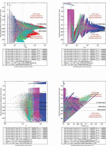
The results in Sub Figure 3(a,b,c) indicate that the observed $p_{0.05}$ values tend to converge towards the ideal 5th percentile p-value as $|{\mathcal{N}}_{\mathrm{r}\mathrm{c}}|$ or ${\hat{n}}_{\mathrm{m}\mathrm{i}\mathrm{n}}$ increases, but not when $n_{..}$ increases. The converging ${\hat{n}}_{\mathrm{m}\mathrm{i}\mathrm{n}}$ results in Sub Figure 3b are somewhat consistent with traditional criteria that the expected cell counts should be greater than some minimum value (e.g. 5, 10, or 20). The results in Sub Figure 3a also show that small $|{\mathcal{N}}_{\mathrm{r}\mathrm{c}}|$ values are undesirable, which was also expected based on the results in Sub Figure 1b and similar results in Sub Figure 2b for the Fisher-Freeman-Halton test. The lack of convergence for $n_{..}$ in Sub Figure 3c may be attributed to small $|{\mathcal{N}}_{\mathrm{r}\mathrm{c}}|$ or ${\hat{n}}_{\mathrm{m}\mathrm{i}\mathrm{n}}$ values.

The results in Sub Figure 3d show that the Pearson chi-square test p-values are outside the test p-value domain-of-validity if $min\left(p_{\mathrm{P}\mathrm{e}\mathrm{a}\mathrm{r}\mathrm{s}\mathrm{o}\mathrm{n}}\right)$ is greater than the ideal value (e.g. 0.05). Therefore 46,578 observations with $min\left(p_{\mathrm{P}\mathrm{e}\mathrm{a}\mathrm{r}\mathrm{s}\mathrm{o}\mathrm{n}}\right)>0.05$ were excluded from the envelope model quantile regression analysis.

The results in Sub Figure 3b also indicate an abrupt change near ${\hat{n}}_{\mathrm{m}\mathrm{i}\mathrm{n}}=0.05$. This change was further explored in Figure D.5, which shows that the differences between the 5th percentile Pearson and Fisher-Freeman-Halton p-values tends to peak near ${\hat{n}}_{\mathrm{m}\mathrm{i}\mathrm{n}}=0.5$. Therefore, all of the observations with ${\hat{n}}_{\mathrm{m}\mathrm{i}\mathrm{n}}\le 0.5$ were also excluded from the quantile regression analysis of the Pearson chi-square test p-values because these observations were also expected a priori to be outside the Pearson domain-of-validity and could adversely affect the overall fit to the assumed candidate model form. The estimated models for the Pearson chi-square test p-value envelope are therefore based on a fit to the remaining 10,249,393 observations, as depicted in Figure D.6. The results SubFigure D.6a more clearly shows the convergence to the ideal p-value as $|{\mathcal{N}}_{\mathrm{r}\mathrm{c}}|$ increases.

Figure 3 and D.6 also show the estimated curves for the candidate $UB$, median, and $LB$ models based on Equation (2)(2) $Q=\pi \left(g\left(p_{\mathrm{i}\mathrm{d}\mathrm{e}\mathrm{a}\mathrm{l}}\right)+sexp\left({\lambda }_0+\sum _i{\lambda }_{i}log\left(x_i\right)\right)\right)+\text{isin}$(2) . The estimated ${\lambda }_1$ and $\bar{f}$ figure-of-merit values for these and other candidate single index models are summarized in Table C.3.

3.2.2. Envelope model search results

The convergence of the observed Pearson chi-square test $p_{0.05}$ values towards the ideal 5th percentile p-value as $|{\mathcal{N}}_{\mathrm{r}\mathrm{c}}|$ or ${\hat{n}}_{\mathrm{m}\mathrm{i}\mathrm{n}}$ increases indicates the need to determine the independent effects of discreteness and approximation on the accuracy of the test. This was accomplished by considering envelope models based on Equation (1)(1) $Q=\pi \left(g\left(p_{\mathrm{i}\mathrm{d}\mathrm{e}\mathrm{a}\mathrm{l}}\right)+\sum _i\sum _j{\beta }_{i,j}{x}_i^{q_{i,j}}\right)+\text{isin}$(1) with up to four candidate indices to address different effects. The assumed candidate powers for the candidate indices based on $|{\mathcal{S}}_{\mathrm{r}\mathrm{c}}|$ or $|{\mathcal{N}}_{\mathrm{r}\mathrm{c}}|$, ${\hat{n}}_{\mathrm{m}\mathrm{i}\mathrm{n}}$, and $n_{..}$ where ${\mathrm{q}}_1=[-0.5]$ and ${\mathrm{q}}_2={\mathrm{q}}_3=[-1.0]$. The rationale for these negative powers is that the range of observed $p_{0.05}$ values is assumed to converge to the ideal 5th percentile p-value as these indices increase towards infinity, and the −0.5 and −1.0 values represent the range of ${\hat{\lambda }}_1$ results in Table C.3. The assumed candidate power for the candidate $min\left(p_{\mathrm{P}\mathrm{e}\mathrm{a}\mathrm{r}\mathrm{s}\mathrm{o}\mathrm{n}}\right)$ index was ${\mathrm{q}}_4=[1]$.

The candidate model indices and the resulting $\bar{f}$ figure-of-merit values for the Pearson chi-square test are summarized in Table C.4. The results are rank ordered from the smallest (most desirable) combined $\bar{f}$ value to the largest. These results indicate that the model with $x_1=|{\mathcal{N}}_{\mathrm{r}\mathrm{c}}|$, $x_2={\sum }_{\mathrm{m}\mathrm{i}\mathrm{n}}^{\nu }\hat{n}$, $x_3=n_{..}/\nu$, and $x_4=min\left(p_{\mathrm{P}\mathrm{e}\mathrm{a}\mathrm{r}\mathrm{s}\mathrm{o}\mathrm{n}}\right)$ had the smallest combined $\bar{f}=0.000600$. However, the estimated $LB$ and $UB$ model coefficients for the $n_{..}/\nu$ and $min\left(p_{\mathrm{P}\mathrm{e}\mathrm{a}\mathrm{r}\mathrm{s}\mathrm{o}\mathrm{n}}\right)$ terms were not statistically significant; the term based on $n_{..}$ was not consistent in the top ranked models; and the $min\left(p_{\mathrm{P}\mathrm{e}\mathrm{a}\mathrm{r}\mathrm{s}\mathrm{o}\mathrm{n}}\right)$ term did not improve the fit very much. This suggests that these three-term and four-term models may be overparameterized, which is undesirable. Dropping the terms based on $n_{..}$ and $min\left(p_{\mathrm{P}\mathrm{e}\mathrm{a}\mathrm{r}\mathrm{s}\mathrm{o}\mathrm{n}}\right)$ from the model search increases the combined $\bar{f}$ slightly from $0.000600$ to $0.000617$. The estimated model coefficients for this top ranked one-term or two-term model are listed in Table 6.

Table 6. Fifth percentile Pearson p-value envelope model fit to $|{\mathcal{N}}_{\mathrm{r}\mathrm{c}}|$ and $({\sum }_{\mathrm{m}\mathrm{i}\mathrm{n}}^{\nu }\hat{n})$

	Estimated $\beta$
Model Term	$LB$ PE $\pm$95% CI		Median PE $\pm$95% CI		$UB$ PE $\pm$95% CI
$g(p_{\mathrm{i}\mathrm{d}\mathrm{e}\mathrm{a}\mathrm{l}})$	−2.9444		−2.9444		−2.9444
$|{\mathcal{N}}_{\mathrm{r}\mathrm{c}}{|}^{-0.5}$	−2.1022$\pm$0.65233		−0.3675$\pm$1.211		1.606$\pm$1.4646
$({\sum }_{\mathrm{m}in}^{\nu }\hat{n}{)}^{-1}$	0.072932$\pm$0.53899		0.69198$\pm$0.97306		1.1235$\pm$1.2065
$\bar{f}$	0.000494		0.004432		0.000741
$N$	10,249,393

Bold font indicates the estimate is statistically significantly different from 0 at the 0.05 level of significance based on jackknife confidence intervals.

Note that the estimated $LB$ model coefficient for the ${\sum }_{\mathrm{m}\mathrm{i}\mathrm{n}}^{\nu }\hat{n}$ term in Table 6 has a small positive value that is not statistically significant. A positive value indicates that the lower bounds tends to increase for small ${\sum }_{\mathrm{m}\mathrm{i}\mathrm{n}}^{\nu }\hat{n}$ values, which is counter intuitive. If a negative sign constraint is imposed on the $LB$ model coefficients then the ${\sum }_{\mathrm{m}\mathrm{i}\mathrm{n}}^{\nu }\hat{n}$ term drops out, the $|{\mathcal{N}}_{\mathrm{r}\mathrm{c}}{|}^{-0.5}$ coefficient for the $LB$ model changes from $-2.1022\pm 0.65233$ to $-1.9942\pm 0.39061$, and $\bar{f}$ increases slightly from $0.000494$ to $0.000495$. This result appears to be consistent with the results in Figure D.6, which indicate that $|{\mathcal{N}}_{\mathrm{r}\mathrm{c}}|$ has a stronger effect on the convergence then ${\hat{n}}_{\mathrm{m}\mathrm{i}\mathrm{n}}$ for ${\hat{n}}_{\mathrm{m}\mathrm{i}\mathrm{n}}>0.5$. Dropping the ${\sum }_{\mathrm{m}\mathrm{i}\mathrm{n}}^{\nu }\hat{n}$ term from the $UB$ model is not recommended because $\bar{f}$ increases substantially from 0.000741 to 0.001110 as indicated in Table C.4.

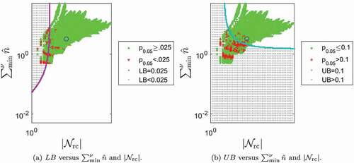
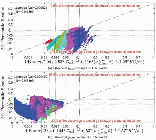
Scatter plots of the 5th percentile Pearson p-values versus the $UB$ and $LB$ models based on $|{\mathcal{N}}_{\mathrm{r}\mathrm{c}}|$ and ${\sum }_{\mathrm{m}\mathrm{i}\mathrm{n}}^{\nu }\hat{n}$ are depicted in Figure 4. The diagonal dotted lines indicate the p-values corresponding to the $UB$ and $LB$ models. Therefore, 2.5% of the observed $p_{0.05}$ values in Sub Figure 4a should be above the diagonal line, and 2.5% of the $p_{0.05}$ values in Sub Figure 4b should be below the diagonal line. The horizontal and vertical dotted lines indicate $1/2$, 1, and 2 times the ideal 5th percentile p-value for reference purposes.

Figure 4. Fifth percentile Pearson p-values versus functions of $\left|N_{rc}\right|$ and ${\mathrm{\Sigma }}_{min}^v\hat{n}$

Figure 5 depicts contours of the estimated lower and upper bound models for the 5th percentile Pearson p-value versus $|{\mathcal{N}}_{\mathrm{r}\mathrm{c}}|$ and ${\sum }_{\mathrm{m}\mathrm{i}\mathrm{n}}^{\nu }\hat{n}$. The lower bounds is depicted in Sub Figure 5a. The small $\mathrm{♢}$ symbols are a locus of points that satisfy $LB=0.025$ and the adjacent shaded region depicted by the $\circ$ symbols indicates where $LB<0.025$. The asymptotic values for the $LB=0.025$ contour are $|{\mathcal{N}}_{\mathrm{r}\mathrm{c}}|\to 8.545$ when ${\sum }_{\mathrm{m}\mathrm{i}\mathrm{n}}^{\nu }\hat{n}\to \mathrm{\infty }$, and ${\sum }_{\mathrm{m}\mathrm{i}\mathrm{n}}^{\nu }\hat{n}\to$ undefined when $|{\mathcal{N}}_{\mathrm{r}\mathrm{c}}|\to \mathrm{\infty }$ because the model coefficient is non-negative. If the ${\sum }_{\mathrm{m}\mathrm{i}\mathrm{n}}^{\nu }\hat{n}$ term is removed from this $LB$ model then the $LB=0.025$ contour is simply $|{\mathcal{N}}_{\mathrm{r}\mathrm{c}}|=$ 7.690 . The $\mathrm{\nabla }$ and $\mathrm{\Delta }$ symbols indicate the relative distributions of observed $p_{0.05}$ values $\ge 0.025$ and $<0.025$. The upper bounds is depicted in Sub Figure 5b in a similar manner. The small $\mathrm{♢}$ symbols are a locus of points that satisfy $UB=0.10$ and the shaded region indicates where $UB>0.10$. The asymptotic values for the $UB=0.10$ contour are $|{\mathcal{N}}_{\mathrm{r}\mathrm{c}}|\to 4.620$ and ${\sum }_{\mathrm{m}\mathrm{i}\mathrm{n}}^{\nu }\hat{n}\to 1.504$ when the other index goes to infinity. These results indicate that $p_{0.05}$ tends to be between 0.025 and 0.10, which is desirable, if the $|{\mathcal{N}}_{\mathrm{r}\mathrm{c}}|$ and ${\sum }_{\mathrm{m}\mathrm{i}\mathrm{n}}^{\nu }\hat{n}$ coordinate is in the unshaded region of both subfigures. The ${\sum }_{\mathrm{m}\mathrm{i}\mathrm{n}}^{\nu }\hat{n}>1.504$ criterion when $|{\mathcal{N}}_{\mathrm{r}\mathrm{c}}|\to \mathrm{\infty }$ is consistent with Cochran’s statement that “there is little disturbance to the 5% level when a single expectation is as low as $1/2$” [Cochran, 1952, p. 329].

Figure 5. Fifth percentile Pearson p-value envelope model contours

The $◯$ symbol in Figure 5 indicates the coordinates for $2\times 3$ tables with $\mathrm{r}=[39,11]$ and $\mathrm{c}=[35,9,6]$ (e.g. Table 1). This symbol is located in the unshaded region of both subfigures. This indicates the 5th percentile p-values for randomly sampled tables with these margin totals tend to be between 0.025 and 0.10, which is desirable from a test accuracy viewpoint.

The same $LB$ and $UB$ models can also be applied to more stringent limits such as 0.04 to 0.06. The value for the $LB=0.04$ contour would be $|{\mathcal{N}}_{\mathrm{r}\mathrm{c}}|=$ 72.9 if the ${\sum }_{\mathrm{m}\mathrm{i}\mathrm{n}}^{\nu }\hat{n}$ term is dropped. The asymptotic values for the $UB=0.06$ contour would be $|{\mathcal{N}}_{\mathrm{r}\mathrm{c}}|\to 69.3$ and ${\sum }_{\mathrm{m}\mathrm{i}\mathrm{n}}^{\nu }\hat{n}\to 5.83$ when the other index goes to infinity. This more stringent $UB$ criteria is within the range of the ${\hat{n}}_{\mathrm{m}\mathrm{i}\mathrm{n}}\ge$ 5 or 10 criterion recommended by others.

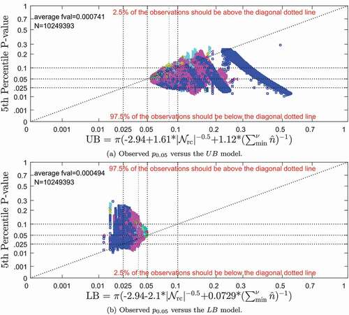
3.3. Fifth percentile Goodman-Kruskal gamma test P-values

3.3.1. Single Index trends

The results in Figure 6 compare the 5th percentile p-values from the Monte Carlo simulations of the Goodman–Kruskal Gamma test based on $AS{E}_0$ to $|{\mathcal{O}}_{\mathrm{r}\mathrm{c}}|$, ${\hat{n}}_{\mathrm{m}\mathrm{i}\mathrm{n}}$, $n_{..}$, and $min\left(p_{\mathrm{G}{\mathrm{K}}_0}\right)$ respectively. The format of this figure is also similar to Figure 2. The total number of $p_{0.05}$ observations was 24,578,997.

Figure 6. Fifth percentile Goodman-Kruskal p-values (based on ASE0) versus$\left|O_{rc}\right|$, ${\hat{n}}_{min}$,$n..$, $min\left(p_{GK0}\right)$

Like the results for the Pearson chi-square test, the results in Sub Figure 6(b,c) for the Goodman-Kruskal gamma test indicate that the observed $p_{0.05}$ values tend to converge towards the ideal 5th percentile p-value as ${\hat{n}}_{\mathrm{m}\mathrm{i}\mathrm{n}}$ increases, but not when $n_{..}$ increases. The results in Sub Figure 6a indicate that the observed $p_{0.05}$ values appear to converge to values less than the ideal 5th percentile p-value as $|{\mathcal{O}}_{\mathrm{r}\mathrm{c}}|$ increases, indicating possible liberal bias.

The results in Sub Figure 6d show that the Goodman-Kruskal gamma test p-values are outside the test p-value domain-of-validity if $min\left(p_{\mathrm{G}{\mathrm{K}}_0}\right)$ is greater than the ideal value (e.g. 0.05). Therefore 152,072 observations with $min\left(p_{\mathrm{G}{\mathrm{K}}_0}\right)>0.05$ were excluded from the envelope model quantile regression analysis.

In addition, it was observed in Figure D.4 that the differences between the 5th percentile p-values from two different versions of the Goodman-Kruskal gamma test are the largest when ${\hat{n}}_{\mathrm{m}in}$ is about 0.5. This result is similar to, but more pronounced than, the differences between the Fisher-Freeman-Halton and Pearson $p_{0.05}$ values observed in Figure D.5. Therefore, all of the observations with ${\hat{n}}_{\mathrm{m}\mathrm{i}\mathrm{n}}\le 0.5$ were excluded from the quantile regression analysis of the Goodman-Kruskal gamma test p-values because they could adversely affect the overall fit to the assumed candidate model form. The estimated models for the Goodman-Kruskal gamma test p-value envelope are therefore based on a fit to the remaining 10,143,899 observations with ${\hat{n}}_{\mathrm{m}\mathrm{i}\mathrm{n}}>0.5$, as depicted in Figure D.7. The results in SubFigure D.7a also more clearly shows convergence, but not to the ideal p-value, as $|{\mathcal{O}}_{\mathrm{r}\mathrm{c}}|$ increases.

3.3.2. Envelope model search results

Like the Pearson chi-square test, the convergence of the observed Goodman-Kruskal gamma test $p_{0.05}$ values as $|{\mathcal{O}}_{\mathrm{r}\mathrm{c}}|$ or ${\hat{n}}_{\mathrm{m}\mathrm{i}\mathrm{n}}$ increases also indicates the need to elucidate the independent effects of discreteness and approximation on the accuracy of the test. This was also accomplished by considering envelope models based on Equation (1)(1) $Q=\pi \left(g\left(p_{\mathrm{i}\mathrm{d}\mathrm{e}\mathrm{a}\mathrm{l}}\right)+\sum _i\sum _j{\beta }_{i,j}{x}_i^{q_{i,j}}\right)+\text{isin}$(1) with up to four candidate indices. The assumed candidate ${\mathrm{q}}_i$ were the same as for the Pearson chi-square test envelope models, based on similar rationale.

The candidate model indices and the resulting $\bar{f}$ figure-of-merit values for the Goodman-Kruskal gamma test are summarized in Table C.6. The results in this table are also rank ordered from the smallest (most desirable) combined $\bar{f}$ value to the largest. These results indicate that of the candidate model with $x_1=|{\mathcal{O}}_{\mathrm{r}\mathrm{c}}|$, $x_2=\nu {\sum }_{\mathrm{m}\mathrm{i}\mathrm{n}}^{\nu }\hat{n}$, $x_3=n_{..}/RC$, and $x_4=min\left(p_{\mathrm{G}{\mathrm{K}}_0}\right)$ had the smallest combined $\bar{f}=0.000537$. However, the top ranked model with only three indices fits almost as well. This model drops the $min\left(p_{\mathrm{G}\mathrm{K}}\right)$ index and the combined $\bar{f}$ value increases slightly from 0.000537 to 0.000547 . The estimated model coefficients for this envelope model are listed in (Table 7).⁹

Table 7. Fifth percentile Goodman-Kruskal ($AS{E}_0$) p-value envelope model fit to $|{\mathcal{O}}_{\mathrm{r}\mathrm{c}}|$, $(\nu {\sum }_{\mathrm{m}\mathrm{i}\mathrm{n}}^{\nu }\hat{n})$, and $(n_{..}/RC)$

	Estimated $\beta$
Model Term	$LB$ PE $\pm$95% CI	Median PE $\pm$95% CI	$UB$ PE $\pm$95% CI
$g(p_{\mathrm{i}\mathrm{d}\mathrm{e}\mathrm{a}\mathrm{l}})$	−2.9444	−2.9444	−2.9444
$|{\mathcal{O}}_{\mathrm{r}\mathrm{c}}{|}^{-0.5}$	−0.14354$\pm$0.59883	0.28106$\pm$1.5062	2.5314$\pm$2.1447
$(\nu {\sum }_{\mathrm{m}\mathrm{i}\mathrm{n}}^{\nu }\hat{n}{)}^{-1}$	−6.5337$\pm$1.347	−1.0348$\pm$2.2272	−0.11623$\pm$2.9967
$RC/n_{..}$	−1.5661$\pm$0.74461	−1.5585$\pm$0.84597	−1.2934$\pm$3.0602
$\bar{f}$	0.000470	0.003628	0.000624
$N$	10,143,899

Bold font indicates the estimate is statistically significantly different from 0 at the 0.05 level of significance based on jackknife confidence intervals.

Scatter plots of the 5th percentile Goodman-Kruskal p-values (based on $AS{E}_0$) versus the $UB$ and $LB$ models in Table 7 are depicted in Figure 7. The format and interpretation of these plots are similar to Figure 4

Figure 7. Fifth percentile Goodman-Kruskal p-values (based on ASE0) versus $\left|O_{rc}\right|$, $v{\mathrm{\Sigma }}_{min}^v\hat{n}$, and $n../RC$

Figure 7. Fifth percentile Goodman-Kruskal p-values (based on $AS{E}_0$) versus functions of $|{\mathcal{O}}_{\mathrm{r}\mathrm{c}}|$, $\nu {\sum }_{\mathrm{m}\mathrm{i}\mathrm{n}}^{\nu }\hat{n}$, and $n_{..}/RC$.

Contours of the estimated lower and upper bound models for the 5th percentile Goodman-Kruskal p-value versus $|{\mathcal{O}}_{\mathrm{r}\mathrm{c}}|$, $\nu {\sum }_{\mathrm{m}\mathrm{i}\mathrm{n}}^{\nu }\hat{n}$, and $n_{..}/RC$ are depicted in Figure D.8 in Appendix D. These plots graphically illustrate that $p_{0.05}$ tends to be between 0.025 and 0.10, which is desirable, if the $|{\mathcal{O}}_{\mathrm{r}\mathrm{c}}|$, $\nu {\sum }_{\mathrm{m}\mathrm{i}\mathrm{n}}^{\nu }\hat{n}$, and $n_{..}/RC$ coordinate is in the unshaded region of all of the subfigures. The $◯$ symbols, which represent the indices for the example in Table 1, are outside this desired (i.e. unshaded) region. This could explain the anomalous Goodman-Kruskal gamma test result listed in Table 2.

4. Limitations

The results herein are based on Monte Carlo analysis of $R\times C$ contingency tables within the simulation domain listed in Table 4. It is assumed that the results for tables with $R>C$ are equivalent to results for tables with $R<C$ due to the symmetry of the hypothesis tests. It is also assumed that the $R\times C$ tables are randomly sampled with fixed row and column margin totals. The observed 5th percentile p-value for each row and column margin total combination is based a random sample of 100,000 tables. The p-value accuracy results are limited to tables with row and column margin totals within the p-value domain-of-validity. The results for the Fisher-Freeman-Halton exact test envelope models are also limited to tables with $|{\mathcal{N}}_{\mathrm{r}\mathrm{c}}|\ge 2$; and the Pearson chi-square test and Goodman-Kruskal gamma test envelope models are limited to tables with ${\hat{n}}_{\mathrm{m}\mathrm{i}\mathrm{n}}>0.5$. The estimated envelope models are based on the assumption that all of the 5th percentile p-values for each set of fixed row and column margin totals within the simulation domain are equally weighted. The results are based on a critical test p-value of 0.05, but the methodology and results could be extended to other critical p-values.

5. Recommendations

The following criteria to determine whether or not a hypothesis test should be used for a given $R\times C$ contingency table are recommended based on the results in the previous section. These criteria comprise two parts and are based on the table dimensions and margin totals.

First, the critical p-value must be within the p-value domain-of-validity of the hypothesis test. This can be evaluated by calculating the minimum possible hypothesis test p-value using the most extreme table with the same row and column margin totals. If the minimum possible p-value is greater than or equal to the critical p-value then the test is not reliable and should not be used. It is assumed that the maximum possible p-value is always greater than the critical p-value and does not need to be evaluated.

If the p-value domain-of-validity criterion is met, then the p-value accuracy criteria is evaluated. Ideally the $\alpha$’th percentile p-value for a hypothesis test would be $\alpha$/100% if the null hypothesis is true. We propose that the lower and upper bounds for the percentile p-value corresponding to the critical p-value should be within a factor of two of the critical p-value. For example, if the critical p-value is 0.05, then the $LB$ and $UB$ for the 5th percentile p-value should be between 0.025 and 0.10.¹⁰ If not then the test p-value may be inaccurate (i.e. either too liberal or too conservative) and unreliable. This involves calculating the $LB$ and $UB$ values using Equation (1)(1) $Q=\pi \left(g\left(p_{\mathrm{i}\mathrm{d}\mathrm{e}\mathrm{a}\mathrm{l}}\right)+\sum _i\sum _j{\beta }_{i,j}{x}_i^{q_{i,j}}\right)+\text{isin}$(1) . Indices and estimated coefficients for the Fisher-Freeman-Halton exact test for tables up to $3\times 3$ and $2\times 4$ are provided in Table 5 for the 5th percentile p-value. Indices and estimated coefficients for the Pearson chi-square test and the $AS{E}_0$ version of the Goodman-Kruskal gamma test for tables up to $4\times 4$ and $2\times 5$ are provided in Tables 6 and 7 for the 5th percentile p-value, provided that ${\hat{n}}_{\mathrm{m}\mathrm{i}\mathrm{n}}>0.5$.¹¹ Example envelope model calculations are in Appendix E. R run scripts to evaluate the recommended criteria are also provided in the supplemental material (see Appendix G).

5.1. Fisher-Freeman-Halton exact test accuracy criteria

The p-value accuracy criterion for the Fisher-Freeman-Halton test with a critical p-value of 0.05 is satisfied if $|{\mathcal{N}}_{\mathrm{r}\mathrm{c}}|\ge 20.955$. The $|{\mathcal{N}}_{\mathrm{r}\mathrm{c}}|$ value can be calculated by the algorithm in Appendix B.2.

5.2. Pearson Chi-Square test accuracy criteria

The p-value accuracy criteria for the Pearson chi-square test depend on both $|{\mathcal{N}}_{\mathrm{r}\mathrm{c}}|$ and ${\sum }_{\mathrm{m}\mathrm{i}\mathrm{n}}^{\nu }\hat{n}$. This criteria can be graphically evaluated by referring to Figure 5. If the $|{\mathcal{N}}_{\mathrm{r}\mathrm{c}}|$ versus ${\sum }_{\mathrm{m}\mathrm{i}\mathrm{n}}^{\nu }\hat{n}$ coordinate is in one or both of shaded regions in Figure 5 then the test p-value may be either too liberal or too conservative. If the coordinate is in the unshaded region of both subfigures then the recommended criteria for the Pearson chi-square test are satisfied.

The p-value accuracy criteria for the Pearson chi-square test can also be numerically evaluated using Equation (1)(1) $Q=\pi \left(g\left(p_{\mathrm{i}\mathrm{d}\mathrm{e}\mathrm{a}\mathrm{l}}\right)+\sum _i\sum _j{\beta }_{i,j}{x}_i^{q_{i,j}}\right)+\text{isin}$(1) and the model coefficients in Table 6. The $LB$ and $UB$ values should be within a factor of two of the ideal value (0.05). Otherwise the test could be too liberal if $LB<0.025$ or too conservative if $UB>0.10$.

An example calculation for the 5th percentile Pearson chi-square test p-value envelope is in Table E.2. This example indicates that the 5th percentile p-value for randomly sampled $2\times 3$ tables with $\mathrm{r}=[39,11]$ and $\mathrm{c}=[35,9,6]$ is between 0.039402 and 0.083430 for 95% of the tables. This range is between 0.025 and 0.10, which is desirable from a test accuracy viewpoint.

5.3. Goodman–Kruskal Gamma test accuracy criteria

The p-value accuracy criteria for the Goodman-Kruskal gamma test depend on $|{\mathcal{O}}_{\mathrm{r}\mathrm{c}}|$, $\nu {\sum }_{\mathrm{m}\mathrm{i}\mathrm{n}}^{\nu }\hat{n}$, and $n_{..}/RC$. This criteria require the calculation of $LB$ and $UB$ to determine if the range is within a factor of two of the ideal value (e.g. 0.05). The $LB$ and $UB$ values are calculated using Equation (1)(1) $Q=\pi \left(g\left(p_{\mathrm{i}\mathrm{d}\mathrm{e}\mathrm{a}\mathrm{l}}\right)+\sum _i\sum _j{\beta }_{i,j}{x}_i^{q_{i,j}}\right)+\text{isin}$(1) and the model coefficients in Table 7. The $|{\mathcal{O}}_{\mathrm{r}\mathrm{c}}|$ value can be calculated by the algorithm in Appendix B.3.

An example calculation for the 5th percentile Goodman-Kruskal gamma test p-value envelope is in Table E.3. This example indicates that the 5th percentile p-value for randomly sampled $2\times 3$ tables with $\mathrm{r}=[39,11]$ and $\mathrm{c}=[35,9,6]$ is between 0.015660 and 0.057842 for 95% of the tables. This range is not within a factor of two of the ideal value (0.05), which is undesirable from a test accuracy viewpoint.

Therefore, these recommended criteria indicate that the example $2\times 3$ table listed in Table 1 is within the domain-of-validity of the Fisher-Freeman-Halton exact test and the Pearson chi-square test, but not within domain-of-validity of the Goodman-Kruskal gamma test. This could explain the apparently inconsistent hypothesis test results listed in Table 2.

6. Conclusions

The domain-of-validity and accuracy of the Fisher-Freeman-Halton exact, Pearson chi-square, and Goodman-Kruskal gamma tests for small $R\times C$ contingency tables were investigated. The Fisher-Freeman-Halton exact test and the Pearson chi-square test consider whether or not the frequencies in a contingency table have equal underlying proportions or independence. The Goodman-Kruskal gamma test considers whether or not a measure of association based on the frequencies in the table is statistically significant.

The investigation involved Monte Carlo simulations of randomly sampled contingency tables up to $4\times 4$ and $2\times 5$ in which the row and column variables were independent (i.e. equal underlying proportions). One hundred thousand tables were randomly sampled from each set of fixed row and column margin totals, for all margin total sets up to a pre-determined maximum table total (e.g. 200 for $2\times 2$ tables). P-values for each test were calculated for each sampled table, and the 5th percentile p-values were determined for each set of row and column margin totals.

It was observed that there were some sets of row and column margin totals for which the minimum possible p-value for a given hypothesis test was greater than likely critical p-values (e.g. 0.05). If this condition occurs than the $R\times C$ table is outside the p-value domain-of-validity of the hypothesis test and the test should not be used.

Envelope models were then estimated using quantile regressions to describe the range of the 5th percentile p-values observed in the Monte Carlo simulations. Candidate indices related to the discreteness and approximation accuracy of the p-value distributions, the total table counts, and the minimum possible p-value were considered. The indices can be calculated from $R$, $C$, and the row and column margin totals using the equations and algorithms described herein. The 2.5% and 97.5% quantiles were used to describe the lower and upper bounds of the range in the 5th percentile p-values. Data outside the p-value domain-of-validity were not used for these regressions.

The results for the Fisher-Freeman-Halton exact test indicated that this test tends to be conservative (i.e. the 5th percentile p-value tends to be greater than 0.05), and that the p-value accuracy depends on the number of possible $R\times C$ tables with unique nominal probabilities ($|{\mathcal{N}}_{\mathrm{r}\mathrm{c}}|$). The lower bounds is approximately equal to the ideal 5th percentile p-value provided that $|{\mathcal{N}}_{\mathrm{r}\mathrm{c}}|>1$. The upper bounds is within a factor of two of the ideal 5th percentile p-value if $|{\mathcal{N}}_{\mathrm{r}\mathrm{c}}|\ge 20.955$.

The results for the Pearson chi-square test indicated that this test tends to be unbiased (i.e. the median 5th percentile p-value tends to be about 0.05), and that the p-value accuracy depends on $|{\mathcal{N}}_{\mathrm{r}\mathrm{c}}|$ and the sum of the $\nu$ smallest expected cell counts (${\sum }_{\mathrm{m}\mathrm{i}\mathrm{n}}^{\nu }\hat{n}$), where $\nu$ is the number of degrees-of-freedom for the chi-square statistic. Equations and model coefficients are provided in Table 6 to estimate the range of 5th percentile chi-square test p-values based on $R$, $C$, and the row and column margin totals. The values for $|{\mathcal{N}}_{\mathrm{r}\mathrm{c}}|$ and ${\sum }_{\mathrm{m}\mathrm{i}\mathrm{n}}^{\nu }\hat{n}$ for which the lower and upper bounds for the 5th percentile p-values are within 0.025 and 0.10 are graphically depicted in Figure 5.

The results for the Goodman-Kruskal gamma test indicated that the p-value accuracy depends on the number of possible $R\times C$ tables with unique ordinal probabilities ($|{\mathcal{O}}_{\mathrm{r}\mathrm{c}}|$), $\nu {\sum }_{\mathrm{m}\mathrm{i}\mathrm{n}}^{\nu }\hat{n}$, and $n_{..}/RC$. Equations and model coefficients are provided in Table 7 to estimate the range of 5th percentile gamma test p-values based on $R$, $C$, and the row and column margin totals.

We propose that the lower and upper bounds for the percentile p-value corresponding to the critical p-value should be within a factor of two of the critical p-value. Therefore, if the critical p-value is 0.05, then the $LB$ and $UB$ for the 5th percentile p-value should be between 0.025 and 0.10. The accuracy of the 5th percentile Fisher-Freeman-Halton p-value is with this range if $|{\mathcal{N}}_{\mathrm{r}\mathrm{c}}|\ge 20.955$. Other levels of p-value accuracy can also be specified, such as between 0.04 and 0.06. The accuracy criteria for the Pearson chi-square test depends on $|{\mathcal{N}}_{\mathrm{r}\mathrm{c}}|$ and ${\sum }_{\mathrm{m}\mathrm{i}\mathrm{n}}^{\nu }\hat{n}$, and the Goodman-Kruskal gamma test depends on $|{\mathcal{O}}_{\mathrm{r}\mathrm{c}}|$, $\nu {\sum }_{\mathrm{m}\mathrm{i}\mathrm{n}}^{\nu }\hat{n}$, and $n_{..}/RC$.

An example application of the proposed criteria to a $2\times 3$ contingency table was also given. These criteria indicated that the example $2\times 3$ table is within the domain-of-validity of two of the three hypothesis tests investigated.

The criteria presented herein is specific to the 0.05 critical p-value. Criteria specific to other critical p-values (e.g. 0.01) or other hypothesis tests could also be determined using the methods described herein.

Disclosure statement

No potential conflict of interest was reported by the authors.

Supplementary Material

Supplemental data for this article can be accessed here.

Additional information

Funding

This work was supported by American Honda Motor Co., Inc. [NA];

Notes on contributors

R. M. Van Auken

R. M. Van Auken and S. A. Kebschull have been involved in various multi-disciplinary applied research projects primarily for the ground vehicle industry. Research activities involved modeling, simulation, testing, and analysis of human-vehicle-environmental systems; including vehicle dynamics, manual control, biomechanics, accident data analysis, and risk/benefit analysis. They have also been involved in regulation, testing and standards development. Some of these activities involved analysis of contingency tables using hypothesis tests such as the Fisher exact, Pearson chi-square, and Goodman-Kruskal gamma tests. The results of the research reported herein provided useful insight and understanding for suitability and interpretation of these hypothesis test results.

Notes

1. The results in this paper are specific to a critical p-value of 0.05 because this value is widely used. See [Box, Hunter, and Hunter, 1978, p. 109] and (Wasserstein & Lazar, 2016). Other critical p-values such as 0.01 have also been used. The methods used herein could be extended to these other critical p-values in the future.

2. Norušis states `[i]f you reject the null hypothesis that two variables are independent, you may want to describe the nature and strength of the relationship between the two variables’ [Norušis, 2008, p. 172]. This suggests that association is only meaningful if the null hypothesis for independence can be rejected.

3. In our notation $k=RC$ and $n=n_{..}$.

4. See footnote 1.

5. This condition can occur in $2\times 2$ tables even for large $n_{..}$ if one of the row margin totals is equal to 1 and the column margin totals are equal. For example, if $\mathrm{r}=[1,199]$ and $\mathrm{c}=[100,100]$.

6. Many of the 14,154,495 symbols in Figure 2 mask other symbols due to the symbol size and drawing order. The symbols were drawn in random order in order to depict the relative distribution of the table dimensions. The absolute distribution of the observed p-values is not depicted because of masking.

7. The criteria for a desirable range of $p_{0.05}$ values is arbitrary but directly relates to test p-value accuracy. Cochran [Cochran, 1952, pp. 328–329] suggested a range between 0.04 and 0.06 for a critical p-value of 0.05. Cochran acknowledged that these `limits are, of course, arbitrary; some would be content with less conservative limits.’ We are using a range of 0.025 to 0.10, which corresponds to a relative factor of 2, and is less conservative then Cochran’s suggested limits.

8. If we use the estimated alternative model coefficients in Table D.2 then the 95% interval for $p_{0.05}$ the Fisher-Freeman-Halton test would exceed 0.10 if $|{\mathcal{N}}_{\mathrm{r}\mathrm{c}}|<21.738$ and $min\left(p_{\mathrm{F}\mathrm{i}\mathrm{s}\mathrm{h}\mathrm{e}\mathrm{r}}\right)=0$.

9. The envelope model search results in Tables C.5 and C.6 indicate that models based on $|{\mathcal{S}}_{\mathrm{r}\mathrm{c}}|$ tend to fit the distribution of 5th percentile Goodman-Kruskal gamma test p-values almost as well as $|{\mathcal{O}}_{\mathrm{r}\mathrm{c}}|$. The $|{\mathcal{S}}_{\mathrm{r}\mathrm{c}}|$ index requires less effort to calculate than $|{\mathcal{O}}_{\mathrm{r}\mathrm{c}}|$, which is desirable. Estimated coefficients for an alternative Goodman-Kruskal gamma test envelope model based on $|{\mathcal{S}}_{\mathrm{r}\mathrm{c}}|$ are listed in Table D.3 in Appendix D.5.

10. Cochran [Cochran, 1952, pp.328–329] suggested a range between 0.04 and 0.06 for a critical p-value of 0.05, and a range between 0.007 and 0.015 for a critical p-value of 0.01. Cochran acknowledged that these `limits are, of course, arbitrary; some would be content with less conservative limits.’ Our proposed limits are also arbitrary and less conservative than Cochran’s limits.

11. We can reasonably assume that the Pearson chi-square and Goodman-Kruskal gamma tests are not valid if ${\hat{n}}_{\mathrm{m}\mathrm{i}\mathrm{n}}\le 0.5$ based on traditional criteria and extrapolation of the envelope models.

References

- Agresti, A. (1996). An introduction to categorical data analysis. John Wiley & Sons, Inc.
- Agresti, A. (2002). Categorical data analysis. John Wiley & Sons, Inc. http://mathdept.iut.ac.ir/sites/mathdept.iut.ac.ir/files/AGRESTI.PDF
- Box, G. E., Hunter, W. G., & Hunter, J. S. (1978). Statistics for experimenters, an introduction to design, data analysis, and model building. John Wiley & Sons.
- Brown, M. B., & Benedetti, J. K. (1977). Sampling behavior of tests for correlation in two-way contingency tables. Journal of the American Statistical Association, 72(358), 309–20. DOI: https://doi.org/10.1080/01621459.1977.10480995
- Cardillo, G. (2007a). Myfisher23: A very compact routine for fisher’s exact test on 2x3 matrix (version 2.0, updated 2018-05-04) [The mathworks, inc.]. https://www.mathworks.com/matlabcentral/fileexchange/15399-myfisher23
- Cardillo, G. (2007b). Myfisher24: A very compact routine for fisher’s exact test on 2x4 matrix (version 2.0, updated 2018-04-06) [The mathworks, inc.]. https://www.mathworks.com/matlabcentral/fileexchange/19842-myfisher24
- Cardillo, G. (2007c). Myfisher33: A very compact routine for fisher’s exact test on 3x3 matrix (version 2.0, updated 2018-04-06) [The mathworks, inc.]. https://www.mathworks.com/matlabcentral/fileexchange/15482-myfisher33
- Cochran, W. G. (1952). The χ2 test of goodness of fit. The Annals of Mathematical Statistics, 23(3), 315–345. https://doi.org/https://doi.org/10.1214/aoms/1177729380
- Cochran, W. G. (1954). Some methods for strengthening the common χ2 tests. Biometrics, 10(4), 417–451. https://doi.org/https://doi.org/10.2307/3001616
- Craddock, J. M., & Flood, C. R. (1970). The distribution of the χ2 statistic in small contingency tables. Journal of the Royal Statistical Society. Series C, Applied Statistics, 19(2), 173–181. https://rss.onlinelibrary.wiley.com/doi/abs/ https://doi.org/10.2307/2346547
- Cramer, H. (1946). Mathematical Methods of Statistics. Princeton University Press, Princeton.
- Diaconis, P., & Gangolli, A. (1994). Rectangular arrays with fixed margins (pp. 452). Department of Statistics, Stanford University. https://statistics.stanford.edu/sites/g/files/sbiybj6031/f/EFS%20NSF%20452.pdf
- Ehwerhemuepha, L., Sok, H., & Rakovski, C. (2019). A more powerful unconditional exact test of homogeneity for 2 × c contingency table analysis. Journal of Applied Statistics, 46(14), 2572–2582. https://doi.org/https://doi.org/10.1080/02664763.2019.1601689
- Ekstrøm CT. (2020). MESS: Miscellaneous esoteric statistical scripts. R package version 0.5.7. https://CRAN.R-project.org/package=MESS
- Electronics Reliability Subcommittee. (1987). Automotive electronics reliability handbook. Society of Automotive Engineers, Inc.
- Fisher, R. A. (1934). Statistical methods for research workers (5th ed.). Oliver and Boyd.
- Fleiss, J. L. (1981). Statistical methods for rates and proportions (2nd ed.). John Wiley & Sons.
- Freeman, G., & Halton, J. (1951). Note on an exact treatment of contingency, goodness of fit and other problems of significance. Biometrika, 38(1–2), 141–149. https://doi.org/https://doi.org/10.1093/biomet/38.1-2.141
- Gail, M., & Mantel, N. (1977). Counting the number of contingency tables with fixed margins. Journal of the American Statistical Association, 72(360a), 859–862. DOI: https://doi.org/10.1080/01621459.1977.10479971
- Göktaş, A., & İşçi, O. (2011). A comparison of the most commonly used measures of association for doubly ordered square contingency tables via simulation. Metodološki Zvezki, 8(1), 17–37. http://mrvar.fdv.uni-lj.si/pub/mz/mz8.1/goktas.pdf
- Good, I. J., Gover, T. N., and Michell, G. (1970). Exact distributions for X2 and the likelihood ratio statistic for the equiprobable multinomial distribution. Journal of the American Statistical Association, 65(1), 267.
- Goodman, L. A., & Kruskal, W. H. (1979). Measures of association for cross classifications. Springer-Verlag.
- Grinsted, A. (2008). quantreg: Quantile regression with bootstrapping confidence intervals (version 1.3.0.0) [The mathworks, inc.]. https://www.mathworks.com/matlabcentral/fileexchange/32115-quantreg-x-y-tau-order-nboot
- Kahane, C. (2012). Relationships between fatality risk, mass, and footprint in model year 2000–2007 passenger cars and LTVs - final report. National Highway Traffic Safety Administration. DOT HS 811 665 https://www.regulations.gov/document/NHTSA-2010-0152-0040
- Kendal, M. G. (1952). The Advanced Theory of Statistics (5th Ed. Vol. 1). Griffin, London
- Koehler, K. J., & Larntz, K. (1980). An empirical investigation of goodness-of-fit statistics for sparse multinomials. Journal of the American Statistical Association, 75(370), 336–344. https://doi.org/https://doi.org/10.1080/01621459.1980.10477473
- Kroese, D. P., & Chan, J. C. C. (2014). Statistical modeling and computation. Springer.
- MathWorks. (2016). Statistics and machine learning toolboxTM user’s guide.
- Mehta, C. R., & Patel, N. R. (1986). Algorithm 643: Fexact: A fortran subroutine for fisher’s exact test on unordered r × c contingency tables. ACM Transactions on Mathematical Software (TOMS), 12(2), 154–161. https://doi.org/https://doi.org/10.1145/6497.214326
- Norušis, M. J. (2008). SPSS 16.0 statistical procedures companion. Prentice Hall, Inc.
- Ott, R. L., Larson, R., Rexroat, C., and Mendenhall, W. (1992). Statistics, a tool for the social sciences. Duxbury Press.
- R Core Team. (2017). R: A language and environment for statistical computing. R Foundation for Statistical Computing. https://www.R-project.org/
- Rosenthal, I. (1966). Distribution of the sample version of the measure of association, gamma. Journal of the American Statistical Association, 61(314):440–453. https://doi.org/https://doi.org/10.1080/01621459.1966.10480880
- SAS. (2013). Base SAS® 9.4 procedures guide: Statistical procedures, second edition. SAS Institute Inc. http://support.sas.com/documentation/cdl/en/procstat/66703/PDF/default/procstat.pdf
- SPSS. (2009). PASW® statistics 18 command syntax reference.
- SPSS. (2010). IBM SPSS statistics 19 algorithms. Available from: http://www.sussex.ac.uk/its/pdfs/SPSS_Algorithms_19.pdf
- Tate, M. W., & Hyer, L. A. (1973). Inaccuracy of the x2 test of goodness of fit when expected frequencies are small. Journal of the American Statistical Association, 68(344), 836–841. DOI: https://doi.org/10.1080/01621459.1973.10481433
- Wasserstein, R. L., & Lazar, N. A. (2016). The asa’s statement on p-values: Context, process, and purpose. The American Statistician, 70(2), 440–453. https://doi.org/https://doi.org/10.1080/00031305.2016.1154108