Dealing with covariate measurement error in a clustered cross-sectional survey

Abstract

Many surveys are often complex cross-sectional studies that involve clustered data. Such surveys can have the additional complexity of the measurement error problem. Ignoring the measurement error problem and the clustering aspect may lead to incorrect inferences and conclusions. The purpose of this study was to demonstrate the application of regression calibration to correct for covariate measurement error in a clustered cross-sectional survey in a generalized estimating equations (GEE) framework. Methods that ignore both covariate measurement error and within-cluster correlation structure are compared to the proposed regression calibration-GEE method. The study found that clustering does not affect the association estimates adjusted for measurement error using regression calibration. However, the standard errors of the coefficient estimates are overestimated or underestimated in methods that ignore the within-cluster dependency despite adjusting for measurement error. Specifically, for clusters of size 10 and under unstructured and exchangeable correlation structure, the standard error was about 10.3% higher and 13.6% lower, respectively, in the method that ignores the within-cluster dependency than in the proposed method. From the findings of this study, we conclude that it is important to adjust for covariate measurement error in clustered data, while accounting for the within-cluster correlation.

Keywords:

• Clustered survey
• covariate measurement error
• regression calibration
• generalized estimating equations

PUBLIC INTEREST STATEMENT

Cross-sectional surveys are widely used to collect data from the population of interest. Features such as stratification and sampling weights form a critical part in designing surveys. Data collected from surveys are prone to measurement error. Measurement error in covariates/exposures is often ignored in statistical analyses, despite its adverse effects on the results. This study provides insights on how to model the association between an outcome and a covariate, while adjusting for measurement error in the covariate and addressing the within-cluster dependencies in clustered cross-sectional data. We hope that the findings of this study will positively impact how the public handles data from cross-sectional surveys. This will help present correct inferences from statistical analyses of survey data, advance science faster, and benefit society.

1. Introduction

Many surveys are often complex in design and cross-sectional in nature. These surveys make use of data collection tools that are prone to measurement error, for instance, self-reported questionnaires. Measurement error (ME) in exposures (or covariates) biases the association between the covariate and an outcome. The bias can be in any direction depending on the error structure (Agogo, 2017; Fosgate, 2006; Fuller, 2009; Hill & Kleinbaum, 2014; Stefanski, 1985). Study designs range from simple designs to complicated ones. In many cross-sectional surveys with complex study design features, data within clusters are usually correlated (Akter et al., 2018; Hanley et al., 2003; Liang & Zeger, 1993; Neuhaus et al., 1991; Santos et al., 2008). Analysis of such data using standard methods that ignore covariate ME and clustering, may lead to invalid inference and conclusions. Regression calibration (RC) is a popular technique for adjusting for ME in a continuous covariate. Regression calibration is the conditional expectation of the true covariate, given the measured covariate and a vector of error-free covariates (Agogo et al., 2014; Carroll et al., 2006; Carroll & Stefanski, 1990; Freedman et al., 2008; Gleser, 1990). In a clustered survey, generalized estimating equations (GEE) approach is commonly used to account for the within-cluster dependencies, while estimating the association parameter of interest (Hanley et al., 2003; Liang & Zeger, 1986; Zeger & Liang, 1986).

Currently, there is limited research focusing on correcting for covariate ME, while accounting for survey design simultaneously in cross-sectional surveys. In this work, we demonstrated how to apply RC in a GEE context to correct for covariate ME while accounting for within-cluster correlation. We re-emphasize the need to correct for ME in a covariate and simultaneously allow for correlation structure in clustered data.

The other sections of this paper are organized as follows: In section 2, we present the methods and materials for this study. Specifically, in section 2, we review the RC method and GEE approach, describe the simulation design and provide a real-data example. Simulation and real data results are presented in section 3. Section 4 provides a discussion and concluding remarks.

2. Methods and materials

2.1. Regression calibration method

Usually, in epidemiological studies, it is impossible to observe the true covariate of interest, $X$. Instead, we observe a mismeasured covariate, $Q$. Regression calibration was first proposed by Carroll and Stefanski (1990), and Gleser (1990) as a method for correcting ME in the covariates. Regression calibration involves approximation of the conditional expectation of the true covariate given the mismeasured covariate and a vector of error-free covariates (Freedman et al., 2008; Guolo, 2008; Küchenhoff & Carroll, 1997). The basic idea of RC is to replace $X$, which is unobservable, with an estimate ${\hat{Q}}_{calib}$, a function of the error-prone covariate $Q$ and a vector of error-free covariates $Z$. Regression calibration is applicable under the assumptions that: (i) the measurement error in the observed covariate $Q$ is non-differential with respect to $X,$ and a vector of error-free covariates. Non-differential error occurs when the measured covariate contains no extra information about the outcome other than what is contained in true covariate (Carroll et al., 2006), and (ii) the measurement error in the unbiased measurement, say, $R$ of the true covariate $X$ is uncorrelated with the measurement error in the observed covariate $Q$ and with the true covariate, $X$. Noteworthy, $R$ is a reference measurement from the calibration study.

Regression calibration is implemented in two main steps:

Step 1. Estimating the calibration function. This involves estimating the conditional expectation of $X$ given $Q$ and $Z$, denoted by

(1) $E[X|Q,Z]={\hat{Q}}_{calib},$(1)

where ${\hat{Q}}_{calib}$ is the calibrated version of $Q$. In the calibration function in equation (1) above, the unobservable true covariate $X$ is replaced with $R$, which can be obtained from a validation, replication or instrumental data. Therefore, equation (1)(1) $E[X|Q,Z]={\hat{Q}}_{calib},$(1) can be re-expressed as

(2) $E[R|Q,Z]={\hat{Q}}_{calib}.$(2)

Step 2. Using ${\hat{Q}}_{calib}$ instead of $Q$ in the standard analysis to obtain the parameter estimate that quantifies the association between the outcome and the covariate of interest given the error-free covariates.

2.2. The GEE approach

Zeger and Liang (1986) proposed the GEE to extend generalized linear models (GLMs) to analyzing correlated observations. The GEE approach requires the specification of the first two moments (mean and variance) of responses from the same cluster and a working correlation rather than the full specification of the joint distribution (Akter, Sarker, & Rahman, 2018). The GEE yields asymptotically unbiased regression coefficient estimates regardless of the specified correlation structure. The GEE estimates have marginal population-averaged interpretation.

Assume that a population of size $N$ is divided into $K$ non-overlapping clusters of sizes $n_i$ ($i=1,2,\dots ,K$) such that $\sum _i^K{n}_i=N$. Let $Y_{ij}$, $j=1,2,\dots ,n_i$ be the $j^{th}$ response from the $i^{th}$ cluster and $X_{ij}=\left\{x_{ij1},\dots ,x_{ijp}\right\}$ be a vector of the corresponding $p$ covariates. Using the GLM framework, the marginal expectation $E(Y_i|X_i)={\mu }_i=({\mu }_{i1},{\mu }_{i2}\dots ,{\mu }_{i{n}_i}{)}^{\mathrm{\top }}$ can be modeled as $\varphi \left({\mu }_i\right)=X_i\beta$, where ${\beta }^{\mathrm{\top }}=\left({\beta }_0,{\beta }_1,\dots ,{\beta }_p\right)$ is a $p$-dimensional vector of regression coefficients to be estimated, $X_i$ is a matrix whose first column is a vector of 1’s corresponding to the intercept terms and $\varphi \left(.\right)$ is the appropriate link function. For a binary response variable a logit link can be used such that the mean model can be expressed as

(3) $E(Y_{ij}|X_{ij})={\mu }_{ij}=\frac{exp\left(X_i\beta \right)}{1+exp\left(X_i\beta \right)}.$(3)

We denote the working covariance matrix by $V_i=A_i^{1/2}{\rho }_i\left(\alpha \right)A_i^{1/2}$, where $A_i$ is a diagonal matrix with a known variance function $v\left({\mu }_{ij}\right)$ and ${\rho }_i\left(\alpha \right)$ is the corresponding working correlation matrix, which depends on some vector of parameters $\alpha$ which is generally unknown. Assuming that the structure of ${\rho }_i\left(\alpha \right)$ is known, the regression parameters $\beta$ can be estimated by solving the GEE,

(4) $U\left(\beta ,\alpha \right)=\sum _{i=1}^K{D}_i^T{V}_i^{-1}\left(y_i-{\mu }_i\right)=0$(4)

where $D_i=\mathrm{\partial }{\mu }_i/\mathrm{\partial }\beta$

The four commonly used correlation structures include the exchangeable, independence, auto-regressive (AR) and unstructured structures. In the exchangeable structure, it is assumed that any two observations within a cluster are equally correlated with correlation $\rho$ (fixed) but observations between clusters are assumed to be uncorrelated. For the $i^{th}$ cluster with size $n_i$ the exchangeable (or compound symmetry) correlation matrix can be expressed as follows:

(5) ${\rho }_i\left(\alpha \right)=\left(\begin{array}{ccccc}1& {\rho }_{12}& {\rho }_{13}& \dots & {\rho }_{1n_i}\\ {\rho }_{21}& 1& {\rho }_{23}& \dots & {\rho }_{2n_i}\\ ⋮& ⋮& \ddots & \hspace{0.17em}& ⋮\\ {\rho }_{n_{i}1}& {\rho }_{n_{i}2}& {\rho }_{n_{i}3}& \dots & 1\end{array}\right)=\left(\begin{array}{ccccc}1& \rho & \rho & \dots & \rho \\ \rho & 1& \rho & \dots & \rho \\ ⋮& ⋮& \ddots & \hspace{0.17em}& ⋮\\ \rho & \rho & \rho & \dots & 1\end{array}\right).$(5)

Horton and Lipsitz (1999) proposed the exchangeable structure as the appropriate correlation structure for handling data from a complex clustered design, where observations from the same cluster are not ordered chronologically such as in the case of longitudinal data.

Under the independent (or scaled identity) correlation structure, it is assumed that there is no correlation between observations hence, no need for GEE. The independent working correlation matrix for the $i^{th}$ cluster can be expressed as follows:

(6) ${\rho }_i\left(\alpha \right)=\left(\begin{array}{ccccc}1& {\rho }_{12}& {\rho }_{13}& \dots & {\rho }_{1n_i}\\ {\rho }_{21}& 1& {\rho }_{23}& \dots & {\rho }_{2n_i}\\ ⋮& ⋮& \ddots & \hspace{0.17em}& ⋮\\ {\rho }_{n_{i}1}& {\rho }_{n_{i}2}& {\rho }_{n_{i}3}& \dots & 1\end{array}\right)=\left(\begin{array}{ccccc}1& 0& 0& \dots & 0\\ 0& 1& 0& \dots & 0\\ ⋮& ⋮& \ddots & \hspace{0.17em}& ⋮\\ 0& 0& 0& \dots & 1\end{array}\right).$(6)

In the AR correlation structure which is more appropriate for observations made over time from the same unit, repeated observations that are close together in time are strongly correlated, and the correlation becomes weaker and weaker as repeated observations get further in time. The correlation between, say the $a^{th}$ and $b^{th}$ observations in cluster $i$ is given by ${\rho }_i\left(\alpha \right)={\rho }^{\left|a-b\right|}$, where $0\le \rho \le 1$, as shown in the AR(1) correlation matrix below:

(7) ${\rho }_i\left(\alpha \right)=\left(\begin{array}{ccccc}1& {\rho }_{12}& {\rho }_{13}& \dots & {\rho }_{1n_i}\\ {\rho }_{21}& 1& {\rho }_{23}& \dots & {\rho }_{2n_i}\\ ⋮& ⋮& \ddots & \hspace{0.17em}& ⋮\\ {\rho }_{n_{i}1}& {\rho }_{n_{i}2}& {\rho }_{n_{i}3}& \dots & 1\end{array}\right)=\left(\begin{array}{ccccc}1& \rho & {\rho }^2& \dots & {\rho }^{\left|1-n_i\right|}\\ \rho & 1& \rho & \dots & {\rho }^{\left|2-n_i\right|}\\ ⋮& ⋮& \ddots & \hspace{0.17em}& ⋮\\ {\rho }^{\left|n_i-1\right|}& {\rho }^{\left|n_i-2\right|}& {\rho }^{\left|n_i-3\right|}& \dots & 1\end{array}\right).$(7)

In the unstructured correlation structure, no constraints are put, and the correlation between different observations in a cluster can be different. Though this correlation structure is flexible, fitting such a correlation structure becomes computationally costly, as the number of parameters to be estimated increases with an increase in the number of observations in a cluster.

2.2.1. GEE procedure

Zeger and Liang (1986) proposed an iterative procedure for obtaining the GEE estimates $\hat{\beta }$ of $\beta$ under exchangeable correlation structure. The first step involves choosing the initial estimate ${\beta }^0$ of $\beta$, obtained by fitting a GLM considering the independence working correlation. In the second step, we set $\hat{\beta }={\beta }^0$ and calculate moment estimate $\hat{\alpha }$ of $\alpha$, for instance, for exchangeable working correlation matrix $\rho \left(\alpha \right)$ is calculated as

(8) $\hat{\alpha }=\frac{1}{K}\sum _{i=1}^K\frac{1}{n_i\left(n_i-1\right)}\sum _{j\ne k}^{n_i}{s}_{ij}^{\ast }{s}_{ik}^{\ast }$(8)

where $s_{ij}^{\ast }=\frac{y_{ij}-{\mu }_{ij}}{\sqrt{v\left({\mu }_{ij}\right)}}$

In the third step, the working correlation matrix $\rho \left(\hat{\alpha }\right)$ obtained in the second step is used to update the current estimate ${\hat{\beta }}^t$ using the Newton–Raphson method as

(9) ${\hat{\beta }}^{t+1}={\hat{\beta }}^t+{\left[I\left(\beta ,\alpha \right)\right]}^{-1}{|}_{\beta ={\hat{\beta }}^t}U\left(\beta ,\alpha \right){|}_{\beta ={\hat{\beta }}^t}.$(9)

Steps two and three are repeated until convergence to obtain $\hat{\beta }$ of $\beta$.

The standard error (SE) of the GEE estimate is commonly calculated using the sandwich-based robust method. This is because the sandwich-based robust estimator is consistent and asymptotically unbiased, even under the mis-specification of the working correlation structure. The variance of $\hat{\beta }$, $\mathrm{v}\mathrm{a}\mathrm{r}\left(\hat{\beta }\right)$ is obtained by substituting the estimate of $\beta$ at each iteration, and updating the following equation for the final estimate:

(10) $\mathrm{v}\mathrm{a}\mathrm{r}\left(\hat{\beta }\right)={\left(\sum _{i=1}^N{D}_i^T{V}_i^{-1}{D}_i\right)}^{-1}\left(\sum _{i=1}^N{D}_i^T{V}_i^{-1}cov\left(Y_i\right)V_i^{-1}{D}_i\right){\left(\sum _{i=1}^N{D}_i^T{V}_i^{-1}{D}_i\right)}^{-1},$(10)

where $\mathrm{c}\mathrm{o}\mathrm{v}\left(Y_i\right)=E\left(Y_i-{\mu }_i\right)(Y_i-{\mu }_i{)}^{\mathrm{\top }}$

2.3. Monte Carlo simulations

In this study, we first use Monte Carlo simulations to show the application of RC in GEE for analyzing clustered data when the covariate is subject to ME. The simulations were conducted in R software. This section provides details of the simulation design, a description of the methods used and how the methods are evaluated.

2.3.1. Simulation design

For simplicity and without loss of generality, we focus on the following binary logit model with two regressors, one of which is subject to additive ME

(11) $\mathrm{l}\mathrm{o}\mathrm{g}\mathrm{i}\mathrm{t}\left[P\left(Y_{ij}=1\right)\right]=0.2X_{ij1}+0.8X_{ij2},$(11)

(12) $Q_{ij}=X_{ij1}+U_{ij},$(12)

where $X_1\sim N\left(5,4\right)$, $X_2$ is binary covariate (assumed to be error-free), $Q$ is the mis-measured version of $X_1$. The additive error $U$ is assumed to follow a normal distribution with mean 0 and variance ${\sigma }_U^2=25$. Noteworthy, the binary outcome $Y$ is generated based on $X_1$, $X_2,$ and a pre-defined working correlation structure using the rbin function in SimCorMultRes package (Touloumis, 2016).

The unbiased version, $R$, of $X_1$ is simulated such that it contains a small additive ME, $u$,

(13) $R_{ij}=X_{ij1}+u_{ij},$(13)

where $u\sim N\left(0,0.01\right)$

We generate a total of 100 clusters with cluster sizes, $n_i\in \left\{5,10,30,90,200\right\},$ assuming the commonly used correlation structures described in section 2.2. For illustrative purposes, the following $n_i\times n_i$ working correlation matrices are used in the simulation of the clustered observations:

1. For exchangeable correlation structure, we use a working correlation matrix of the form:

(14) ${\rho }_i\left(\alpha \right)=\left(\begin{array}{ccccc}1& 0.925& 0.925& \dots & 0.925\\ 0.925& 1& 0.925& \dots & 0.925\\ ⋮& ⋮& \ddots & \hspace{0.17em}& ⋮\\ 0.925& 0.925& 0.925& \dots & 1\end{array}\right).$(14)

2. AR(1) working correlation matrix is generated as

(15) ${\rho }_i\left(\alpha \right)=\left(\begin{array}{ccccc}1& 0.925& {0.925}^2& \dots & {0.925}^{\left|1-n_i\right|}\\ 0.925& 1& 0.925& \dots & {0.925}^{\left|2-n_i\right|}\\ ⋮& ⋮& \ddots & \hspace{0.17em}& ⋮\\ {0.925}^{\left|n_i-1\right|}& {0.925}^{\left|n_i-2\right|}& {0.925}^{\left|n_i-3\right|}& \dots & 1\end{array}\right),$(15)

3. For unstructured working correlation, we first generate a positive definite covariance matrix, and then convert it to a correlation matrix. This is implemented in the clusterGeneration package (Qiu et al., 2015).

4. For the independence correlation structure, we model the simulated data using GLM.

Survey weights form a key feature of complex-clustered surveys and are used to ensure that statistics calculated from data are more representative of the population of interest. To incorporate this feature, the binary covariate $X_2$ is simulated such that it contains two possible values, that is, Male and Female, with probabilities 0.6 and 0.4, respectively. To account for the simulation of the values of $X_2$ with unequal probabilities, we use the rake function in the survey package (Lumley & Lumley, 2007)  to create weights for the simulated clustered data.

2.3.2. Calibration and methods description

The calibrated version of the observable mis-measured version of $X_1$, ${\hat{Q}}_{calib}$, is the predicted value obtained in the linear regression of $R$ on $Q$, and the error-free covariate, $X_2$. Thus the calibrated exposure variable of interest is given by

(16) ${\hat{Q}}_{ijcalib}=E[R_{ij}|Q_{ij},X_{ij2}].$(16)

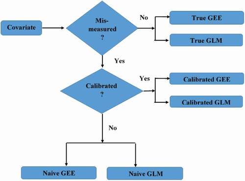
We compare the estimates of the association between the outcome and the covariate of interest obtained from the following described methods:

M1 True GEE: This method relates the outcome ($Y$) and true simulated covariate ($X_1$) and an error-free covariate ($X_2$), taking into consideration the within-cluster correlation structure.

M2 Naive GEE: In this method, we modeled the association between $Y$ and ($Q$, $X_2$), taking into consideration the within-cluster correlation structure.

M3 Calibrated GEE: A method taking into consideration the correlation structure of observations within a cluster and relating $Y$ and ($Q_{calib}$, $X_2$).

M4 True GLM: In this method, we modeled the association between $Y$ and ($X_1$, $X_2$) without taking into consideration the within-cluster correlation.

M5 Naive GLM: A method that ignores both the covariate ME and within-cluster dependencies.

M6 Calibrated GLM: This method related $Y$ and ($Q_{calib}$, $X_2$) ignoring the within-cluster dependencies.

The methods are summarized in the flow-chart diagram shown in Figure 1

Figure 1. Flow-chart diagram for the methods to be compared

2.3.3. Model evaluation

Our interest is in the coefficient estimate ${\hat{\beta }}_1$ of the parameter ${\beta }_1=0.2$, which quantifies the association between $Y$ and $X_1$. Models comparison is based on the following:

1. Relative bias in ${\hat{\beta }}_1$: Rel.bias (${\hat{\beta }}_1$) =$\frac{\mathrm{b}\mathrm{i}\mathrm{a}\mathrm{s}\left({\hat{\beta }}_1\right)}{{\beta }_1}$,

2. Empirical standard error of ${\hat{\beta }}_1$: SE (${\hat{\beta }}_1$) =$\sqrt{\frac{1}{M-1}\sum _M^{c=1}{({\hat{\beta }}_{1,c}-{\overline{\stackrel{ˆ}{\beta }}}_1)}^2}$,

3. Mean squared error of ${\hat{\beta }}_1$: MSE$\left({\hat{\beta }}_1\right)$=$\left[\mathrm{S}\mathrm{E}\left({\hat{\beta }}_1\right){]}^2+\right[\mathrm{b}\mathrm{i}\mathrm{a}\mathrm{s}\left({\hat{\beta }}_1\right){]}^2$, where ${\overline{\stackrel{ˆ}{\beta }}}_1=\frac{1}{M}\sum _M^{c=1}\left({\hat{\beta }}_{1,c}\right)$, $\mathrm{b}\mathrm{i}\mathrm{a}\mathrm{s}\left({\hat{\beta }}_1\right)={\overline{\stackrel{ˆ}{\beta }}}_1-{\beta }_1$ and ${\hat{\beta }}_{1,c}$ is the parameter estimate from the $c^{th}$ simulated data set (Burton et al., 2006).

We compared the results obtained by using the methods described in section 2.3.2, under correctly specified within-cluster correlation structure and different cluster sizes ($n_i$). We also compared the results from the different methods when the within-cluster correlation structure is mis-specified. The simulations were repeated 500 times. A random seed was used to ensure the reproducibility of the results. We provide the mean coefficient estimates and Monte Carlo standard errors in the supplemental data for this article.

2.4. Application to real data

In this study, we illustrate the use of RC to correct for covariate ME in real clustered cross-sectional data. Specifically, we used a subset data of cigarette smokers extracted from the South African National Health and Nutrition examination survey 2011–2012 (SANHANES-1). The survey applied a stratified cluster sampling approach (Human Sciences Research Council, 2017). Enumeration areas (EAs) were the primary sampling units. The selection of EAs was stratified by province. Responses from the same EA are likely to be correlated in this survey, since they share the same cluster information. We focused on modeling the association between coughing status and smoking. In the study, smoking was quantified using the self-reported average number of cigarettes smoked per week. In addition to the average number of cigarettes smoked per week, some smokers reported the number of cigarettes smoked daily. The self-reported number of cigarettes smoked weekly is prone to ME, and therefore using such in modeling the association between coughing and smoking, yields biased estimates of the association.

We first adjusted for ME in the average number of cigarettes smoked per week before modeling the association between coughing and smoking. In this study, the number of cigarettes smoked daily was used to calibrate those smoked weekly in the following RC setting:

(17) $E[R_{ij}|Q_{ij},Z_{ij}]={\hat{Q}}_{ijcalib},$(17)

where for $j^{th}$ response in the $i^{th}$ cluster, $R_{ij}$= the number of cigarettes smoked daily, $Q_{ij}$= the number of cigarettes smoked weekly, $Z_{ij}$ is an error-free covariate (in this case, gender) and ${\hat{Q}}_{ijcalib}$= the calibrated number of cigarettes smoked weekly.

Taking into consideration the survey design features (i.e. clustering, stratification and sampling weight), we modeled the association between coughing status (1 = Yes, 0 = No), and the calibrated number of cigarettes as follows:

(18) $\varphi [E(Y_{ij}|{\hat{Q}}_{ijcalib},Z_{ij})]={\hat{\beta }}_0+{\hat{\beta }}_1{\hat{Q}}_{ijcalib}+{\hat{\beta }}_2{Z}_{ij},$(18)

where $\varphi \left(.\right)$ is a logit link function, $Y_{ij}$ is the coughing status of the $j^{th}$ individual from the $i^{th}$ cluster (EA), ${\beta }_0$ = the intercept term, ${\hat{\beta }}_1$ = the coefficient estimate for the calibrated number of cigarettes and ${\hat{\beta }}_2$ is the coefficient estimate for gender. We compared ${\hat{\beta }}_1$ and its SE with those obtained when using a naive model under different correlation structure considerations.

3. Results

3.1. Simulation results

Table 1 shows the relative bias, standard error (SE), and the mean squared error (MSE) of the estimate of the association between the outcome, and the covariate of interest obtained using the methods described in section 2.3.2, under consideration of different cluster sizes and correctly specified working correlation structures. We considered clusters with 5, 10, 30, 90 and 200 observations. This facilitates a comparison of how the models perform at different cluster sizes.

Table 1. Comparison of relative bias, SE and MSE of the estimate of the association between the outcome and covariate of interest obtained using different methods under different cluster sizes with correctly specified dependency structure (True parameter, ${\beta }_1=0.2$)

	exchangeable			AR (1)			unstructured
	Rel.bias (${\hat{\beta }}_1$)	SE (${\hat{\beta }}_1$)	MSE (${\hat{\beta }}_1$)	Rel.bias (${\hat{\beta }}_1$)	SE (${\hat{\beta }}_1$)	MSE (${\hat{\beta }}_1$)	Rel.bias (${\hat{\beta }}_1$)	SE (${\hat{\beta }}_1$)	MSE (β^ˆ1)
(a) $n_i=5$ True GEE	0.026	0.073	0.005	0.022	0.073	0.005	0.010	0.056	0.003
Naive GEE	−0.869	0.026	0.031	−0.861	0.025	0.030	−0.863	0.020	0.030
Calibrated GEE	0.038	0.076	0.006	0.039	0.070	0.005	0.025	0.062	0.004
True GLM	0.021	0.063	0.004	0.024	0.062	0.004	0.020	0.064	0.004
Naive GLM	−0.867	0.024	0.031	−0.863	0.023	0.030	−0.864	0.023	0.030
Calibrated GLM	0.036	0.064	0.004	0.040	0.063	0.004	0.035	0.065	0.004
(b) $n_i=10$ True GEE	0.024	0.049	0.002	0.019	0.046	0.002	−0.010	0.037	0.001
Naive GEE	−0.864	0.019	0.030	−0.866	0.016	0.030	−0.865	0.013	0.030
Calibrated GEE	0.030	0.044	0.002	0.024	0.041	0.002	−0.005	0.039	0.002
True GLM	0.011	0.042	0.002	0.005	0.041	0.002	0.008	0.040	0.002
Naive GLM	−0.866	0.015	0.030	−0.868	0.014	0.030	−0.864	0.015	0.030
Calibrated GLM	0.017	0.038	0.001	0.009	0.036	0.001	0.013	0.043	0.002
(c) $n_i=30$ True GEE	0.019	0.031	0.001	0.012	0.025	0.001
Naive GEE	−0.864	0.012	0.030	−0.865	0.009	0.030
Calibrated GEE	0.021	0.033	0.001	0.014	0.030	0.001
True GLM	0.011	0.026	0.001	0.009	0.024	0.001
Naive GLM	−0.863	0.009	0.030	−0.863	0.009	0.030
Calibrated GLM	0.014	0.028	0.001	0.011	0.026	0.001
(d) $n_i=90$ True GEE	0.020	0.016	0.000	0.004	0.014	0.000
Naive GEE	−0.864	0.006	0.030	−0.866	0.005	0.030
Calibrated GEE	0.020	0.015	0.000	0.003	0.014	0.000
True GLM	0.009	0.016	0.000	0.007	0.014	0.000
Naive GLM	−0.864	0.006	0.030	−0.866	0.005	0.030
Calibrated GLM	0.009	0.015	0.000	0.006	0.014	0.000
(f) $n_i=200$ True GEE	0.022	0.010	0.000	0.001	0.009	0.000
Naive GEE	−0.863	0.003	0.030	−0.865	0.003	0.030
Calibrated GEE	0.023	0.009	0.000	0.001	0.009	0.000
True GLM	0.023	0.010	0.000	0.000	0.009	0.000
Naive GLM	−0.863	0.003	0.030	−0.866	0.003	0.030
Calibrated GLM	0.024	0.009	0.000	0.001	0.009	0.000

The relative bias of the regression coefficient estimates obtained using the calibrated GEE, and calibrated GLM under different cluster sizes, and correctly specified correlation structures was close to zero. As the clusters become bigger, the relative bias approaches zero (Table 1). Negative relative bias is obtained when naive methods are used.

The results further showed that when the exchangeable and AR(1) correlation structures are correctly specified in clusters with 5,10 and 30 observation, the SE obtained when using the calibrated GEE method is larger than that obtained when using the calibrated GLM method. The SEs obtained in bigger clusters are essentially the same, for instance, for correctly specified AR(1) and $n_i=90$, the SE obtained from both calibrated GEE and calibrated GLM is 0.014 and for $n_i=200$, the SE is 0.009. A similar pattern is observed for the SEs obtained from naive methods. When the unstructured correlation structure is correctly specified, the SEs obtained under-calibrated GEE are slightly lower than those obtained with calibrated GLM.

The MSEs obtained when using the calibrated methods are smaller and closer to zero than those from the naive methods. With the naive methods, the MSEs remain the same regardless of the cluster size. However, for calibrated methods, the MSEs are larger in small clusters ($n_i=5,10$) than in large clusters ($n_i\ge 30$). Specifically, the MSEs obtained when using calibrated methods in large clusters are approximately equal to zero.

Presented in Table 2 are the results for the comparison of relative bias, SE, and MSE for the coefficient estimate of the association between the outcome and covariate of interest obtained using different methods, with a correctly specified and mis-specified within-cluster dependency structure. With the calibrated GEE method, mis-specifying exchangeable correlation structure as AR(1) resulted in relatively higher bias. However, with the naive GEE, mis-specifying the correlation structure does not change the relative bias. A similar pattern is observed when AR(1) dependency structure is mis-specified as exchangeable. With the calibrated GEE method, mis-specifying the unstructured dependency structure as either exchangeable or AR(1) results in higher relative biases and SEs. Similar SEs are obtained under mis-specification of exchangeable and AR(1) correlation structures, whereas slightly higher SEs are obtained under the mis-specification of the unstructured correlation structure. The MSEs remain unchanged under the mis-specification of the dependency structures. For further details, see Table S 2 in the supplemental data for this article.

Table 2. Comparison of relative bias, SE and MSE for the estimate of the association between the outcome and covariate of interest obtained using different methods with correctly specified and mis-specified dependency structure (${\mathrm{n}}_{\mathrm{i}}$=10)

	Correct correlation structure			Correlation structure mis-specified as:
	exchangeable			AR (1)			unstructured
	Rel.bias (${\hat{\beta }}_1$)	SE (${\hat{\beta }}_1$)	MSE (${\hat{\beta }}_1$)	Rel.bias (${\hat{\beta }}_1$)	SE (${\hat{\beta }}_1$)	MSE (${\hat{\beta }}_1$)	Rel.bias (${\hat{\beta }}_1$)	SE (${\hat{\beta }}_1$)	MSE (β^ˆ1)
True GEE	0.024	0.049	0.002	0.031	0.049	0.002	-	-	-
Naive GEE	−0.864	0.019	0.030	−0.863	0.019	0.030	-	-	-
Calibrated GEE	0.030	0.044	0.002	0.040	0.044	0.002	-	-	-
	Correct correlation structure			Correlation structure mis-specified as:
	(b) AR (1)			exchangeable			unstructured
	Rel.bias (${\hat{\beta }}_1$)	SE (${\hat{\beta }}_1$)	MSE (${\hat{\beta }}_1$)	Rel.bias (${\hat{\beta }}_1$)	SE (${\hat{\beta }}_1$)	MSE (${\hat{\beta }}_1$)	Rel.bias (${\hat{\beta }}_1$)	SE (${\hat{\beta }}_1$)	MSE (β^ˆ1)
True GEE	0.019	0.046	0.002	0.021	0.046	0.002	-	-	-
Naive GEE	−0.866	0.016	0.030	−0.864	0.016	0.030	-	-	-
Calibrated GEE	0.024	0.041	0.002	0.027	0.041	0.002	-	-	-
	Correct correlation structure			Correlation structure mis-specified as:
	(c) unstructured			exchangeable			AR (1)
	Rel.bias (${\hat{\beta }}_1$)	SE (${\hat{\beta }}_1$)	MSE (${\hat{\beta }}_1$)	Rel.bias (${\hat{\beta }}_1$)	SE (${\hat{\beta }}_1$)	MSE (${\hat{\beta }}_1$)	Rel.bias (${\hat{\beta }}_1$)	SE (${\hat{\beta }}_1$)	MSE (β^ˆ1)
True GEE	−0.010	0.037	0.001	0.008	0.041	0.002	0.009	0.041	0.002
Naive GEE	−0.865	0.013	0.030	−0.864	0.016	0.030	−0.864	0.016	0.030
Calibrated GEE	−0.005	0.039	0.002	0.014	0.046	0.002	0.014	0.045	0.002

3.2. Real application results

Presented in Table 3 are the results obtained from analyzing real data as described in section 2.4. The results show that using the number of cigarettes smoked per week before adjusting for ME yielded lower odds of coughing than when the covariate is adjusted for ME. For instance, considering the exchangeable correlation structure, the odds of coughing is found to increase by $0.1\mathrm{\%}$ $\left(\mathrm{O}\mathrm{d}\mathrm{d}\mathrm{s}\mathrm{R}\mathrm{a}\mathrm{t}\mathrm{i}\mathrm{o}=e^{0.001}-1\right)$ per unit increase in the number of cigarettes smoked per week, under the naive model and by 0.4% when the number of cigarettes is adjusted for ME. Noteworthy, the coefficient estimates are approximately similar across the correlation structures considered but the SEs are different. The P-values obtained under the independence correlation structure are smaller than those obtained under either the exchangeable or AR(1) correlation structures.

Table 3. The estimate of the association between coughing status and the number of cigarettes smoked, ${\hat{\beta }}_1$, alongside its standard error (SE) and the P-value

	Correct correlation structure
	exchangeable			AR (1)			unstructured
	${\hat{\beta }}_1$	SE	P-value	${\hat{\beta }}_1$	SE	P-value	${\hat{\beta }}_1$	SE	P-value
Naive model	0.001	0.002	0.737	0.001	0.003	0.805	0.001	0.002	0.710
Calibrated model	0.004	0.003	0.232	0.003	0.003	0.334	0.003	0.002	0.060

4. Discussion and conclusion

In this study, we have shown the application of RC in GEE for analyzing data when the covariate is subject to ME. In the simulation study, we compared results from naive and calibrated models under a correctly specified and mis-specified correlation structure. The relative bias of the regression coefficient estimates obtained using both the calibrated GEE and calibrated GLM models across different cluster sizes were close to zero, an indication that the coefficient estimates obtained after adjusting for covariate ME closely approximated the true coefficient. Furthermore, the results imply that RC is not sensitive to changes in cluster sizes and the within-cluster dependencies.

The negative relative bias obtained under the naive GLM is an indication that ignoring the covariate ME, led to the underestimation of the true coefficient. Our finding is in line with Stefanski et al. (1985), who noted that ME in covariates attenuates predicted probabilities in the logistic regression. Similarly, the underestimation effect was also observed in the method that considered the dependency structure but ignored the covariate ME. This is a clear indication that covariate ME in clustered data can lead to underestimation of the true association between the covariate and an outcome.

As expected, the SEs and the MSEs of the coefficient estimates were found to decrease with an increase in cluster sizes, due to the reduced uncertainty in estimating the true coefficient. Differences in SEs of the coefficient estimates obtained from the GLM and GEE models can be attributed to the within-cluster correlations. Small MSEs obtained when using the calibrated methods than when using the naive methods imply that better estimates are obtained under the calibrated models.

The results from the comparison of relative bias, SEs and MSEs of the coefficient estimate of the association between an outcome and a covariate subject to ME obtained under the mis-specification of within-cluster correlation structure, has some implications (i) mis-specifying exchangeable working correlation structure as AR(1) and vice-versa can yield approximately similar results; (ii) mis-specifying unstructured correlation structure as either exchangeable or AR(1), can result into either smaller or larger coefficient estimates and SEs. AR(1) correlation structure is commonly used in longitudinal data and therefore, as proposed by Horton and Lipsitz (1999), and from the findings of our study, exchangeable correlation structure may be the only stable option for handling clustered cross-sectional data.

As a motivating example, we showed in this study, the use of RC to correct for ME in cross-sectional data from SANHANES-1. The results re-affirmed that ignoring ME in a covariate can underestimate the association between the covariate and an outcome in complex surveys. Furthermore, the results showed that ignoring the structure of correlation in clustered data can underestimate the SEs of the coefficient estimates (Hu et al., 1998; Ghisletta & Spini, 2004) , and produce smaller P-values (Ying et al., 2017) , irrespective of whether or not the ME in the covariate is corrected.

The study has the advantage that, apart from adjusting for within-cluster dependencies and covariate ME, it incorporates other survey design features such as stratification and sampling weights. Our study has a few limitations: (1) for simplicity and illustration purposes, we assumed that the covariate of interest is measured with classical additive error. However, in practice, the covariate can be measured with systematic error. In such a case, the systematic error components can be incorporated in the measurement error model in equation (11)(11) $\mathrm{l}\mathrm{o}\mathrm{g}\mathrm{i}\mathrm{t}\left[P\left(Y_{ij}=1\right)\right]=0.2X_{ij1}+0.8X_{ij2},$(11) ; (2) although a covariate can have a multiplicative measurement error structure (Heid et al., 2004), our study assumed an additive measurement error structure. A covariate measured with multiplicative error can be handled by first converting the multiplicative structure to an additive structure, through an appropriate transformation that linearizes the error structure.

From the findings of this study, we conclude that it is important to adjust for covariate ME in clustered data while accounting for within-cluster correlation.

Ethical statement

Ethics approval was granted by the HSRC Research Ethics Committee and was based on the Helsinki Declaration which has been adopted by the World Medical Association. Informed written consent or assent was obtained from each participant in the study. Participants were provided with written information on the study (including the background and objectives of the study) and their rights regarding participation and withdrawing at any time.

Disclosure statement

No potential conflict of interest to declare.

Data availability

SANHANES-1 data is made available to the researcher upon registration and agreeing to the terms and conditions of use in the Human Sciences Research Council (HSRC) website at http://curation.hsrc.ac.za/Dataset-565-datafiles.phtml.

Supplementary material

Supplemental data for this article can be accessed here.

Additional information

Funding

This work was supported through the DELTAS Africa Initiative. The DELTAS Africa Initiative is an independent funding scheme of the African Academy of Sciences (AAS)’s Alliance for Accelerating Excellence in Science in Africa (AESA), and is supported by the New Partnership for Africa’s Development Planning and Coordinating Agency (NEPAD Agency), with funding from the Welcome Trust [grant 107754/Z/15/Z- DELTAS Africa Sub-Saharan Africa Consortium for Advanced Biostatistics (SSACAB) programme] and the UK government. The views expressed in this publication are those of the authors and not necessarily those of AAS, NEPAD Agency, Welcome Trust, or the UK government.

Notes on contributors

Alexander K. Muoka

Alexander K. Muoka is a PhD student in the School of Mathematics, Statistics and Computer Science at the University of KwaZulu-Natal, South Africa. He is an assistant lecturer in the Department of Mathematics, Statistics and Physical Sciences at Taita Taveta University, Kenya. He has research interests in covariate measurement error modeling, multivariate analysis, among others.

Henry Mwambi

Henry G. Mwambi is a Professor of Statistics in the School of Mathematics, Statistics and Computer Science at the University of KwaZulu-Natal, South Africa. Henry has vast experience in modeling and analysis of biological and health outcome data including survival data, missing data, among others.

George O. Agogo

George O. Agogo is a biostatistician at the Centers for Disease Control and Prevention, Kenya. He has research interests in mixed modeling, covariate measurement error modeling, epidemiology, analysis of survival data, among others.

Oscar Ngesa

Oscar O. Ngesa is a Senior Lecturer in the Department of Mathematics, Statistics and Physical Sciences at the Taita Taveta University, Kenya. He has research interests in Spatial, Bayesian, food security and resilience analysis, among others.

References

- Agogo, G. O. (2017). A zero-augmented generalized gamma regression calibration to adjust for covariate measurement error: A case of an episodically consumed dietary intake. Biometrical Journal, 59(1), 94–10. https://doi.org/https://doi.org/10.1002/bimj.201600043
- Agogo, G. O., van der Voet, H., Van’t Veer, P., Ferrari, P., Leenders, M., Muller, D. C., Sánchez-Cantalejo, E., Bamia, C., Braaten, T., Knüppel, S., Johansson, I., van Eeuwijk, F. A., & Boshuizen, H., & others. (2014). Use of two-part regression calibration model to correct for measurement error in episodically consumed foods in a single-replicate study design: EPIC case study. PloS One, 9(11), e113160. https://doi.org/https://doi.org/10.1371/journal.pone.0113160
- Akter, T., Sarker, E. B., & Rahman, S. (2018). A tutorial on GEE with applications to diabetes and hypertension data from a complex survey. Journal of Biomedical Analytics, 1(1), 37–50. https://doi.org/https://doi.org/10.30577/jba.2018.v1n1.10
- Burton, A., Altman, D. G., Royston, P., & Holder, R. L. (2006). The design of simulation studies in medical statistics. Statistics in Medicine, 25(24), 4279–4292. https://doi.org/https://doi.org/10.1002/sim.2673
- Carroll, R. J., Ruppert, D., Crainiceanu, C. M., & Stefanski, L. A. (2006). Measurement error in nonlinear models: A modern perspective. Chapman and Hall/CRC. https://doi.org/https://doi.org/10.1201/2F9781420010138
- Carroll, R. J., & Stefanski, L. A. (1990). Approximate quasi-likelihood estimation in models with surrogate predictors. Journal of the American Statistical Association, 85(411), 652–663. https://doi.org/https://doi.org/10.1080/01621459.1990.10474925
- Fosgate, G. T. (2006). Non-differential measurement error does not always bias diagnostic likelihood ratios towards the null. Emerging Themes in Epidemiology, 3(1), 7. https://doi.org/https://doi.org/10.1186/1742-7622-3-7
- Freedman, L. S., Midthune, D., Carroll, R. J., & Kipnis, V. (2008). A comparison of regression calibration, moment reconstruction and imputation for adjusting for covariate measurement error in regression. Statistics in Medicine, 27(25), 5195–5216. https://doi.org/https://doi.org/10.1002/sim.3361
- Fuller, W. A. (2009). Measurement error models (Vol. 305). John Wiley & Sons. https://doi.org/https://doi.org/10.1002/9780470316665
- Ghisletta, P., & Spini, D. (2004). An introduction to generalized estimating equations and an application to assess selectivity effects in a longitudinal study on very old individuals. Journal of Educational and Behavioral Statistics, 29(4), 421–437. https://doi.org/https://doi.org/10.3102/10769986029004421
- Gleser, L. J. (1990). Improvements of the naive approach to estimation in nonlinear errors-in-variables regression models. Contemp Math, 112, 99–114. https://doi.org/https://doi.org/10.1090/2Fconm/2F112/2F1087101
- Guolo, A. (2008). A flexible approach to measurement error correction in case–control studies. Biometrics, 64(4), 1207–1214. https://doi.org/https://doi.org/10.1111/j.1541-0420.2008.00999.x
- Hanley, J. A., Negassa, A., Edwardes, M. D., & Forrester, J. E. (2003). Statistical analysis of correlated data using generalized estimating equations: An orientation. American Journal of Epidemiology, 157(4), 364–375. https://doi.org/https://doi.org/10.1093/aje/kwf215
- Heid, I. M., Küchenhoff, H., Miles, J., Kreienbrock, L., & Wichmann, H. E. (2004). Two dimensions of measurement error: Classical and Berkson error in residential radon exposure assessment. Journal of Exposure Science & Environmental Epidemiology, 14(5), 365. https://doi.org/https://doi.org/10.1038/sj.jea.7500332
- Hill, H. A., & Kleinbaum, D. G. (2014). Bias in observational studies. Wiley StatsRef: Statistics Reference Online. https://doi.org/http://doi.org/10.1002/9781118445112.stat05111
- Horton, N. J., & Lipsitz, S. R. (1999). Review of software to fit generalized estimating equation regression models. The American Statistician, 53(2), 160–169. https://doi.org/https://doi.org/10.2307/2F2685737
- Hu, F. B., Goldberg, J., Hedeker, D., Flay, B. R., & Pentz, M. A. (1998). Comparison of population-averaged and subject-specific approaches for analyzing repeated binary outcomes. American Journal of Epidemiology, 147(7), 694–703. https://doi.org/https://doi.org/10.1093/oxfordjournals.aje.a009511
- Human Sciences Research Council. (2017). South African national health and nutrition examination survey (SANHANES-1) 2011-12: Adult questionnaire - all provinces. [Data set]. SANHANES 2011-12 adult questionnaire. Version 1.0. Pretoria South Africa: Human Sciences Research Council [producer] 2012, doi:https://doi.org/http://doi.org/10.14749/1494330158
- Küchenhoff, H., & Carroll, R. J. (1997). Segmented regression with errors in predictors: Semi-parametric and parametric methods. Statistics in Medicine, 16(2), 169–188. https://doi.org/https://doi.org/10.1002/(SICI)1097-0258(19970130)16:2<169::AID-SIM478>3.0.CO;2-M
- Liang, K.-Y., & Zeger, S. L. (1986). Longitudinal data analysis using generalized linear models. Biometrika, 73(1), 13–22. https://doi.org/https://doi.org/10.1093/biomet/73.1.13
- Liang, K.-Y., & Zeger, S. L. (1993). Regression analysis for correlated data. Annual Review of Public Health, 14(1), 43–68. https://doi.org/https://doi.org/10.1146/annurev.pu.14.050193.000355
- Lumley, T., & Lumley, M. T. (2007). The survey package. hospital, 24, 1. https://cran.r-project.org/web/packages/rjags/index.html
- Neuhaus, J. M., Kalbfleisch, J. D., & Hauck, W. W. (1991). A comparison of cluster-specific and population-averaged approaches for analyzing correlated binary data. International Statistical Review/Revue Internationale De Statistique, 59(1)25–35. https://doi.org/https://doi.org/10.2307/2F1403572
- Qiu, W., Joe, H., & Qiu, M. W. (2015). Package ‘clusterGeneration’. https://cran.r-project.org/web/packages/clusterGeneration/index.html
- Santos, C. A., Fiaccone, R. L., Oliveira, N. F., Cunha, S., Barreto, M. L., do Carmo, M. B., Moncayo, A.-L., Rodrigues, L. C., Cooper, P. J., & Amorim, L. D. (2008). Estimating adjusted prevalence ratio in clustered cross-sectional epidemiological data. BMC Medical Research Methodology, 8(1), 80. https://doi.org/https://doi.org/10.1186/1471-2288-8-80
- Stefanski, L. A. (1985). The effects of measurement error on parameter estimation. Biometrika, 72(3), 583–592. https://doi.org/https://doi.org/10.1093/biomet/72.3.583
- Stefanski, L. A., & Carroll, R. J., & others. (1985). Covariate measurement error in logistic regression. The Annals of Statistics, 13(4), 1335–1351. https://doi.org/https://doi.org/10.1214/aos/1176349741
- Touloumis, A. (2016). Simulating correlated binary and multinomial responses under marginal model specification: The SimCorMultRes package. The R Journal, 8(2), 79. https://doi.org/https://doi.org/10.32614/RJ-2016-034
- Ying, G.-S., Maguire, M. G., Glynn, R., & Rosner, B. (2017). Tutorial on biostatistics: Linear regression analysis of continuous correlated eye data. Ophthalmic Epidemiology, 24(2), 130–140. https://doi.org/https://doi.org/10.1080/09286586.2016.1259636
- Zeger, S. L., & Liang, K.-Y. (1986). Longitudinal data analysis for discrete and continuous outcomes. Biometrics, 42(1), 121–130. https://doi.org/https://doi.org/10.2307/2531248