A mathematical analysis of prey-predator population dynamics in the presence of an SIS infectious disease

ABSTRACT

In this paper, we propose and analyze a detailed mathematical model describing the dynamics of a prey-predator model under the influence of an SIS infectious disease by using nonlinear differential equations. We use the functional response of ratio-dependent Michaelis-Menten type to describe the predation strategy. In the presence of the disease, prey and predator population are divided into two disjointed classes, namely infected and susceptible. The first one is governed through due predation interaction, and the second one is governed through the propagation of disease in the prey and predator population via predation. Our aim is to analyze the effect of predation on the dynamic of the disease transmission. Important mathematical results resulting from the transmission of the disease under influence of predation are offered. First, results concerning boundedness, uniform persistence, existence and uniqueness of solutions have been developed. In addition, many thresholds have been computed and used to investigate local and global stability analysis by using Routh-Hurwitz criterion and Lyapunov principle. We also establish the Hopf bifurcation to highlight periodic fluctuation with persistence of the disease or without disease in the prey and predator population. Finally, numerical simulations are carried out to illustrate the feasibility of the theoretical results.

KEYWORDS:

• Prey-predator model
• local stability
• global stability
• Hopf bifurcation
• eco-epidemiological model
• uniform persistence
• numerical simulations

PUBLIC INTEREST STATEMENT

The complexity of ecological model is increased in the presence of an infectious diseases among species. The main questions regarding prey-predator population dynamics concern the effects of infectious diseases in regulating natural populations, decreasing their population sizes, or causing destabilizations of equilibria into oscillations of the population states. It is in those lines of thought that, we propose and analyze in this paper a detailed mathematical prey-predator model in the presence of an SIS infectious disease by focusing on the impact of predation on the disease transmission. Important mathematical results arising from the transmission of the disease under influence of predation are offered. Some numerical simulations have been performed to illustrate our theoretical results. The paper covers a large information on mathematical models of prey-predator population and provides interesting reading due to the original approach and the rich contents.

1. Introduction

The spread of infectious diseases has always been a major public health problem all over the world, because these diseases are mostly responsible for the problems of survival of the human population and other species, as well as of economic and social development. It is well known that the most devastating diseases that have shaken mankind come from animals and affect human health. In 2004, the severe acute respiratory syndrome (SARS) and animal to human transmission of avian influenza (H5N1) demonstrated the possibility of infectious disease caused by a microorganism crossing the species barrier between different species by enlarging its host range (Klempner & Shapiro, 2004; Traoré et al., 2019, 2018), including the one between prey and predator populations. More recently, the case of covid-19, which source of provenance is attributed to the pangolin animal, is a major threat to all humanity, (Akyildiz & Alshammari, 2021; Dimaschko et al., 2021; Intissar, 2020; Mushanyu et al., 2021; Xiaolei et al., 2020; Zhan et al., 2021). Populations at all levels are constantly threatened by very deadly diseases. The effects of these diseases due to species to species attack rates play an important role in an ecological system from a mathematical and eco-epidemiological point of view. In particular, for prey-predator model, infectious diseases coupled with interaction of prey and predator produce a complex dynamic given the multitude of species living in the environment and interacting with each other. This complexity is increased in the presence of infectious diseases among species. We cannot ignore this factor because it is common in the ecological system and plays a major role in the natural regulation of populations.

The main questions on the subject of population dynamics concern the effect of those infectious diseases in regulating natural populations, decreasing their population sizes, reducing their natural fluctuations, or causing the process of upsetting the stability of population equilibria or system. These questions attract the attention of biologists, mathematicians, ecologists and epidemiologists.

Ecological and epidemiological models are not new. Indeed, the first ecological model for interacting populations has been proposed by Lotka (1956) in the mid 1920s, and the first mathematical description of contagious diseases has been formulated by Kermack and McKendrick (1927). But those two fields namely ecology and epidemiology, progressed independently until the late 1980s and early 1990s. Eco-epidemiological models aim at assessing the long-term effect of diseases on natural ecosystems (Anderson, 1988; Arditi & Ginzburg, 1989; Hsieh & Hsiao, 2008; Koutou, Traoré, Sangaré et al., 2018b; Ouedraogo et al., 2019, 2020; Sarwardi et al., 2011; Savadogo et al., 2020; Tewa et al., 2013; Traoré et al., 2020). The infectious diseases in the community of prey-predator models has been studied extensively. Anderson (1988) studied prey-predator model with infectious disease; Haque and Venturino (2007) studied prey-predator model when a disease is present among the predators and not affecting the prey; Hadeler and Freedman (1989) studied an SI prey-predator model which is a modified version of Rosenzweig and MacArthur (1963), and Hethcote et al. (2004) proposed a prey-predator model with presence of SIS-type infectious disease with logistic growth and standard incidence in the prey population; Sarwardi et al. (2011) studied predator-prey model when a disease spreads only among the prey species by incorporating modified versions of the Leslie-Gower and the Holling-type II functional responses. Recently, Haque et al. (2013) proposed a simple food chain model with intra-specific competition among predator and showed that intra-specific competition among predators could be beneficial for predators survival. Biswas et al (Biswas et al., 2018) proposed and analyzed a cannibalistic eco-epidemiological model with disease in predator population and looked at the impact of cannibalism on the transmission in the dynamic of prey-predator model.

Predation is also another processes for disease transmission in several species, because they are subject to various types of infectious disease when they are in interaction in an ecosystem. Predation is a well known and widespread phenomenon of consuming a member of its own species or other species, and is common in many taxes ranging from invertebrates to mammals such as crustaceans, arachnids, zooplankton, insects, fishes, amphibians, reptiles, birds. Predation plays an important role in the natural regulation of species and also increases infectious disease transmission as well as mortality rates among the species of prey and predator.

In order to prevent and even control infectious diseases in a prey-predator community, it is important to understand the mechanisms of spread and transmission. It is in those lines of thought that, we are interested here in the study and the effect of predation on the dynamic of an SIS infectious disease transmission in a prey-predator population.

Motivated by the works of (Guin, 2014; Savadogo et al., 2021; Tewa et al., 2013; Traoré et al., 2019, 2018), our main goal in this paper is to highlight the effect of predation on the transmission of an SIS infectious diseases in the dynamics of prey-predator model in the context of eco-epidemiology, in order to avoid any extinction of the two species. Similar models have appeared in recent literature (Biswas et al., 2018; Guin, 2014; Koutou et al., 2021; Savadogo et al., 2021; Tewa et al., 2013), but we remark that the main original feature in the present model is the consideration of the effect of predation on the infectious diseases transmission and the function describing the predation strategy and horizontal incidence followed standard incidence which is more appropriate for large and non constant population.

In fact, this model differs from that of (Tewa et al., 2013) since in our baseline model we have taken into account the fact that predator has an alternative source of food so can survive even if there is no prey. Furthermore, in Tewa et al. (2013) it is assumed that reproduction takes place only in susceptible prey and contributes to its carrying capacity. But, in nature, it is not always true biologically; reproduction can also take place in the predator population. Also, in Savadogo et al. (2021) it is considered a functional response depending exclusively on prey density. In order to take the process of predation and competition in the consumption of preys, it is more appropriate to consider the ratio-dependent Michaelis-Menten-type functional response to model predation. In model Biswas et al. (2018), it is proposed and analyzed a cannibalistic prey-predator model with disease in the predator population. In our work, we are interested in a prey-predator model when disease spreads in the two populations. We go further by taking into account predation in the disease transmission process, which is more realistic than cannibalism, since predation is a process which is both intra-specific and inter-specific. The control and prevention of infectious disease transmission in a prey-predator model is one of the important challenging issues in the study of a prey-predator population. The objective of this study is to find the condition(s) on the predation parameters for which the disease could be prevented.

The remaining part of this paper is organized as follows. In section 2, we formulate the basic eco-epidemiological model and the basic assumptions of the model. Section 3 deals with the mathematical analysis of the eco-epidemiological model. In section 4, we use numerical simulations to support our main results. A final discussion concludes the paper.

2. Mathematical formulation of eco-epidemiological model

2.1. The baseline model of prey-predator system

In this section, we proceed to the construction of a prey-predator model in order to look at the effect of predation. We assume that the following hypothesis hold for our model.

• $(H_1)$: Prey and predator populations grow logistically respectively in the absence of predator and prey.

• $(H_2)$: The predator has an alternative source of food.

• $(H_3)$: Functional response of the predator is the ratio-dependent Michaelis- Menten type.

Using the above assumptions, at any time $t>0$ the dynamics of the system can be governed by the following differential equations system:

(1) $\left\{\begin{array}{cc}\frac{dH}{dt}=& \psi (H)-\varphi (H,P)P,\\ \frac{dP}{dt}=& g_0(P)+g_1(H,P)P,\end{array}\right.$(1)

where

• $\psi ,\varphi ,g_0$ and $g_1$ are positive functions and ${\mathcal{C}}^{\mathrm{\infty }},$

• $\psi (H)$, $g_0(P)$ is a growth function of prey and predator population respectively,

• $\varphi (H,P)$ is the amount of prey consumed by a predator per time unit,

• $g_1(H,P)$ represents the rate of conversion of the prey into predator.

The model presented here is general and it is necessary to make choices, particularly for the functions: $g_0(P),g_1(H,P),\varphi (H,P)$, and $\psi (H,P)$. Then, we make the following choices:

• $\psi (H)=r_1\left(1-\frac{H}{K_1}\right)H$ represents the dynamics of prey population governed by the logistic equation when there is no predator,

• $g_0(P)=r_2\left(1-\frac{P}{K_2}\right)P$ represents the logistic growth of predator population when there is no prey,

• $\varphi (H,P)=\frac{k_{1}H}{P+k_{2}H}$ reperesents the ratio-dependent Michaelis-Menten type,

• $g_1(H,P)=\frac{\omega HP}{P+k_{2}H}$ represents the quantity of prey consumed by predators.

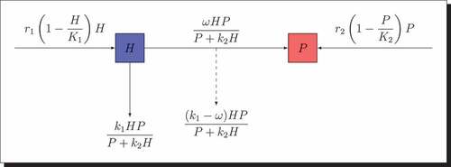
Thus, biological schematic of the model (2) is given by interaction diagram Figure 1.

Figure 1. Interaction diagram for the prey-predator model.

According to Figure 1 at any time $t>0$, we obtain the following nonlinear differential system defined by..

(2) $\left\{\begin{array}{cc}\frac{dH}{dt}=& r_1\left(1-\frac{H}{K_1}\right)H-\frac{k_{1}HP}{P+k_{2}H},H(0)=H_0>0,\\ \frac{dP}{dt}=& r_2\left(1-\frac{P}{K_2}\right)P+\frac{\omega HP}{P+k_{2}H},P(0)=P_0>0,\end{array}\right.$(2)

where

• $r_1,r_2>0$ are respectively prey and the predator growth-rates,

• $K_1,K_2>0$ represent respectively the carrying capacity of the prey and the predator,

• $k_1$ and $k_2$ represent respectively predator search and satiety rates,

• $e=\frac{\omega }{k_1}$ represents the conversion rate of prey biomass into predatory biomass, with $0<e<1$,

• $\omega$ represents predator growth-rate due to prey consummation,

• $\frac{(k_1-\omega )HP}{P+k_{2}H}$ is a residual term and represents the quantity of prey taken by predators and which did not contribute to the growth of predators.

2.2. The epidemiological model

In this section, we aim to establish a prey-predator model when the disease spread in the two populations. We assume that the disease can be transmitted vertically and horizontally. Indeed, for this study, a predator can become infected either by eating an infected prey or by contact with an infected predator. It should be noted that the density dependence affects not only births but also the deaths in the populations. Thus, we need to separate the effects of the density dependence. The parameter ${\theta }_i,i=1,2$ is such that $\left(b_i-\frac{r_i{\theta }_{i}H}{K_i}\right)$ and ${\mu }_i+\frac{(1-{\theta }_i)r_{i}H}{K_i}$ are respectively the birth and mortality rate, $b_i,{\mu }_i,i=1,2$ are respectively the natural birth and death rates coefficients, $r_i=b_i-{\mu }_i,i=1,2$ is the intrinsic growth rate, ${\theta }_i,i=1,2$ represents proportion affecting births and $1-{\theta }_i,i=1,2$ represents proportion affecting deaths. For $0<{\theta }_i<1,i=1,2$ the birth rate decreases and the death rate increases as $H$ and $P$ increases to their carrying capacity $K_i,i=1,2$. The birth rate is density independent when ${\theta }_i=0,i=1,2$ and the death rate is density independent when ${\theta }_i=1,i=1,2$.

For this study, we assume moreover that reproduction takes place only among susceptible predators.

The SIS compartmental model in epidemiology with standard incidence is given by Tewa et al. (2013)

(3) $\left\{\begin{array}{ccc}\dot{S}& =& b-\mu S-\lambda \frac{IS}{N}+\sigma I,\\ \dot{I}& =& \lambda \frac{IS}{N}-\sigma I-\mu I,\end{array}\right.$(3)

where

• $S$ and $I$ denote respectively the susceptible and infectious population,

• $N=S+I$ represents the total population,

• $\sigma$ and $\mu$ represent respectively the recovery rate of infectious individuals and the mortality death rate,

• $b$ and $\lambda$ represent respectively recruitments in susceptible compartment and the adequate contact rate between susceptible and infectious.

The following basic assumptions hold for our models:

• $(H_4)$: In the absence of infection and predation, the prey population grows logistically.

• $(H_5):$ The disease spreads horizontally and vertically with standard incidence $\lambda \frac{IS}{N}$.

• $(H_6):$ The disease is not genetically inherited. The infected population does not recover or become immune.

• $(H_7):$ We assume that only susceptible prey and predator is capable of reproducing and contributing to their carrying capacity.

• $(H_8):$ We assume that predator cannot distinguish infected and healthy prey.

• $(H_9):$ We assume that the presence of infected preys is compensated by the presence of infected predators.

Then, the biological schematic of model (4) is presented in Figure 2, where,

Figure 2. Interaction diagram for the prey-predator model when the disease spreads in the two populations.

• $f_1=r_{1}H\left(1-\frac{H}{K_1}\right),f_2=\frac{(k_1-k_2)P}{P+k_{2}H},f_3=b_1-\frac{r_1{\theta }_{1}H}{K_1},f_4=\frac{k_{1}P}{P+k_{2}H}$

• $\begin{array}{rl}& f_5=f_6=\frac{k_{1}H}{P+k_{2}H},f_7=f_8={\mu }_1+\frac{(1-{\theta }_1)r_{1}H}{K_1},\\ & f_9=f_{10}={\mu }_2+\frac{(1-{\theta }_2)r_{2}P}{K_2}\end{array}$

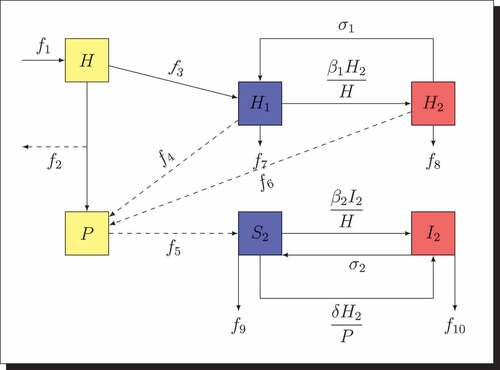
According to the above assumptions and to Figure 2, we get the following epidemic model:

(4) $\left\{\begin{array}{c}{\dot{H}}_1=\left(b_1-\frac{r_1{\theta }_{1}H}{K_1}\right)H-\left[{\mu }_1+\frac{(1-{\theta }_1)r_{1}H}{K_1}\right]H_1-{\beta }_1\frac{H_1{H}_2}{H}\\ +{\sigma }_1{H}_2-\frac{k_1{H}_{1}P}{P+k_{2}H},{\dot{H}}_2={\beta }_1\frac{H_1{H}_2}{H}-{\sigma }_1{H}_2-\left[{\mu }_1+\frac{(1-{\theta }_1)r_{1}H}{K_1}\right]\\ H_2-\frac{k_1{H}_{2}P}{P+k_{2}H},{\dot{S}}_2=\left(b_2-\frac{r_2{\theta }_{2}P}{K_2}\right)P+\frac{\omega HP}{P+k_{2}H}-\delta \frac{S_2{H}_2}{P}\\ -\left[{\mu }_2+\frac{(1-{\theta }_2)r_{2}P}{K_2}\right]S_2-{\beta }_2\frac{S_2{I}_2}{P}+{\sigma }_2{I}_2,{\dot{I}}_2={\beta }_2\frac{S_2{I}_2}{P}+\delta \frac{S_2{H}_2}{P}\\ -\left[{\mu }_2+\frac{(1-{\theta }_2)r_{2}P}{K_2}\right]I_2-{\sigma }_2{I}_2,\end{array}\right.$(4)

where,

• $H_1$ and $H_2$ represent respectively the density of susceptible and infected prey,

• $I_1$ and $I_2$ represent respectively the density of susceptible and infected predator,

• $H=H_1+H_2$ and $P=S_2+I_2$ represent respectively the total prey and predators population,

• ${\beta }_i,i=1,2$ represent the adequate contact rate between susceptible and infectious,

• ${\sigma }_i,i=1,2$ is the recover rate of infectious individuals to become susceptible,

• $\delta$ is the contact rate between susceptible predators and infectious preys.

Remark 2.1. It is important to note that the sum of the equations of the epidemic model (4) gives the ecological model (2). Moreover, since $H_1=H-H_2$ and $S_2=P-I_2$, the study of system (4) is equivalent to the coupling of differential equations in $H_2$, $I_2$ and system (2).

Thus, the complete eco-epidemiological model is given by the following differential system:

(5) $\left\{\begin{array}{c}\dot{H}=\left[r_1\left(1-\frac{H}{K_1}\right)-\frac{k_{1}P}{P+k_{2}H}\right]H,\\ \stackrel{.}{H_2}=\left[{\beta }_1\frac{(H-H_2)}{H}-{\sigma }_1-\left[{\mu }_1+\frac{(1-{\theta }_1)r_{1}H}{K_1}\right]-\frac{k_{1}P}{P+k_{2}H}\right]H_2,\\ \dot{P}=\left[r_2\left(1-\frac{P}{K_2}\right)+\frac{\omega H}{P+k_{2}H}\right]P,\\ \stackrel{.}{I_2}={\beta }_2\frac{(P-I_2)I_2}{P}+\delta \frac{(P-I_2)H_2}{P}-\left[{\mu }_2+\frac{(1-{\theta }_2)r_{2}P}{K_2}\right]I_2-{\sigma }_2{I}_2.\end{array}\right.$(5)

3. Mathematical analysis

3.1. The mathematical analysis of the baseline model

This section deals with mathematical analyses including the stability and the bifurcation analyses of system (2) (Traoré et al., 2019, 2018). Then, we rewrite model (2) in the following form:

$\dot{X}(t)=F(X(t)),$

where $X(t)=(H(t),P(t){)}^T$ and $F$ are defined on ${\mathbb{R}}^2$ by:

$F(X)=\left(\begin{array}{c}{F}_1(N,P)\\ F_2(N,P)\end{array}\right)=\left(\begin{array}{c}{r}_1\left(1-\frac{H}{K_1}\right)H-\frac{k_{1}HP}{P+k_{2}H}\\ r_2\left(1-\frac{P}{K_2}\right)P+\frac{\omega HP}{P+k_{2}H}\end{array}\right)$

The preliminary results, concern the existence, positiveness, boundedness and uniform persistence of solutions of system (2).

3.1.1. Existence, positiveness, boundedness and uniform persistence of solutions

From a biological point of view, it is important to show the existence, positivity and boundedness of the solution of system (2).

Theorem 3.1. (Existence of solutions) System (2) admits a unique global solution $(H(t),P(t))$ defined in interval $[0,T_{max}[$.

Proof. Indeed, the theorem of Cauchy-Lipschitz, (Koutou, Traoré, Sangaré et al., 2018a; Savadogo et al., 2021; Traoré et al., 2019, 2018; Xia et al., 1996) assures the existence and uniqueness of local solution of system (2) on $[0,T_{max}[$ given the regularity of the functions involved in the model.

Theorem 3.2. (Positivity) The nonnegative orthant ${\mathbb{R}}_{+}^2$ is positively invariant by system (2).

Proof. Indeed, to show the positive invariance of the positive orthant under the flow of system (2); it suffices to show that the axes $H=0$ and $P=0$ of the positive orthant cannot be crossed. Assume that initially, all variables are nonnegative.

1. Let a point $X_0=(0,p_0)$ belongs to the axis $H=0.$ Its orbits take the following form

${\mathcal{D}}_{X_0}=\{(0,p(t)),t\in {\mathbb{R}}_{+}\}.$

So axis $H=0$ cannot be crossed from positive to negative $H$.

1. Let a point $Y_0=(h_0,0)$ belongs to the axis $P=0.$ Its orbits take the following form

${\mathcal{D}}_{Y_0}=\{(h(t),0),t\in {\mathbb{R}}_{+}\}$

So axis $P=0$ cannot be crossed.

So, an orbit that begins in this orthant remains inside. Thus, the nonnegative orthant ${\mathbb{R}}_{+}^2$ is positively invariant for system (2).

Proposition 3.1. The set

$D:=\{(H,P)\in {\mathbb{R}}_{+}^2/H\le K_1,P\le K_c\}where{K}_c=K_2\left(1+\frac{\omega }{r_2{k}_2}\right)$

is positively invariant and absorbing for system (2).

Proof. Indeed,

1. Let define $D_0=\{(H,P)\in {\mathbb{R}}_{+}^2/H\le K_1\}$ and $D_1=\{(H,P)\in {\mathbb{R}}_{+}^2/P\le K_c\}$ and show that $D_0$ and $D_1$ are positively invariant and absorbing for system (2).

$D_0$ is positively invariant. Indeed, let $f_1$ the function defined on ${\mathbb{R}}^2$ by $f_1(H,P)=H-K_1,$ we have

$\mathrm{\nabla }{f}_1(H,P)=\left(\begin{array}{c}1\\ 0\end{array}\right)\ne 0_{{\mathbb{R}}^2}\mathrm{a}\mathrm{n}\mathrm{d}⟨\mathrm{\nabla }{f}_1|F⟩=-\frac{k_1{K}_{1}P}{P+k_2{K}_1}.$

Thus $⟨\mathrm{\nabla }{f}_1|F⟩\le 0$ on $\{(H,P)\in {\mathbb{R}}_{+}^2/H=K_1\}.$

Therefore, $D_0$ is positively invariant. Let show that $D_0$ is absorbing. Consider the differential inequality defined by

$\frac{dH}{dt}\le r_1\left(1-\frac{H}{K_1}\right)H,$

and by using the principle of comparison, we deduce that $\underset{t\to +\mathrm{\infty }}{lim}supH(t)\le K_1$. Hence for $\in >0$, there exists $T>0$ such that $H(t)\le \underset{t\ge T}{sup}H(t)\le K_1+\in$; as $\in$ is arbitrary we deduce that $D_0$ is absorbing. Consequently, $D_0$ is positively invariant and absorbing.

Now, let us show that

$P\le K_c.$

Indeed, consider the second equation of system (2),

$\frac{dP}{dt}=r_2\left(1-\frac{P}{K_2}\right)P+\frac{\omega HP}{P+k_{2}H},\mathrm{f}\mathrm{o}\mathrm{r}t\ge T,\frac{\omega H}{P+k_{2}H}<\frac{\omega }{k_2}$

Thus, we obtain the following differential inequality,

(6) $\frac{dP}{dt}\le \left(r_2\left(1-\frac{P}{K_2}\right)+\frac{\omega }{k_2}\right)P,\mathrm{\forall }t\ge t_0$(6)

According to the comparison principle, we deduce that

(7) $\underset{t\to +\mathrm{\infty }}{lim}sup(P(t))\le K_2\left(1+\frac{\omega }{r_2{k}_2}\right)=K_c$(7)

Thus, $D_1$ is positively invariant and absorbing.

Finally, we conclude that $D$ is positively invariant and absorbing for system (2).

To show the global existence of solutions, we must show that the solutions of the system are bounded. In the previous demonstration we have established that $H$ and $P$ are bounded. Thus, we can conclude that the solutions of system (2) exist globally.

For the study of system (2), we restrain a set defined by:

$\mathcal{D}=\{(H,P)\in {\mathbb{R}}_{+}^2/0\le H\le K_1,0\le P\le K_c\}$

Now, we are in a position to show the uniform persistence of the system. Indeed, uniform persistence, ensures the long term survival of all populations (prey and predator) no matter what the initial populations are. Now, we give a result guaranteeing the uniform persistence of system (2; Haijiao & Shangjiang, 2017; Subhas, 2017; Traoré et al., 2019, 2018).

Theorem 3.3. System (2) is uniformly persistence if $r_1>k_1.$

Proof. Indeed, from the first equation of system (2) we have,

$\frac{dH}{dt}\ge \frac{r_1}{K_1}H\left[(r_1-k_1)\frac{K_1}{r_1}-H\right]\Rightarrow \underset{t\to +\mathrm{\infty }}{liminf}H(t)=(r_1-k_1)\frac{K_1}{r_1}=\underset{\_}{H(t)}\mathrm{a}\mathrm{c}\mathrm{c}\mathrm{o}\mathrm{r}\mathrm{d}\mathrm{i}\mathrm{n}\mathrm{g}\mathrm{t}\mathrm{o}{r}_1>k_1.$

Now, from the second equation of system (2) we have

$\frac{dP}{dt}=r_{2}P-\frac{r_2}{K_2}{P}^2=\frac{1}{K_2}P\left(K_2-P\right)\Rightarrow \underset{t\to +\mathrm{\infty }}{liminf}P(t)=K_2=\underset{\_}{P(t)}.$

Hence, system (2) is uniformly persistent.

3.1.2. Stability analysis of trivial equilibria

System (2) has three biologically meaningful equilibrium points. When the populations are at equilibrium state, they do not move further. The equilibrium states are obtained from the nullclines of model (2). The trivial equilibrium of system (2) is given by the following proposition:

Proposition 3.2. The equilibrium points are:

1. $E_1=(K_1,0)$ is trivial equilibrium state of system (2),

1. $E_2=\left(0,K_2\right)$ is trivial equilibrium state of system (2).

Proof. Indeed, to get the equilibrium point, we solve the following system:

(8) $\left\{\begin{array}{c}{r}_1\left(1-\frac{H}{K_1}\right)H-\frac{k_{1}HP}{P+k_{2}H}=F_1(H,P)=0,\\ \hspace{0.17em}\\ r_2\left(1-\frac{P}{K_2}\right)P+\frac{\omega HP}{P+k_{2}H}=F_2(H,P)=0.\end{array}\right.$(8)

1. $F_1(K_1,0)=F_2(K_1,0)=0.$ Thus, $E_1=(K_1,0)$ is the trivial equilibrium point.

2. In the same way, $F_1\left(0,K_2\right)=F_2\left(0,K_2\right)=0.$ Then, $E_2=\left(0,K_2\right)$ is an equilibrium point of system (2).

Now, we are in position to investigate the local stability analysis of the trivial equilibrium points. The local stability of trivial equilibrium points is given by the following proposition.

Proposition 3.3.

1. $E_1$ is always unstable,

1. $E_2$ is locally asymptotically stable if and only if $r_1<k_1$.

Proof. Indeed, the local stability analysis of system (2) around each of the two equilibria is obtained by calculating the variational matrix corresponding to each equilibrium point. The variational matrix of system (2) is

$J(X)=\left(\begin{array}{cc}{r}_1\left(1-\frac{2H}{K_1}\right)-\frac{k_1{P}^2}{{(P+k_{2}H)}^2}& -\frac{k_1{H}^2}{P+k_{2}H}\\ \frac{\omega P^2}{{(P+k_{2}H)}^2}& r_2\left(1-\frac{2P}{K_2}\right)+\frac{\omega H^2}{{(P+k_{2}H)}^2}\end{array}\right).$

1. At the equilibrium point $E_1$ the variational matrix $J(E_1)$ is given by

$J(E_1)=\left(\begin{array}{cc}-r_1& -\frac{k_1}{k_2^2}\\ 0& r_2+\frac{\omega }{k_2^2}\end{array}\right).$

The eigenvalues are ${\lambda }_1=-r_1<0$ and ${\lambda }_2=r_2+\frac{\omega }{k_2^2}>0$, which indicate that the equilibrium $E_1$ is an unstable one. In this case, we have stability of prey and instability of predator.

1. The variational matrix of system (2) evaluated at $E_2$ is given by

$J(E_2)=\left(\begin{array}{cc}{r}_1-k_1& 0\\ \omega & -r_2\end{array}\right)$

The corresponding eigenvalues are ${\lambda }_1=r_1-k_1$ and ${\lambda }_2=-r_2.$ Then, if $r_1<k_1$ then $E_2$ is locally asymptotically stable.

3.1.3. Existence and stability analysis of coexistence equilibria

We define the following quadratic function $\pi$ on ${\mathbb{R}}_{+}^{\ast }$ by

(9) $\pi (X)=A_2{X}^2+A_{1}X+A_0=0$(9)

where,

$A_0=K_1{K}_2(\omega +r_2{k}_1{K}_1{k}_2)(k_1-r_1),$

$A_1=(\omega +r_1{k}_1{K}_1{r}_2{k}_2)K_2-r_1{r}_2{k}_1{K}_1^2{k}_2^2,$

$A_2=r_1{r}_2{k}_1{K}_1{k}_2^2.$

The following result gives the existence of coexistence equilibrium.

Theorem 3.4. System (2) admits a unique coexistence equilibrium $E_3=(H^{\ast },P^{\ast })$ if the following conditions are satisfied..

1. $\frac{r_1(K_1-H^{\ast })}{k_1{K}_1}<1,$

1. $r_1>k_1,$ $\frac{(\omega +r_1{k}_1{K}_1{r}_2{k}_2)K_2}{r_1{r}_2{k}_1{K}_1^2{k}_2^2}>1,$

1. $(\omega +r_1{k}_1{K}_1{r}_2{k}_2)K_2=r_1{r}_2{k}_1{K}_1^2{k}_2^2$ and $r_1>k_1.$

Proof. Indeed, the equilibrium points are solutions of system (2)

(10) $\left\{\begin{array}{c}{r}_1\left(1-\frac{H}{K_1}\right)H-\frac{k_{1}HP}{P+k_{2}H}=F_1(H,P)=0,\\ r_2\left(1-\frac{P}{K_2}\right)P+\frac{\omega HP}{P+k_{2}H}=F_2(H,P)=0.\end{array}\right.$(10)

From $F_1(H^{\ast },P^{\ast })=0$ and dividing by $H^{\ast }$, we get $P^{\ast }=\frac{r_1{k}_2(K_1-H^{\ast })H^{\ast }}{k_1{K}_1-r_1(K_1-H^{\ast })}.$

According to $i)$ of Theorem 3.4, we have $P^{\ast }>0.$

By plugging $P^{\ast }$ in $F_1(H^{\ast },P^{\ast })=0$, we obtain equation (9)(9) $\pi (X)=A_2{X}^2+A_{1}X+A_0=0$(9)

According to $r_1>k_1$, we have $A_1^2-4A_0{A}_2>0,$ thus equation $\pi (X)=0$ has two roots

$H_1^{\ast }=\frac{-A_1+\sqrt{A_1^2-4A_0{A}_2}}{2A_2}\mathrm{a}\mathrm{n}\mathrm{d}{H}_2^{\ast }=\frac{-A_1-\sqrt{A_1^2-4A_0{A}_2}}{2A_2}.$

According to $r_1>k_1$ and $\frac{(\omega +r_1{k}_1{K}_1{r}_2{k}_2)K_2}{r_1{r}_2{k}_1{K}_1^2{k}_2^2}>1,$ we have respectively $A_0<0$ and $A_1>0.$ Thus, $H_1^{\ast }>0$ and $H_2^{\ast }<0.$ Consequently, system (2) has a unique coexistence equilibrium. According to $(\omega +r_1{k}_1{K}_1{r}_2{k}_2)K_2=r_1{r}_2{k}_1{K}_1^2{k}_2^2$ we have $H^{\ast }=\frac{\sqrt{-A_0{A}_2}}{A_2}.$ By using $r_1>k_1$, we get $H^{\ast }>0.$ Consequently, system (2) has unique coexistence equilibrium.

Concerning the local behavior of system (2) around coexistence equilibrium $E_3=(H^{\ast },P^{\ast })$, we state the following theorem giving the local stability of coexistence equilibrium.

Theorem 3.5 If $r_1>k_1$, $\frac{r_1(K_1-H^{\ast })}{k_1{K}_1}<1$ and if

(11) $\frac{{(k_1{k}_2)}^2{H}^{\ast }(k_1{k}_2{K}_1^2+H^{\ast })+e{K}_1^2{(k_1{K}_1-r_1(K_1-H^{\ast }))}^2}{{(k_1{k}_2)}^2{K}_1{H}^{\ast }(1+2k_1{k}_2{K}_1{H}^{\ast })}>1$(11)

and

(12) $\frac{{(k_2{H}^{\ast })}^2+K_1{H}^{\ast }+k_1{k}_2{K}_1^2(1+K_1)+2k_2^2{K}_1}{k_1{k}_2{K}_1(1+2K_1)H^{\ast }+K_1(1+k_2^2{K}_1)}<1$(12)

then the coexistence equilibrium $E_3=(H^{\ast },P^{\ast }),$ is locally asymptotically stable.

Proof. Indeed, the Jacobian matrix of system (2) around $E_3$ is given by..

$J(E_3)=\left(\begin{array}{cc}{a}_{11}^{\ast }& a_{12}^{\ast }\\ a_{21}^{\ast }& a_{22}^{\ast }\end{array}\right)$

$a_{11}^{\ast }=\frac{r_1(k_1{K}_1-r_1(K_1-H^{\ast }))(K_1-H^{\ast })}{k_1{K}_1^3}$, $a_{12}^{\ast }=-\frac{{(k_1{K}_1-r_1(K_1-H^{\ast }))}^2}{{(k_1{K}_1)}^2{k}_2^3},$

$a_{21}^{\ast }=\frac{e{r}_1(K_1-H^{\ast })(k_1{K}_1-r_1(K_1-H^{\ast }))}{k_1^2{K}_1{H}^{\ast }},$ $a_{22}^{\ast }=\frac{r_1(k_1{k}_2{K}_1^2+H^{\ast })-r_1{K}_1(1+2k_1{k}_2{H}^{\ast })}{k_1{k}_2{K}_1^2}.$

The characteristic polynomial is therefore:

$P(X)=X^2-B_{1}X+B_2=0,$

where

$B_1=\mathrm{t}\mathrm{r}(J(E_3))=a_{11}^{\ast }+a_{22}^{\ast },$

$B_2=\mathrm{d}\mathrm{e}\mathrm{t}(J(E_3))=a_{11}^{\ast }{a}_{22}^{\ast }-a_{12}^{\ast }{a}_{21}^{\ast }.$

According to the expression of (11) and (12), we get respectively $det(J(E_3))>0$ and $\mathrm{t}\mathrm{r}(J(E_3))<0.$ By applying the Routh-Hurwitz criterion, $E_3$ is locally asymptotically stable.

Now, we perform the global dynamics equilibrium point $E_3$ by constructing a suitable Lyapunov function (Chiu, 1999; Rosenzweig & MacArthur, 1963; Savadogo et al., 2021; Tozzi & Peters, 2019; Traoré et al., 2019, 2018).

Theorem 3.6. According to Theorem 3.3 and if $\frac{r_1(K_1-H^{\ast })}{k_1{K}_1}<1$, the coexistence equilibrium point $E_3=(H^{\ast },P^{\ast })$ is globally asymptotically stable on

$\mathrm{\Omega }=\{(H,P)\in {\mathbb{R}}_{+}^2/0<H<H^{\ast }\le K_1,0<P<P^{\ast }\le K_c\}.$

Proof. Indeed, we construct a Lyapunov candidate function defined on $\mathrm{\Omega }$ by:

$V(H,P)=V_1(H)+V_2(P),$

with $V_1(H)=a_1{\int }_{H^{\ast }}^H\frac{\zeta -H^{\ast }}{\zeta }d\zeta$, $V_2(P)=a_2{\int }_{P^{\ast }}^P\frac{\zeta -P^{\ast }}{\epsilon }d\epsilon$, and $(a_1,a_2)\in {\mathbb{R}}_{+}^{\ast 2}$ to be determined. It is easy to see that $V(H^{\ast },P^{\ast })=0$ and for all $(H,P)\in C\mathrm{\setminus }\{E_3\}$, $V(H,P)>0.$ So $V$ is well defined on $\mathrm{\Omega }$.

The time derivative of $V(H,P)$ along the solutions of system (2) is given by the expression:

$\dot{V}(N,P)=a_1\dot{H}\left(\frac{H-H^{\ast }}{H}\right)+a_2\dot{P}\left(\frac{P-P^{\ast }}{P}\right)$

$=a_1(H-H^{\ast })\left[r_1\left(1-\frac{H}{K_1}\right)-\frac{k_{1}P}{P+k_{2}H}\right]+a_2(P-P^{\ast })\left[r_2\left(1-\frac{P}{K_2}\right)+\frac{\omega H}{P+k_{2}H}\right].$

After simplification, we can write

$\dot{V}(H,P)=a_1(H-H^{\ast }{)}^2\left[-\frac{r_1}{K_1}+\frac{k_1{k}_2{P}^{\ast }}{(P^{\ast }+k_2{H}^{\ast })(P+k_{2}H)}\right]-\frac{a_1{k}_1{k}_2{H}^{\ast }(H-H^{\ast })(P-P^{\ast })}{(P^{\ast }+k_2{H}^{\ast })(P+k_{2}H)}$

$+a_2(P-P^{\ast }{)}^2\left[-\frac{r_2}{K_2}-\frac{\omega H^{\ast }}{(P+k_{2}H)(P^{\ast }+k_2{H}^{\ast })}\right]+\frac{a_2\omega P^{\ast }(H-H^{\ast })(P-P^{\ast })}{(P+k_{2}H)(P^{\ast }+k_2{H}^{\ast })}.$

Set up $a_1=1$ and $a_2=\frac{k_1{k}_2{H}^{\ast }}{P^{\ast }},$ and using the fact that $\frac{1}{P+k_{2}H}<1$, we have finally

$\dot{V}(N,P)=(H-H^{\ast }{)}^2\left[-\frac{r_1}{K_1}+\frac{r_1{k}_2(K_1-H^{\ast })}{K_1(P+k_{2}H)}\right]$

$+a_2(P-P^{\ast }{)}^2\left[-\frac{r_2}{K_2}-\frac{\omega H^{\ast }}{(P+k_{2}H)(P^{\ast }+k_2{H}^{\ast })}\right].$

$<(H-H^{\ast }{)}^2\left[\frac{r_1(k_2(K_1-H^{\ast })-1)}{K_1}\right]$

$+a_2(P-P^{\ast }{)}^2\left[-\frac{r_2}{K_2}-\frac{e(k_1{K}_1-r_1(K_1-H^{\ast }))}{k_2{K}_1(P+k_{2}H)}\right].$

The coefficients $(H-H^{\ast }{)}^2$ and $(P-P^{\ast }{)}^2$ are positive for all $(H,P)\in C\mathrm{\setminus }\{E_3\}$.

So, according to $\frac{r_1(K_1-H^{\ast })}{k_1{K}_1}<1$, $\dot{V}(H,P)<0$.

In addition $\dot{V}(H,P)=0$ if and only if $(H,P)=(H^{\ast },P^{\ast }).$ By using LaSalle invariance principle, $E_3=(H^{\ast },P^{\ast })$ is globally asymptotically stable on $\mathrm{\Omega }$.

3.1.4. Analysis of Hopf Bifurcation diagram at $E_3$

Here, our results are based on (Bairagi et al., 2007; Koutou et al., 2021; Ouedraogo et al., 2019; Xiao & Chen, 2001) approach. It is remarked that system (2) is sensitive to perturbation of predation rate. As small change of this parameter transforms stable coexisting populations into a disturbed system. This phenomenon of disturbance is a kind of instability in the system. So, we analyze the system for this factor which could lead to destabilization. Hopf bifurcation is one of a kind of instability. Bifurcation analysis gives information about the long-term dynamic behavior of nonlinear dynamic systems. Then, $k_1$, the rate of predation is the bifurcation parameter. The necessary and sufficient conditions for Hopf Bifurcation to occur at $k_1=k_{1c}$ are given by:

(13) $(L_1):B_2(k_{1c})>0,$(13)

(14) $(L_2):F(k_{1c})=a_{11}^{\ast }(k_{1c})+a_{22}^{\ast }(k_{1c})=0,$(14)

(15) $(L_3):Re{\left[\frac{dF(k_1)}{d{k}_1}\right]}_{k_1=k_{1c}}\ne 0.$(15)

Using the fact that $a_{11}^{\ast }+a_{22}^{\ast }=0$ we have,

$\frac{r_1(k_1{K}_1-r_1(K_1-H^{\ast }))(K_1-H^{\ast })}{k_1{K}_1^3}+\frac{r_1(k_1{k}_2{K}_1^2+H^{\ast })-r_1{K}_1(1+2k_1{k}_2{H}^{\ast })}{k_1{k}_2{K}_1^2}=0$

The following theorem gives the condition of Hopf bifurcation occur at $k_1=k_{1c}$.

Theorem 3.7. If $r_1>k_1$, $\frac{r_1(K_1-H^{\ast })}{k_1{K}_1}<1$, and

(16) $\frac{{(k_1{k}_2)}^2{H}^{\ast }(k_1{k}_2{K}_1^2+H^{\ast })+e{K}_1^2{(k_1{K}_1-r_1(K_1-H^{\ast }))}^2}{{(k_1{k}_2)}^2{K}_1{H}^{\ast }(1+2k_1{k}_2{K}_1{H}^{\ast })}>1,$(16)

then an Hopf bifurcation occurs at value $k_1=k_{1c}$ where

$k_{1c}=\frac{K_1(1+k_2^2{K}_1+H^{\ast })-k_2(2k_2{K}_2+H^{{\ast }^2})}{K_1(k_2{K}_1(1+K_1)-k_2{H}^{\ast }(1+2K_1))}$

Proof. The characteristic polynomial associated with $E_3=(H^{\ast },P^{\ast })$ is given by:

$P(X)=X^2-B_1(k_1)X+B_2(k_1)=0$

with

$B_1(k_1)=a_{11}^{\ast }+a_{22}^{\ast }.$

$B_2(k_1)=a_{11}^{\ast }{a}_{22}^{\ast }-a_{12}^{\ast }{a}_{21}^{\ast }.$

According to condition (16), $B_2(k_1)>0$, for all positive values of $k_1.$

Set up

$F(k_1)=a_{11}^{\ast }+a_{22}^{\ast }.$

It is straightforward to see that $F(k_{1c})=0$ (condition of non-degeneration).

Now, let verify the transversality condition. We have,

${\left(\frac{dF(k_1)}{d{k}_1}\right)}_{k_1=k_{1c}}=\frac{(K_1-H^{\ast })(r_1{k}_2(K_1-H^{\ast })+r_1{K}_1)}{k_1^2{k}_2{K}_1^3}\ne 0.$

Therefore, the transversality conditions hold and hence the Hopf bifurcation occurs at $k_1=k_{1c}.$

Under conditions (14), (15), and (16) a simple Hopf bifurcation occurs at equilibrium point $E_3$ at some critical value $k_{1c}$.

3.2. Mathematical analysis of the eco-epidemiological model

In this subsection, we aim to establish the mathematical results of system (5).

The following results ensure the positivity of system (5; Koutou et al., 2021; Subhas, 2017; Tewa et al., 2013).

Lemma 3.1. The nonnegative orthant ${\mathbb{R}}_{+}^4$ is positively invariant by system (5) Moreover the set

$F=\{(H,H_2,P,I_2)\in {\mathbb{R}}_{+}^4/0\le H_2\le H,0\le I_2\le P\},$

is positively invariant and absorbing.

Now, let us consider the following thresholds

• $R_{01}=\frac{{\beta }_1}{b_1+{\sigma }_1-r_1{\theta }_1},R_{02}=\frac{{\beta }_2}{{\mu }_2+{\sigma }_2+\frac{(1-{\theta }_2)r_2{P}^{\ast }}{K_2}}$,$R_{03}=\frac{{\beta }_1}{{\mu }_1+{\sigma }_1+\frac{(1-{\theta }_1)r_1{H}^{\ast }}{K_1}+\frac{k_1{P}^{\ast }}{P^{\ast }+k_2{H}^{\ast }}}.$

We give ecological interpretation of these threshold parameters. Thus,

1. $R_{01}$ represents the basic reproduction number of preys when there is no predator.

1. $R_{02}$ represents the basic reproduction number of predators when there is no prey.

1. $R_{03}$ represents the basic reproduction number of preys and predators when the two populations coexist.

3.2.1. Stability analysis of trivial equilibria

The equilibrium points of system (5) are given in the following proposition:

Proposition 3.4. The trivial equilibria point of system (5) are:

1. $E_1=(K_1,0,0,0)$ which always exists.

1. $E_2=\left(K_1,K_1\left(1-\frac{1}{R_{01}}\right),0,0\right)$ which is admissible if $R_{01}>1.$

1. $E_3=\left(H^{\ast },0,P^{\ast },0\right)$ exist if $\frac{r_1(K_1-H^{\ast })}{k_1{K}_1}<1$.

1. $E_4=\left(H^{\ast },0,P^{\ast },P^{\ast }\left(1-\frac{1}{R_{02}}\right)\right)$ which is admissible if $R_{02}>1$, and

$\frac{r_1(K_1-H^{\ast })}{k_1{K}_1}<1$

.

Proposition 3.5.

1. $E_3$ is locally asymptotically stable if $R_{02}<1$, $R_{03}<1$, $r_1>k_1$, $\frac{r_1(K_1-H^{\ast })}{k_1{K}_1}<1$ and if conditions (11) and (12) are satisfied.

1. $E_4$ is locally asymptotically stable if $R_{02}>1$, $R_{03}<1$, $r_1>k_1$ and conditions (11) and (12) are satisfied.

Proof. Let us consider the variational matrix of system (5):

$J(H,H_2,P,I_2)=\left(\begin{array}{cccc}{C}_{11}& 0& C_{13}& 0\\ C_{21}& C_{22}& C_{23}& 0\\ C_{31}& 0& C_{33}& C_{44}\\ 0& C_{42}& C_{43}& C_{44}\end{array}\right)$

where:

$C_{11}=r_1\left(1-\frac{2H}{K_1}\right)-\frac{k_1{P}^2}{{(P+k_{2}H)}^2}$, $C_{12}=0$, $C_{13}=-\frac{k_1{k}_2{H}^2}{{(P+k_{2}H)}^2}$, $C_{14}=0,$

$C_{21}={\beta }_2\frac{H_2^2}{H^2}-\frac{(1-{\theta }_1)r_1{H}_2}{K_1}+\frac{k_1{k}_2{H}_{2}P}{{(P+k_{2}H)}^2}$

,

$C_{22}={\beta }_1\left(1-\frac{2H_2}{H}\right)-\left({\mu }_1+{\sigma }_1+\frac{(1-{\theta }_1)r_{1}H}{K_1}\right)-\frac{k_{1}P}{P+k_{2}H}$, $C_{23}=-\frac{k_1{k}_{2}H{H}_2}{{(P+k_{2}H)}^2}$,

$C_{24}=0,$ $C_{31}=\frac{\omega P^2}{{(P+k_{2}H)}^2},$ $C_{32}=0,$ $C_{33}=r_2\left(1-\frac{2P}{K_2}\right)+\frac{\omega H^2}{{(P+k_{2}H)}^2},$

$C_{34}=0$, $C_{41}=0$, $C_{42}=\frac{\delta (P-I_2)}{P},$ $C_{43}=\frac{{\beta }_2{I}_2^2+\delta I_2{H}_2}{P^2}-\frac{(1-{\theta }_2)r_2{I}_2}{K_2},$

$C_{44}=\frac{-2{\beta }_2{I}_2-\delta H_2}{P}+{\beta }_2-\left({\mu }_2+{\sigma }_2+\frac{(1-{\theta }_2)r_{2}P}{K_2}\right).$

1. The local stability of the equilibrium $E_3=(H^{\ast },0,P^{\ast },0)$ is given by the Jacobian matrix $J(E_3)$ of system (5) evaluated at this point. We have:

$J(E_3)=\left(\begin{array}{cccc}{D}_{11}^{\ast }& 0& D_{13}^{\ast }& 0\\ 0& {\beta }_1\left(1-\frac{1}{R_{03}}\right)& 0& 0\\ D_{31}^{\ast }& 0& D_{33}^{\ast }& 0\\ 0& \delta & 0& D_{44}^{\ast }\end{array}\right).$

where

$D_{11}^{\ast }=\frac{r_1(k_1{K}_1-r_1(K_1-H^{\ast }))(K_1-H^{\ast })}{k_1{K}_1^3}$, $D_{12}^{\ast }=0$, $D_{13}^{\ast }=-\frac{{(k_1{r}_1-r_1(K_1-H^{\ast }))}^2}{K_1^2}$,

$D_{14}^{\ast }=0,$ $D_{21}^{\ast }=0$, $D_{22}^{\ast }={\beta }_1\left(1-\frac{1}{R_{03}}\right)$, $D_{23}^{\ast }=0$, $D_{24}^{\ast }=0,$

$D_{31}^{\ast }=\frac{e{r}_1(K_1-H^{\ast })(k_1{K}_1-r_1(K_1-H^{\ast }))}{k_1{H}^{\ast }{K}_1^2},$ $D_{32}^{\ast }=0,$

$D_{33}^{\ast }=\frac{r_1(k_1{k}_2{K}_1^2+H^{\ast })-r_1{K}_1(1+2k_1{k}_2{H}^{\ast })}{k_1{k}_2{K}_1^2},$ $D_{34}^{\ast }=0$, $D_{41}^{\ast }=0$, $D_{42}^{\ast }=\delta ,$ $D_{43}^{\ast }=0,$ $D_{44}^{\ast }={\beta }_2\left(1-\frac{1}{R_{02}}\right).$

The characteristic polynomial is therefore given by:

$P(\lambda )=(D_{44}^{\ast }-\lambda )\left({\beta }_1\left(1-\frac{1}{R_{03}}\right)-\lambda \right)({\lambda }^2-(D_{11}^{\ast }+D_{33}^{\ast })\lambda +D_{11}^{\ast }{D}_{33}^{\ast }-D_{31}^{\ast }{D}_{13}^{\ast }=0.$

Then, the eigenvalues of $J(E_3)$ is ${\lambda }_1=D_{44}^{\ast }$, ${\lambda }_2={\beta }_1\left(1-\frac{1}{R_{03}}\right)$. If $R_{02}<1$ and $R_{03}<1$ we have respectively ${\lambda }_1<0$ and ${\lambda }_2<0$. According to expressions (11) and (12), we find $D_{11}^{\ast }+D_{33}^{\ast }<0$ and $D_{11}^{\ast }{D}_{33}^{\ast }-D_{31}^{\ast }{D}_{13}^{\ast }>0$, by applying the Routh-Hurwitz criterion, the roots of ${\lambda }^2-(D_{11}^{\ast }+D_{33}^{\ast })\lambda +D_{11}^{\ast }{A}_{33}^{\ast }-D_{31}^{\ast }{D}_{13}^{\ast })=0$ are real part negative. Subsequently $E_3$ is locally asymptotically stable.

1. For $E_4=\left(H^{\ast },0,P^{\ast },P^{\ast }\left(1-\frac{1}{R_{02}}\right)\right)$ the associated Jacobian matrix is:

$J(E_4)=\left(\begin{array}{cccc}{E}_{11}^{\ast }& 0& E_{13}^{\ast }& 0\\ 0& {\beta }_1\left(1-\frac{1}{R_{03}}\right)& 0& 0\\ E_{31}^{\ast }& 0& E_{33}^{\ast }& 0\\ 0& E_{42}^{\ast }& E_{43}^{\ast }& E_{44}^{\ast }\end{array}\right).$

where

$E_{11}^{\ast }=\frac{r_1(k_1{K}_1-r_1(K_1-H^{\ast }))(K_1-H^{\ast })}{k_1{K}_1^3}$, $E_{12}^{\ast }=0$, $E_{13}^{\ast }=-\frac{{(k_1{r}_1-r_1(K_1-H^{\ast }))}^2}{K_1^2}$,

$E_{14}^{\ast }=0,$ $E_{21}^{\ast }=0$, $E_{22}^{\ast }={\beta }_1\left(1-\frac{1}{R_{03}}\right)$, $E_{23}^{\ast }=0$, $E_{24}^{\ast }=0,$ $E_{31}^{\ast }=\frac{e{r}_1(K_1-H^{\ast })(k_1{K}_1-r_1(K_1-H^{\ast }))}{k_1{H}^{\ast }{K}_1^2},$

$E_{32}^{\ast }=0,$ $E_{33}^{\ast }=\frac{r_1(k_1{k}_2{K}_1^2+H^{\ast })-r_1{K}_1(1+2k_1{k}_2{H}^{\ast })}{k_1{k}_2{K}_1^2}$, $E_{34}^{\ast }=0$, $E_{41}^{\ast }=0$, $E_{42}^{\ast }=\frac{\delta }{R_{02}},$

$E_{43}^{\ast }={\beta }_2{\left(\frac{I_2^{\ast }}{P^{\ast }}\right)}^2-\frac{(1-{\theta }_2)r_2{P}^{\ast }}{K_2},$ $E_{44}^{\ast }=-{\beta }_2\left(1-\frac{1}{R_{02}}\right).$

The characteristic polynomial is given therefore by:

$P(\lambda )=(E_{44}^{\ast }-\lambda )\left({\beta }_1\left(1-\frac{1}{R_{03}}\right)-\lambda \right)({\lambda }^2-(E_{11}^{\ast }+E_{33}^{\ast })\lambda +E_{11}^{\ast }{E}_{33}^{\ast }-E_{31}^{\ast }{E}_{13}^{\ast })=0.$

Then, the eigenvalues of $J(E_4)$ is ${\lambda }_1=E_{44}^{\ast }$, ${\lambda }_2={\beta }_1\left(1-\frac{1}{R_{03}}\right)$. If $R_{02}>1$ and $R_{03}<1$ we have respectively ${\lambda }_1<0$ and ${\lambda }_2<0$. According to expressions (11) and (12), we find $D_{11}^{\ast }+D_{33}^{\ast }<0$ and $D_{11}^{\ast }{D}_{33}^{\ast }-D_{31}^{\ast }{D}_{13}^{\ast }>0$, by applying the Routh-Hurwitz criterion, the roots of ${\lambda }^2-(E_{11}^{\ast }+E_{33}^{\ast })\lambda +E_{11}^{\ast }{E}_{33}^{\ast }-E_{31}^{\ast }{E}_{13}^{\ast }=0$ are real part negative. Subsequently $E_4$ is locally asymptotically stable.

Theorem 3.8. The following results hold for system (5) in the set $F.$

1. If $\underset{t\to 0}{lim}H(t)=0$ and $\underset{t\to 0}{lim}P(t)=0$ then $\underset{t\to +\mathrm{\infty }}{lim}(H,H_2,P,I_2)=E_0.$

2. If $R_{01}>1$, $\underset{t\to 0}{lim}H(t)>0$ and $\underset{t\to 0}{lim}P(t)=0$ then $\underset{t\to +\mathrm{\infty }}{lim}(H,H_2,P,I_2)=E_2.$

3. If $R_{01}\le 1$, $\underset{t\to 0}{lim}H(t)>0$ and $\underset{t\to 0}{lim}P(t)=0$ then $\underset{t\to +\mathrm{\infty }}{lim}(H,H_2,P,I_2)=E_1.$

Proof.

1. As $H(0)=0$ and $P(0)=0$ we have respectively $\underset{t\to +\mathrm{\infty }}{lim}H(t)=0$ and $\underset{t\to +\mathrm{\infty }}{lim}P(t)=0$, since the set ${\mathrm{\Omega }}_0=\{(H,H_2,P,I_2)\in {\mathbb{R}}_{+}^4/H=0,P=0\}$ is positively invariant by the flow of system (5). Since, the study of system (5) is done in $F$, thus we deduce that $\underset{t\to +\mathrm{\infty }}{lim}{H}_2(t)=\underset{t\to +\mathrm{\infty }}{lim}{I}_2(t)=0.$ Subsequently, $\underset{t\to +\mathrm{\infty }}{lim}(H,H_2,P,I_2)=E_0.$

2. As $P(0)=0$ implies $\underset{t\to +\mathrm{\infty }}{lim}P(t)=0$, since $0\le I_2(t)\le P(t)$ we deduce that $\underset{t\to +\mathrm{\infty }}{lim}{I}_2(t)=0.$ In addition, consider the following auxiliary system of sytem (5),

(17) $\left\{\begin{array}{c}\dot{H}=r_1\left(1-\frac{H}{K_1}\right)H,\\ {\dot{H}}_2=\left[{\beta }_1\frac{(H-H_2)}{H}-({\mu }_1+{\sigma }_1+(1-{\theta }_1)r_1)\right]H_2.\end{array}\right.$(17)

The solutions $H(t)$ and $H_2(t)$ of system (5) satisfy

(18) $\left\{\begin{array}{c}\dot{H}\le r_1\left(1-\frac{H}{K_1}\right)H,\\ {\dot{H}}_2\le \left[{\beta }_1\frac{(H-H_2)}{H}-({\mu }_1+{\sigma }_1+(1-{\theta }_1)r_1)\right]H_2.\end{array}\right.$(18)

Moreover, $\frac{(H-H_2)}{H}\le 1$ and $r_1=b_1-{\mu }_1$. Then, ${\dot{H}}_2\le {\beta }_1{K}_1\left(1-\frac{1}{R_{01}}\right)H_2$ and since $R_{01}>1$,

$\underset{t\to +\mathrm{\infty }}{limsup}{H}_2(t)\le \left(1-\frac{1}{R_{01}}\right)K_1$

$\dot{H}\le r_1\left(1-\frac{H}{K_1}\right)H\Rightarrow \underset{t\to +\mathrm{\infty }}{limsup}H(t)\le K_1$

Therefore $\underset{t\to +\mathrm{\infty }}{lim}(H,H_2,P,I_2)=E_2.$

1. By the same way as in $ii)$ with $R_{01}\le 1$, we have $\underset{t\to +\mathrm{\infty }}{lim}{H}_2(t)=0.$

Therefore $\underset{t\to +\mathrm{\infty }}{lim}(H,H_2,P,I_2)=E_1.$

3.2.2. Existence and stability analysis of coexistence equilibria

The following result gives the existence of coexistence equilibrium point.

Proposition 3.6. The coexistence equilibrium point $E_5=\left(H^{\ast },H^{\ast }\left(1-\frac{1}{R_{03}}\right),P^{\ast },I_2^{\ast }\right)$ is admissible if $R_{03}>1$, $\frac{r_1(K_1-H^{\ast })}{k_1{K}_1}<1$ and if $I_2^{\ast }$ is the positive root of

$X^2+C_{1}X-C_2=0,$

where

$C_1=\frac{\delta H^{\ast }(R_{03}-1)}{{\beta }_2{R}_{04}}\left(1-\frac{r_1{k}_2{R}_{03}(K_1-H^{\ast })}{(R_{03}-1)}\left(1-\frac{1}{R_{02}}\right)\right),$ $C_2=\frac{\delta H^{\ast }(R_{03}-1)}{{\beta }_2{R}_{04}}.$

Proof. Indeed, the coexistence equilibrium $E_5$ is a solution of system (5),

(19) $\left\{\begin{array}{c}\left[r_1\left(1-\frac{H}{K_1}\right)-\frac{k_{1}P}{P+k_{2}H}\right]H=F_1(H,H_2,P,I_2)=0\\ \left[{\beta }_1\frac{(H-H_2)}{H}-{\sigma }_1-\left[{\mu }_1+\frac{(1-{\theta }_1)r_{1}H}{K_1}\right]-\frac{k_{1}P}{P+k_{2}H}\right]\\ H_2=F_2(H,H_2,P,I_2)=0,\left[r_2\left(1-\frac{P}{K_2}\right)+\frac{\omega H}{P+k_{2}H}\right]\\ P=F_3(H,H_2,P,I_2)=0,{\beta }_2\frac{(P-I_2)I_2}{P}+\delta \frac{(P-I_2)H_2}{P}\\ -\left[{\mu }_2+\frac{(1-{\theta }_2)r_{2}P}{K_2}\right]I_2-{\sigma }_2{I}_2=F_4(H,H_2,P,I_2)=0.\end{array}\right.$(19)

From $F_1(H^{\ast },H_2^{\ast },P^{\ast },I_2^{\ast })=0,$ we get

$P^{\ast }=\frac{r_1{k}_2(K_1-H^{\ast })H^{\ast }}{k_1{K}_1-r_1(K_1-H^{\ast })}\mathrm{i}\mathrm{f}\frac{r_1(K_1-H^{\ast })}{k_1{K}_1}<1.$

By plugging $P^{\ast }$ in $F_3(H^{\ast },H_2^{\ast },P^{\ast },I_2^{\ast })$ we get the quadratic equation

(20) $A_2{X}^2+A_{1}X+A_0=0$(20)

where $H^{\ast }$ is a solution under the condition of Theorem 3.4.

By solving $F_2(H^{\ast },H_2^{\ast },P^{\ast },I_2^{\ast })=0$ we get

$H_2^{\ast }=H^{\ast }\left(1-\frac{1}{R_{03}}\right)\mathrm{i}\mathrm{f}{R}_{03}>1.$

By substituting the expression of $H_2^{\ast }$ in $F_4(H^{\ast },H_2^{\ast },P^{\ast },I_2^{\ast })=0$; we get the following function defined by

(21) $X^2+C_{1}X-C_2=0.$(21)

The local stability of $E_5$ is given by the following Theorem:

Theorem 3.9. Coexistence equilibrium $E_5$ is locally asymptotically stable if $R_{02}>1$, $R_{03}>1$, and if conditions (11) and (12) are satisfied.

Proof. Indeed,

1. For the coexistence equilibrium $E_5=\left(H^{\ast },H^{\ast }\left(1-\frac{1}{R_{03}}\right),P^{\ast },I_2^{\ast }\right)$ the associated Jacobian matrix is:

$J(E_5)=\left(\begin{array}{cccc}{F}_{11}^{\ast }& 0& F_{13}^{\ast }& 0\\ 0& -{\beta }_1\left(1-\frac{1}{R_{03}}\right)& 0& 0\\ F_{31}^{\ast }& 0& F_{33}^{\ast }& 0\\ 0& F_{42}^{\ast }& F_{43}^{\ast }& F_{44}^{\ast }\end{array}\right).$

where

$F_{11}^{\ast }=\frac{r_1(k_1{K}_1-r_1(K_1-H^{\ast }))(K_1-H^{\ast })}{k_1{K}_1^3}$, $F_{12}^{\ast }=0$, $F_{13}^{\ast }=-\frac{{(k_1{K}_1-r_1(K_1-H^{\ast }))}^2}{k_1{(k_2{K}_1)}^2}$,

$F_{14}^{\ast }=0,$

$F_{21}^{\ast }={\beta }_1\left(1-\frac{1}{R_{03}}\right)\left(\begin{array}{c}{\beta }_1\left(1-\frac{1}{R_{03}}\right)-\frac{(1-{\theta }_1)r_1{H}^{\ast }}{K_1}\\ +\frac{r_1{k}_2(K_1-H^{\ast })(k_1{K}_1-r_1(K_1-H^{\ast }))}{k_1{k}_2{K}_1^2}\end{array}\right)$

,

$F_{22}^{\ast }=-{\beta }_1\left(1-\frac{1}{R_{03}}\right)$, $F_{23}^{\ast }=-\left(1-\frac{1}{R_{03}}\right)\frac{{(k_1{K}_1-r_1(K_1-H^{\ast }))}^2}{k_1{k}_2{K}_1^2}$, $F_{24}^{\ast }=0,$

$F_{31}^{\ast }=\frac{r_1\omega {(K_1-H^{\ast })}^2}{{(k_1{K}_2)}^2},$ $F_{32}^{\ast }=0,$ $F_{33}^{\ast }=\frac{r_1(k_1{k}_2{K}_1^2+H^{\ast })-r_1{K}_1(1+2k_1{k}_2{H}^{\ast })}{k_1{k}_2{K}_1^2}$, $F_{34}^{\ast }=0,$

$F_{34}^{\ast }=0$, $F_{41}^{\ast }=0$, $F_{42}^{\ast }=\frac{\delta }{R_{02}},$ $F_{43}^{\ast }={\beta }_2\left(1-\frac{1}{R_{02}}\right)\left(\frac{1}{P^{\ast }}\left(1-\frac{1}{R_{02}}\right)-\frac{(1-{\theta }_2)r_2}{{\beta }_2{K}_2}\right),$

$F_{44}^{\ast }=\frac{\begin{array}{c}{\beta }_2{R}_{03}(1-2I_2^{\ast }-P^{\ast })-{\beta }_2{R}_{03}\\ P^{\ast }(R_{02}-1)-{\delta }_2{R}_{02}(R_{03}-1)\end{array}}{R_{02}{R}_0{P}^{\ast }}.$

The characteristic polynomial is given therefore by:

$P(\lambda )=(F_{44}^{\ast }-\lambda )\left(-{\beta }_1\left(1-\frac{1}{R_{03}}\right)-\lambda \right)({\lambda }^2-(F_{11}^{\ast }+F_{33}^{\ast })\lambda +F_{11}^{\ast }{E}_{33}^{\ast }-F_{31}^{\ast }{F}_{13}^{\ast })=0.$

Then, the eigenvalues of $J(E_5)$ is ${\lambda }_1=F_{44}^{\ast }$, ${\lambda }_2=-{\beta }_1\left(1-\frac{1}{R_{03}}\right)$. If $R_{02}>1$ and $R_{03}>1$ we have respectively ${\lambda }_1<0$ and ${\lambda }_2<0$. According to expressions (11) and (12), we find $F_{11}^{\ast }+F_{33}^{\ast }<0$ and $F_{11}^{\ast }{F}_{33}^{\ast }-F_{31}^{\ast }{F}_{13}^{\ast }>0$, by applying the Routh-Hurwitz criterion, the roots of ${\lambda }^2-(F_{11}^{\ast }+F_{33}^{\ast })\lambda +F_{11}^{\ast }{F}_{33}^{\ast }-F_{31}^{\ast }{F}_{13}^{\ast })=0$ are real part negative. Subsequently $E_5$ is locally asymptotically stable.

Here, we shall perform the global dynamics of coexistence equilibrium point (Vidyasagar, 1980). Let us consider the following domain:

$O=\{(H,H_2,P,I_2)\in {\mathbb{R}}_{+}^4/0<H_2<H,0<I_2<P\}.$

Theorem 3.10. If $R_{03}>1$, $R_{02}>1$ and according to Theorem 3.6, then the coexistence equilibrium point $E_5=\left(H^{\ast },H^{\ast }\left(1-\frac{1}{R_{03}}\right),P^{\ast },I_2^{\ast }\right)$ is globally asymptotically stable on O.

Proof. Indeed, to prove the global stability, we must show that

$\underset{t\to +\mathrm{\infty }}{lim}(H_2(t),I_2(t))=\left(H^{\ast }\left(1-\frac{1}{R_{03}}\right),I_2^{\ast }\right).$

Now, we consider the sub-system of system (5).

(22) $\left\{\begin{array}{c}{\dot{H}}_2=\left[\begin{array}{c}{\beta }_1\frac{(H-H_2)}{H}-{\sigma }_1-\left[{\mu }_1+\frac{(1-{\theta }_1)r_{1}H}{K_1}\right]\\ -\frac{k_{1}P}{P+k_{2}H}\end{array}\right]H_2,\\ {\dot{I}}_2={\beta }_2\frac{(P-I_2)I_2}{P}+\delta \frac{(P-I_2)H_2}{P}-\left[{\mu }_2+\frac{(1-{\theta }_2)r_{2}P}{K_2}\right]I_2-{\sigma }_2{I}_2.\end{array}\right.$(22)

and its limit system is

(23) $\left\{\begin{array}{c}{\dot{H}}_2=\left[\begin{array}{c}{\beta }_1\frac{(H^{\ast }-H_2)}{H^{\ast }}-{\sigma }_1-\left[{\mu }_1+\frac{(1-{\theta }_1)r_1{H}^{\ast }}{K_1}\right]\\ -\frac{k_1{P}^{\ast }}{P^{\ast }+k_2{H}^{\ast }}\end{array}\right]H_2,\\ {\dot{I}}_2={\beta }_2\frac{(P^{\ast }-I_2)I_2}{P^{\ast }}+\delta \frac{(P^{\ast }-I_2)H_2^{\ast }}{P^{\ast }}-\left[{\mu }_2+\frac{(1-{\theta }_2)r_2{P}^{\ast }}{K_2}\right]I_2-{\sigma }_2{I}_2.\end{array}\right.$(23)

Based on system (23) and considering the first equation of system (23) we obtain the Bernoulli differential equation defined by

(24) ${\dot{H}}_2(t)=a{H}_2^2(t)+b{H}_2(t)$(24)

where $a=-\frac{{\beta }_1}{H^{\ast }}$ and $b={\beta }_1\left(1-\frac{1}{R_{03}}\right).$

The solution of equation (24)(24) ${\dot{H}}_2(t)=a{H}_2^2(t)+b{H}_2(t)$(24) is

$H_2(t)=\frac{1}{k{e}^{-bt}-\frac{a}{b}}\mathrm{f}\mathrm{o}\mathrm{r}t\ge 0$

with $R_{03}>1$ and $k\in \mathbb{R}.$ We deduce that

$\underset{t\to +\mathrm{\infty }}{lim}{H}_2(t)=-\frac{b}{a}=H^{\ast }\left(1-\frac{1}{R_{03}}\right)=H_2^{\ast }.$

Let show that $\underset{t\to +\mathrm{\infty }}{lim}{I}_2(t)=I_2^{\ast }.$

Indeed,

${\dot{I}}_2={\beta }_2\frac{(P^{\ast }-I_2)I_2}{P^{\ast }}+\delta \frac{(P^{\ast }-I_2)H_2^{\ast }}{P^{\ast }}-\left[{\mu }_2+\frac{(1-{\theta }_2)r_2{P}^{\ast }}{K_2}\right]I_2-{\sigma }_2{I}_2.$

It is clear that

${\dot{I}}_2={\beta }_2\frac{(P^{\ast }-I_2)I_2}{P^{\ast }}+\delta \frac{(P^{\ast }-I_2)H_2^{\ast }}{P^{\ast }}-\left[{\mu }_2+\frac{(1-{\theta }_2)r_2{P}^{\ast }}{K_2}\right]I_2-{\sigma }_2{I}_2$

$\le \left[{\beta }_2-\left({\mu }_2+{\sigma }_2+\frac{(1-{\theta }_2)r_2{P}^{\ast }}{K_2}\right)-\frac{\delta H_2^{\ast }}{P^{\ast }}\right]I_2$

$\le \left[{\beta }_2\left(1-\frac{1}{R_{02}}\right)-\frac{\delta H_2^{\ast }}{P^{\ast }}\right]I_2.$

According to the comparison principle and if $R_{02}>1$, we deduce that

$\underset{t\to +\mathrm{\infty }}{limsup}{I}_2(t)\le {\beta }_2\left(1-\frac{1}{R_{02}}\right)-\frac{\delta H_2^{\ast }}{P^{\ast }}.$

Thus, $\underset{t\to \mathrm{\infty }}{lim}{I}_2(t)=I_2^{\ast }.$ So, according to the separation Lemma (Vidyasagar, 1980), $(H_2^{\ast },I_2^{\ast })$ is globally asymptotically stable. Then, we deduce that $E_5$ is globally asymptotically stable in $O.$

4. Numerical investigations

In this section, we use numerical simulations tools to illustrate the theoretical results obtained in the earlier sections. The main goal is to highlight the effect of predation on the disease transmission dynamics of the prey-predator model. Firstly, we will vary the rate of predation of the prey-predator model without disease in order to look at the effect of predation and secondly we will vary the predation rate in order to observe the dynamic of propagation of the disease on the overall system.

4.1. Global behavior of system (2) without disease

Here, we are interested in the effect of predation on the dynamics of the prey-predator model in order to follow its effect over time according to the value of predation rate. The parameters values selected and/or estimated which satisfy real situations used are given in the Table 1, (Savadogo et al., 2021; Tewa et al., 2013). After computation, we obtain $\frac{r_1(K_1-H^{\ast })}{k_1{K}_1}=0.9944<1$ and $r_1>k_1.$ Thus, Figure (3(a–c)), show the dynamic behavior of the two species. The existence of center (see, Figure (3(d))) confirms the global asymptotic stability of the coexistence equilibrium. These results confirm our Theorem 3.6.

Figure 3. Global asymptotic stability of the coexisting equilibrium $E_3$ of model (2).

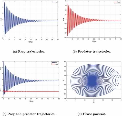
Table 1. Parameters values used for the numerical simulation of system (2)

Parameters	Values	References
$r_1$	1.0009	estimated
$r_2$	0.9000001	estimated
$K_1$	250	Savadogo et al. (2021) and Tewa et al. (2013)
$K_2$	90	Savadogo et al. (2021) and Tewa et al. (2013)
$k_1$	1.00089	estimated
$k_2$	0.00111594	estimated
$\omega$	0.08010099	estimated

Biologically, it means that the prey and the predator can survive in a long term together despite the predation. Thus, we talk about the phenomenon of subsistence.

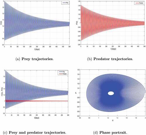
The parameters values used are always fixed in Table 1. By increasing the value $k_1$ to $k_1=1.8$, we observe a start of periodic behavior of the numbers of prey and predators, this is characterized by Figure (4(a–c)). The loss of stability of coexistence equilibrium $E_3$ are also observed on Figure (4(d)). This numerical experiment confirms the mathematical results established in Theorem 3.5 concerning local stability of coexistence equilibrium $E_3$.

Figure 4. Local asymptotic stability of the coexisting equilibrium of system (2) corresponding to $k_1=1.8$.

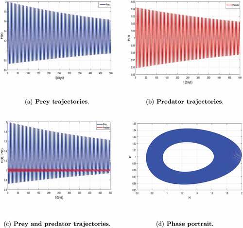
To examine the existence of limit cycles arising by Hopf bifurcation we increase the value of predation rate to $k_1=1.89$ and keeping the values of the other parameters fixed in Table 1. Thus, we observe a periodic behavior of system as indicated by (Figure (5a–c)). Figure (5(d)) shows that the coexistence equilibrium $E_3$ is unstable and we have a limit cycle arising from Hopf bifurcation. This is in accordance with the mathematical results established in Theorem 3.7. The biological interpretation is that the prey coexists with the predator, exhibiting oscillatory equilibrium behavior and this highlights an extinction of the population of prey (at risk) if predation rate exceeds a certain threshold.

Figure 5. Dynamics of the trajectories of model (2) with periodic solutions with $k_{1c}=1.89$.

Thus, we can conclude that predation is a key parameter which governs our model and is useful for understanding the dynamics prey-predator species in the ecosystem, and that it plays a regulator role of species.

4.2. Global behavior of system (5) with disease in the two populations

In this subsection, we present a series of numerical simulation to illustrate the theoretical findings obtained for model (5). Here the predation rate $k_1$, is an important parameter under investigation. The main goal of this subsection is to study the effect of predation on the disease transmission dynamics. To validate the analytical findings of the model, the parameter values used are given in Table 2. Figure 6(a–f) illustrate the existence and the global stability of the coexistence equilibrium $E_5(200;49.62;20;14)$ of the model (5). The parameter values which are chosen lead to $R_{02}=6.11>1$ and $R_{03}=1.33>1$, so the disease spreads among the preys and predators. This result is related to a similar threshold phenomenon in the study of epidemic models. Thus, the above results indicate that despite the persistence of disease, preys and predators can coexist. This numerical result confirms the mathematical results established in Theorem 3.10 concerning the persistence of the infection.

Figure 6. Global asymptotic stability of the coexisting equilibrium $E_5$ of model (5) when $R_{02}=6.11>1$ and $R_{03}=1.33>1$.

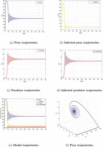
Table 2. Parameters values used for the numerical simulation of system (5)

Parameters	Values	References
$r_1$	1.8	Savadogo et al. (2021)
$r_2$	0.0123	estimated
$K_1$	350	estimated
$K_2$	100	estimated
$k_1$	1.01	estimated
$k_2$	0.0221	estimated
$\omega$	0.1	Savadogo et al. (2021) and Tewa et al. (2013)
${\beta }_1$	1.59	estimated
${\beta }_2$	1.59	estimated
${\sigma }_1$	0.15	Tewa et al. (2013)
${\sigma }_2$	0.15	Savadogo et al. (2021) and Tewa et al. (2013)
${\theta }_1$	0.89	estimated
${\theta }_2$	0.5	estimated
${\mu }_1$	0.05	estimated
${\mu }_2$	0.05	estimated
$\delta$	0.05	estimated

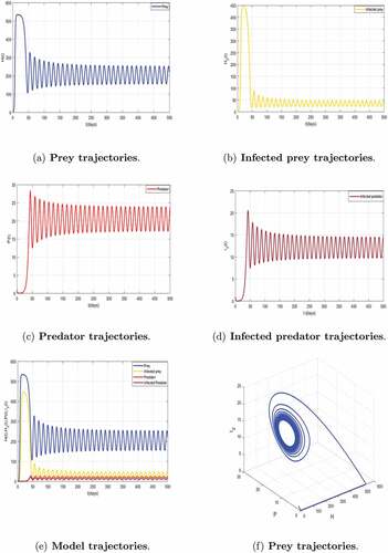
We continue our numerical investigation by increasing the value of $k_1$ to illustrate the behavior of the dynamics of system (5) and keeping fixed the values of the other parameters in Table 2. Indeed, for $k_1=1.1$ we observe an instability taking place for system (5) illustrated by Figure (7 (f)). We always have persistence of disease with $R_{03}=1.41>1.$ The local stability of system (5) around $E_4$ is illustrated by Figure (7(f)). This result supports Theorem 3.9.

Figure 7. Local asymptotic stability of the coexisting equilibrium $E_5$ of model (5) corresponding to $k_1=1.1$ with $R_{02}=6.11>1$, $R_{03}=1.41>1$.

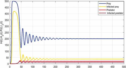
Finally, if we consider the critical value of predation rate to $k_1=k_{1c}=1.2$ and keeping fixed the other parameters in Table 2, a series of numerical simulations shows the increasing of ${\beta }_1,{\beta }_2$ to ${\beta }_1={\beta }_2=1.89$. The parameter values lead to $R_{03}=1.42>1.$ Figure 8(b,d) shows that the coexistence equilibrium $E_5$ is unstable, and we have a limited cycle arising from the Hopf bifurcation. Indeed, the limit cycle is a trajectory for which the dynamics of the system would be constant over a cycle. This means that the epidemic gets a limit progression.

Figure 8. Hopf-bifurcation of system (5) with persistence of disease in two populations population corresponding to $k_1=1.2$ with $R_{03}=1.42>1$.

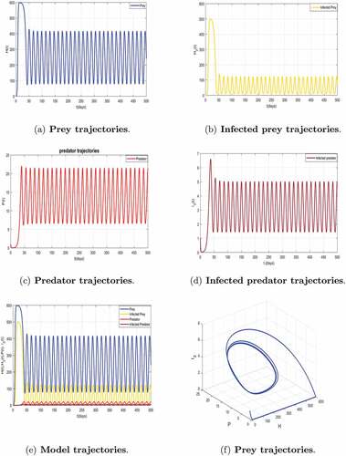
With regard to this observation, we can conclude that the predation rate is a key parameter that increases propagation of the disease in the dynamic of prey-predator model and destabilize the number of preys and predator. In order to avoid any extinction of the two species and the propagation of disease in nature, it is very important to control the predation phenomenon.

Thus, we can conclude that the predation rate is a key parameter that control the spreading of the disease in the dynamic of prey-predator model.

Remark 4.1. The biological interpretation of Hopf bifurcation is that predator coexists with the susceptible prey and the infected prey, exhibiting periodic balance behavior if the predation threshold $k_1>k_{1c}$. To avoid extinction of the species, one should look carefully some parameters, namely, the rate of predation, the rate of infection of the infective population and susceptible population.

5. Conclusion

The effect of predation on the transmission of infectious disease in a prey-predator models plays an important role in the propagation of diseases in the ecological system. It is in this point of view that in this paper, we have mainly proposed and analyzed a prey-predator model in the context of epidemic to describe the effect of the predation on the dynamic of transmission of an infectious diseases. We have incorporated Holling function response of type II to describe the predation strategy, because it determines the stability and bifurcation diagram of the model. To investigate the effect of predation in the transmission of disease in the prey-predator model, we subdivided our study in two parts.

Firstly, the prey-predator model without disease. The mathematical results obtained within the framework of this study allowed us first, to establish the positivity of the solutions indicating the existence of the population, as well as the bornitude to explain the natural control of the growth due to the restriction of the resources. Moreover, to ensures the long term survival of all populations (prey and predator), we established the uniform persistence of system (2). In addition, we established the conditions of existence of the coexistence equilibria. Under certain conditions of the predation rate, we established the local stability of the coexistence equilibrium. In order to show the long-term coexistence of prey and predator species, we established the global stability of the coexistence equilibrium via an appropriate Lyapunov function under certain conditions of the model parameters. Moreover, we have described the conditions of existence of Hopf bifurcation around coexistence equilibrium in order to highlight periodic variation of the number of prey and predator due to the effect of predation. In this subsection, we can conclude that preys or predators could go to extinction, could coexist or see their numbers vary periodically.

Secondly, we were interested in a prey-predator model with disease in the two populations. In the framework of this study we have assumed that the presence of infected preys is compensated by the presence of infected predators. However, according to Proposition 3.5 and Theorem 3.10, we remark that the presence of the disease in the two populations highlighted two news situations. Under certain conditions of predation rate, preys and predators population converge towards the equilibrium $E_3$ with disappearance of disease in the two populations $(R_{02}<1,R_{03}<1)$. And under certain other conditions of predation rate, prey and predator populations converge towards the coexistence equilibrium, but with persistence of the disease in the two populations $(R_{03}>1,R_{02}>1)$. Thus, we can conclude, that prey and predators can have numbers that vary periodically. This variation can occur with the disappearance of the disease in both populations, it can also occur with the persistence of the disease in predators first, then in two populations.

Finally, to support our analytical findings, numerical simulations have been done based on the formulas of section 3 to show the effect of predation on the disease transmission. We have showed numerically that for $k_1\in (1.01,1.2)$ an equilibrium is established with the coexistence of the populations. These numerical results are in agreement with the theoretical results in section 3. In addition, we observed that the disease persists in preys, or in predators and in the two populations $(R_{02}>1,R_{03}>1)$ with the increasing of the transmission rate from ${\beta }_1={\beta }_2=1.59$ to ${\beta }_1={\beta }_2=1.89$.

In the light of these observations, we can conclude that the predation rate is a key parameter which controls the propagation of the disease. To sustain the coexistence of ecosystem species and to avoid any extinction of the two species due to disease, it is very important to control predation parameter.

Our studies gives some new insights for understanding the dynamic of propagation of the diseases in the ecosystem and the information on biological networks, especially prey-predator models. Comparatively to (Tewa et al., 2013), we have extended the study proposed by establishing analytically the global stability of coexistence equilibrium when disease spread in two species. In order to take into account phenomenon of subsistence in the predators populations, we assumed that predators have an alternative source of food in introducing logistic growth in the predators population. That is more realistic in the ecosystem environment, because the food source of one predatory species does not depend exclusively on preys density.

In conclusion, we state that our model with disease in both predator and prey populations provide complex dynamics, allowing the possibility of bi-stability and periodic oscillation in the ecosystem. The existence of a coexistence equilibrium with predators and prey coexisting and both endemic is also biologically interesting, although we are not able to fully analyze it, especially analysis of Hopf bifurcation. Hence, is an appealing problem for our future studies.

Despite the important findings on this paper, in order to deepen our study, we plan to extend this work, taking into account the phenomenon of migration.

Disclosure statement

The authors declare that there are no conflicts of interest regarding the publication of this paper.

Additional information

Funding

The authors received no direct funding for this research.

Notes on contributors

Assane Savadogo

Assane Savadogo is a vigorous researcher PhD student at University Nazi Boni, currently in cotutelle at the prestigious Sorbonne University. His research interests lie in the field of Mathematical Modelling and the present paper is a portion of his thesis under the supervision of Prof. Boureima Sangaré.

Boureima Sangaré

Prof. Boureima Sangaré is working as a full professor at University Nazi Boni. His research interests lie in the field of Mathematical Biology; four PhD students obtained their PhD under his guidance and five PhD students are currently working with him. He has published his research contributions in different peer-reviewed and reputed internationally renowned journals whose publishers are Springer, Taylor & Francis, Elsevier, De Gruyter and other journals.

Hamidou Ouedraogo

Dr. Hamidou Ouedraogo is a former PhD student at University Nazi Boni under the supervision of Prof. Boureima Sangaré. A vigorous researcher in the area of Mathematical modelling, he has presented many papers in conferences and has nine research papers in reputed international journals.

References

- Akyildiz, F. T., & Alshammari, F. S. (2021). Complex mathematical SIR model for spreading of COVID-19 virus with Mittag-Leffler kernel. Advances in Difference Equations, 53(319), 1–22. https://doi.org/10.1186/s13662-021-03470-1
- Anderson, R. (1988). The epidemiology of HIV infection: Variable incubation plus infectious periods and heterogeneity in sexual activity. With discussion. Journal of the Royal Statistical Society. Series A (Statistics in Society), 151(1), 66–98. https://doi.org/10.2307/2982185
- Arditi, R., & Ginzburg, L. R. (1989). Coupling in predator-prey dynamics: Ratio-dependence. Journal of Theoretical Biology, 139(3), 311–326. https://doi.org/10.1016/S0022-5193(89)80211-5
- Bairagi, N., Roy, P., & Chattopadhyay, J. (2007). Role of infection on the stability of a predator-prey system with several response functions-a comparative study. Journal of Theoretical Biology, 248(1), 10–25. https://doi.org/10.1016/j.jtbi.2007.05.005
- Biswas, S., Samanta, S., & Chattopadhyay, J. (2018). A cannibalistic eco-epidemiological model with disease in predator population. Journal of Applied Mathematics and Computing, 57(1–2), 161–197. https://doi.org/10.1142/S0218127415501308
- Chiu, C. (1999). Lyapunov functions for the global stability of competing predators. Journal of Mathematical Analysis and Applications, 230(1), 232–241. https://doi.org/10.1006/jmaa.1998.6198
- Dimaschko, J., Shlyakhover, V., & Labluchanskyi, M. (2021). Why did the COVID-19 epidemic stop in China and does not stop in the rest of the world? (Application of the Two-Component Model). SciMed, 3(2), 88–99. https://doi.org/10.28991/SciMedJ-2021-0302-2
- Guin, L. N. (2014). Existence of spatial patterns in a predator-prey model with self- and cross-diffusion. Applied Mathematics and Computation, 226(2014), 320–335. https://doi.org/10.1016/j.amc.2013.10.005
- Hadeler, K., & Freedman, H. (1989). Predator-prey populations with parasitic infection. Journal of Mathematical Biology, 27(6), 609–631. https://doi.org/10.1007/BF00276947
- Haijiao, L., & Shangjiang, G. (2017). Dynamics of a SIRC epidemiological model. Electronic Journal of Differential Equations 2017 (121), 1–18.
- Haque, M., Ali, N., & Chakravarty, S. (2013). Study of a tri-trophic prey-dependent food chain model of interacting populations. Mathematical Biosciences, 246(1), 55–71. https://doi.org/10.1016/j.mbs.2013.07.021
- Haque, M., & Venturino, E. (2007). An eco-epidemiological model with disease in predator: The ratio-dependent case. Mathematical Methods in the Applied Sciences, 30(14), 1791–1809. https://doi.org/10.1002/mma.869
- Hethcote, H., Wang, W., Han, L., & Ma, Z. (2004). A predator-prey model with infected prey. Theoretical Population Biology, 66(3), 259–268. https://doi.org/10.1016/j.tpb.2004.06.010
- Hsieh, Y. H., & Hsiao, C. K. (2008). Predator-prey model with disease infection in both populations. Mathematical Medicine and Biology, 25(3), 247–266. https://doi.org/10.1093/imammb/dqn017
- Intissar, A. (2020). A mathematical study of a generalized SEIR model of COVID-19. SciMed, 2(2020), 30–67. https://doi.org/10.28991/SciMedJ-2020-02-SI-4
- Kermack, W., & McKendrick, A. (1927). A contribution to the mathematical theory of epidemics. Proceedings of the Royal Society of London, 115(772), 700–721. https://doi.org/10.1098/rspa.1927.0118
- Klempner, M. S., & Shapiro, D. S. (2004). Crossing the species barrier-one small step to man, one giant leap to mankind. New England Journal of Medicine, 12(350), 1171–1172. https://doi.org/10.1056/NEJMp048039
- Koutou, O., Traoré, B., & Sangaré, B. (2018a). Mathematical model of malaria transmission dynamics with distributed delay and a wide class of nonlinear incidence rates. Cogent Mathematics & Statistics, 5(25), 1564531. https://doi.org/10.1080/25742558.2018.1564531
- Koutou, O., Traoré, B., & Sangaré, B. (2018b). Mathematical modeling of malaria transmission global dynamics: Taking into account the immature stages of the vectors. Advances in Difference Equations, 2018(220), 34. https://doi.org/10.1186/s13662-018-1671–2
- Koutou, O., Traoré, B., & Sangaré, B. (2021). Analysis of schistosomiasis global dynamics with general incidence functions and two delays. International Journal of Applied and Computational Mathematics, 7(6), 245. https://doi.org/10.1007/s40819-021-01188-y
- Lotka, A. (1956). Elements of mathematical biology. Dover New York, 7(3), 145–214. https://doi.org/10.1002/jps.3030471044
- Mushanyu, J., Chazuka, Z., Mudzingwa, F., & Ogbogbo, C. (2021). Modelling the impact of detection on COVID-19 transmission dynamics in Ghana. Research in the Mathematical Sciences, 8(1), 1–11. https://doi.org/10.1080/27658449.2021.1953722
- Ouedraogo, H., Ouedraogo, W., & Sangaré, B. (2019). Bifurcation and stability analysis in complex cross-diffusion mathematical model of phytoplankton-fish dynamics. Journal of Partial Differential Equations, 8(3), 1–13. https://doi.org/10.4208/jpde.v32.n3.2
- Ouedraogo, H., Ouedraogo, W., & Sangaré, B. (2020). Cross and self-diffusion mathematical model with nonlinear functional response for plankton dynamics. Journal of Advanced Mathematical Studies, 13(2), 237–251.
- Rosenzweig, M. L., & MacArthur, R. (1963). Graphical representation and stability conditions of predator prey interactions. The American Naturalist, 97(895), 209–223. https://doi.org/10.1086/282272
- Sarwardi, S., Haque, M., & Venturino, E. (2011). A Leslie-Gower Holling-type II ecoepidemic model. Journal of Applied Mathematics and Computing, 35(1–2), 263–280. https://doi.org/10.1007/s12190-009-0355-1
- Savadogo, A., Ouedraogo, H., Sangaré, B., & Ouedraogo, W. (2020). Mathematical analysis of a fish-plankton eco-epidemiological system. Nonlinear Studies, 27(1), 1–22.
- Savadogo, A., Sangaré, B., & Ouedraogo, H. (2021). A mathematical analysis of Hopf-bifurcation in a prey-predator model with nonlinear functional response. Advances in Difference Equations, 400(275), 1–23. https://doi.org/10.1186/s13662-021-03437-2
- Subhas, K. (2017). Uniform persistence and global stability for a brain tumor and immune system interaction. Biophysical Reviews and Letters, 12(4), 1–22. https://doi.org/10.1142/S1793048017500114
- Tewa, J. J., Djeumen, V. Y., & Bowong, S. (2013). Predator–prey model with holling response function of type II and SIS infectious disease. Applied Mathematical Modelling, 37(7), 47–57. https://doi.org/10.1016/j.apm.2012.10.003
- Tozzi, A., & Peters, J. F. (2019). Topology of Black Holes’ Horizons. Emerging Science Journal, 3(2), 58. https://doi.org/10.28991/esj-2019-01169
- Traoré, B., Koutou, O., & Sangaré, B. (2019). Global dynamics of a seasonal mathematical model of schistosomiasis transmission with general incidence function. Journal of Biological Systems, 27(1), 19–49. https://doi.org/10.1142/S0218339019500025
- Traoré, B., Koutou, O., & Sangaré, B. (2020). A global mathematical model of malaria transmission dynamics with structured mosquito population and temperature variations. Nonlinear Analysis: Real World Applications, 53(2020), 1–33. https://doi.org/10.1016/j.nonrwa.2019.103081
- Traoré, B., Sangaré, B., & Traoré, S. (2018). A mathematical model of malaria transmission in a periodic environment. Journal of Biological Dynamics, 12(1), 400–432. https://doi.org/10.1080/17513758.2018.1468935
- Vidyasagar, M. (1980). Decomposition techniques for large-scale systems with nonadditive interactions: Stability and stabilizability. IEEE Transactions on Automatic Control, 25(4), 773–779. https://doi.org/10.1109/TAC.1980.1102422
- Xia, Y., Lansun, C., & Jufan, C. (1996). Permanence and positive periodic solution for the single-species nonautonomous delay diffusive models. Computers & Mathematics with Applications, 32(4), 109–116. https://doi.org/10.1016/0898-1221(96)00129-0
- Xiao, Y., & Chen, L. (2001). Modeling and analysis of a predator-prey model with disease in the prey. Mathematical Biosciences, 171(1), 59–82. https://doi.org/10.1016/s0025-5564(01)00049-9
- Xiaolei, Z., Renjun, M., & Lin, W. (2020). Predicting turning point, duration and attack rate of COVID-19 outbreaks in major Western countries. Chaos, Solitons & Fractals, 135(2020). https://doi.org/10.1016/j.chaos.2020.109829
- Zhan, S., Shuyuan, Q., Jinfang, Y., Jianwei, Z., Sisi, S., Long, T., Jun, L., Linqi, Z., Wang, W. (2021). Bat and pangolin coronavirus spike glycoprotein structures provide insights into SARS-CoV-2 evolution. Nature Communications, 12(1607), 1–12. https://doi.org/10.1038/s41467-021–21767-3.