A Novel Minimization Approximation Cost Classification Method to Minimize Misclassification Rate for Dichotomous and Homogeneous Classes

ABSTRACT

Dependence of the linear discriminant analysis on location and scale weakens its performance when predicting class under the presence of homogeneous covariance matrices for the candidate classes. Further, outlying samples render the method to suffer from higher rates of misclassification. In this study, we propose the minimization approximation cost classification (MACC) method that accounts for some specific cost function $23.9$. The theoretical derivation is made to find an optimal linear hyperplane $\theta$, which yields maximum separation between the dichotomous groups. Real-life data and simulations were used to validate the method against the standard classifiers. Results show that the proposed method is more efficient and outperforms the standard methods when the data are crowded at the class boundaries.

KEYWORDS:

• Linear discriminant analysis
• majorization-minimization principle
• misclassification rate
• minimization approximation cost function
• optimal linear hyperplane

1. Introduction

The idea to optimize the cost function has been of interest since the second half of twentieth century (Gibra, 1967). For instance, engineers in a factory may need to control and optimize the total production cost of goods associated with high quantity and quality in a short time (Zavvar Sabegh et al., 2016). Minimizing the cost is important and has several applications. For example, in the health sector, the risk of misclassifying an infected person with a very contagious disease such as COVID-19 and influenza can be disastrous as many more people could get infected. Researchers in health science may need to minimize the cost of misclassifying patients, especially as they allocate them to wards so as to minimize the undesired outcomes.

Models have been used in medicine and engineering to predict the class membership such as multilevel logistic model (Dey & Raheem, 2016). However, classification when data are crowded around the separable hyperplane still remains a major statistical research problem. The popularly used standard linear discriminant analysis as well as the quadratic discriminant analysis are often characterized with high misclassification rates(Young, D. M.,Raudys,2004). The dependence of these methods on location and covariance weakens their class prediction performance under the assumption of homogeneity of the covariance matrix.

Besides, presence of outlying samples may also render these methods amenable to high misclassification rates. Therefore, the major contribution of our study was to develop suitable cost function that can be used in the classification problem so as to minimize misclassification rates.

1.1. Defining the classification problem

The multivariate classification problem involves grouping the features ${\mathbf{X}}_{\mathbf{i}}$ in ${\mathbf{R}}^{\mathbf{p}}$ space to one of the group membership $y_i\in R$. The general form of linear classification function for the binary outcomes $y_i=sign\left\{f({\mathbf{X}}_{\mathbf{i}})\right\}$ where $y_i\in \left\{-1,1\right\}$ and $f({\mathbf{X}}_{\mathbf{i}})={\theta }^T{X}_{i}i=1,2,3,\dots .,N.$ The linear discriminant analysis (LDA), sometimes called the Fisher’s approach, is the most basic linear classifier. As indicated in other studies, this method does not require to satisfy the normality assumption (Liong & Foo, 2013; Tillmanns & Krafft, 2017). Its main assumption is homogeneity of the group covariance matrices, as is the case for the two-group classification (Puntanen, 2013). The general idea of the LDA is to construct a linear hyperplane so as to separate the two groups as much as possible. Suppose we have a random variable ${\mathbf{X}}_{\mathbf{i}},(i=1,2,\dots ,N)$ from one of the two groups ${\mathbf{y}}_{\mathbf{i}}\in \{-1,1\}$ with ${\mathbf{X}}_{\mathbf{1}}\sim \varphi ({\mu }_{\mathbf{1}},{\mathrm{\Sigma }}_{\mathbf{1}})$ and ${\mathbf{X}}_{\mathbf{2}}\sim \varphi ({\mu }_{\mathbf{2}},{\mathrm{\Sigma }}_{\mathbf{2}})$, where $\varphi$ is any multivariate distribution, which is not necessarily the normal distribution. We wish to classify each data vector ${\mathbf{X}}_{\mathbf{i}}$ of size $p\times 1$ to the binary group membership $\{-1,+1\}$ where the number of groups $k=2$. The overall covariance matrix is indicated by: ${\sum }_{\mathbf{X}}$ such that ${\mathrm{\Sigma }}_{\mathbf{X}}={\mathrm{\Sigma }}_{\mathbf{B}}+{\mathrm{\Sigma }}_{\mathbf{W}}$, where:

${\mathrm{\Sigma }}_{\mathbf{X}}=\sum _{\mathbf{j}\mathbf{=}\mathbf{1}}^{\mathbf{2}}\sum _{\mathbf{i}\mathbf{=}\mathbf{1}}^{\mathbf{N}}\left({\mathbf{X}}_{\mathbf{i}\mathbf{j}}-\mu \right){\left({\mathbf{X}}_{\mathbf{i}}-\mu \right)}^{\mathbf{T}},{\mathrm{\Sigma }}_{\mathbf{B}}=\mathbf{N}\sum _{\mathbf{j}\mathbf{=}\mathbf{1}}^{\mathbf{2}}\left({\mu }_{\mathbf{j}}-\mu \right){\left({\mu }_{\mathbf{j}}-\mu \right)}^{\mathbf{T}}$

and

${\mathrm{\Sigma }}_{\mathbf{W}}=\sum _{\mathbf{j}\mathbf{=}\mathbf{1}}^{\mathbf{2}}\sum _{\mathbf{i}\mathbf{=}\mathbf{1}}^{{\mathbf{N}}_{\mathbf{j}}}\left({\mathbf{X}}_{\mathbf{i}\mathbf{j}}-{\mu }_{\mathbf{j}}\right){\left({\mathbf{X}}_{\mathbf{i}\mathbf{j}}-{\mu }_{\mathbf{j}}\right)}^{\mathbf{T}}$

where: ${\mathrm{\Sigma }}_B$ and ${\mathrm{\Sigma }}_W$ are the between and within class covariance matrices. The data vector $X_{ij}$ in the $j^{th}$ with ${\mu }_j$ being its true mean vector for the $j^{th}$ class, while $\mu$ is the overall true mean vector.

The theoretical mechanism of finding the optimal linear separable hyperplane is estimating the parameter $\theta$ that maximizes data variation between the classes and minimizes the variations within each class. In other words, it is equivalent to maximizing the standardized squared distance from their centroids:

(1) $\frac{{\theta }^T{\mathrm{\Sigma }}_B\theta }{{\theta }^T{\mathrm{\Sigma }}_W\theta }\approx \frac{{\left({\bar{z}}_1-{\bar{z}}_2\right)}^2}{{\sigma }_z^2}=\frac{{\left[{\theta }^T\left({\mu }_1-{\mu }_2\right)\right]}^2}{{\theta }^T{\mathrm{\Sigma }}_p\theta }$(1)

where ${\bar{z}}_j$ is the transformed data vector that belongs to the $j^{th}\mathrm{\forall }j=1,2$ classes. The parameter for the linear hyperplane is $\theta$ while ${\sigma }_z^2$ is the variance for the transformed values of $z_i={\theta }^T{X}_i,i=1,\dots ,N$ and ${\mathrm{\Sigma }}_p$ is the pooled covariance matrix of $X$

Consequently, the middle part of the expression in Equation [1](1) $\frac{{\theta }^T{\mathrm{\Sigma }}_B\theta }{{\theta }^T{\mathrm{\Sigma }}_W\theta }\approx \frac{{\left({\bar{z}}_1-{\bar{z}}_2\right)}^2}{{\sigma }_z^2}=\frac{{\left[{\theta }^T\left({\mu }_1-{\mu }_2\right)\right]}^2}{{\theta }^T{\mathrm{\Sigma }}_p\theta }$(1) can be shown to be equivalent to the right hand part, by assuming that the parent populations have different population means but equal variances. Thereby, one unbiased estimator of population variance ${\sigma }_Z^2$ is the combined variance: $\frac{(n_1-1)s_{z_1}^2+(n_2-1)s_{z_2}^2}{(n_1+n_2-2)}$, where $s_{z_1}^2$,$s_{z_2}^2$ are the sample variances for the transformed values of class 1 and class 2 respectively.

The idea of Fisher’s approach in binary classification is to find a vector (${\theta }_{\mathbf{p}\times \mathbf{1}}$) that maximizes the standardized squared distance between the two centroid groups. The algebraic representation for this idea is in the following maximization problem:

$\underset{\theta }{max}\frac{{\left({\bar{z}}_1-{\bar{z}}_2\right)}^2}{{\sigma }_z^2}subjectto:{\bar{z}}_j={\theta }^T{\mu }_j$

where, ${\sigma }_z$ is the standard deviation for all N data vectors. By having sufficient samples $n=n_1+n_2$ from both population groups $N_1+N_2=N$, it can be assumed that our populations are normally distributed. Hence, the maximum likelihood estimators for the overall mean vector $\mu$ and $\mathrm{\Sigma }$, that is, $\bar{\mathbf{X}}$ and $\mathbf{S}$ respectively, can be used. By using these estimators, $\bar{\mathbf{X}}$ and $\mathbf{S}$, we can show the following:

$\frac{{\left({\bar{z}}_1-{\bar{z}}_2\right)}^2}{s_z^2}=\frac{{\left[{\theta }^T\left({\bar{X}}_1-{\bar{X}}_2\right)\right]}^2}{{\sum }_{i=1}^n{\left(z_i-\bar{z}\right)}^2}<\frac{{\theta }^T{S}_B\theta }{{\theta }^T{S}_W\theta };since{S}_X=S_B+S_W$

The right hand side of the last inequality is the Fisher-Roa’s Criterion, where $S_B$ is the between-class sample covariance matrix, $S_X$ is the total-class sample covariance matrix and $S_W$ is the within-class sample covariance matrix, and all these estimates are the maximum likelihood estimators. Hence, maximizing the standardized squared distance between groups involves minimizing the within group-sample covariance matrices.

The lemma by Johnson and Wichern (Puntanen, 2013) who used the extended Cauchy-Schwarz inequality for optimization was adopted in our search for an optimal estimate of $\theta$ in Equation (1)(1) $\frac{{\theta }^T{\mathrm{\Sigma }}_B\theta }{{\theta }^T{\mathrm{\Sigma }}_W\theta }\approx \frac{{\left({\bar{z}}_1-{\bar{z}}_2\right)}^2}{{\sigma }_z^2}=\frac{{\left[{\theta }^T\left({\mu }_1-{\mu }_2\right)\right]}^2}{{\theta }^T{\mathrm{\Sigma }}_p\theta }$(1) .

Lemma 1.1. Let ${\mathbf{B}}_{\mathbf{p}\times \mathbf{p}}$ be a symmetric positive definite matrix and ${\mathbf{d}}_{\mathbf{p}\times \mathbf{1}}$ be a given vector. Then for any arbitrary nonzero vector ${\mathbf{x}}_{\mathbf{p}\times \mathbf{1}}$,

(2) $ma{x}_{x\ne 0}\frac{{\left({\mathbf{x}}^{\mathbf{T}}\mathbf{d}\right)}^2}{{\mathbf{x}}^{\mathbf{T}}\mathbf{B}\mathbf{x}}={\mathbf{d}}^{\mathbf{T}}\hspace{0.17em}{\mathbf{B}}^{\mathbf{-}\mathbf{1}}\mathbf{d}$(2)

attained at $\mathbf{x}=c{\mathbf{B}}^{\mathbf{-}\mathbf{1}}\mathbf{d}$ for any scalar $c\ne 0$.

After matching the vector $x$ with the right hand side of Equation (1)(1) $\frac{{\theta }^T{\mathrm{\Sigma }}_B\theta }{{\theta }^T{\mathrm{\Sigma }}_W\theta }\approx \frac{{\left({\bar{z}}_1-{\bar{z}}_2\right)}^2}{{\sigma }_z^2}=\frac{{\left[{\theta }^T\left({\mu }_1-{\mu }_2\right)\right]}^2}{{\theta }^T{\mathrm{\Sigma }}_p\theta }$(1) , we found that $\mathbf{B}\mathbf{=}{\mathbf{S}}_{\mathbf{p}}$ and $\mathbf{d}\mathbf{=}{\bar{\mathbf{x}}}_{\mathbf{1}}\mathbf{-}{\bar{\mathbf{x}}}_{\mathbf{2}}$. Taking into account a normalized vector x gives c = 1.

The new version of this estimated hyperplane resulted by an iterative method that tries to minimize the covariance within each group ${\mathbf{S}}_{\mathbf{w}}$. We used the cost function $C(\theta )$ to minimize the data points from their corresponding centroids and consequently minimized the denominator containing ${\mathbf{S}}_{\mathbf{w}}$.

1.2. A motivating example

The search for another method that minimizes the misclassification between groups has been motivated by a number of studies (Croux & Joossens, 2005; Shen et al., 2011; Velilla & Hernndez, 2005; Zhang, 2004). Further motivation was from our exploratory analysis of simulation results from different distributions of data that revealed the effect of dispersion on the MCR. It was observed that as more data concentrate around boundary (separable hyperplane), their separation becomes very difficult as seen in Figures 1, 2. There are many data points close to the linear separable hyperplane such as the points; 10, 17, 34 and 56 from the squares group, which are highly likely to be misclassified. In other words, the risk of losing the information in estimating the optimal hyperplane is expected to be higher for the points around the hyperplane than the other points in the same group, where $\mathbf{R}({\mathbf{x}}_{\mathbf{i}})=\mathbf{E}[\mathbf{L}({\mathbf{x}}_{\mathbf{i}})]$ (Mengyi et al., 2012).

Figure 1. Distribution of simulated binary-class data to demonstrate the misclassification problem.

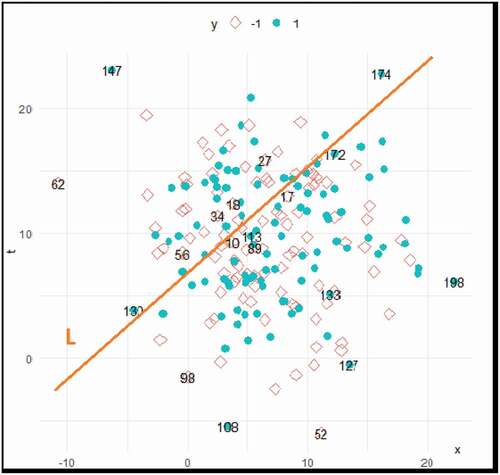
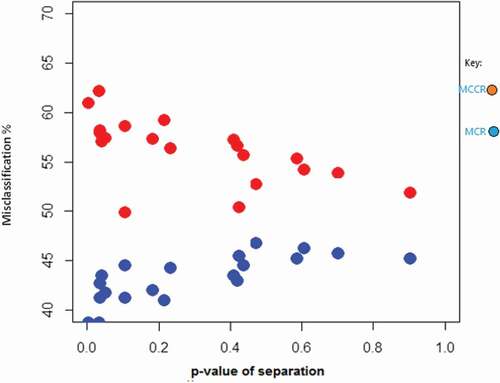
Figure 2. Relationship between p-value separation and misclassification.

Moreover, among the circular points, there are also data points such as 113,172 and 174 which are highly likely to be misclassified. It is logical, therefore, that fixing the same cost of misclassification for all data points is unfair. This leads to our idea that introducing a suitable cost function using the MM-principle(Mairal, 2013; Shen et al., 2011; Wang & Zou, 2018) would vary the cost for each data value according to how far this data point locates from the class mean vector. Hence, we will refer to the misclassification rate for the new method as minimal cost classification rate (MCCR), while the new method will be referred to as approximation minimization cost classifier (AMCC).

Thus, the aim of our study was to develop an optimal separable linear hyperplane using the MM-principle with cost function (discussed in section 2) that minimizes the rate of misclassification MCR. Also, in the next section we show how the algorithm to obtain the updated separable hyperplane that depends on the current one was derived. In section 3, we validate the proposed method by simulating some datasets and comparing them with the classical approaches in terms of misclassification rate. Further, real life datasets were used to further assess the proposed method by utilizing various train-test methods such as; SLDA, BSM, LOOCV and KFCV. All these train-test techniques are discussed in details in section 4. Ultimately, simulated dataset were used to discover the asymptotic behaviour of the proposed method and MCCR comparison to the MCR of SLDA.

2. Methodology

2.1. Developing the MACC based on the loss function

To achieve the study objectives, we applied a loss function to map values of one or more observed variables onto a real number representing some “cost” associated with the training item in the data (Shen et al., 2011). The total information lost can be represented by the cost function. In fact, the history of minimizing the MCR by using the loss function is a motivation to many researchers, for example, those who have worked to obtain optimum estimators of precision matrix ${\mathrm{\Sigma }}^{-1}$ under quadratic loss function (Mengyi et al., 2012). Cost may be taken as the average of the losses. We explored a quadratic loss function represented by $({\mathbf{x}}_{\mathbf{i}}-{\hat{\mu }}_{\mathbf{i}})$ where ${\hat{\mu }}_i$ is the expected value of ${\mathbf{x}}_{\mathbf{i}}$. It measures how much information is lost between the observed and its predicted value for each data item. A specific form of this cost function is the mean square error abbreviated by MSE.

$MSE=\sum _{i=1}^n\frac{{(x_i-{\hat{\mu }}_i)}^2}{n}$

where the ${\hat{\mu }}_i$ is the corresponding expected value of $x_i$. In this study we used the quadratic loss function. Therefore, for the linear discriminant analysis (LDA), our cost function is:

(3) $C_j(z_i)=\sum _{i=1}^n(z_{ij}-{\bar{z}}_j{)}^{2}wherej=1,2,...K$(3)

$z_{ij}$: the transformed value of the vector item $X_j$ in the $j^{th}$ group.

${\bar{z}}_j$: the transformed value of the mean vector of the $j^{t}h$ group.

The reason for choosing quadratic cost function was for its ease to show that the total cost for both groups in terms of hyperplane $\theta$ can be written as: $C(\theta )={\theta }^T({\mathrm{\Sigma }}_1+{\mathrm{\Sigma }}_2)\theta$. Therefore, minimizing the total cost requires minimizing the within-class variance for both groups by choosing the optimal value of $\theta$. Thus, this mechanism is similar to the approach of the Fisher-Roa’s Criterion which attempts to project the data points towards the centres of the groups, especially when many data points are concentrated around the marginal boundaries (Ahn & Marron, 2010). In some studies this process is called the data piling method which is projecting the high-dimensional data $(p>n)$ into the low dimension leading to maximizing the marginal distance between groups and projecting the data values that are concentrated on the boundaries towards the centres of groups. On the other hand, our proposed method tries to vary the cost needed to minimize based on the location of the data points from their class centres. The main difference is that in data piling, a kernel trick is used, whereas in our method we use the cost function. Therefore, our method works in parallel with classifiers, making it easy to validate against the classical methods of classification.

2.2. Overview of the Proposed MACC Method

We applied the majorization-minimization (MM) principle to find an expression that solves the iteratively updated separable hyperplane $\theta$ in terms of the current solution $\tilde{\theta }$ such that $\theta =f(\tilde{\theta })$. After some iterations, the updated $\theta$ gives an optimum such that the total cost $C(\theta )$ is at minimum. One limitation is how to obtain an optimum single closed form of $\theta$ from the direct differentiation of the cost function $C(\theta )$. However, a mechanism of direct differentiation does not always lead to a closed form of $\theta$ neither does it produce right desired solution. It can be shown that expressing cost function (7) in terms of $\theta$ and differentiating partially yields $\theta =\mathbf{0}$ which is logically impossible. Generally, the MM-principle operates in two steps. The first step searches for the majorization function $\mathbf{D}(\theta |\tilde{\theta })$ such that $\mathbf{C}(\theta )\le \mathbf{D}(\theta |{\theta }_k)$ for any $\theta \ne {\theta }_k$ The second step involves differentiating the $\mathbf{D}(\theta |{\theta }_k)$ with respect to $\theta$ and setting it to $0$ and iteratively finding an expression that involves $\theta$ and $\hat{\theta }$ (Lange & TongWu, 2008; Wang & Zou, 2018). In fact, based on Fisher’s approach (Shin, 2008), $\theta$ takes the form of $\theta =({\beta }_1,{\beta }_2,\dots ,{\beta }_p{)}^T$ for $p$ predictors. Finding the convex supremum majorization function $\mathbf{D}(\theta |\tilde{\theta })$ for any $\theta \ne \tilde{\theta }$ is quite difficult. By doing some manipulation using this principle, it can be called approximation-minimization principle. This can be reached algebraically using quadratic convex approximated function of the cost function (3), such that for any $\theta \ne \tilde{\theta }$, the function:

(4) $f(h(\theta ))\approx f(h(\tilde{\theta }))+f^{\prime }(h(\tilde{\theta }))(h(\theta )-h(\tilde{\theta }))+f(h(\tilde{\theta }))2!{(h(\theta )-h(\tilde{\theta }))}^2$(4)

where $f(.)$ is the cost function and $h(\theta )$ is the corresponding value of the linear classification function with unknown parameter $\theta$. Note that the right hand side of this inequality is approximated by the Taylor series approximation (Wu et al., 2019). In addition, $\tilde{\theta }=({\tilde{\beta }}_1,\dots ,{\tilde{\beta }}_p{)}_{p\times 1}^T$ is the current solution and $\theta =({\beta }_1,{\beta }_2,\dots ,{\beta }_p{)}^T$ is the updated solution (Mairal, 2013; Wang & Zou, 2018).

2.3. Deriving the minimization maximization cost classification (MACC)

Given the data matrix ${\mathbf{X}}_{\mathbf{n}\times \mathbf{p}}$ with the $i^{th}$ row $x_i^T$. Let $\tilde{\mathbf{b}}$ be an $n\times 1$ vector with the $i^{th}$ element $f^{\prime }({\tilde{\theta }}^T{x}_i)$, $\tilde{\theta }$ be the current solution and $\theta$ the updated solution, then $y_i=sign\left\{{\theta }^{\mathbf{T}}{\mathbf{x}}_{\mathbf{i}}\right\}$ is the linear classification function.

$C(\theta )=\sum _{i=1}^{n}f({\theta }^T{x}_i)\approx \mathbf{D}(\theta |\tilde{\theta })$

$=\sum _{i=1}^{n}f({\tilde{\theta }}^T{x}_i)+\sum _{i=1}^n{f}^{\prime }({\tilde{\theta }}^T{x}_i)({\theta }^T{x}_i-{\tilde{\theta }}^T{x}_i)+$

$\sum i=1nf(\theta T{x}_i)2{({\theta }^T{x}_i-\theta T{x}_i)}^2$

$=\sum _{i=1}^{n}f(({\tilde{\theta }}^T{x}_i)+$

$\sum _{i=1}^n{f}^{\prime }({\tilde{\theta }}^T{x}_i)\left[{\theta }^T{x}_i\right]+\sum _{i=1}^n{f}^{\prime }({\tilde{\theta }}^T{x}_i)\left[{\tilde{\theta }}^T{x}_i\right]$

$+\frac{1}{2}{\displaystyle \sum _{i=1}^{n}f}(\theta T{x}_i){\theta }^T{x}_i-\theta T{x}_{i}2$

Since $f(\theta T{x}_i)=2$ for any $x_i$ and $\mathrm{\forall }\theta$, then

$\mathbf{D}(\theta |\tilde{\theta })=\sum _{i=1}^{n}f({\tilde{\theta }}^T{x}_i)+\sum _{i=1}^n{\tilde{b}}_i{\theta }^T{x}_i-\sum _{i=1}^n{\tilde{b}}_i{\tilde{\theta }}^T{x}_i+\sum _{i=1}^n({\theta }^T{x}_i{)}^2+\sum _{i=1}^n({\tilde{\theta }}^T{x}_i{)}^2-2\sum _{i=1}^n\left\{{\theta }^T{x}_i{x}_i^T\tilde{\theta }\right\}$

$=\sum _{i=1}^{n}f({\tilde{\theta }}^T{x}_i)+{\theta }^T\sum _{i=1}^n{x}_i-{\tilde{\theta }}^T\sum _{i=1}^n{\tilde{b}}_i{x}_i+\sum _{i=1}^n({\theta }^T{x}_i{)}^2+\sum _{i=1}^n({\tilde{\theta }}^T{x}_i{)}^2$

$-2\left\{{\theta }^T\sum _{i=1}^n(x_i{x}_i^T)\tilde{\theta }\right\}$

$=\sum _{i=1}^{n}f({\tilde{\theta }}^T{x}_i)+{\theta }^T{X}^T\tilde{b}-{\tilde{\theta }}^T{X}^T\tilde{b}+\sum _{i=1}^n({\theta }^T{x}_i{)}^2+\sum _{i=1}^n({\tilde{\theta }}^T{x}_i{)}^2-2\left\{{\theta }^T\sum _{i=1}^n(x_i{x}_i^T)\tilde{\theta }\right\}$

$\equiv \mathbf{D}(\theta |\tilde{\theta })$

Now in order to find the iterative equation of $\theta$ in terms of $\hat{\theta }$, we differentiate the majorization (approximation) function $\mathbf{D}(\theta |\tilde{\theta })$ with respect to ${\theta }^{\mathbf{T}}$, and set it equal to ${\mathbf{0}}_{\mathbf{p}\times \mathbf{1}}$ as follows:

(5) $\frac{\mathrm{\partial }D}{\mathrm{\partial }{\theta }^T}=0+{\tilde{b}}^{T}X-0+2{\theta }^T\sum _{i=1}^n(x_i{x}_i^T)+0-2{\tilde{\theta }}^T{\left(\sum _{i=1}^n(x_i{x}_i^T)\right)}^T=0.$(5)

Solving Equation (5)(5) $\frac{\mathrm{\partial }D}{\mathrm{\partial }{\theta }^T}=0+{\tilde{b}}^{T}X-0+2{\theta }^T\sum _{i=1}^n(x_i{x}_i^T)+0-2{\tilde{\theta }}^T{\left(\sum _{i=1}^n(x_i{x}_i^T)\right)}^T=0.$(5) for ${\theta }^T$ gives (Equation 6(6) ${\theta }^T={\tilde{\theta }}^T-\frac{1}{2}{\tilde{b}}^{T}X{\left(\sum _{i=1}^n{x}_i{x}_i^T\right)}^{-1}.$(6) ):

(6) ${\theta }^T={\tilde{\theta }}^T-\frac{1}{2}{\tilde{b}}^{T}X{\left(\sum _{i=1}^n{x}_i{x}_i^T\right)}^{-1}.$(6)

The Equation (6)(6) ${\theta }^T={\tilde{\theta }}^T-\frac{1}{2}{\tilde{b}}^{T}X{\left(\sum _{i=1}^n{x}_i{x}_i^T\right)}^{-1}.$(6) can be iterated a number of times to get an updated solution $\theta$ (the hyperplane) until a desired minimum misclassification rate is reached. A threshold $\text{isin}>0$ is the desired minimum misclassification rate that can be set by the researcher. It can also be defined as $\parallel \theta -\hat{\theta }{\parallel }_2$ where $\theta$ is the updated solution and $\hat{\theta }$ the previous solution. Moreover, if the issue of over fitting arises, it can be solved through the cross-validation method. In Algorithm (1) we show how the estimated value of $\theta$ can be iteratively determined such that the rate of misclassification MCR does not exceed $\text{isin}.$ However, the proposed method performs well under the assumptions of homogeneity of groups and the nonsingularity of the matrix ${\sum }_{i=1}^n\left(x_i{x}_i^T\right)$. Also using the Taylor’s approximation in the majorization function, and putting the parameter $\theta$ in the explicit form of the Fisher’s approach: $\theta =({\mu }_1-{\mu }_2{)}^{T}A$ gives one property of this majorization function $\mathbf{D}(\theta |\tilde{\theta })$ based on its partial derivatives with respect to the two mean vectors.

Further, we let $\theta =({\mu }_1-{\mu }_2{)}^{T}A$ in our majorization function $D(\theta |\tilde{\theta })$ and taking partial with respect to ${\mu }_1$ and ${\mu }_2$, to get expressions in Equations (7)(7) $\frac{\mathrm{\partial }D}{\mathrm{\partial }{\mu }_1}=0+Z^{T}YA-0+2\sum _{i=1}^n({\mu }_1-{\mu }_2{)}^{T}A{y}_i(A{y}_i{)}^T+0-2({\mu }_1^{\sim }-{\mu }_2^{\sim }{)}^T{A}^{\sim }\sum _{i=1}^n(y_i{y}_i^T)A^T=0$(7) and (12) respectively:

(7) $\frac{\mathrm{\partial }D}{\mathrm{\partial }{\mu }_1}=0+Z^{T}YA-0+2\sum _{i=1}^n({\mu }_1-{\mu }_2{)}^{T}A{y}_i(A{y}_i{)}^T+0-2({\mu }_1^{\sim }-{\mu }_2^{\sim }{)}^T{A}^{\sim }\sum _{i=1}^n(y_i{y}_i^T)A^T=0$(7)

(8) $\frac{\mathrm{\partial }D}{\mathrm{\partial }{\mu }_2}=0-Z^{T}YA+0-2\sum _{i=1}^n({\mu }_1-{\mu }_2{)}^{T}A{y}_i(A{y}_i{)}^T-0+2({\mu }_1^{\sim }-{\mu }_2^{\sim }{)}^T{A}^{\sim }\sum _{i=1}^n(y_i{y}_i^T)A^T=0$(8)

consequently:

(9) $\frac{\mathrm{\partial }D}{\mathrm{\partial }{\mu }_1}+\frac{\mathrm{\partial }D}{\mathrm{\partial }{\mu }_2}=0$(9)

The last partial differential equation implies that in order to minimize the majorization function $D(\theta )$ and consequently minimize the cost function $C(\theta )$, leads to minimum misclassification rate $MCR$. Note that the rate of change of $D(\theta )$ with respect to ${\mu }_1$ should be approximately the same rate change of $D(\theta )$ with respect to ${\mu }_2$ but in the opposite direction, while preserving homogeneity within groups.

2.4. A Pseudocode for the updated MACC hyperplane$\theta$

To illustrate the application of the proposed minimal cost classification rate (MCCR), the pseudocode in algorithm (1) describes the procedure for updating the hyperplane $\theta$. It is necessary to set the desired misclassification rate $\text{isin}$, sample size, $n$ and number of iteration,iter that represent the maximum number of iterations required to update the hyperplane $\theta$. Then, the parameters $\alpha$ and $\beta$ are set to be positive so as to control the variances in the covariance matrices $\alpha I$ and $\beta I$, where $\mathbf{I}$ is an identity matrix. We then, simulate $n/2$ samples for each group and estimate the covariance matrix and population mean $(\sum ,\mu )$ for both groups from previous samples. If real data set is available, simulation part may not be required. After which, we suggest conducting a test for homogeneity between groups $H_0:{\sum }_1={\sum }_2$ as well as their separation $H_0:{\mu }_1={\mu }_2$ to ascertain meaningful classification and separation required for using this method. Finally, we update $\theta$ at each iterative step $\tau$ by using Equation (6)(6) ${\theta }^T={\tilde{\theta }}^T-\frac{1}{2}{\tilde{b}}^{T}X{\left(\sum _{i=1}^n{x}_i{x}_i^T\right)}^{-1}.$(6) to find the minimum misclassification rate (MCCR) that corresponds to the optimum $\theta$.

Algorithm 1: The Pseudo code to implement Minimal Cost Function based on LDA

Data: file.txt

Result: calculate the MCCR

Test ${\mu }_1={\mu }_2\text{amp}{\sum }_1={\sum }_2$;

initialization $\theta ,\hspace{0.17em}iter\hspace{0.17em},\text{isin}>0,\tau =1$;

while $\tau <iter$ do

Calculate $z_i=\theta x_i$;

Find the Lost information of $z_i$ using Quadratic cost;

Update $\theta$ using Equation 6(6) ${\theta }^T={\tilde{\theta }}^T-\frac{1}{2}{\tilde{b}}^{T}X{\left(\sum _{i=1}^n{x}_i{x}_i^T\right)}^{-1}.$(6) ;

Calculate MCR;

if MCR $>\text{isin}$ then

$\tau \leftarrow \tau +1;$

current $\theta$ is updated;

else

MCCR $\leftarrow$ MCR;

Exit;

end

end

3. Validation of the proposed MACC method by monitoring the MCCR

The efficiency of our method is validated by comparing its misclassification rate, MCCR against that from four different classification methods, including; the standard linear discriminant analysis SLDA, bootstrapping sampling method BSM, leave-one-out-cross-validation LOOCV and the k-fold cross-validation KFCV. We compare them by assessing their performance based on their resulting misclassification rates MCR. Here is a brief description for each method:

(1) The SLDA is the Fisher’s approach for classification (Puntanen, 2013; Shin, 2008).

(2) In the BSM, some samples are selected randomly from the dataset with specific sample sizes, fitting the linear model that leads to predict the group’s memberships for the remaining unselected samples and consequently compute the MCR. This process was repeated many times and finally the average MCR is calculated (Shao, 1993).

(3) The LOOCV splits the data set into two parts; the “train”, a frame that contains all samples except one data subject and the “test” frame. Train set is used to fit the linear classifier which takes the one left subject to predict its corresponding group membership. This process was continued until all subjects in the dataframe were completed giving the final result for the MCR (Xu & Goodacre, 2018).

(4) Under the KFCV, the data is divided the data into k-parts, which should contain relatively equal subjects. It is an extension for the LOOCV, but the test set contains more than one subject. At each time, one fold was treated as test frame and the others used to fit the model. At the end, we averaged the $k$ MCRs (Xu & Goodacre, 2018).

(5) MCCR is the misclassification rate calculated from the new proposed method that uses the cost function based on the MM-principle.

3.1. Validation of the MACC method using simulation study

Datasets of different sizes $N$ with $N/2$ data values in each each group and seven predictors $p=7$ were generated from two multivariate normal distributions with known parameters ${\mu }_1,{\mu }_2,{\mathrm{\Sigma }}_{1}and{\mathrm{\Sigma }}_2$. In each iteration, the covariance matrices were tested using the Box-M test for homogeneity, so as to check validity of the linear discrimination. Moreover, the hypothesis of population mean vectors $H_0:{\mu }_1={\mu }_2$ was also tested in order to check for existence of sufficient separation between groups, as required to perform meaningful classification. This process of simulation was conducted with different set seeds for each dataset. Table 1 presents the results of these calculations. Note that each calculated MCR is based on an average of 100 iterations for each dataset.

Table 1. Comparison of MCR and MCCR based on simulated data

Database	n	p	${\mu }_{\mathbf{1}}={\mu }_{\mathbf{2}}$	${\mathrm{\Sigma }}_{\mathbf{1}}\mathbf{=}{\mathrm{\Sigma }}_{\mathbf{2}}$	SLDA MCR	MCCR
Number	Samplesize	Predictors	p-value	p-value	(%)	(%)
1.	400	7	0.000	0.319	$16.0$	$14.5$
2.	400	7	0.000	0.211	$16.0$	$15.5$
3.	400	7	0.000	0.098	$12.5$	$12.0$
4.	400	7	0.000	0.656	$13.5$	$12.5$
5.	400	7	0.000	0.089	$17.7$	$16.0$
6.	300	7	0.000	0.502	$15.3$	$15.6$
7.	300	7	0.000	0.095	$12.6$	$13.3$
8.	300	7	0.545	0.502	$47.3$	$44.7$
9.	450	7	0.001	0.340	$35.7$	$34.9$
10.	450	7	0.015	0.459	$42.4$	$41.7$
11.	450	7	0.845	0.434	$45.5$	$44.6$

It can be seen from Table 1 that in most cases there are small differences in the misclassification between the standard classical LDA and our proposed method, the MACC. More specifically, when the separation between the groups becomes more difficult as it is indicated by the increase of p-value, the MACC method performs more efficiently than the standard linear discriminant analysis, LDA method.

3.2. Validation of the MACC method using data from real life studies

In this section, we present validation analysis of the MACC method based on five real life datasets. These may not necessarily meet the assumptions of the new method (MACC), but are good for exploratory purposes for the performance of the new method. The first one includes 12 predictors and sample size n of 872 students. We performed logistic regression to select the 5 most significant predictors that were used in the discrimination at the next stage. The group membership of the discriminant function were on time or late graduation. Before conducting the standard linear classification, the equality of two vector means were tested using the Hotelling’s $T^2$ test. A significant difference between them resulted implying that there was a possibility to separate the two groups from each other by classification methods. In addition, we tested for the equality of the covariance matrices for the two groups $H_0:{\mathrm{\Sigma }}_1={\mathrm{\Sigma }}_2$ using the Box-M test statistic, small p-values $(p<0.05)$ indicated that linear classification was not the appropriate method for classification. Nevertheless, the previous indication, SLDA was conducted and resulted in $MCR=16.5\mathrm{\%}$. However, after performing 100 iteration using Equation 6(6) ${\theta }^T={\tilde{\theta }}^T-\frac{1}{2}{\tilde{b}}^{T}X{\left(\sum _{i=1}^n{x}_i{x}_i^T\right)}^{-1}.$(6) , the MACC method’s minimal cost classification rate MCCR was $\mathbf{16}\mathbf{.5}\mathrm{\%}$ which is the same misclassification rate as that obtained by the standard linear classifier.

The second database analysed was (students-performance). It contained sample size of 604 students. The purpose of this dataset was to predict their group membership success $(n_1=226)$ or fail $(n_2=378)$ using five predictors. Implementing the Box-M test gave a high p-value ($p=0.818$) which reflected the homogeneity of data values in the two groups was acceptable. On the other hand, p-value of testing equality of the mean vectors was small ($p=0.0024$) indicating significant difference between ${\mu }_1$ and ${\mu }_2$ that reflected possible separation between these two groups. The SLDA and MACC methods were conducted and ended up with very close misclassification rates, MCR $(38.2\mathrm{\%})$ and MCCR $(38.7\mathrm{\%})$.

The third database was collected from the Department of Psychology at the Sultan Qaboos University Hospital SQUH. It contained information about eighty patients including five features. These were as follows: age of patients ($x_1$), gender ($x_2$), primary weight of patient ($x_3$), age group ($x_4$) and drug group ($x_5$). The response for this model had two levels; over weight if the weight increased by more than or equal to eight kilograms after taking the drug otherwise there was no significant difference. Equality of covariance matrices was tested $(p=0.121)$ allowing the use of linear classification. Further, the possibility of separation between group was tested $(p=0.3045)$ reflecting difficulty of separation of these data values since the centres of group approximately in the same location. Standard linear discriminant method was implemented yielding MCR of $41.2\mathrm{\%}$. By contrast, the MACC method gave on the average of 100 iterations a minimal cost classification rate MCCR of $38.6\mathrm{\%}$, which reflects great improvement in using the proposed MACC method, particularly for this data set.

Table 2 illustrates the results of analysis of these three data sets plus two other datasets; Bullying and Purchased, which were collected by using questionnaires. They were conducted as mini-projects among students of the College of Nursing and College of Economics and Political Science, respectively. Because of the marginal significant difference between centroids, and extreme significance between covariances of the dichotomous groups, the performance of the proposed MACC method was poor in the Bullying dataset.

Table 2. Misclassification rates and minimal cost classification rates of real life data

Database	n	p	${\mu }_{\mathbf{1}}={\mu }_{\mathbf{2}}$	${\mathrm{\Sigma }}_{\mathbf{1}}\mathbf{=}{\mathrm{\Sigma }}_{\mathbf{2}}$	SLDA MCR	MCCR
Name	Sample size	Predictors	p-value	p-value	(%)	(%)
grad-students	872	5	$0.0001$	$0.0001$	$16.5$	$16.5$
stud-perform	604	5	$0.0024$	0.8180	$38.2$	$38.7$
drug	80	5	0.3040	0.1210	$41.2$	$38.6$
Bullying	133	5	0.0482	$0.0001$	$38.3$	$45.0$
Purchased	400	3	0.0000	$0.0001$	$15.2$	$14.5$

Furthermore, using the train-test approach, we validated the efficiency of our proposed MACC method (Xu & Goodacre, 2018). Findings from these analyses continue to confirm the superiority of the proposed MACC method over the standard LDA or QDA particularly when data points are crowded at boundaries with no significant covariances and separation between groups. We provide detailed discussion in the next section.

4. Discussion

The aim of our study was to propose a new method so as to improve the classification performance of data often clustered around the linear separable hyperplane. Referring to Table 2, it is clear that the performance of the proposed method varies from one data set to another. It depends on the degree of overlap between groups as well as the significant difference on their homogeneity.(Calabrese, 2014; Naranjo et al., 2019) For instance, in the first validation dataset $grad-students$, the classification performance for both methods $(SLDA\text{amp}MACC)$ were approximately the same. Because of low overlap between groups and significant difference in the homogeneity between groups, the results were reasonable. Moreover, for the second dataset $stud-perform$, it was found that the performance of SLDA was relatively better than MACC’s since having marginal significant mean vectors still indicates that not too much overlap existed between the groups, consequently, no crowded data were expected along boundaries. Thus, we expect little to no contribution of the cost function to minimize the misclassification rate. On the other hand, applying the proposed MACC method on the $drug$ data gave better improvements for the MCCR ($38.6\mathrm{\%}$) as compared to the MCR $(41.2\mathrm{\%})$. That was due to the fact that there were overlaps between groups and also the existence of equivalent group covariances. This signalled more importance for the quadratic cost function to influence the data points contributing in estimating the hyperplane $\theta$. Further, the poor performance of MCCR using the fourth data set $Bullying$ can be explained by the same reason of existence of marginal significant separation and differences in homogeneity.

It has been shown in others studies that splitting datasets into two parts that is, the train and test data could improve the performance of classification methods (Shao, 1993; Xu & Goodacre, 2018). In this section we discuss its effect on the MCR. The splitting methods considered included; Bootstrap splitting method BSM, k-Fold Splitting method KFSM(k = 5,10) and Leave-one-out-cross-validation LOOCV. Moreover, we tested some of them by using the Chi-square goodness of fit test-statistic as well as compared their performance by taking the mean of MCR for a number of iterations. Ultimately, comparing their performance was important to help draw some important conclusions.

We utilized real life data sets as demonstrated in the Table 2. We developed R programming functions to fit five linear discriminant functions using three splitting methods for each proposed real dataset. This process was repeated 100 times until the final p-value (average of 100 p-value’s) as presented in Table 3 correspond to each fitted model. Although, some of these models gave good classification performance, most of them did not fit the data well, meaning that the hypothesized goodness of fit was rejected. Further, we used the proposed MACC method for the five real data sets using train-test approach with 100 repetitions and calculated the average of the MCCR, which resulted in more classification efficiency improvement than the classical LDA. Thus, we concluded that using different splitting methods does not improve the MCR nor its goodness of fit. Besides, the train-test splitting method ($train=60\mathrm{\%}$, $test=40\mathrm{\%}$) was relatively the most appropriate choice for the MACC to solve the over-fitting issue.

Table 3. Comparison the three classification splitting methods based on MCR

Method	SLDA				Mini-Cost
Database	Bootstrap	LOOCV	10-fold	5-fold	Train-Test
Name	$MCR(\mathrm{\%})$	$MCR(\mathrm{\%})$	Mean MCR (%)	Mean MCR (%)	Mean MCCR (%)
$grad-students$	$22.2$	$17.4$	$22.0$	$23.9$	$18.02$
stud-perform	$41.2$	$38.2$	$37.3$	$43.0$	$37.5$
drug	$45.6$	$42.1$	$42.5$	$40.0$	$39.13$
Bullying	$39.7$	$38.3$	$37.8$	$37.5$	$38.06$
Purchased	$19.4$	$15.3$	$25.0$	$19.3$	$18.04$

Furthermore, we compared the effect of increasing crowdedness of data points around the boundaries on misclassification using both methods. To verify that, we simulated 20 distinct data sets with two classes from multivariate normal distribution with equal covariance matrices and increase the centroids separation in each data set. The resultant relationship is presented in Figure 2. It has been noticed that as the separation between groups decrease (increasing the p-value), the MCCR decreases. On the other hand, the flow of blue dots shows that decreasing the separation (much overlap and large p-value) yields poorer misclassification rates (increase) using the standard method LDA.

The main challenge for any classification problem is existence of overlaps between groups, especially where there is no clear separation, often resulting in poor classifier performance. (Naranjo et al., 2019; Pires et al., 2020) This phenomena happens when the centroids of the two groups are too close to each other, identified by very large p-value of the Hotelling’s test. For this reason, we suggest to test the separation of groups and their homogeneity before using the proposed MACC method.

5. Conclusion

Our study sought to develop a method based on the quadratic cost function through majorization minimization principle to improve the classification of data that are more concentrated at the boundaries and infused into another group. The proposed method, MACC has been validated against the standard methods through simulations and real life data. The findings show that the proposed method gives minimal misclassification rate compared to the standard classification methods. The method outperforms the linear discriminant analysis for more homogenous groups, when data are crowded at the boundaries.

In order to solve overfitting, we illustrated numerically that using distinct splitting methods such as bootstrapping and k-fold algorithms the performance of SLDA did not improve the classification. However, reduced misclassification rates were realised from the proposed method. Therefore, we recommend using the proposed MACC method to perform classification under the threat of group homogeneity.

Pubic interest statement

There are many life applications that are difficult to classify due to the presence of similarities between the prior classes. Failure to correctly classify could be dangerous and cost is prohibitive. The misclassification cost could be as financial loss, death of a misdiagnosed patient or just sending a student abroad to study a major that is incompatible with his abilities. As an application is to correctly classify a patient with either influenza or COVID-19 based on their signs and symptoms. To overcome this problem, our study introduces a suitable classification method that provides a minimal cost compared to the current classifiers.

Disclosure statement

No potential conflict of interest was reported by the author(s).

Additional information

Funding

The authors received no direct funding for this research.

Notes on contributors

Mubarak Al-Shukeili

Mubarak Al-Shukeili holds an MSc in Statistics and is currently a final year PhD student. His area of research is to investigate the methods that can result into minimization of classification rates. Also, he is interested in doing research in medical science, mathematical modelling and computational statistics.

Ronald Wesonga

Mubarak Al-Shukeili holds an MSc in Statistics and is currently a final year PhD student. His area of research is to investigate the methods that can result into minimization of classification rates. Also, he is interested in doing research in medical science, mathematical modelling and computational statistics.

Ronald Wesonga holds PhD in Statistics; he is a professional statistician with vast knowledge, skills and experience gained over years through collaborative networks with other professionals across the world. As a university professor, he has has published widely in high-impact journals, inspired many students, groomed junior staff and is currently enthusiastic about estimation error minimization as well as creating deeper understanding and new knowledge in data, computing & statistics.

References

- Ahn, J., & Marron, J. S. (2010). The maximal data piling direction for discrimination. Biometrika, 97(1), 254–11. https://doi.org/https://doi.org/10.1093/biomet/asp084
- Calabrese, R. (2014). Optimal cut-off for rare events and unbalanced misclassification costs. Journal of Applied Statistics, 41(8), 1678–1693. https://doi.org/https://doi.org/10.1080/02664763.2014.888542
- Croux, C., & Joossens, K. (2005). Influence of observations on the misclassi cation probability in quadratic discriminant analysis. Journal of Multivariate Analysis, 96(2), 384–403. https://doi.org/https://doi.org/10.1016/j.jmva.2004.11.001
- Dey, S., & Raheem, E. (2016). Multilevel multinomial logistic regression model for identifying factors associated with anemia in children 6–59 months in northeastern states of India. Cogent Mathematics & Statistics, 3(1), 1159798. https://doi.org/https://doi.org/10.1080/23311835.2016.1159798
- Gibra, I. N. (1967). Optimal control of processes subject to linear trends. Journal of Industrial Engineering, 18, 35–41.
- Lange, K., & TongWu, T. (2008). An MM algorithm for multicategory vertex discriminant analysis. Journal of Computational and Graphical Statistics, 17(3), 527–544. https://doi.org/https://doi.org/10.1198/106186008X340940
- Liong, C. Y., & Foo, S. F. (2013, April). Comparison of linear discriminant analysis and logistic regression for data classification. In AIP Conference Proceedings, AIP, Vol. 1522, No. 1, pp. 1159–1165.
- Mairal, J. (2013). Stochastic majorization-minimization algorithms for large-scale optimization. Advances in Neural Information Processing Systems, 2283–2291.
- Mengyi, Z., Rubio, F., & Palomar, D. P. “Calibration of high-dimensional precision matrices under quadratic loss.” 2012 IEEE International Conference on Acoustics, Speech and Signal Processing (ICASSP), IEEE, 2012.
- Naranjo, L., Pérez, C. J., Martín, J., Mutsvari, T., & Lesaffre, E. (2019). A Bayesian approach for misclassified ordinal response data. Journal of Applied Statistics, 46(12), 2198–2215. https://doi.org/https://doi.org/10.1080/02664763.2019.1582613
- Pires, M. C., Colosimo, E. A., Veloso, G. A., & Ferreira, R. D. S. B. (2020). Interval-censored data with misclassification: A Bayesian approach. Journal of Applied Statistics, 1–17.
- Puntanen, S. (2013). Methods of multivariate analysis, by Alvin C. by Alvin C. Rencher, William F. Christensen. International Statistical Review, 81(2), 328–329. https://doi.org/https://doi.org/10.1111/insr.12020_20
- Shao, J. (1993). Linear model selection by cross-validation. Journal of the American Statistical Association, 88(422), 486–494. https://doi.org/https://doi.org/10.1080/01621459.1993.10476299
- Shen, Y., Miao, Z., & Wang, Z. (2011). A cost function approach for multi-human tracking,” 2011 18th IEEE international conference on image processing, Brussels, pp. 481–484.
- Shin, H. (2008). An extension of Fisher’s discriminant analysis for stochastic processes. Journal of Multivariate Analysis, 99(6), 1191–1216. https://doi.org/https://doi.org/10.1016/j.jmva.2007.08.001
- Tillmanns, S., & Krafft, M. (2017 Logistic Regression and Discriminant Analysis). . Handbook of Market Research (), https://doi.org/https://doi.org/10.1007/978-3-319-57413-4_20.
- Velilla, S., & Hernndez, A. (2005). On the consistency properties of linear and quadratic discriminant analyses. Journal of Multivariate Analysis, 96(2), 219–236. https://doi.org/https://doi.org/10.1016/j.jmva.2004.10.009
- Wang, B., & Zou, H. (2018). Another look at distance‐weighted discrimination. Journal of the Royal Statistical Society. Series B, Statistical Methodology, 80(1), 177–198. https://doi.org/https://doi.org/10.1111/rssb.12244
- Wu, S., Khan, M. A., & Haleemzai, H. U. (2019). Refinements of Majorization inequality involving convex functions via Taylor’s theorem with mean value form of the remainder. Mathematics, 7(8), 663. https://doi.org/https://doi.org/10.3390/math7080663
- Xu, Y., & Goodacre, R. (2018). On splitting training and validation set: A comparative study of cross-validation, bootstrap and systematic sampling for estimating the generalization performance of supervised learning. Journal of Analysis and Testing, 2(3), 249–262. https://doi.org/https://doi.org/10.1007/s41664-018-0068-2
- Young, D. M., & Young, D. M., & Raudys. (2004). Results in statistical discriminant analysis: A review of the former Soviet Union literature. Journal of Multivariate Analysis, 89(1), 1–35. https://doi.org/https://doi.org/10.1016/S0047-259X(02)00021-0
- Zavvar Sabegh, M. H., Mirzazadeh, A., Maass, E. C., Ozturkoglu, Y., Mohammadi, M., & Moslemi, S. (2016). A mathematical model and optimization of total production cost and quality for a deteriorating production process. Cogent Mathematics, 3(1), 1264175. https://doi.org/https://doi.org/10.1080/23311835.2016.1264175
- Zhang, T. (2004). Statistical behavior and consistency of classification methods based on convex risk minimization. Annals of Statistics (32) 1 , 56–85 doi:https://doi.org/10.1214/aos/1079120130.