Improved deep learning (inception) CNN for detecting small tectonic plates of broken Anatolian, Turkey

ABSTRACT

The Anatolian was at one time a single plate that is currently being turned into many small plates. The earliest separation stage occurred in the southeastern Anatolian from the Palaeocene to middle Eocene times. This study for the first time confirmed that the Anatolian plate was broken into a group of small tectonic plates with an area less than 1000 km². We have called them nanoplates. We have detected formation of (9) nano plates in the East Anatolian region with (6) nanoplates in the West Anatolian region and single nanoplate in the central Anatolian region. The key geological feature that we targeted here to find these nano plate boundaries is the fault network. A network of deep fractures along the nano plates boundaries. This paper determined these boundaries by integrating and analysing huge remote sensing geophysical data. This paper ued for the first time the weights of filters in inception convolutional neural network (CNN) in Anaconda python Tensor Flow and Keras platform. Also used latest special scientific programming libraries of Python language like SciPy, Arcpy, NumPy and Pandas for data preparation. In addition, this study used ArcGis10.8 from ESRI foundation for GIS analysis beside PCI GEOMATICA 2020 for image analysis.

KEYWORDS:

• Nanoplates
• anatolian
• deep learning
• tensor flow
• python

1. Introduction

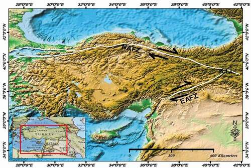
Anatolian plate (Figure 1) which is the subject of this study formed from the amalgamation of major lithospheric blocks during a long history of Tethyan subduction that dates back at least to the Cretaceous (Menant et al., 2016; Sengor. & Yilmaz., 1981; Van Hinsbergen et al., 2016). All previous geophysical and geological studies with recent tectonic maps of Anatolian plate besides the geographic information systems data confirmed the formation of the wide networks of fault systems in the study area. During Pliocene, the East Anatolian Fault Zone (EAFZ) as well as strike-slip fault systems formed. According to the strike of the segments, the EAFZ should comprise six segments (Saroglu et al., 1992). But Hempton et al. (1981) detected only five segments, while Barka and Kadinsky-Cade. (1988), based on fault geometry and seismic activity, they suggested that there could also be 14 different segments along the EAFZ. On the other side, the North Anatolian Fault Zone (NAFZ) structure is the most active seismically and disastrous with shallow focal depth earthquakes 10 km and a lower crustal depth of the crust (Türkelli et al., 2003). Western part of NAFZ section recognised with short recurrence of the ruptured fault segments. Additional information about extension at the depth of the NAFZ came from the lithospheric nature of the NAFZ proved by the discharged thermal fluids along the fault (Gülec et al., 2002; De Leeuw. et al., 2010). The NAFZ does not end at the Karliova triple junction, extends for (50 km) towards the south-east (Hubert Ferrari et al., 2009; Türkelli et al., 2003). The main NAFZ segments are the N110- 120_E eastern trending part, a northern convex central trending part, and a N75_E western trending part (Barka, 1992). There is a probability of increasing rapture failure pattern of NAFZ during the 20th century (Stein et al., 1997). According to Portner et al. (2018), today, Anatolian is in a complex tectonic regime described in three discrete neotectonic regions: The East Anatolian Contractional Province, the West Anatolian Extensional Province, and the Central of Anatolia Province (Şengör et al., 1985). Neotectonic evolution of Anatolian was formed by collision of the African and Arabian plates with the Eurasian plate along the Bitlis–Zagros suture zone to the east (Wilson & Bianchini, 1999). This evolution was controlled by the continuing northward motions of the African and Arabian plates regarding Eurasian plate. Anatolian westward extrusion along the North and East Anatolian fault zones was formed In the Middle-Late Miocene (Dewey & Sengor., 1979; Jackson & McKenzie., 1988; McKenzie, 1972; Sengor. & Yilmaz., 1981). There are original hypotheses for the Anatolians extrusion driving forces: (i) The rigid behaviour model of plate causes the Hellenic subduction retreat with subducting Arabian plate into Anatolian, which pushes and pulls Anatolian westward, respectively (Heidbach, 2005). (ii) A key role of this movement is the energy of gravitational potential (GPE) difference between a crust, which is thicker in eastern Anatolian and the crust, which is thinner to the west (Özeren & Holt, 2010). This means that the GPE gradient causes this westward movement of Anatolian plate. (iii) Ultimately, according to recent studies, the lithosphere drags above by the existence of a toroidal flow in the asthenosphere (Faccenna & Becker., 2010; Le Pichon & Kremer., 2010). The Anatolian was at one time a single plate that is presently being turned into many nanoplates proved by Assembling geophysical and GIS data. This paper proposed a practical method for linear faults detection that automatically extracts the linear anomalies from different gravity data sets within the study area. We have prepared linear fault dataset for abnormal seismic hazard zones within Anatolian by using Deep learning edge detection technique; we have tried to localise the distinct fault lines to find distinct tectonic nano plate boundaries.

Figure 1. Study area

2. Methodology

2.1. Geophysical data

This paper proved the formation of these nano tectonic plates and determined their boundaries by integrating and analysing massive remote sensing geophysical data sets:

2.2. Global geophysical datasets

• Global free air surface anomalies DTU10, (DTU10GRA_1 min) show the gravity variations over the global ocean as mapped by satellite (ERS-1 and ENVISAT). On land the field has been augmented with the best terrestrial gravity field complete global coverage. Gravity changes mainly caused by the changes in the attraction of mass under the surface. DTU10 ocean wide gravity field mapped with a resolution of 1 min by 1 min corresponding to 2 min by 2-minresolution at Equator (Andersen et al., 2010, 2010). The data downloaded from DTU Space at The Technical University of Denmark https://www.space.dtu.dk

• New global marine gravity model from CryoSat-2 and Jason-1 reveals buried tectonic structure. Combined new radar altimeter measurements from satellites CryoSat-2 and Jason-1 with existing data to construct a global marine gravity model that is two times more accurate than previous models. This was constructed to understand global tectonic processes and highlight the importance of satellite-derived gravity models as one of the primary tools for the investigation of remote ocean basins (Sandwell et al., 2014). It can be downloaded from EarthByte which is a universally leading eGeoscience collaboration between several Australian Universities, international centres of excellence and industry partners. https://www.earthbyte.org

• ETOPO1 global relief model (bedrock) ETOPO1 is a 1 arc-minute global relief model of Earth’s surface that integrates land topography and ocean bathymetry. Built from global and global data sets, developed by the National Geophysical Data Center (NGDC), an office of the National Oceanic and Atmospheric Administration (NOAA) (NOAA National Geophysical Data Center, 2009). Downloaded from https://www.ngdc.noaa.gov/mgg/global

2.3. Local geophysical dataset

• Local gravity data for Anatolian from Jason-1 satellite, which is a joint project between the NASA (United States) and CNES (France) space agencies provide a unique global view of the oceans and sea surface height anomalies that are impossible to gain using traditional ship-based sampling. It was launched in 7 December 2001 https://podaac.jpl.nasa.gov/JASON1 and began data collection on 15 January 2002 (Menard & Haines, 2001). The data downloaded from NASA Jet Propulsion Laboratory California Institute of Technology

2.4. GIS data and tables

• The 1:1 250,000 Scale Active Fault Map of Turkey from General Directorate of Mineral Research and Exploration, Special Publication Series-30 Ankara-Turkey (Emre et al., 2013). It can be downloaded from Mineral Research and Exploration General Directorate (MTA) which is a research organisation that provides data to improve mining sector and offers infrastructure services.

  1. https://www.mta.gov.tr

• Tectonic plate boundary data for the entire globe as a shape files data from United States Geological Survey (USGS), earthquakes pages (KMZ): downloaded from https://earthquake.usgs.gov

2.5. The techniques and softwares used in this study

• Convolutional Neural Network (CNN).

1. Tensor Flow, which is an end-to-end platform for building and deploying Machine Learning models (Abadi et al., 2015) downloaded from https://www.tensorflow.org

2. Keras libraries, Keras is a deep learning API written in Python, running on top of the machine learning platform TensorFlow for analysing gravity data to detect horizontal, vertical, northeast, northwest derivations (linear anomalies) to define distinct plates boundaries. (Chollet et al., 2015) Available at: https://github.com

SciPy, Fundamental library for scientific computing (Virtanen et al., 2020) downloaded from https://www.scipy.org

• Matplotlib library is a comprehensive library for creating static, animated, and interactive visualisations in Python. downloaded From https://matplotlib.org

• Image analysis and image enhancement techniques using remote sensing and geo-image processing software GEOMATICA 2020 downloaded from https://www.pcigeomatics.com

• ArcGis10.8 software from ESRI foundation for GIS overlay analysis. Downloaded From https://desktop.arcgis.com

2.6. Data preprocessing

Before linear features extraction process, this paper used enhancement toolbar of PCI GEOMATICA. This study applied quick adjustments to all image data used for linear features extraction, such as a Linear enhancement. Also adjusted the contrast and brightness, and also applied a more advanced contrast and brightness adjustment.

2.7. Fault network detecting

The Fault network is defined according to the following steps:

2.7.1. Linear anomalies detection by traditional edge detection

One of the important things in gravity data interpretation is linear anomaly because they show some important structural features. This analytic research faced serious challenges for active fault detection because of the complex structural setting inherited from previous Anatolian contractional tectonics. We have tried to localise the distinct fault lines in order to find distinct tectonic plate boundaries. The fundamental part of advanced image processing research is Line detection because of its prominent applications. When edges detected, then the information which is less relevant can be filtered out (Arbel´aez. et al., 2011, 2014; Bertasius et al., 2015). Traditional Edge detection techniques are categorised into two main types: 1. Gradient-Based and 2. Laplacian-Based. In the first type, the edges detected by finding the maximum and minimum in the first derivative of the image (Arbel´aez. et al., 2014; Chen. et al., 2014). while second type The Laplacian-based is used to find whether a pixel is on the dark or light side of an edge. The main types of gradient based: Horizontal edges, Vertical Edges and Diagonal Edges.

2.7.2. Linear anomalies detection by convolutional neural networks

Although there was a significant improvement in traditional edge detection methods by using low-level features (M. Leordeanu et al., 2014), but they are suffering from limitations. Neural networks can serve as nonlinear filters and fully trained to detect edges. Today, the most popular technique in the computer vision community is convolutional neural networks (CNNs) which have become more usable in many advanced tasks, from image classification (A. Krizhevsky et al., 2012; Simonyan & Zisserman, 2014), to semantic segmentation (L. C. Chen. et al., 2014; Long et al., 2015) and object detection (R. Girshick., 2015; R. Girshick. et al., 2014; Y. Li. et al., 2016; Ren. et al., 2015). There is a recent trend of using convolutional networks to perform linear features detection and learning high-level representations of natural images automatically because they have a strong capability to do the best job. Some well-known CNN-based methods have pushed forward this field considerably, such as Deep Edge (G. Bertasius et al., 2015), N4-Fields (Ganin. & Lempitsky, 2014), CSCNN Hwang. & Liu, 2015), Deep Contour (Shen. et al., 2015), and HED (Xie & Tu, 2017). This paper proposed the inception network, which was an important milestone in the development of CNN classifiers. This paper suggested a method consisting of many steps for fault Network detection using Remote Sensing Geophysical data (Gravity data). A practical method proposed for linear faults detection that automatically extracts the linear anomalies from different gravity data sets within the study area. The proposed inception model improved by the combination of multi directional and multi-scale filters. Then, the model trained by synthetic lineament patterns to detect a specific lineament patterns (horizontal, vertical and diagonal). This study has proposed wider model because deep networks suffer from over-fitting. The network originally would get a bit ‘wider’ rather than ‘deeper’ when having filters with multi sizes and multidirectional operate on the same level. This means our network will detect global and local geological features for all directions by using different sizes and directions of filters. Concatenating local features which extracted by small filters together with global features extracted by large filters will rich our map of nanoplates boarders.

2.7.3. Proposed inception neural network for nanoplates boundaries detection

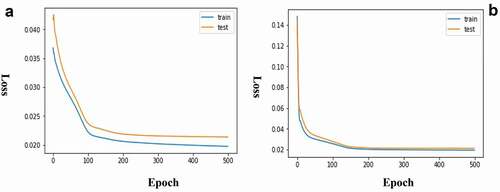
Our work deals with integrating global and local (Geophysical data sets) to improve the structural knowledge of the study area and to gain the potential of constraining quantitative details to hitherto unknown areas and reduces the ambiguity of geological interpretation. This paper also integrated the geological and geophysical data, both data represented as images and every image has multidirectional edges (vertical, horizontal and diagonal) which actually combining to form an image (Chen & Zhou, 2005; Lamontagne et al., 2003; Lunden et al., 2001; Yassaghi, 2006). Convolution operation was used with some filters for detecting these kinds of edges. To design deep learning convolutional neural network model, we have prepared big linear dataset for best known faults around the world, consisting from 2000 small images using augmentation technique. Then we have split the dataset into train and test folders. In order for fast computation of gradients this paper trained and tested this model by using the weights of filters in inception convolutional neural network (CNN) which was trained using gradient decent-based algorithms such as updated weights of efficient Adam’s version of stochastic gradient descent (SGD) with backpropagation algorithm with the Mean Absolute Error (MAE) loss function. To minimise the cost function for all training and validation data, the weights optimised model fitted and evaluated to avoid overfitting and underfitting by reviewing its performance over time. We have gotten a different diagnostic plot for each run and the train and validation traces plotted for each run at the end of each training epoch Figure 2. The model trained by calling the python fit () which is automatically split our training dataset into train and validation sets based on a percentage split specified via the validation_split argument. This function returns a variable called history that contains a trace of the loss. Then, the model error scores Root Mean Squared Error (RMSE) calculated. Finally, the final RMSE of the model on the test dataset calculated and printed its value 0.129. The model started with derivatives of the output layer and moved backwards towards the input layer. The weights of CNN kernels optimised by using tricks like regularisation, which is much efficient to chain the derivatives. Then, the model optimised by fine-tuned hyper-parameters. We implemented this model in TensorFlow open-source platform for Deep learning. It has a comprehensive, flexible ecosystem of tools, libraries and community resources.

Figure 2. Train and validation learning curves showing traces plotted for each run

A) Underfitting Model, B) fitting Model

2.7.4. Proposed network nature and architecture

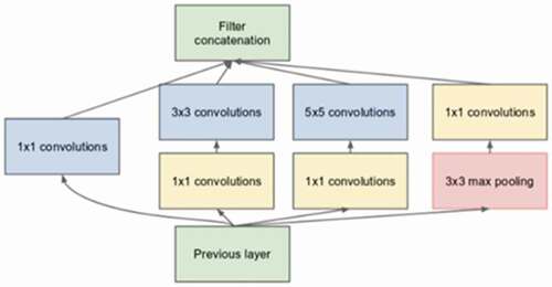
The key innovation of the inception model called the inception module. This is a block of parallel convolutional layers with different sized filters (e.g. 1 × 1, 3 × 3, 5 × 5) and 3 × 3 max pooling layer Figure 3, the results of which are then concatenated. (Szegedy et al., 2015);

Figure 3. Original inception module as described by (Szegedy et al., 2015)

We designed our network by modifying inception network and carefully designing a universal strategy to combine hierarchical CNN features. Our system performs very well in edge detection. The proposed inception method has two kinds of Feature extractor module: the first one comprises three modules of local feature extraction and the second one comprises three modules of global feature extraction. The major contributions of proposed inception network compared to the original inception networks are:

• The first module of local feature extraction consists of a block of parallel convolutional layers with two sized filters (1x1 with the number of filters equal to 24, 3 × 3 with a number of filters equal to 64 followed by 1 × 1 convolution, two 3 × 3 convolutions followed by 1 × 1 convolution and 3 × 3 max pooling layer followed by 1 × 1 convolution), the results of which are then added in Figure 4.

• The second module of local feature extraction consists of a block of parallel convolutional layers with two sized filters (1x1 with number of filters equal to 24 and factorised convolutions of filter size 5 × 5 to a combination of 1 × 5 and 5 × 1 convolutions with number of filters equal to 128 followed by 1 × 1 convolution, two factorised convolutions of filter size 5 × 5 followed by 1 × 1 convolution, and 3 × 3 max pooling layer followed by 1 × 1 convolution, the results of which are then added in Figure 5.

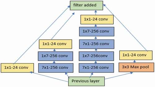
• The third module of local feature extraction comprises a block of parallel convolutional layers with two sized filters (1x1 with number of filters equal to 24, factorised convolutions of filter size 7 × 7 to a combination of 1 × 7 and 7 × 1 convolutions with number of filters equal to 256 followed by 1 × 1 convolution, two factorised convolutions of filter size 7x7 followed by 1 × 1 convolution, and 3 × 3 max pooling layer followed by 1 × 1 convolution, the results of which are then added in Figure 6.

• The proposed Inception model-maintained input channels without reducing by putting 1 × 1 convolution after 3x3,5x5,7x7 convolutions in order to gain informative features. Although this change is computationally expensive but this study used a very high-performance GPU machine to reduce the computation time.

• The architecture of the fourth, fifth and sixth global modules is the same as that of the first, second and third modules, with the difference of adding Dilation rate equals to two after 3 x 3, 5 × 5 and 7 × 7 convolutions in order to get global information, the benefit of this approach is that the receptive field of units in the network can grow exponentially with the number of layers/parameters as compared to non-dilated convolutions without loss of resolution or coverage. This approach helped to detect global fault system across the study area.

Figure 4. The architecture of first module of local feature extraction

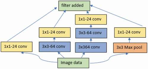
Figure 5. The architecture of second module of local feature extraction

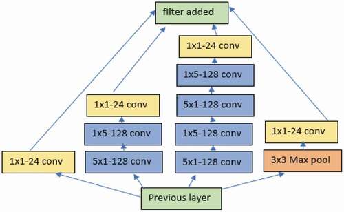
Figure 6. The architecture of third module of local feature extraction

2.7.4.1. Multiscale and multidirectional filters

The fundamental concept of any Inception Network is extracting features at varying scales and because of this enormous variation in the location of the geological information in our dataset, choosing the right kernel size for the convolution operation becomes tough. A larger kernel preferred for information that is distributed more globally (dilated 5 × 5 and dilated 7 × 7 filters), and a smaller kernel preferred for information that is distributed more locally (3x3,5x5 and 7 × 7 without dilation). Having filters with multiple sizes operate on the same level? The network essentially would get a bit ‘wider’ rather than ‘deeper’. In order to extract different direction (vertical, horizontal, diagonal and anti-diagonal) linear features through convolution, this study used filters whose weights automatically learned these directions during training this means training dataset contained these directions. All these extracted features then combined.

2.7.4.2. Proposed model parameters

Several Inception models proposed with a different number of layers and consequently a different number of parameters. For example, ResNet-50, ResNet-101, and ResNet-152 have around 26 M, 45 M, and 60 million parameters, respectively Recently, new networks have improved the ResNet model like Dense Net The number of parameters of Dense Net model is about half of those considered by ResNet. Better accuracy achieved with SENet SENet has 25 million parameters (Véstias, 2019). This study trained two different inceptions model the first one has about 13,203,197 total parameters because of the big filter numbers chosen for the modules like 768, 512 and 256 and the second one has about 6,109,485 total because of small filter numbers like 64, 128 and 256 the computation time for both models are (10 min.,45 s) and (4 min, 32 s).

2.7.4.3. Feature map Maths

Feature map values calculated according to the following formula (1), where the input image denoted by f and our kernel by h. The indexes of rows and columns of the result matrix marked with m and n, respectively.

(1) $G[m,n]=(f\ast h)[m,n]=\sum _j\sum _{k}h[j,k]f[m-j,n-k]$(1)

3. Results and discussion

3.1. Constructing nano plates boundaries and discussion

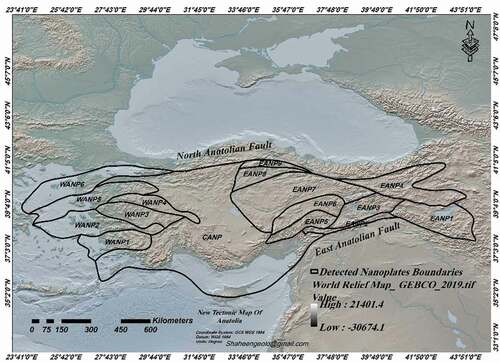
The construction of tectonic nano plates boundaries from extracted tectonic lineaments is a hard task. Choosing the subset of extracted faults for nanoplates boundaries done by depending on Anatolian, Turkey’s active and non-active fault layer with geological map of Turkey downloaded from Turkey (MTA: General Directorate of Mineral Research and Explorations organisation, Turkey). This work connected only adjacent detected fault lines of active tectonic Anatolian regions which were formed by complex tectonic process. The second step, the lineaments spatially correlated against the gravity anomalies which represent gravity signatures that reflect best tectonic boundaries; we have integrated different geophysical data from different sources and converted these outputs to GIS means to construct the final boundaries map successfully after excluding the lines that are far from active seismic areas. Then, we have overlaid all these outputs using GIS software ArcGIS10.8. In order to define these nano plates, we have divided the study area to three zones: East Anatolian, West Anatolian and Central Anatolian. For best accuracy in identifying these faults networks this paper considered the results of analyzes for all data, started by previewing the maps of the multidirectional Cardiant Linear anomalies results (Horizontal, Vertical, Northeast and Northwest,) of (New global marine gravity model got from CryoSat-2 and Jason-1 satellites reveals 2014) Figure (7) with (Global gravity free air surfaces anomalies DTU10, (DTU10GRA_1 min) gradients for Anatolian Figure 8. Best linear anomalies resulted from these Gravity data were the Horizontal gradient linear anomaly of (DTU10GRA_1 min) for study area and matched with MTA fault lines approximately 80% Figure (8) and also, we have founded new fault lines in different directions helped us for best connecting old fault lines with new ones to model boundaries map. We have extracted fault lines from these linear anomalies by explained Deep learning edge detection method, which converted to fault lines by OpenCV Libraries in Anaconda platform and all these layers overlaid on high resolution global relief model of (1) min ETOPO1 (bedrock) as background map Figures 9,10. The final constructed map of nanoplates boundaries for all Anatolian Figure 11.

Figure 7. Multidirectional cardiant linear anomalies of new global marine gravity model obtained from CryoSat-2 and Jason-1 satellites reveals 2014

A) Horizontal, B) Vertical, C) Northeast, D) Northwest

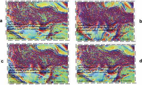
Figure 8. Multidirectional cardiant linear anomalies of global free air surfaces anomalies DTU10, (DTU10GRA_1 min)

A) Horizontal, B) Vertical, C) Northeast, D) Northwest

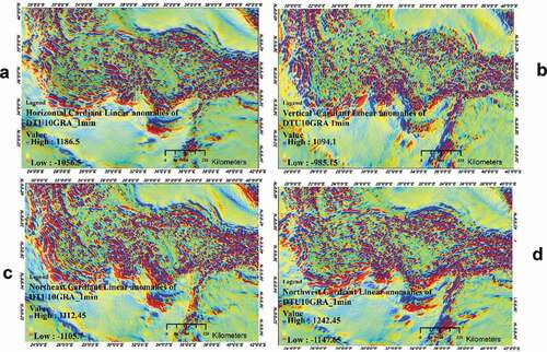
Figure 9. Extracted fault lines from multidirectional cardiant linear anomalies of global free air surfaces anomalies DTU10, (DTU10GRA_1 min)

A) Horizontal, B) Vertical, C) Northeast, D) Northwest. A) Horizontal, B) Vertical, C) Northeast, D) Northwest

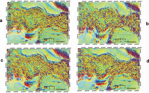
Figure 10. Extracted fault lines from multidirectional cardiant linear anomalies of new global marine gravity model obtained from CryoSat-2 and Jason-1 satellites reveals 2014

A) Horizontal, B) Vertical, C) Northeast, D) Northwest.

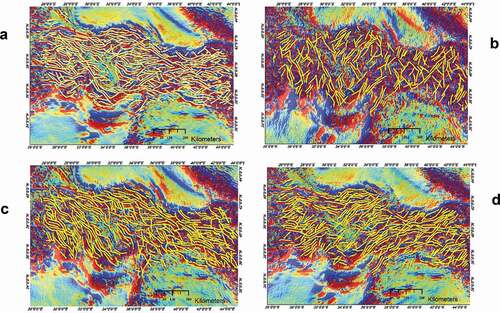
Figure 11. Constructed nanoplates boundaries

3.1.1. Geological knowledge agreement with extracted features

Besides MTA map, this paper is based on the determination of the deep fault network of nano plate boundaries on main and branching fault segments along the NAFZ and ENFZ. Segments and sub segments boundaries are defined according to the following tectonic studies and models of Anatolian.

• Bulut et al. (2012) identified the segmentation and kinematics along the full East Anatolian Fault Zone (EAFZ) using well-located earthquakes reported by a dense global seismic network. They found internal deformation of the fault system and surrounding splay faults. They found the followings:

  1. The EAFZ indicated by NE-SW and E-W oriented sub-segments that are sub-parallel to the overall trend of the fault zone.

  2. They documented progressive interaction between the major branch of the EAFZ and its secondary structures.

  3. The EAFZ also characterised by several smaller _N-S and E-W- oriented subsegments.

The main EAFZ segments:

1. The Gölbasi – Celikhan – Pütürge area

2. The Pütürge-Sivrice-Elazig segments in the central part of the EAFZ characterised by several basins producing strike-slip faulting, these segments currently host the highest seismicity rate throughout the EAFZ.

3. The Karliova-Bingöl segment of the EAFZ, most seismic events in this area had a dominant thrust-type fault mechanism.

• Seyitoğlu, et al., (2018) re-evaluated the marginal strike-slip faults of the segmentations of 41 marginal strike-slip faults on the hinterland of the Bitlis–Zagros suture zone which determined using high-resolution satellite images(Seyitoglu, et al., 2019) .

• Gasperini et al. (2021) observed in the North Anatolian fault system, three brands of deformation: almost perfect strike-slip faults, aligned mainly E–W; NE/SW-aligned axes of transpressive structures; NW/SE- aligned trans-tensional depressions. Fault segmentation develops at different scales, but major segments occur along three major right-lateral oversteps, which delaminate main fault branches, from east to west: (i) the transtensive Cinarcik segment; (ii) the Central (East and West) segments; and (iii) the westernmost Tekirdag segment.

• McNeill et al. (2004) used Side‐scan sonar data within the North Aegean Trough which is tectonically restrained by the projection of the North Anatolian Fault from western Turkey and the Sea of Marmara into the Aegean and they determined the existence of strike‐slip deformation associated with the westward continuation of the North Anatolian Fault. They defined two kinds of faulting: (1) transtensional basin‐bounding faults controlling the significant vertical topography of the basin and (2) dextral faulting within the central basin. These styles of faulting merge at greater depths into a single fault.

3.2. Matching between linear features of GIS and extracted linear features

Matching GIS objects with features extracted from any image called feature matching in the relevant literature and in this paper, too. Linear feature matching deals with straight lines, polygons, groups of straight lines, and curves. We assume the satellite image and the GIS data have been approximately matched interactively by 3 or 4 corresponding points. So, there is a geometric reference, which is established by a common coordinate system. Then, our goal is to find image features that match best with the objects in the GIS. The strategy is to avoid complex search problems by using the most significant lines extracted from the satellite image. The optimum global solution of a matching problem given by a mapping that minimises a weighted sum of several measures where small values of measures represent good correspondences. We are not using this approach here, since we consider solving the problem by local strategies the procedure is a comparison of GIS objects and image.

Features where hypotheses for image features corresponding to the GIS objects generated within a defined searching space. The strategy is to establish the matches that show highest probability. Conflicting matches are evaluated using the following tools and measures:

1. Buffer tool

Buffers are usually used to delineate protected zones around features or to show areas of influence. This paper used the multi-ring buffer tool of ARCGIS 8.0 to classify the areas around every important fault line feature in MTA vector GIS data into near, moderate distance, and long-distance classes than chose those nearest extracted linear features to the important fault line after overlying the two kinds vector data.

1. Length

Hence, our strategy is to find correspondences for the longest features first and to proceed successively with the shorter ones.

1. Parallelism:

When matching straight lines, parallelism is the major criterion. It offers reliable correspondences for the direction that is orthogonal regarding the lines. Parallelism measured by the direction of two lines or by the change of their distances.

3.3. The tectonic evolution of nano plates

3.3.1. Tectonic evolution of East Anatolian nanoplates

After analysing, the results this paper detected (9) nano plates in the East Anatolian. we suggest the tectonic evolution of these nano plates begun after forming of the East Anatolian Fault System between Late Miocene‐Early Pliocene (Hempton et al., 1981; Şengör et al., 1985), when the Arabian and Eurasian plates collided upon the closure of the southern branch of the Neo-Tethys ocean (Nouri et al., 2016; Okay et al., 2010; Sengor. & Yilmaz., 1981). The earliest deformation stage in the southeastern Anatolian occurred from the Palaeocene to middle Eocene times, which corresponds to NE-SW extension in the upper plate, which caused slab rollback (Kaymakci et al., 2010). Because of this expansion group of faults formed and many of the old faults extended vertically and horizontally because of this expansion four nano plates formed: East Anatolian Nano plate1, ENNP2, ENNP3 and ENNP4 Figure 11. The more recent plate movements directed mainly westward and associated with strike-slip faults extension tectonics which led to formation of the EANP 5, EANP 6, EANP7. The NAFZ splays into branches east of the Marmara region, forming a westward widening deformation zone under the influence of the N/S extensional Aegean regime (Dewey & Sengor., 1979; McKenzie, 1972; Le Pichon et al., 2015; Şengör et al., 1985) this led to formation of EANP8, EANP9.

3.3.2. Tectonic evolution of West Anatolian nanoplates

Recent tectonic regime of west Anatolia formed by subduction along the Aegean Trench. Since at least 35–30 million years the Aegean Trench migrates to the southward, contributing to extension in the overriding plate and thinning of the Aegean continental lithosphere. A westward pulling force on the Anatolian plate caused by subduction processes at the Hellenic arc which also causes extension in the western portion of the Anatolian plate, leading to complexity to fault geometry and hence rupture propagation in western sections of the NAFZ (Flerit et al., 2004; Pondard et al., 2007). This led to the formation of the following Nano plates: WANP1, WANP2, WANP3, WANP4, WANP5, and WANP6.

3.3.3. Tectonic evolution of Central Anatolian nanoplate

Central Anatolian dominated by trans-tension, as expressed by increased exhumation rates and extensional basin formation related to the Central Anatolian fault zone (Kocyiǧit and Beyhan, 1998; Fayon & Whitney, 2007). Since Miocene Central Anatolian plateau and the Eastern Anatolian plateau formed a single plateau. Deformation within Central Anatolian facilitated the voluminous volcanism of the Central Anatolian (Toprak & Göncüolu, 1993). This study detected a single nano plate in the Central Anatolian Plate and named it (CANP).

4. Conclusion

The Anatolian was at one time a single plate that is currently separated into many nano plates. We concluded through our current study that the best geological explanation for the increasing of Anatolian seismic activity related to the behaviour of these Nano plates. This paper made the following conclusions:

• This study for the first-time confirmed that the Anatolian plate broken into a group of small nanoplates in the three regions within Anatolian and detected formation of (9) nano plates in the East Anatolian region with (6) nanoplates in the West Anatolian region and single nanoplate in the central Anatolian region.

• For the first time, we have developed Inception CNN Model for geological fault network detection.

• Anatolian behaviour changed after forming of these Nano plates because we have dealing with group of small size plates and not a single plate. Every Nano plate affects the adjacent plates with different forces therefore we advise for more studies about behaviour of these Nano Plates using advanced techniques supported by directions of movement. These kinds of studies will explain the increased seismic activity along Anatolian and also, we recommend for developing new Seismic Hazard map for Anatolian considering this study’s results.

Disclosure statement

No potential conflict of interest was reported by the author(s).

References

- Abadi, M., Agarwal, A., Barham, P., Brevdo, E., Chen, Z., Craig Citro, G. S., Corrado, A. D., Dean, J., Devin, M., Ghemawat, S., Goodfellow, I., Harp, A., Irving, G., Isard, M., Jozefowicz, R., Jia, Y., Kaiser, L., Kudlur, M., Levenberg, J., Mané, D., … Zheng, X. TensorFlow: Large-scale machine learning on heterogeneous systems, 2015. Google Brain Team. Software available from tensorflow.org.
- Andersen, O. B., Knudsen, P., & Berry, P. (2010). The DNSC08GRA global marine gravity field from double retracked satellite altimetry. Journal of Geodesy, 84 (3), 191–199. [17sep 2019] Accessed. https://doi.org/https://doi.org/10.1007/s00190-009-0355-9
- Arbel´aez., P., Maire., M., Fowlkes., C., & Malik., J. Contour detection and hierarchical image segmentation. (2011). IEEE Transactions on Pattern Analysis and Machine Intelligence, 33(5), 898–916. 1, 2, 4, 5, 6, 7, 8. https://doi.org/https://doi.org/10.1109/TPAMI.2010.161
- Arbel´aez., P., Pont-Tuset., J., Barron, J. T., Marques., F., & Malik, J., 2014. Multiscale combinatorial grouping. In IEEE CVPR, Columbus, OH, USA. IEE Computer Society. 328–335.
- Barka, A. (1992). The North Anatolian Fault zone. Ann. Tecton, issue6, 164_195.
- Barka, A. A., & Kadinsky-Cade., K. Strike-slip fault geometry in Turkey and its fluence on earthquake activity. (1988). Tectonics, 7(3), 663–684. 7/3. https://doi.org/https://doi.org/10.1029/TC007i003p00663
- Bertasius, G., Shi, J., & Torresani., L., 2015 Deep Edge: A multiscale bifurcated deep network for top-down contour detection. In IEEE CVPR,Boston, MA, USA IEE Computer Society. 4380–4389.
- Bulut, F., Bohnhoff, M., Eken, T., Janssen, C., Kılıç, T., & Dresen, G. (2012). The East Anatolian Fault Zone: Seismotectonic setting and spatiotemporal characteristics of seismicity based on precise earthquake locations. Journal of Geophysical Research: Solid Earth, 117(B7). n/a–n/a. 1759- 1768 https://doi.org/https://doi.org/10.1029/2011jb008966.
- Chen., L. C., Papandreou., G., Kokkinos., I., Murphy., K., & Yuille, A. L., 2014 Semantic image segmentation with deep convolutional nets and fully connected crfs. Cornel University. arXiv preprintarXiv:1412.7062.
- Chen, S., & Zhou, Y. (2005). Classifying depth-layered geological structures on Landsat TM images by gravity data: A case study of the western slope of Songliao Basin, northeast China. Int. J. Remote Sens, Volume 26, Issue 13262741–262754.
- Chollet, F. & others, 2015. Keras. Github. Available at: https://github.com/fchollet/keras.
- De Leeuw., G. A. M., Hilton., D. R., Güleç., N., & Mutlu, H. (2010). Global and temporal variations in CO2/3He, 3He/4He and δ13C along the North Anatolian fault zone, Turkey. Applied Geochemistry, 25(4), 524–539. https://doi.org/https://doi.org/10.1016/j.apgeochem.2010.01.010
- Dewey, J. F., & Sengor., A. M. C. (1979). Aegean and surrounding regions: Complex multi-plate and continuum tectonics in a convergent zone. Geological Society of America Bulletin, 90(1), 84–92. https://doi.org/https://doi.org/10.1130/0016-7606(1979)90<84:AASRCM>2.0.CO;2
- Emre, Ö., Duman, T. Y., Özalp, S., Elmacı, H., Olgun, Ş., & Şaroğlu, F., 2013. Active fault map of Turkey with and explanatory text. General directorate of mineral research and exploration, special publication series-30. [19 Sep, 2019]. General directorate of mineral research and exploration turkey. https://www.mta.gov.tr/eng/maps/active-fault-1250000.
- Faccenna, C., & Becker., T. W. (2010). Shaping mobile belts by small-scale convection. Nature, 465(7298), 602–605. https://doi.org/https://doi.org/10.1038/nature09064
- Fayon, A. K., & Whitney, D. L. (2007). Tectonic vs. magmatic processes and the resetting of apatite fission track ages: An example from the Nide Massif, Turkey. Tectonophysics, 434(1–4), 1–13. https://doi.org/https://doi.org/10.1016/j.tecto.2007.01.003
- Flerit, F., Armijo., R., King, G., & Meye, B. (2004). The mechanical interaction between the propagating North Anatolian fault and the back‐arc extension in the Aegean, earth planet. Sci. Lett, 224(3–4), 347–362. https://doi.org/https://doi.org/10.1016/j.epsl.2004.05.028
- Ganin., Y., & Lempitsky, V., 2014 N4-Fields: Neural network nearest neighbor fields for image transforms. In ACCV, Cornell University. 536–551.
- Gasperini, L., Stucchi, M., Cedro, V., Meghraoui, M., Ucarkus, G., & Polonia, A. (2021). Active fault segments along the North Anatolian Fault system in the Sea of Marmara: Implication for seismic hazard. . Mediterranean Geoscience Reviews, 3(1), 29–44. https://doi.org/https://doi.org/10.1007/s42990-021-00048-7
- Girshick., R., 2015 Fast R-CNN. In IEEE ICCV,Santiago, Chile.International Conference on Computer Vision (ICCV). 1440–1448.
- Girshick., R., Donahue., J., Darrell., T., & Malik, J., 2014. Rich feature hierarchies for accurate object detection and semantic2014 Cornell University.
- Gülec, N., Hilton, D. R., & Mutlu, H. (2002). Helium isotope variations in Turkey: Relationship to tectonics, volcanism and recent seismic activities. Chemical Geology, 187(1–2), 129–142. https://doi.org/https://doi.org/10.1016/S0009-2541(02)00015-3
- Heidbach, O. (2005). Velocity field of the Aegean-Anatolian region from 3D finite element models. F. Wenzel, 169–185. Springer.
- Hempton, M. R., Dewey., J. F., & Saroglu, F. (1981). The East Anatolian transform fault: Along strike variations in geometry and behavior. EOS Trans, Issue 62, 393.
- Hubert Ferrari, A., King, G., van der Woerd, J., Villa, I., Altunel, E., & Armijo, R. (2009). Long-term evolution of the North Anatolian fault: New constraints from its eastern termination. In Geological Society, London, Special Publications. Van j., Hinsbergen & D. Hunter Eds., 2007, Matplotlib: A 2D graphics environment, computing in science & engineering, 9, no. 3, pp. 90–95, 2007 Vol. .
- Hwang., J. J., & Liu, T. L., 2015. Pixel-wise deep learning for contour detection. Cornell University. arXiv preprint arXiv:1504.01989, 2015.
- Jackson, J., & McKenzie., D. P. (1988). The relationship between plate motion and seismic moment tensors, and the rates of active deformation in the Mediterranean and Middle-East. Geophysical Journal International, 93(1), 45–73. https://doi.org/https://doi.org/10.1111/j.1365-246X.1988.tb01387.x
- Kaymakci, N., Inceöz, M., Ertepinar, P., & Koc¸, A. (2010). Late cretaceous to recent kinematics of SE Anatolian (Turkey). In M. Sosson, N. Kaymakci, R. Stephenson, V. Starostenko, A. Koçyiǧit, & A. Beyhan Eds., 1998. A new intracontinental transcurrent structure: The Central Anatolian Fault Zone. Tectonophysics, 284 (3-4 . Vol. 317–336
- Koçyiǧit A., and Beyhan, A., (1998). A new intracontinental transcurrent structure: The Central Anatolian Fault Zone, Turkey. Tectonophysics, 284 (3–4), 317–336
- Krizhevsky, A., Sutskever., I., & Hinton, G. E. (2012). Imagenet classification with deep convolutional neural networks. American for Comuting Machinary. ACM digital library. In NIPS (pp. 1097–1105).
- Lamontagne, M., Keating, P., & Perreault, S. (2003). Seismo-tectonic characteristics of the lower St. Lawrence seismic zone, Quebec: Insights from geology, magnetics, gravity and seismic. Canadian J Earth Sci, pages: 317–336. Issue 2 Volume 40.
- Le Pichon, X., & Kremer., C. (2010). The Miocene-to-present kinematic evolution of the Eastern Mediterranean and Middle East and its implications for dynamics. Annual Review of Earth and Planetary Sciences, 38(1), 323–351. https://doi.org/https://doi.org/10.1146/annurev-earth-040809-152419
- Le Pichon, X., Şengeor, A. M. C., Kende, J., I˙mren, C., Henry, P., Grall, C., & Karabulut, H. (2015). Propagation of a strike slip plate boundary within an extensional environment: The westward propagation of the North Anatolian Fault. Canadian Journal of Earth Sciences Volume 53 .number11. https://doi.org/https://doi.org/10.1139/cjes-2015-0129
- Leordeanu, M., Sukthankar., R., & Sminchisescu, C. (2014). Generalized boundaries from multiple image interpretations. IEEE Transactions on Pattern Analysis and Machine Intelligence, 36(7), 1312–1324. https://doi.org/https://doi.org/10.1109/TPAMI.2014.17
- Li., Y., He., K., & Sun, J., 2016 R-fcn: Object detection via region based fully convolutional networks. In NIPS, 379–387.NIPS'16: Proceedings of the 30th International Conference on Neural Information Processing Systems. American computing machinery. ACM digital Library.
- Long, J., Shelhamer., E., & Darrell, T., 2015. Fully convolutional networks for semantic segmentation. In IEEE Conference on Computer Vision and Pattern Recognition (CVPR), 2015, Boston, MA, USA. pp. 3431-3440, doi: https://doi.org/10.1109/CVPR.2015.7298965.I
- Lunden, B., Wang, G., & Wester, K. (2001). A GIS based analysisof data from Landsat TM, airborne geophysical measure-ments, and digital maps for geological remote sensing in the Stockholm region, Sweden. Int. J. Remote Sens, 22517–22532. Volume 22. Issue4. https://doi.org/https://doi.org/10.1080/01431160050505838
- McKenzie, D. P. (1972). Active tectonics of the Mediterranean region. Geophysical Journal International, 30(2), 109–185. https://doi.org/https://doi.org/10.1111/j.1365-246X.1972.tb02351.x
- McNeill, L. C., Mille, A., Minshull, T. A., Bull, J. M., Kenyon, N. H., & Ivanov, M. (2004). c Fault into the North Aegean Trough: Evidence for transtension, strain partitioning, and analogues for Sea of Marmara basin models. Tectonics, 23(2). Volume 23. issue 2. pages23-36 https://doi.org/https://doi.org/10.1029/2002tc001490.
- Menant, A., Jolivet, L., & Vrielynck, B. (2016). Kinematic reconstructions and magmatic evolution illuminating crustal and mantle dynamics of the eastern Mediterranean region since the late Cretaceous. Tectonophysics, 675, Issue1. 103–140. https://doi.org/https://doi.org/10.1016/j.tecto.2016.03.007.
- Menard, Y., & Haines, B., 2001. “Jason-1 CALVAL Plan”, JPL Ref: TP2-J0-PL-974-CN (PO. DAAC). Accessed [18 Jan 2020]. ERTHDATA.
- NOAA National Geophysical Data Center. 2009: ETOPO1 1 Arc-minute global relief model. NOAA National Centers for Environmental Information. Accessed [20 AUG, 2019].
- Nouri, F., Azizi, H., Golonka, J., Asahara, Y., Orihashi, Y., Yamamoto, K., Tsuboi, M., & Anma, R. (2016). Age and petrogenesis of Na-rich felsic rocks in western Iran: Evidence for closure of the southern branch of the Neo-Tethys in the late Cretaceous: Tectonophysics.Issue 3 671, 151–172. https://doi.org/https://doi.org/10.1016/j.tecto.2015.12.014
- Okay, A. I., Zattin, M., & Cavazza, W. Apatite fission-track data for the Miocene Arabia-Eurasia collision. (2010). Geology, 38(1), 35–38. https://doi.org/https://doi.org/10.1130/G30234.1
- Özeren, M. S., & Holt, W. E. The dynamics of the eastern Mediterranean and eastern Turkey. (2010). Geophysical Journal International, 183(3), 1165–1184. https://doi.org/10.1111/j.1365-246X.2010.04819.x
- Pondard, N., Armijo., R., King, G. C. P., Meyer., B., & Flerit, F. Fault interactions in the Sea of Marmara pull‐apart (North Anatolian Fault): Earthquake clustering and propagating earthquake sequences. (2007). Geophysical Journal International, 171(3), 1185–1197. https://doi.org/https://doi.org/10.1111/j.1365-246X.2007.03580.x
- Portner, D. E., Delph, J. R., Biryol, C. B., Beck, S. L., Zandt, G., Özacar, A. A., Sandvol, E., & Türkelli, N. (2018). Subduction termination through progressive slab deformation across Eastern Mediterranean subduction zones from updated P-wave tomography beneath Anatolian. Geosphere. 14(3), 907–925. https://doi.org/https://doi.org/10.1130/GES01617.1
- Ren., S., He., K., Girshick., R., & Sun., J., 2015 Faster R-CNN: Towards real-time object detection with region proposal networks. In NIPS '15: Proceedings of the 28th International Conference on Neural Information Processing Systems - Volume 1, cambridge MA USA. ACM digital library.91–99.
- Sandwell, D. T., Muller, R. D., Smith, W. H. F., Garcia, E., & Francis, R. (2014). Science. New Global Marine Gravity Model from CryoSat-2 and Jason-1 Reveals Buried Tectonic Structure, 346 (6205), 6567. [11 Jan 2020] Accessed. https://doi.org/https://doi.org/10.1126/science.1258213
- Saroglu, F., Emre., O., & Kuscu, I. (1992). The East Anatolian fault zone of Turkey. Ann. Tectonic, VI, Issue 3.99–125.
- Şengör, A. M. C., Görür., N., & Şaroğlu, F. (1985). Strike‐slip faulting and related basin formation in zones of tectonic escape: Turkey as a case study. In Strike‐Slip Deformation, Basin Formation, and SedimentationEds., K. T. Biddle & N. Christie‐Blick Soc. econ. paleontol. mineral Spec. Publ. Vol. 37 227–264
- Sengor., A. M. C., & Yilmaz., Y. (1981). Tethyan evolution of Turkey. A plate tectonic approach. Tectonophysics, 75(3–4), 181–241. https://doi.org/https://doi.org/10.1016/0040-1951(81)90275-4
- Seyitoğlu, G., Esat, K., Kaypak, B., Toori, M., & Aktuğ, B. (2018). Internal Deformation of Turkish–Iranian Plateau in the Hinterland of Bitlis–Zagros Suture Zone. Tectonic and Structural Framework of the Zagros Fold-Thrust Belt, 161–244. https://doi.org/https://doi.org/10.1016/b978-0-12-815048-1.00010
- Seyitoğlu, G., Esat, K., Kaypak, B., Toori, M., & Aktuğ, B. (2018). Internal deformation of Turkish–Iranian Plateau in the Hinterland of Bitlis–Zagros Suture Zone. Tectonic and Structural Framework of the Zagros Fold-Thrust Belt, Volume 3.Issue2.161–244. https://doi.org/https://doi.org/10.1016/b978-0-12-815048-1.00010-x
- Shen., W., Wang., X., Wang., Y., Bai., X., & Zhang., Z., 2015 Deep- Contour: A deep convolutional feature learned by positive sharing loss for contour detection. In Proceedings of the IEEE Conference on Computer Vision and Pattern Recognition (CVPR)IEEE CVPR,SEMANTIC SCHOLAR. Boston, MA, USA.3982–3991.DOI:https://doi.org/10.1109/CVPR.2015.7299024
- Simonyan, K., & Zisserman, A., 2014. Very deep convolutional networks for large-scale image recognition. Cornell University.arXiv preprint arXiv:1409.1556.
- Stein, R. S., Barka., A. A., & Dieterich, J. H. Progressive failure on the North Anatolian Fault since 1939 by earthquake stress triggering. (1997). Geophysical Journal International, 128(3), 594–604. https://doi.org/https://doi.org/10.1111/j.1365-246X.1997.tb05321.x
- Szegedy, C., Liu., W., Jia, Y., Sermanet., P., Reed., S., Anguelov., D., Erhan, D., Vanhoucke., V., & Rabinovich, A., 2015. Going deeper with convolutions. In IEEE CVPR, Boston, MA, USA (602), 2015 IEEE Conference on Computer Vision and Pattern Recognition (CVPR), pp. 1-9, doi: https://doi.org/10.1109/CVPR.2015.7298594.
- Toprak, V., & Göncüolu, M. C. (1993). Tectonic controls on the evolution of the Neogene-Quaternary central anatolian volcanic province. Geological Journal, 28(3–4), 357–369. https://doi.org/https://doi.org/10.1002/gj.3350280314
- Türkelli, N., Sandvol, E., Zor, E., Geok, R., Bekler, T., Al-Lazki, A., Karabulut, H., Kuleli, S., Eken, T., Gurbuz, C., Bayraktutan, S., Seber, D., & Barazangi, M. Seismogenic zones in eastern Turkey. (2003). . Geophysical Research Letters, 30(24), 8039. https://doi.org/https://doi.org/10.1029/2003GL018023
- Van Hinsbergen, D. J. J., Maffione, M., Plunder, A., Kaymakcı, N., Ganerød, M., Hendriks, B. W., Corfu, F., Gürer, D., de Gelder, G. I. N. O., Peters, K., McPhee, P. J., Brouwer, F. M., Advokaat, E. L., & Vissers, R. L. M. (2016). Tectonic evolution and paleogeography of the Kırşehir block and the central anatolian ophiolites, Turkey. Tectonics, 35(4), 983–1014. https://doi.org/https://doi.org/10.1002/2015TC004018
- Véstias, M. P. (2019). A Survey of convolutional neural networks on edge with reconfigurable computing. Algorithms, 12(8), 154. https://doi.org/https://doi.org/10.3390/a12080154
- Virtanen, P., Gommers, R., Oliphant, T. E., Haberland, M., Reddy, T., Cournapeau, D., Burovski, E., Peterson, P., Weckesser, W., Bright, J., van der Walt, S. J., Brett, M., Wilson, J., Millman, K. J., Mayorov, N., Nelson, A. R. J., Jones, E., Kern, R., Larson, E., Carey, C. J., & van Mulbregt, P. (2020). SciPy 1.0: Fundamental algorithms for scientific computing in python. Nature Methods, 17(3), 261–272. https://doi.org/https://doi.org/10.1038/s41592-019-0686-2
- Wilson, M., & Bianchini, G. (1999). Tertiary–Quaternary magmatism within the Mediterranean and surrounding regions. In B. Durand, L. Jolivet, F. Horvath, & M. Seranne (Eds.), The Mediterranean Basins: Tertiary extension within the alpine orogen. geological society (Vol. 156, pp. 141–168). Special Publications.
- Xie, S., & Tu, Z. Holistically-nested edge detection 2017. In International Journal of Computer Vision Volume 125 Issue 1-3 pp 3–18 .
- Yassaghi, A. (2006). Integration of Landsat imagery interpreta-tion and geomagnetic data on verification of deep-seated transverse fault lineaments in SE Zagros, Iran. Int. J. Remote Sens, Volume 27, Issue 20. 274529–274544.