Epistemic uncertainty in the kinematics of global mean sea-level rise since 1993 and its dire consequences

ABSTRACT

Recent studies reported an ambiguous global sea level acceleration during the satellite altimetry (SA) era (1993–2017). New SA data created an opportunity to resolve this issue. In this study, two competing kinematic models to represent global mean sea level anomalies are compared. The first model consists of an initial velocity and uniform acceleration. The second model replaces the initial velocity and acceleration with a trend and a representation of a long periodic lunar subharmonic of period 55.8 y, which is determined to be statistically significant at globally distributed tide gauge records. The models also include parameters for the periodic effects of lunisolar origin with periods 18.6 y and 11.1 y annual, and biannual variations in 10-day average of globally SA measurements during 1993–2022. Generalized least squares solutions yielded updated statistically significant estimates for all the model parameters and their statistics for both models. However, the outcome failed to resolve the ambiguity of uniform acceleration in global mean sea level confounded with the long periodic lunar subharmonic of period 55.8 y during this period. This epistemic uncertainty will have a dire impact on climate change risk assessments as demonstrated through the prospective comparison of both kinematic models.

KEYWORDS:

• Satellite altimetry
• tide gauge
• GMSL acceleration
• lunar subharmonics
• climate change

… the real purpose of the scientific method is to make sure nature hasn’t misled you into thinkingyou know something you actually don’t know.

R.M. Pirsig, The Art of Motorcycle Maintenance.

1. Introduction

Evidence for the global mean sea level (GMSL) rising faster during the 20^th and 21^st centuries with global warming is an important indicator in assessing anthropogenic contributions to the climate change mechanisms.

In the past, several studies investigated the presence of global acceleration during the 20^th century in sea-level rise using Satellite Altimetry (SA) data. For instance, Yi et al. (2015) reported an increase in GMSL, which can be translated into an average acceleration of 0.28 mm/y since 2010. Davis and Vinogradova (2017) reported an acceleration along the east coast of North America up to 0.30 mm/y², Dieng et al. (2017) determined an increase of about 0.8 mm/y in the GMSL velocity since 2004, equivalent to an average acceleration of 0.062 mm/y². More recently, Nerem et al. (2018) reported 0.084 ± 0.025 mm/y² GMSL acceleration since 1993 inferred from the globally averaged SA time series. Soon after, Ablain et al. (2019) reported another estimate of GMSL acceleration, 0.12 ± 0.07 mm/y².

In contrast to SA, tide gauge (TG) measurements sample only local and regional sea level variations. Their limited global distribution is prohibitive in making a conclusive inference about the GMSL trend and a uniform acceleration. However, TG can serve effectively as a consilience tool to verify SA findings about the GMSL rise because of their long records. A plethora of investigations during the last two decades indicated global sea level accelerations and decelerations. Some of them include Woodworth (1990), deceleration and acceleration; Douglas (1992) deceleration; Holgate and Woodworth (2004), acceleration; Church and White (2006), acceleration followed by deceleration; Jevrejeva et al. (2006), acceleration; International Panel on Climate Change, (2007), acceleration; Woodworth et al. (2009) acceleration followed by deceleration; Houston and Dean (2011), no acceleration; Watson (2011), a regional deceleration.

These spatio-temporal alternating accelerations and decelerations at TG stations were recognised as early as 1990s (Parker, 1992) and are explained effectively by transient/episodic changes due to the inverted barometer, wind, sea surface temperature etc. effects, as well as long periodic oscillations of the sea level of astronomical origin at multi-decadal frequencies excited by compounding mechanisms of various natural forcings.

In the past, two different exciting mechanisms for compounding in relation to climate change were suggested. Munk et al. (2002) conjured harmonic beating with the necessary conditions for generating subharmonics of the periods $P_A\mathrm{a}\mathrm{n}\mathrm{d}{P}_B$. The other mechanism proposed by Keeling and Whorf (1997) involves repeat coincidences and necessary conditions due to the events of near-perfect constructive interference that occurs at given intervals.

Under both scenarios, ocean and/or meteorological forcings materialise as natural broad band sea level variations and modulate orbital forcing, such as lunar nodal tide, thus their interplay leading to multi-decadal scale sea level variations in relation to the regression of the lunar node, which completes its cycle in P = 18.613 y, to produce sub- and super subharmonics as multiples of lunar node period.

The compounding of periodic sea level variations and their materialisations in sea level variations at multi-decadal scales is not speculative. For instance, Yndestad et al. (2008) reported that the water-property time-series show mean variability correlated to a subharmonic cycle of the nodal tide of about 74 y. They also have found significant correlations between dominant Atlantic water temperature cycles and the 18.6-y lunar nodal tide, and for P/2 = 9.306-year lunar nodal phase tide. An earlier wavelet analysis by Yndestad (2006) identified several lunar nodal sub- and super harmonics in Arctic Sea level, temperature, ice extent, and winter index time series data, including the signature of nodal harmonics in pole position time series (Table 1 in Yndestad, Yndestad et al., 2008). More recently, Chambers et al. (2012) reports the presence of a quasi-60-y oscillation (close to the 56 y period of the third lunar nodal subharmonic) in GMSL, which could also be source of a compounding variable.

Table 1. Model solutions. All uncertainties are 1σ. N/A: Not Applicable. SE: Standard Error, Amp.: Amplitude.

Solution	Velocity (mm/yr.)	Acceleration (mm/yr^2)	Amp. 55.8 yr. (mm)	SE (mm)	ARH(1) ρ
Model I	3.21 ± 0.04	0.071 ± 0.008	N/A	27	0.7
Model II	3.23 ± 0.03	N/A	−6.80 ± 0.77	27	0.7

The presence of the harmonics of the lunar nodal tides and the solar radiation variations were extensively investigated by modelling and estimating the amplitudes of the corresponding periodicities in 27 globally distributed long TG records by İ̇z (2014). Statistically significant signatures of sub and super harmonics of lunar nodal tides and forced sea level variations due to solar radiation are detected in all station records. The meta-analysis of the harmonic amplitudes from all stations reveals that the effect sizes are statistically significant and provide evidence for the harmonic beating/compounding of sea level changes as a global phenomenon. The compounding of the lunar nodal tides and forced sea level changes due to solar radiation with other broadband natural and forced sea level oscillations is also a plausible explanation for the recent periodic sea level variations in SA and TG measurements (İ̇z, 2014).

These effects are consequential in understanding the origin of the sea level accelerations and decelerations. İ̇z and Shum (2020) study demonstrated that the recently declared uniform acceleration through the analyses of global SA measurements can be explained equally well by alternative kinematic models based on previously well-established multi-decadal low-frequency sea level variations detected at globally distributed TG stations such as a lunar subharmonic with a period of 55.8 yr. (İ̇z, 2014, 2022), and a 60-year periodicity reported by Chambers et al. (2012).¹ This ambiguity creates an epistemic uncertainty in GMSL rise that should be urgently addressed as it will impact climate change risk assessments, which will be demonstrated in this study.

Recently, GSFC (2022) made available a new 10-day average of globally observed SA measurements, which will be referred to as GMSL measurements for brevity. The new time series includes extended records and their standard deviations as compared to their previous version. The availability of the error estimates for the new SA measurements requires a new statistical model for the previously studies kinematic models due to the demonstrated autoregressive nature of the disturbances.

The following section describes the GMSL data for the period 1993–2022. Subsequently, two competing kinematic models are presented with their generalised least squares, GLS, solutions, followed by an assessment of their predicted values. The findings are summarised in the conclusion section.

2. Global mean sea level data

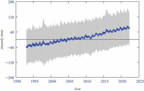
This study utilises GMSL data, shown in Figure 1,² which were generated using the Integrated Multi-Mission Ocean Altimeter Data for Climate Research (GSFC, 2022) for the period 1993–2022 consist of 1076 records (10-day average of global SA measurements). The updated time series combines Sea Surface Heights from TOPEX/Poseidon, Jason-1 and OSTM/Jason-2 with all biases and corrections applied and placed onto a georeferenced orbit. This creates a consistent data record throughout time, regardless of the instrument used. The GMSL time series is corrected for the effect of Global Isostatic Adjustment (GIA), (Beckley et al., 2016). The new time series, as compared to their previous version, include extended records and their standard deviations shown in Error: Reference source not found. Although the errors are nearly homogeneous, their magnitudes are relevant for accurate assessment of the investigated kinematic models and they are essential for the accuracy of the GMSL to be predicted.

Figure 1. Globally averaged sea level anomalies as observed by SA (blue) and their ±1σ uncertainties. The series consist of 1076 records during 1993–2022 (10-day averages).

3. Model I: kinematic model to represent the GMSL anomalies during 1993–2022 with a uniform global acceleration

A simple kinematic model was proposed and evaluated in recent studies (Ablain et al., 2019; Nerem et al., 2018; İ̇z & Shum, 2020). In this study, the model, Model I, is augmented by representations of annual and semi-annual GMSL variations,

(1) $h_t=h_{t_0}+\left(t-t_0\right)v_{t_0}+\frac{a}{2}{\left(t-t_0\right)}^2+\sum _m\left[{\alpha }_{m}sin\left(\frac{2\pi }{P_m}\left(t-t_0\right)\right)+{\gamma }_{m}cos\left(\frac{2\pi }{P_m}\left(t-t_0\right)\right)\right]+{\epsilon }_t$(1)

In this representation, $h_t$ denotes 10-day averaged global SA observations at epochs, $t=t_1\dots t_n,$ where n is the number of 10-day averages. The intercept $h_{t_0}$ is the reference height of the GMSL defined at the reference epoch $t_0=2005$ chosen to conform with the initial epoch of the previous studies. This designation is important since the estimated trend of the kinematic models is the initial velocity, $v_{t_0}$ and the trend/velocity changes over time in the presence of the uniform acceleration, a. The intercept $h_{t_0}$ is to be estimated together with the global initial velocity and uniform acceleration parameters. The model also includes the unknown coefficients of the annual and semi-annual harmonics denoted by ${\alpha }_m\wedge {\gamma }_m$ ($m=4$).

A competing kinematic model is discussed in the following section.

4. Model II: kinematic model to represent the GMSL anomalies during 1993–2022 with a 55.8 y periodicity

Sea level variations are multi-causal and occur at various time scales. There are several multidecadal effects whose presence were already established in TG series as discussed in the introduction section. For instance, a 60-year period in global sea level variations) was detected in TG records by Chambers et al. (2012). Haigh et al. (2011) reported a 59-year period generated by the interference of 8.85 y cycle of lunar perigee with 18.6 y nodal cycle at global scale. İ̇z (2014) also analysed 27 globally distributed long TG records and determined statistically significant signatures of sub- and super harmonics of lunar nodal tides and forced sea level variations including a long periodic subharmonic with a period 55.8 years as a global phenomenon. More recently, İ̇z and Shum (2020) demonstrated the presence of the same nodal subharmonic of period 55.8 y period in monthly SA record during 1993–2017.

Because of their similitudes in magnitudes, a uniform acceleration and the 55.8 y nodal subharmonic are collinear, hence they cannot be estimated simultaneously. To evaluate the effect of the 55.8 y periodicity at the global scale, the following offshoot of Equation (1)(1) $h_t=h_{t_0}+\left(t-t_0\right)v_{t_0}+\frac{a}{2}{\left(t-t_0\right)}^2+\sum _m\left[{\alpha }_{m}sin\left(\frac{2\pi }{P_m}\left(t-t_0\right)\right)+{\gamma }_{m}cos\left(\frac{2\pi }{P_m}\left(t-t_0\right)\right)\right]+{\epsilon }_t$(1) is now considered (Model II) in which the uniform acceleration is replaced with the 55.8 y periodicity, i.e.

(2) $h_t=h_{t_0}+\left(t-t_0\right)v_{t_0}+{\alpha }_{55.8}sin\left(\frac{2\pi }{P_{55.8}}\left(t-t_0\right)\right)+{\gamma }_{55.8}cos\left(\frac{2\pi }{P_{55.8}}\left(t-t_0\right)\right)+\sum _m\left[{\alpha }_{m}sin\left(\frac{2\pi }{P_m}\left(t-t_0\right)\right)+{\gamma }_{m}cos\left(\frac{2\pi }{P_m}\left(t-t_0\right)\right)\right]+{\epsilon }_t$(2)

The parameters of the Model II were already defined in Equation (1)(1) $h_t=h_{t_0}+\left(t-t_0\right)v_{t_0}+\frac{a}{2}{\left(t-t_0\right)}^2+\sum _m\left[{\alpha }_{m}sin\left(\frac{2\pi }{P_m}\left(t-t_0\right)\right)+{\gamma }_{m}cos\left(\frac{2\pi }{P_m}\left(t-t_0\right)\right)\right]+{\epsilon }_t$(1) together with their descriptions. Model I and Model II share the same statistical model discussed in the following section.

5. A new statistical model: first-order heterogeneously autoregressive disturbances

As reported in İ̇z and Shum (2020), the disturbance of the monthly and globally averaged GMSL disturbances exhibit first-order autoregressive disturbances with an estimated autocorrelation coefficient $\hat{\rho }=0.9$. The origin of the first-order autocorrelation can be attributed to large-scale events such as ENSO (Nerem et al., 2018), fusion of measurements from various SA altimetry missions, and smoothing and averaging SA data with 10-day intervals. In the earlier study by İ̇z and Shum (2020), the following statistical model has effectively eliminated the impact of the GMSL variations due to the AR(1) in estimating the parameters of the kinematics GMSL anomalies. The corresponding V/C matrix, denoted by $\mathrm{\Sigma }$, of the first-order autocorrelated disturbances, ${\epsilon }_t,$ is given by,

(3) $\mathrm{\Sigma }={\sigma }^2\cdot \left[\begin{array}{ccccc}1& \rho & {\rho }^2& \cdots & {\rho }^{t-1}\\ \rho & 1& \cdots & \cdots & {\rho }^{t-2}\\ ⋮& ⋮& ⋮& \ddots & ⋮\\ {\rho }^{T-1}& {\rho }^{T-2}& {\rho }^{T-3}& \cdots & 1\end{array}\right]$(3)

The autocorrelation decreases for increasing time lag because $\left|\rho \right|<1$. The correlation between two random variables ${\epsilon }_t\wedge {\epsilon }_{t-\tau }$ is ${\sigma }^2{\rho }^{\tau }$, where $\tau$ is the time lag with

(4) ${\epsilon }_t=\rho {\epsilon }_{t-1}+u_t,0\le \left|\rho \right|<1$(4)

The additive noise, $u_t,$ is assumed to be uniformly and identically distributed (iid), i.e. $u_{t}iid\left(0,{\sigma }_u^2\right)$, and ${\sigma }_u^2$ is the variance of the purely random variations (innovations).

Because the standard errors of the GMSL data are also provided for the new series (Error: Reference source not found) compared to the previous GMSL series, a different V/C matrix is required for proper statistical representation in this study. The following V/C matrix, abbreviated as ARH(1), is a first-order autocorrelation structure with heterogenous variances, ${\sigma }_1^2,\cdots ,{\sigma }_t^2$. The correlation between subsequent data is $\rho$, followed by ${\rho }^2$ for two records separated by a third, and so on giving way to the following first-order heterogeneously autocorrelated V/C matrix known as ARH(1),

(5) $\mathrm{\Sigma }=\left[\begin{array}{ccccc}{\sigma }_1^2& {\sigma }_2{\sigma }_1\rho & {\sigma }_3{\sigma }_1{\rho }^2& \cdots & {\sigma }_T{\sigma }_1{\rho }^{t-1}\\ {\sigma }_2{\sigma }_1\rho & {\sigma }_2^2& {\sigma }_3{\sigma }_2\rho & \cdots & {\sigma }_T{\sigma }_2{\rho }^{t-2}\\ ⋮& ⋮& ⋮& ⋮& ⋮\\ {\sigma }_T{\sigma }_1{\rho }^{t-1}& {\sigma }_T{\sigma }_2{\rho }^{t-2}& \cdots & \cdots & {\sigma }_t^2\end{array}\right]$(5)

The above structure can be derived by standardising the observation equations and restructuring the corresponding normal equations for a GLS solution.

In this model, an estimate of the first-order autocorrelation coefficient $\rho$ is calculated from the residuals of the OLS and used in the GLS solution in quantifying the V/C matrix for the SA measurements. The residuals of the GLS solution are then used to calculate a new ARH(1), which is then used in a GLS solution until there are no changes in the a posteriori variance of the unit weight (the standard error of the solution). Iterations result in an optimal ARH(1) correlation coefficient between adjacent disturbance terms to be used in the final GLS estimation.

In the following sections, ARH(1) statistical model is used to compare the above kinematics models, Model I and II.

6. Concurrent comparison of model I and model II

Table 1 lists pertinent solution parameters estimated using the GLS estimation for the Model I and Model II. The estimated velocity parameters are different, but the differences are not significant in magnitude. Because both models use the same data, the null hypotheses for the the differences are not meaningful. Nonetheless, the standard errors of the solutions (a posteriori variance of unit weights) are the same, so are their iteratively estimated autocorrelation coefficients of ARH(1). The estimates for the marginal harmonics shown in Table 2 are also practically the same in both models’ solutions. These outcomes suggest that both models are indistinguishable.

Table 2. The amplitudes of the estimated low frequency GMSL variations and their SE using model I and model II. All uncertainties are 1α. N/S: Not Significant ($\alpha =0.05$).

Solution	Component	Nodal mm/yr.	Solar mm/yr^2	Annual mm	Semi-annual mm
Model I	$\alpha$ γ	−1.60 ± 0.38 N/S	N/S 2.00 ± 0.34	−4.12 ± 0.31 −1.44 ± 0.30	N/S −1.60 ± 0.03
Model II	$\alpha$ γ	−1.69 ± 0.38 N/S	NS 1.90 ± 0.34	−4.12 ± 0.31 −1.45 ± 0.30	N/S −1.60 ± 0.03

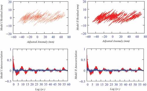
Figure 2 exhibits the time evolution of residuals of both kinematic model solutions, which are included here to consolidate the indifferences in the GLS estimates. Residuals of both model solutions are also indistinguishable from each other, as expected, and exhibit randomness. Meanwhile, plots of the residuals against the adjusted anomalies are shown in Figure 3 uncover episodic short lasting preponderant trends. The correlograms of both models residuals are similar and show that the residual unmodelled anomalies may be autocorrelated in nature other than ARH(1). The autocorrelations are strong with lags of up to 2–3 y. For longer lags, the autocorrelation coefficients are smaller in magnitude, yet they are episodic and persistent (autocorrelations in red). The random nature of the estimated random noise components, $u_t$ of the autocorrelated residuals, ${\epsilon }_t$, are confirmed through their autocorrelations (blue). The source of unmodelled short duration autocorrelations that are not accounted for ARH(1) could be of instrumental origin or atmospheric events at global scale and need to be investigated by the data centres for insight.

Figure 2. Residual properties of the model I (top) and model II solutions.

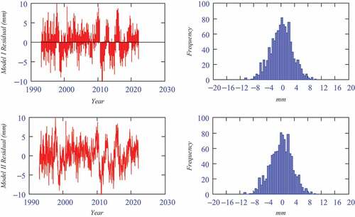
Figure 3. Residuals plotted against the adjusted GMSL anomalies to investigate unmodelled effects for model I and model II residuals (top two plots). Their correlelograms are displayed in the second row.

Some of the results presented above are redundant but they are included here to consolidate the outcome of the model solutions, which is not conclusive enough to validate one model over the other. Given the fact that both models represent the contemporaneous GMSL variations equally well, at this point one might ask, ‘what difference does it make to identify the correct model?’. This is the topic of the next section.

7. Prospective comparison of model I and model II

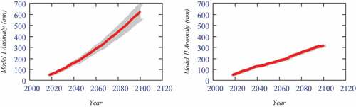
Predicted GMSL rise for the period 2022–2100 were carried out using both competing kinematic models. The underlying algorithm for the calculations was first introduced in sea level studies by İz et al., (2012), and further demonstrated and elaborated in İ̇z (2018). Compared to the traditional least squares prediction, which quantifies the expected values of the predicted anomalies, this approach provides the predictions for the actual values to be observed in the future with their prediction intervals (PI) instead of confidence intervals (CI). PIs are therefore better suited in sea level studies for risk assessments.

Figure 4 displays the predicted results for both models for the period 2022–2100. They are plotted on two separate graphs for clarity with the same vertical and horizontal axes for direct comparison. The plots exhibit stark differences between the predicted GMSL anomalies, and their uncertainties represented by their PIs with significance level α = 0.05.Model I predictions increases quadratically with larger and larger uncertainties because of the uniform acceleration generating a linearly increasing velocity, whereas Model II predictions are stable over time with visually imperceptible variations due to the nodal sub-harmonic with period 55.8 y with a constant trend/velocity. The predicted GMSL anomaly at 2100 by Model I is twice as large, compared to the Model II prediction.

Figure 4. Predicted GMSL rise for the period 2022–2100 for model I (left) and model II. Prediction intervals are in gray ($\alpha =0.05$).

8. Conclusion

Recent analyses of SA time series by Nerem et al. (2018), Ablain et al. (2019), and others reporting a uniform GMSL acceleration failed to recognise the epistemic uncertainty discussed in detail by İ̇z and Shum (2020). The current study revisited the topic in the light of newly available additional five years of global SA data and their standard errors. The outcome of the GLS solutions of two competing models did not find any statistical evidence favouring one model over the other either to alleviate the existing epistemic uncertainty. Nonetheless, through the comparison of the predictions carried out by the two competing kinematic models, this study demonstrated costly consequences of using a faulty model.

On one hand, a faulty Model I for prospective risk assessments would favour unnecessary interventions (mitigation instead of adaptation). Moreover, if Model II mirrors reality, then the outcome would introduce further ambiguity, raising the question about the missing impact of the anthropogenic contributions to the GMSL rise. Retrospective analysis of the TG measurements together with SA altimetry (İ̇z et al., 2018; İ̇z, 2017) may be instrumental to resolve this issue.

On the other hand, if the epistemic ambiguity is resolved in favour of Model II, then any attempt to reduce the impact of anthropogenic contributions to the global climate change would have little effect on GMSL rise and would necessitate interventions in favour of adaptation in decision making at global scale.

Acknowledgments

I would like to thank the three reviewers for their precious time in reviewing this paper and providing valuable comments. This research is partially supported by the Natural Science Foundation of China (Grant No. 41974040).

Disclosure statement

No potential conflict of interest was reported by the author.

Additional information

Funding

The work was supported by the Natural Science Foundation of China [41974040].

Notes

1. Note that, there other competing harmonics of luni-solar origin with long periods whose presence were quantified by Iz (2014) at globally distributed TG stations with long records. Their statistics, however, do not challenge the ambiguity of the uniform GMSL acceleration as effectively as 55.8 y period for the globally averaged SA records.

2. A detailed plot indicating mission periods is available at NASA’s PODAAC website https://podaac.jpl.nasa.gov/.

References

- Ablain, M., Meyssignac, B., Zawadzki, L., Jugier, R., Ribes, A., Spada, G., Benveniste, J., Cazenave, A., & Picot, N. (2019). Uncertainty in satellite estimate of global mean sea level changes, trend and acceleration. Earth System Science Data, 11(3), 1189–1202. https://doi.org/10.5194/essd-11-1189-2019
- Bâki Iz, H. B. ,. L., Berry, L., & Koch, M. (2012). Modeling regional sea level rise using local tide gauge data. Journal of Geodetic Science, Vol. 2(Issue 3), pp. pp. 188–1999. https://doi.org/10.2478/v10156-011-0039-2
- Beckley, B., Zelensky, N. P., Holmes, S. A., Lemoine, F. G., Ray, R. D., Mitchum, G. T., Desai, S., & Brown, S. T. (2016). Global mean sea level trend from integrated multi-mission ocean altimeters TOPEX/poseidon jason-1 and OSTM/Jason-2 version 4.2. Ver. 4.2. PO.DAAC, Dataset accessed [2022-06-22] at https://doi.org/10.5067/GMSLM-TJ142.
- Chambers, D. P., Merrifield, M. A., & Nerem, R. S. (2012). Is there a 60-year oscillation in global mean sea level? Geophysical Research Letters, 39(18), 18. https://doi.org/10.1029/2012GL052885
- Church, J. A., & White, N. J. (2006). A 20th century acceleration in global sea-level rise. Geophysical Research Letters, 33(1), L01602. https://doi.org/10.1029/2005GL024826
- Davis, J. L., & Vinogradova, N. T. (2017). Causes of accelerating sea level on the east coast of North America. Geophysical Research Letters, 44(10), 5133–5141. https://doi.org/10.1002/2017GL072845
- Dieng, H. B., Cazenave, A., Meyssignac, B., & Ablain, M. (2017). New estimate of the current rate of sea level rise from a sea level budget approach. Geophysical Research Letters, 44(8), 3744–3751. https://doi.org/10.1002/2017GL073308
- Douglas, B. C. (1992). Global sea level acceleration. Journal of Geophysical Research, 97(C8), 699–12706. https://doi.org/10.1029/92JC01133
- GSFC. (2022). Global mean sea level trend from integrated multi-mission ocean altimeters TOPEX/Poseidon, Jason-1, OSTM/Jason-2 version 4.2 Ver. 4.2 PO.DAAC. Available 22 June, 2022, from https://doi.org/10.5067/GMSLM-TJ42
- Haigh, I. D., Eliot, M., & Pattiaratchi, C. (2011). Global influences of the 18.61 year nodal cycle and 8.85 year cycle of lunar perigee on high tidal levels. Journal of Geophysical Research, 116(C6), C06025. https://doi.org/10.1029/2010JC006645
- Holgate, S. J., & Woodworth, P. L. (2004). Evidence for enhanced coastal sea level rise during the 1990s. Geophysical Research Letters, 31(7), L07305. https://doi.org/10.1029/2004GL019626
- Houston, J. R., & Dean, R. G. (2011). Sea-level acceleration based on U.S. Tide gauges and extensions of previous global-gauge analyses. Journal of Coastal Research, 27 (3) , 409–417.
- İ̇z, H. B. (2014). Sub and super harmonics of the lunar nodal tides and the solar radiative forcing in global sea level changes. Journal of Geodetic Science, 4 (1) , 150–165.
- İ̇z, H. B. (2017). Acceleration of the Global coastal sea level rise during the 20th century re-evaluated. Journal of Geodetic Science, 7(1)), 51–58. https://doi.org/10.1515/jogs-2017-0006
- İ̇z, H. B. (2018). Why and how to predict sea level changes at a tide gauge station with prediction intervals. Journal of Geodetic Science, 8(1), 121–129. https://doi.org/10.1515/jogs-2018-0012
- İ̇z, H. B. (2022). Low-frequency fluctuations in the yearly misclosures of the global mean sea level budget during 1900–2018. Journal of Geodetic Science, 12(1), 55–64. https://doi.org/10.1515/jogs-2022-0130
- İ̇z, H. B., & Shum, C. K. (2020). Certitude of a global sea level acceleration during the satellite altimeter era. Journal of Geodetic Science, 10(1), 29–40. https://doi.org/10.1515/jogs-2020-0101
- İ̇z, H. B., Shum, C. K., & Kuo, C. Y. (2018). Sea level accelerations at globally distributed tide gauge stations during the satellite altimetry era. Journal of Geodetic Science, 8(1), 130–135. https://doi.org/10.1515/jogs-2018-0013
- Jevrejeva, S., Grinsted, A., Moore, J. C., & Holgate, S. (2006). Nonlinear trends and multiyear cycles in sea level records. Journal of Geophysical Research, 111(C9), C09012. https://doi.org/10.1029/2005JC003229
- Keeling, C. D., & Whorf, T. P. (1997). Possible forcing of global temperature by the oceanic tides. Proceedings of the National Academy of Sciences, 94(16), 8321–8328. https://doi.org/10.1073/pnas.94.16.8321
- Munk, W., Dzieciuch, M., & Jayne, S. (2002). Millennial climate variability: Is there a tidal connection? Journal of Climate, 15(4), 370–385. https://doi.org/10.1175/1520-0442(2002)015<0370:MCVITA>2.0.CO;2
- Nerem, R. S., Beckley, B. D., Fasullo, J. T., Hamlington, B. D., Masters, D., & Mitchum, G. T. (2018). Climate-change–driven accelerated sea-level rise detected in the altimeter era. Proceedings of the National Academy of Sciences, 115(9), 1–4. https://doi.org/10.1073/pnas.1717312115
- Parker, B. B. (1992). Sea level as an indicator of climate and global change. Marine Technology Society Journal, 25(4 :13–24).
- IPCC. (2007). Summary for policymakersSolomon, S., Qin, D., Manning, M., Chen, Z., Marquis, M., Averyt, K. B., Tignor, M. and Miller, H. L. (Eds.), Climate change, 2007, the physical science basis. Contribution of working group I to the fourth assessment report of the intergovernmental panel on climate change. Cambridge University Press. 104 pp.
- Watson, P. J. (2011). Is there evidence of acceleration in mean sea level rise around mainland Australia? Journal of Coastal Research, 27(2), 368–377. https://doi.org/10.2112/JCOASTRES-D-10-00141.1
- Woodworth, P. L. (1990). A search for accelerations in records of European mean sea level. International Journal of Climatology, 10(2), 129–143. https://doi.org/10.1002/joc.3370100203
- Woodworth, P. L., White, N. J., Jevrejeva, S., Holgate, S. J., Church, J. A., & Gehrels, W. R. (2009). Evidence for the accelerations of sea level on multi-decade and century timescales. International Journal of Climatology, 29 (6) , 777–789.
- Yi, S., Sun, W., Heki, K., & Qian, A. (2015). An increase in the rate of global mean sea level rise since 2010. Geophysical Research Letters, 42(10), 1–9. https://doi.org/10.1002/2015GL063902
- Yndestad, H. (2006). The influence of the lunar nodal cycle on Arctic climate. ICES Journal of Marine Science, 63(3), 401–420. https://doi.org/10.1016/j.icesjms.2005.07.015
- Yndestad, H., Turrell, W. R., & Ozhigin, V., 2008, Lunar nodal tide effects on variability of sea level, temperature, and salinity in the faroe-shetland channel and the barents sea, deep sea research part I: Oceanographic research papers, vol. 55, issue 10, October 2008, pp 1201–1217.