The global change and response special project: using remote sensing data to monitor and invert key components in the cryosphere

ABSTRACT

It is critical to understand the mechanisms and impacts of global climate change in cryosphere and polar environment. Here we describe the design and progress of the remote sensing products we have developed to monitor these changes. We obtain datasets by combining multi-sensor remote sensing systems with field validation systems, and then develop a methodological system that combines multiple sources and calibration technologies to address the challenges of data heterogeneity in dynamically monitoring key parameters. This global change and response special project supported by the National Key Research and Development Program of China, named ‘observation and inversion of critical parameters of changes in the cryosphere and polar environment’, providing comprehensive records of essential elements of the cryosphere through long-term satellite records. The multi-team is completing the project and collecting data from multi-sensor to create remote sensing data products that include records of changes in the cryosphere, such as permafrost, glaciers, ice sheet mass balance, seasonal snow accumulation, sea ice, and albedo changes. Finally, the existing ground- and space-based observing system can be improved to provide dynamic monitoring of key parameters in the cryosphere and changes in the polar environment.

KEYWORDS:

• Cryosphere and Remote sensing observations
• Mountain glacier
• Permafrost
• Ice sheet
• Sea ice

1. Introduction

The driving mechanisms of global climate change requires understanding the complex and dynamic interactions between the Earth system and human beings (Qin et al., 2018; Xu et al., 2013). A critical link in these complex interactions is the cryosphere, an important part of the Earth system. It affects most latitudes, not just Greenland, Antarctica, and Qinghai-Tibet Plateau (QTP) regions. Changes in the cryosphere can seriously affect human life through events such as glacial lake outbursts, avalanches, short-term hazards, and sea level rise (SLR) as a long-term threat. The Intergovernmental Panel on Climate Change Sixth Assessment Report (IPCC AR6) on dynamic changes in the cryosphere shows that it has been shrinking rapidly over the past decade. The report details the changes in the components of the cryosphere, which include, but not limit to, polar ice sheets, mountain glaciers, permafrost, snow, and sea ice (Meredith et al., 2019).

The primary method for monitoring the major components of the cryosphere is using integrated, multi-source remote sensing techniques. A number of data products on key parameters in the cryosphere and on changes in the polar environment have recently been produced using observational technologies, including satellite remote sensing. These data products include glacier volume change and glacier mass balance based on InSAR, satellite laser altimetry, and optical remote sensing observations (Gardner et al., 2013; Raleigh et al., 2013). Global snow cover and snow water equivalent (Takala et al., 2011), sea ice (Fetterer et al., 2017; Parkinson and DiGirolamoa, 2021), and other remote sensing products are helping to advance complex numerical Earth system models and improve prediction accuracy. However, current global observations of key cryospheric parameters and data products are either spatially discontinuous or have coarse spatial resolution. The lack of good quality cryospheric data products, which are unable to adequately explain and understand the crucial dynamical processes in the polar regions, remains the main problem in global climate change research.

Here we discuss outcomes from the global change and response key special project supported by National Key Research and Development Program of China. We integrate multi-sensor remote sensing data with field investigations to understand climate change impacts, develop a system to fuse and calibrate data from multiple sources, create inversion methods and data products, and invert key cryospheric parameters. The multi-team completes the project and collects data from multi-sensor datasets to generate remote sensing data products records of changes in cryosphere. New objectives and techniques for creating data products of cryosphere are the main topics for this study. We address these issues under four main aspects: (1) multiscale observations and development of data products for key permafrost parameters; (2) observations and inversions related to global mass balance of mountain glaciers and other factors; (3) monitoring and inversion data products from satellite remote sensing related to key elements of ice sheets; and (4) an inversion method and product development related to sea ice changes. Our goal is to improve monitoring capabilities for ice sheets, mountain glaciers, permafrost, and sea ice by combining ground- and space-based observation systems and generating polar data products to achieve dynamic monitoring of the cryosphere.

2. Methods and data products in the cryosphere

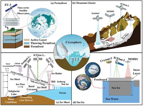
Data products from satellite remote sensing of key elements for the cryosphere include permafrost, mountain glaciers, ice sheets, and sea ice. We have developed some inversion methods that generate data products for monitoring key parameters. These data products could help test global change models and reduce uncertainties in climate change prediction models. In this study, we selected specific data products on permafrost, mountain glaciers, ice sheets, and sea ice we developed through this project are described in detail in Sections 2.1-2.4. Data products are available as relevant papers are published and all the other products have already been submitted to National Earth System Science Data Center (http://www.geodata.cn). However, due to the privacy policy of this project, some of the data products will open to the public one year after the project is completed (2024). Figure 1 shows an overview of the scope of this project and interactions between the satellite observation system and the cryosphere.

Figure 1. Overview of remote sensing techniques for monitoring ice dynamics in polar regions (modified from Lemke et al., 2007; Moon et al., 2018), including permafrost, mountain glaciers, ice sheets, ice shelves, and sea ice. (a) an example (ZY-3) of permafrost monitoring system components (active layer thickness, thawing permafrost distribution, and permafrost distribution) (modified from https://www.dawn.com/news/1433640) and other key elements in the study region; (b) mountain glacier showing monitoring elements and observation systems (modified from https://www.dawn.com/news/1433640); (c) sketch of an example scenario and key processes found in monitoring systems about outlet glaciers of Greenland and Antarctic ice sheets and ice shelves (ice disintegration due to rift changes) (modified from Dirscherl et al., 2020); (d) a schematic diagram of Arctic and Antarctic sea ice monitoring (sea ice thickness, albedo, area from satellite altimetry observation systems) (modified from Shepherd et al., 2018; Vaughan et al., 2013).

2.1. Permafrost

Permafrost covers about a quarter of the Northern Hemisphere (NH) and about 17% of the global exposed land surface (Biskaborn et al., 2019; Gruber, 2012). The thawing of frozen permafrost has been accelerated by global warming and has released soil organic carbon that contributes to global warming and provides a positive feedback loop (Biskaborn et al., 2019). Temperatures in perennial permafrost have increased, active layers have become thicker, and permafrost extent has decreased over the past decade (Meredith et al., 2019). By combining in situ measurements (such as station, borehole, soil temperature, moisture observation networks, geological field surveys, and UAV aerial surveys), multi-source remote sensing data, existing satellite remote sensing data products, and numerical models, we seek to develop global multi-year and seasonal permafrost distribution products to support the implementation of global change simulations (R. Li, Li, et al., 2021a).

We have developed global data on the freeze-thaw state of the soil and the thickness of the permafrost active layer from 2001 to 2020 based on a combination of ground-based and remote sensing observations of seasonal snow and permafrost. Zhao et al. (2017) found that there is a linear relationship between near-surface freeze/thaw and surface temperature in the QTP. We have further extended this linear correlation to global scale regions, observing a linear correlation between the freeze-thaw state function (25 km) and MODIS surface temperature (5 km) with an R-squared value greater than 0.7. Leveraging this relationship, we have generated 5 km spatial resolution soil freeze-thaw data products, and have produced global data products from 2002 to 2020. Our verification analysis indicates an accuracy greater than 90% (Liu et al., 2018). The product will help analyse other potential risks in the QTP and China-Pakistan Economic Corridor (CPEC) region, including infrastructure stability and vulnerability to thaw settlement. In situ soil temperature and soil moisture monitoring, remote sensing techniques, and permafrost field surveys were combined to improve the InSAR-based active layer thickness retrieval method in the permafrost regions (Chang et al., 2021). We have developed a model in the QTP permafrost regions to predict the spatial distribution of frozen ground temperature on a small scale. This model integrates in situ data by combining principal component analysis (PCA) and a geographically weighted regression model (GWR). The in situ data used for the model included 231 borehole temperature datasets with depths ranging from 0.2 m to 15 m, obtained along the Qinghai-Tibet Railway between May 2001 and Dec. 2001. We used this dataset to experimentally simulate and predict a three-dimensional spatial temperature field in a typical permafrost zone on the QTP (Zhao et al., 2021).

The data products for multi-year monitoring of permafrost in Antarctica, NH, and especially in the QTP, have high continuity and broad data coverage. We have collected previously published permafrost temperature monitoring data in the NH and Antarctica to expand the datasets’ time series. Each dataset contains between 15 and 25 monitoring points per hole along the railway and 15 monitoring points per hole in the vertical direction. The monitoring accuracy is high, with a monitoring frequency of 4 hours and an uncertainty of 0.5°C. Figure 2 shows the distributions of the new in situ site stations. Using permafrost drilling to determine the characteristics, homogenisation, and quality control of existing permafrost temperature observations, and upscaling of point observations to obtain permafrost temperature grid data for the NH and Antarctica, we have obtained accurate multi-year permafrost temperatures from 2001 to 2020 based on the station data for Antarctica and the NH, including the QTP. Table 1 provides comprehensive details on the permafrost data products.

Figure 2. The distribution of multi-year permafrost geothermal observation sites along the Qinghai-Tibet railway on the QTP from December 2018 to January 2021. The background depicts the permafrost distribution on the Tibetan Plateau, as identified by Zou et al. (2017).

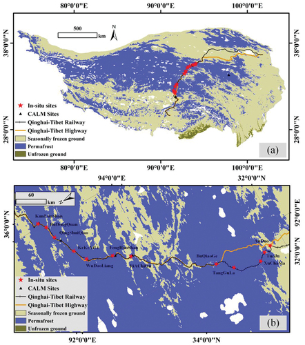
Table 1. List of permafrost products characteristics.

Products	Time SPAN	Spatial and Temporal Resolution	Sensors Datasets	Data Accessibility
Soil Freezing and Thawing*	2002–2020	5 km (Daily)	MODIS, AMSR-E, AMSR2	http://www.geodata.cn
Permafrost Active Layer Thickness*	2001–2020	1 km (Yearly)	Envisat, Sentinal-1, MODIS	http://www.geodata.cn
Permafrost Surface Deformation*	2001–2020	5 m (12-days)	ENVISAT, Sentinel-1, ALOS-PALSAR, TerraSAR-X, COSMO-SkyMed	http://www.geodata.cn
Multi-year Permafrost Ground Temperature Monitoring Data*	2018–2020	Point Scale datasets/-	In situ measurements	http://www.geodata.cn

*These data products will release in April 2024.

2.2. Mountain glaciers

The impact of climate change on global SLR depends strongly on the area and thickness of glaciers in polar regions (Millan et al., 2022). Over the past 60 years, mountain glaciers melting may have accounted for 25% to 30% of the total observed SLR (Watson et al., 2015), a contribution to global SLR comparable to that of Greenland and much higher than that of Antarctica (IMBIE., 2018; Khan et al., 2015; Zemp et al., 2019). According to recent studies, global mountain glacier mass loss has accelerated over the past 20 years (Hugonnet et al., 2021). Therefore, it is essential to investigate data products on key elements of mountain glaciers, such as glacier inventory and changes in thickness. In this study, we conducted a cross-thematic investigation of factors affecting the calculation of mountain glaciers mass balance.

We have developed inversion techniques for essential elements of mountain glaciers and methodological systems for inversion of key elements such as topography, ice thickness variability, albedo, ground-based observational controls, basin-scale glacier mass variability, and global mountain glaciers mass balance. We combined albedo inversion models, in situ measurements, unmanned aerial vehicle (UAV) data, multi-sensor satellite data (MODIS, TanDEM-X, ICESat-1/2, CryoSat-2, ZY-3), ground-based LiDAR, InSAR, GPS, and ice radar to produce the high spatial and temporal resolution products of mountain glaciers mass balance and evaluate their accuracy.

In the context of the Third Polar Region (TPR) or high-mountain Asia region, existing glacier inventories exhibit substantial spatial coverage and data quality heterogeneity. Therefore, a rigorous assessment of data quality is essential to facilitate the selection of an appropriate glacier inventory for specific research applications. He and Zhou (2022b, 2022a) evaluated eight glacier inventories (GGI18, GGI-2, HKHGI, WHGI, KPGI, PGI-2, SETPGI, and TPGI) to determine the accuracy of different glacier inventories by using the analytical hierarchy process on the TPR. Merging the products of the eight glacier inventories resulted in a new glacier inventory with high quality for the entire TPR. This newly developed glacier catalogue is expected to meet the needs of a diverse range of researchers by providing comprehensive information on specific parameters from a single inventory. Glacier inventory products for the mountain glaciers and ice caps in Greenland and Antarctica were generated using semi-automatic glacier mapping based on threshold band ratios (Paul & Kaab, 2005; Paul et al., 2002, 2016) of multispectral satellite data, which were then manually corrected for ice contours in misclassified areas to produce a glacier inventory dataset for Greenland from 1990 to 2020. The Antarctic glacier boundary was extracted by manually digitising the imagery. A watershed algorithm based on a high-precision DEM (Reference Elevation Model of Antarctica, REMA) (Howat et al., 2019) was used to update the watershed delineation of mountain glaciers for the Antarctic region glacier inventory from 2000 to 2020.

Ice velocity data are important to study glacier dynamics and to improve glacier models. Based on the method from Shen et al (2018, 2021). we generated a high-resolution 100-m ice velocity data product in the mountain glacier regions, the highest-resolution annual ice velocity data product for mountain glaciers to date, which is comparable to other advanced international products.

Analysis of long-term, reliable albedo products will contribute to a better understanding of feedback between the Earth surface and global climate change. For mountain glacier albedo, we have adopted different processing strategies based on regional features to extract the albedo of mountain glaciers in a specific area (Tian & Liu, 2021). The occurrence of cloud cover occlusion poses a significant challenge in acquiring complete snow albedo data. Box et al. (2017) proposed a technique that integrates smoothing and gap-filling effects into MOD10A1 albedo images to fill in the gaps. Tian et al. (2019) further enhanced this approach by incorporating a cubic spline interpolation procedure. The accuracy of this modified technique was verified to be RMSE < 0.05 for the Greenland Ice Sheet. Building upon this, Ye and Tian (2022) utilised a similar approach by combining Google Earth Engine remote sensing big earth data cloud platform based on MOD10A1 version 6 snow albedo to obtain temporally continuous data in Alaska and Canadian Arctic regions. The regression analysis results on data acquired from White Glacier in the Canadian Arctic Archipelago indicated that the gap-free data effectively reflect changes in mass balance (Ye & Tian, 2022).

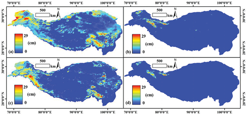
Yan et al. (2022) downscale snow depth data from the QTP using a spatiotemporal subpixel decomposition algorithm to obtain snow depth data on a daily scale of 0.05° and improve understanding of the spatiotemporal variability of snow depth in the QTP. The snow depth decay model was used to complement the microwave-assisted inversion of snow depth values in areas of thin snow. The satellite remote sensing products for snow depths are shown in Figure 3. To obtain snow water equivalent data, snow depth is converted to snow water equivalent using snow density (Yan & Zhang, 2022). In this study, we develop a new snow albedo data product by combining existing products and other supporting information. We fuse 0.1° of the ERA surface albedo data to produce a 0.05° snow albedo data product with high spatial resolution. Under clear sky conditions, snow and ice data fusion data products of MODIS Terra (MOD10A1), MODIS Aqua (MYD10A1), and IMS (Interactive Multisensor Snow and Ice Mapping System) are significantly more accurate than the MODIS Terra and Aqua 8-day seasonal snow distribution data products, and the overall accuracy of the data product is comparable to that of the MODIS Terra 8-day product.

Figure 3. A daily spatial pattern of the 0.05° snow depth product (Yan et al., 2022) over the QTP in (a) SD_2008031; (b) SD_2008200; (c) SD_2018031; and (d) SD_2018200, respectively. The naming rule is “SD_yyyyddd”, where “SD” is snow depth, “yyyy” is year, and “ddd” is Julian day.

Basin-scale mass loss was determined using the Tongji-GRACE-2018 (Chen et al., 2019) and Tongji-RegGrace2019 (Chen et al., 2021) models with GRACE satellite data published on the Global Gravity Field Model Center website (http://icgem.gfz-potsdam.de/series). The study of mountain glacier’s mass balance is of great importance. However, gravity methods can only accurately estimate total mass loss and cannot analyse mass trends for specific glaciers due to its coarse resolution. Therefore, to improve the accuracy and reliability of mountain glacier terrain reconstruction, ice thickness change detection, and mass balance data products, a multi-source DEM-based mass balance geodetic estimation method was developed (Liu et al., 2016, 2019, 2020). Glacier mass balance records on the QTP are limited due to the region’s harsh weather conditions and mountainous topography, which have hindered our understanding of glacier melting and its response to climate change. To address this issue, Zhang et al. (2018) developed a statistical and analytical model for estimating glacier albedo-mass balance, a glacier albedo-based method for annual seasonal mass balance estimation was proposed (Zhang et al., 2018). The study found a significant linear correlation between annual minimum mean glacier albedo values and annual mass balance measurements at Xiao Dongkemadi glacier (R² = 0.941, P < 0.001). Furthermore, the study reconstructed a 17-year annual mass balance series for the Xiao Dongkemadi glacier, each glacier of the Geladandong mountain region and the Purogangri ice cap for the first time. The proposed method was validated using geodetic measurements, which indicated that the albedo-based process is capable of estimating the mass balance of QTP glaciers. These findings provide valuable insights into the mass balance records of glaciers on the QTP (Zhang et al., 2018). Details of the mountain glacier data products are listed in Table 2, including the parameters of the products, time span, spatial and temporal resolution, and data source.

Table 2. List of mountain glacier product characteristics.

Products	Time Span	Spatial and Temporal Resolution	Sensors Datasets	Data Accessibility
Glacier Inventory	2001–2020	-/Multi-yearly	Landsat	https://doi.org/10.11888/Cryos.tpdc.272302 https://cstr.cn/18406.11.Cryos.tpdc.272302
Glacier Inventory*	1990–2020	100 m/ Multi-yearly	Landsat 7–8	http://www.geodata.cn
Ice Velocity*	2001–2020	100 m/Multi-yearly	Landsat 7–8	http://www.geodata.cn
Albedo*	2017–2020	300 m Monthly	Sentinel-3	http://www.geodata.cn
	2001–2020	500 m Monthly	MODIS	http://www.geodata.cn
Snow Depth Product	2001–2020	0.05° 8-days	MODIS	https://doi.org/10.11888/Snow.tpdc.271743
Snow Cover Extent*	2001–2020	500 m 8-days	MODIS	http://www.geodata.cn
Snow Water Equivalent	2001–2020	5 km Daily	SSMI、AMSRE and AMSR2	https://doi.org/10.11888/Cryos.tpdc.272289 https://doi.org/CSTR:18406.11.Cryos.tpdc.272289
Snow Water Equivalent*	2001–2018	1 km Daily	MODIS	http://www.geodata.cn
Snow albedo*	2001–2020	1 km 8-days	MODIS	http://www.geodata.cn
Gravity Variation in Basin-scale mass balance*	2002–2020	1 km 8-days	GRACE, GRACE Follow-on	http://www.geodata.cn
Mountain Glacier mass balance*	2001–2020	100 m Multi-yearly	ZY-3 DEM, SRTM DEM, and TDX	http://www.geodata.cn
	2001–2013	30 m Multi-yearly	SRTM and TDX Globe DEM	http://www.geodata.cn
	2001–2013	100 m Multi-yearly	Multi-source and TDX Global DEM	http://www.geodata.cn

*These data products will release in April 2024.

2.3. Ice sheets

The pressing issue of ice sheet mass change and its implications for current and future sea level rise has garnered significant attention from the scientific community (Shepherd et al., 2012, 2018; Smith et al., 2020). The immense sea level equivalent of the Antarctic and Greenland Ice Sheets, with 7.2 m and 57.9 m, respectively (Aschwanden et al., 2019; Morlighem et al., 2020; Rignot et al., 2008). The Antarctic Ice Sheet experiences mass loss primarily through basal melting and ice calving, accounting for approximately 50% of the total loss (Liu et al., 2015; Rignot et al., 2013). Meanwhile, the Greenland Ice Sheet’s mass loss is attributed to three primary mechanisms: surface melt runoff, constituting the majority at 50%-65%; tidal glaciers and icebergs calving have the same amount of contribution, about 15%-25% (Smith et al., 2020). Nowadays, satellite altimetry (e.g. CryoSat-2, ICESat-2), optical imagery (e.g. DISP, Landsat, Worldview, and ZY-3), and radar echo-sounding data have been used to generate data products for the ice sheets and ice shelves.

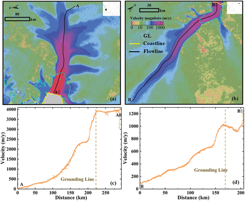
To generate historical ice velocity data, Li et al. (2017) developed methods based on parallax decomposition, hierarchical matching, and satellite image matching (Ye et al., 2017), and they also proposed a method to correct overestimates in historical velocity maps (Li et al., 2022). These methods were then used to produce ice velocity maps for Greenland and Antarctica from the 1960s to the 1980s (Luo et al., 2021; Yu et al., 2022; Feng et al., 2022). Accurate estimation of early mass losses requires preliminary analysis of ice velocity, spatial acceleration, and surface slope on the distribution of reconstructed historical ice velocity map corrections and their potential influence on the East Antarctic Ice Sheet (EAIS) mass balance assessment (Ge et al., 2022). In recent years, new opportunities and changes in the inversion of data products have emerged due to the increasing availability of remote sensing data in polar regions. To produce high-resolution ice velocity mapping products in Antarctica from 2013 to 2019, Shen et al. (2018) developed the nonlocal mean filtering method. This velocity map has higher spatial resolution compared to multi-year InSAR data products (Rignot et al., 2011b) and the current ice flow product ITS-LIVE (Gardner et al., 2018). It improves the signal-to-noise ratio of the product while providing minimal loss of resolution. This makes it the most comprehensive and highest-resolution annual product for Antarctica (Shen et al., 2018, 2021). Figure 4 shows velocity data products for the selected Antarctic ice shelf sections from this product (Shen et al., 2018, 2021).

Figure 4. Ice velocity mapping and profile along the central flowlines (AA’, BB’) for (a) and (c) Pine Island Glacier and Rayner Glacier (b) and (d) from Shen et al (2018, 2021). Pine Island Glacier: 2013–2016; Rayner Glacier: 2013–2019.

Daily albedo for the Greenland data product was filtered using the 11-day statistical method proposed by Box et al. (2017), which also addresses the problem of data gaps in regions with long-term cloud cover, such as the north-central Greenland sector. We use the cubic spline function (Tian et al., 2019) to fill the gaps and create a temporally and spatially continuous albedo reanalysis data product for Greenland. The accuracy of the data products was validated using ground-observation data from the Programme for Monitoring of the Greenland Ice Sheet (PROMICE) provided by the Geological Survey of Denmark and Greenland (GEUS). Results of the validation showed that the reanalysed albedo data products were temporally and spatially continuous, with an RMSE under 0.05, as described in Tian et al. (2019). We cross-validated and reanalysed the MCDA3V006 albedo product with ground-based meteorological station data and other albedo products to fill the gaps and produce gapless 500 m resolution albedo data products for Antarctica. To address the issue of prolonged and widespread missing data for the MCD43A3V006 albedo data products in Antarctica, we have proposed a workflow building a multiple linear regression model between ERA5 meteorological data and MCD43A3V006 albedo, which enables the calculation of albedo for vacant regions using long time series of vacancy-free ERA5 meteorological data. A multiple linear regression model was used to establish regression relationships between the MCDA3V006 albedo product and the ERA5 meteorological factors. The albedo of the vacant region was calculated using long time series of vacancy-free ERA5 meteorological data.

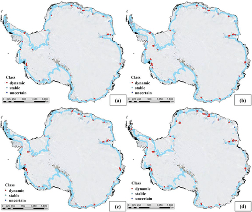
Because grounding lines (GLs) are a crucial indication of ice sheet instability, their locations are essential for ice velocity measurement and analysis (Friedl et al., 2020). To systematically assess the accuracy of the five major existing data products of GL, MOA GL 2004 (Haran et al., 2005; Haran et al., 2014), MOA GL 2009 (Haran et al., 2014), ASAID GL (Bindschadler et al., 2011), ICESat Grounding Zone (GZ) (Brunt et al., 2010), and InSAR GL (Rignot et al., 2011a), Li, Lv, et al. (2021b) proposed a new assessment strategy and process that conducted a comprehensive assessment of GL from 2002 to 2009. Based on the assessment result, we updated the GL data products shown in Figure 5. In addition, we developed a fusion algorithm based on the analysis of slope and surface curvature using the CryoSat-2 altimetry data and Landsat-8 optical data to extract the 2017 GL for the Amery Ice Shelf in East Antarctica (Li et al., 2020). Second, Xie et al. (2016) proposed an improved plane-fitting model using Landsat 8 OLI and ICESat data to eliminate slope-induced errors in the ICESat GL extraction procedure. The manually digitised and extracted Landsat 8 GL data were then subjected to a least squares model to correct the ICESat GL position and produce an accurate GL data product for the Amery sector.

Figure 5. Antarctica GL update products, (a) MOA 2004 GL update results; (b) MOA 2009 GL update results; (c) ASAID GL update results; (d) InSAR GL update results.

Analysis of ice shelf and 3D ice rift parameters and identification of ice shelf calving events have been performed using satellite remote sensing data from various sources (Li et al., 2019; Xiao et al., 2017; Zhao et al., 2022). A long-term time series of remote sensing data is used to identify the distribution and processes of marine ice sheet change and potentially accelerating trends in Greenland and Antarctic mass loss and their contribution to SLR. Basal channels and subglacial water highly influence ice sheet dynamics and stability. Based on satellite altimetry, we have developed methods for detecting subglacial water (Wang et al., 2021) and the inversion of its activities (Fan et al., 2022). Table 3 shows the ice sheet data products in detail.

Table 3. List of characteristics of ice sheet and ice shelve element products.

Products	Time Span	Spatial and Temporal Resolution	Sensors Datasets	Data Accessibility
Ice Velocity Mapping*	1963–1989	500 m/ Multi-yearly	DISP, Landsat-1/2/4/5	http://www.geodata.cn
Ice Velocity Mapping	2013–2019	100 m/ Multi-yearly	Landsat-7/8	https://doi.pangaea.de/10.1594/PANGAEA.908845 https://data.tpdc.ac.cn
Albedo*	2000–2020	500 m/Daily	MODIS	http://www.geodata.cn
Grounding Line*	2002–2009	-/Multi-yearly	Multi-Source	http://www.geodata.cn
Mass Balance*	1990–2020	500 m/ Multi-yearly	Multi-Source	http://www.geodata.cn

*These data products will release in April 2024.

2.4. Sea ice

Another important indicator of global climate change is the extent of sea ice in the polar regions. Sea ice covers about 7% of the Earth’s surface and about 12% of the world’s oceans (Weeks, 2010). Observations of long-term interannual and seasonal sea ice patterns are based on multiple satellite remote sensing sources. It is critical to investigate the possible coupled responses of the Arctic and Antarctic sea ice and their impacts on global climate change. We have developed satellite remote sensing data products for Arctic and Antarctic sea ice parameters such as area, spatial distribution, thickness, albedo, and concentration from 2001 to 2020.

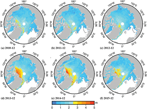
To increase the spatial resolution of passive microwave sea ice data, Liu et al. (2022) proposed a novel multi-image super-resolution (MISR) network, the progressive multiscale deformable residual network (PMDRnet), based on the properties of passive microwave imagery and sea ice motion. The state-of-the-art PMDRnet method outperforms other MISR methods. It can produce fine-scale sea ice area and margin line products, and high-resolution sea ice margins with enhanced texture features and sharper sea ice extent products (Liu et al., 2022). Radar penetration reflection coefficients are added, and freeboard thickness is optimised using altimetry data from ERS, Operation IceBridge, Envisat, CryoSat-2, ICESat, and ICESat-2, increasing the accuracy of thickness extraction (Xiao et al., 2021; Zhang et al., 2021, 2022). Using sea ice concentration, snow thickness, and density as unknown parameters and the least squares method for iterative calculation, a method for estimating sea ice thickness based on CryoSat-2 data was proposed. This method (1) does not follow the conventional technique of using empirical values, (2) reduces the number of input parameters, and (3) improves the reliability of the calculated sea ice thickness. After preprocessing and residual elevation filtering, the ICESat-2 data are used to calculate sea ice freeboard and local sea surface height. The combination of ICESat-2 and CryoSat-2 satellite altimetry data results in the inversion of snow thickness, which reduces the uncertainty in the sea ice freeboard extraction. Figure 6 shows the sea ice thickness results in the Arctic regions in December from 2010 to 2015 (Xiao et al., 2020; Zhang et al., 2021).

Figure 6. Arctic sea ice thickness data products in December from 2010 to 2015.

To generate sea ice albedo products of the Arctic (500 m) and Antarctica (1 km) with a temporal resolution of 10 days, we use an iteration procedure with MODIS (2000–2020) and VIIRS (2012–2020) data, respectively. For 2000–2011, we also used a spatial-temporal data fusion method (Spatial and Temporal Nonlocal Filter Based Fusion Model, STNLFFM) proposed by Cheng et al. (2017) to generate the Antarctic albedo products from appendix datasets. Passive microwave sea ice concentration products covering the Arctic and Antarctica were generated from SSMI (2001–2002), AMSR-E (2002–2011), and AMSR-2 (2012–2020), respectively. Using remote sensing data from Sentinel-1 SAR and Advanced Microwave Scanning Radiometer 2 (AMSR2), ship-based observations, and other data products, we generated sea ice concentration, extent, and thickness products for the research vessel Xue Long to plan routes along the cruise passage during the Arctic and Antarctic expeditions. During the Arctic summer, accuracy is low because optical images are affected by the atmosphere and other factors. By combining with data from SAR, the quality and reliability of the data can be improved. The 38th Chinese Antarctic Scientific Expedition (2021–2022) and the 11th Chinese Arctic Scientific Expedition (2020) used in situ measurements to verify our sea ice data products in the Antarctica and Arctic. These serve as the basis for forecasting sea ice conditions and as useful reference information for positioning and deploying/recovering the submerged marine buoys. The details of the sea ice data products in this study are given in Table 4.

Table 4. List of Arctic and Antarctic sea ice element product characteristics.

Products	Time Span	Spatial and Temporal Resolution	Sensors Datasets	Data Accessibility
Sea Ice Edge, Area, Extent*	2001–2020	1.5625 km (Monthly)	SSMI, MISR, AMSR2	http://www.geodata.cn
Sea Ice Thickness*	2001–2021	5 km (Monthly)	ERS-2, Envisat, ICESat, CryoSat-2, Operation IceBridge, and ICESat-2	http://www.geodata.cn
Sea Ice Albedo*	2000–2020	500m;1 km (10-days)	MODIS、AVHRR	http://www.geodata.cn
Sea Ice Concentration*	2000–2020	1km; 2 km; 5 km (Daily)	SSMI, AMSE-E, and AMSR-2	http://www.geodata.cn

*These data products will release in April 2024.

Sea ice data assimilation links sea ice data products and numerical forecast models. An optimal interpolation (OI) algorithm is employed to assimilate satellite-observed sea ice concentration (SIC) into a global 1/10° surface wave-tide-circulation coupled ocean forecast system (FIO-COM10, Sun et al., 2020) to improve its sea ice forecast capabilities. Model resolution and the physical processes included are the two most influential factors in determining the realism or performance of ocean simulation models. Xiao et al. (2023) developed the FIO-COM32 full spherical wave-tide circulation coupled ocean model. It has a 1/32° resolution and an increase in horizontal model resolution from 1/10° to 1/32°. The new model significantly improves simulations of surface EKE, Kuroshio, Gulf Stream main paths, and global tides (FIO-COM32, Xiao et al., 2023). The inclusion of sea ice data assimilation can effectively reduce the large biases in sea ice concentration. The most significant improvement is observed in the marginal ice zones, and the improvement is more pronounced in areas with relatively low SIC. The real-time forecast results indicate that the SIC data assimilation profoundly improves the forecast capability of polar sea ice in the global ocean forecast system.

3. Discussion and conclusion

This study describes the design and progress of integrated observation and monitoring systems for the cryosphere and polar environment based on a combination of satellite- and ground-based observation technologies. We continue to develop data products such as permafrost active layer thickness, glacier inventory, ice velocity, ice sheet mass balance, and sea ice thickness to achieve dynamic monitoring of the global climate change. This will improve our understanding of the interaction mechanisms between critical parameters of the cryosphere and global climate change.

First, we attempt to build a dynamic observation system for the polar regions to improve current cross-platform observation systems (space- and ground-based platforms) and address critical scientific questions about global climate change. To achieve synergistic observations and model inversions, this study combines multiple long-term observation facilities (e.g. ground- and sea-based platforms, Snow-Eagle 601 fixed-wing aircraft, and UAVs) during the Chinese polar expeditions. Our ability to understand critical processes and coupled response mechanisms in the cryosphere has been enabled by multi-platform collaborative observational networks and data products for a better understanding of global climate change.

Second, the data products of this study could advance climate change research by: (1) developing new products on the components of the cryosphere (e.g. soil freeze-thaw state data product for the CPEC to address concerns about the environmentally friendly and sustainable implementation of the ‘One Belt, One Road’ project); (2) investigating the coupled responses of Arctic and Antarctic sea ice and their impacts on global climate change, and analysing their spatial and temporal variability to improve model prediction capabilities and optimise shipping routes; (3) analysing the spatial and temporal variability of sea ice data products in polar regions, including sea ice thickness, extent, albedo and concentration; and (4) production of ice velocity maps in Antarctica and Greenland using historical imagery from the 1960s to 1980s and combining the input-output method for calculating ice sheet mass balance to reduce its estimation uncertainty and to improve the predictive accuracy of the contribution to global SLR.

Finally, these data products will help reduce uncertainties in global glaciers’ mass balance analysis. These three data products will fill research gaps in the polar regions on a global scale: (1) a regional permafrost active layer thickness inversion product for the, based on the fusion of ground-based and InSAR remote sensing data; (2) multi-year and seasonal mapping of permafrost distribution in QTP; and (3) ice velocity mapping products for Antarctica and Greenland between 1963 and 1989.

With new data to construct a longer time series dataset, we will continue to focus on data products from remote sensing in the cryosphere. We will improve the observation system for in situ measurements to obtain a higher density of long-term observation series, increase the accuracy and precision of the data products, and reduce uncertainties. We also expect these data products to receive user feedbacks after they are all released in the near future for further improvements. We aim to enhance our ability to produce high-precision data products from satellite remote sensing in the cryosphere.

Acknowledgments

We greatly acknowledge the use of imagery from ESA (available via https://ecoat.esa.int/ and http://search.saf.alaska.edu), USGS (available via https://earthexplorer.usgs.gov/), and JPL for providing us the GRACE data (available via https://podaac.jpl.nasa.gov/), ZY-3 satellite data images (accessed to http://www.lasac.cn/).

Disclosure statement

No potential conflict of interest was reported by the author(s).

Data availability statement

The 0.05° snow depth product is available from the National Tibetan Plateau Data Center (https://doi.org/10.11888/Snow.tpdc.271743). Data products of high-quality Antarctic-wide ice velocity maps and their corresponding uncertainty estimates are freely available from the Data Publisher for Earth & Environmental Science (https://doi.pangaea.de/10.1594/PANGAEA.908845) and the National Tibetan Plateau Data Center (https://data.tpdc.ac.cn). Assessment of Glacier Inventories for the Third Pole Region (1990–2015) is freely available from the National Tibetan Plateau Data Center (http://data.tpdc.ac.cn/zh-hans/download/d31370e1-089e-40e1-8b39-0687ba84a84c/). The daily 0.01°Snow water equivalent datasets for Tibetan Plateau (2000–2018) (https://doi.org/10.11888/Cryos.tpdc.272289 or https://doi.org/CSTR/18406.11.Cryos.tpdc.272289). We will submit the other remote sensing data products in the polar regions to the National Earth System Science Data Center, National Science & Technology Infrastructure of China (http://www.geodata.cn).

Additional information

Funding

This study was supported by the National Key Research and Development Program of China (No.2017YFA0603100).

References

- Aschwanden, A., Fahnestock, M. A., Truffer, M., Brinkerhoff, D. J., Hock, R., Khroulev, C., Mottram, R., & Khan, S. A. (2019). Contribution of the Greenland ice sheet to sea level over the next millennium. Science Advances, 5(6), eaav9396. https://doi.org/10.1126/sciadv.aav9396
- Bindschadler, R., Choi, H., Wichlacz, A., Bingham, R., Bohlander, J., Brunt, K., Corr, H., Drews, R., Fricker, H., Hall, M., Hindmarsh, R., Kohler, J., Padman, L., Rack, W., Rotschky, G., Urbini, S., Vornberger, P., & Young, N. (2011). Getting around Antarctica: New high-resolution mappings of the grounded and freely-floating boundaries of the Antarctic ice sheet created for the international polar year. The Cryosphere, 5(3), 569–588. https://doi.org/10.5194/tc-5-569-2011
- Biskaborn, B. K., Smith, S. L., Noetzli, J., Matthes, H., Vieira, G., Streletskiy, D. A., Schoeneich, P., Romanovsky, V. E., Lewkowicz, A. G., Abramov, A., Allard, M., Boike, J., Cable, W. L., Christiansen, H. H., Delaloye, R., Diekmann, B., Drozdov, D., Etzelmüller, B. … Lantuit, H. (2019). Permafrost is warming at a global scale. Nature Communications, 10(1), 264. https://doi.org/10.1038/s41467-018-08240-4
- Box, J. E., van as, D., & Steffen, K. (2017). Greenland, Canadian and Icelandic land ice albedo grids (2000-2016). Geological Survey of Denmark and Greenland Bulletin, 38, 53–56. https://doi.org/10.34194/geusb.v38.4414
- Brunt, K., Fricker, H., O’Neel, S., & Padman, L. (2010). Icesat-derived grounding zone for Antarctic ice shelves. U.S. Antarctic program (USAP) data center. Lasted Retrieved September , 2022. https://doi.org/10.7265/N5CF9N19
- Chang, T., Han, J., Li, Z., Wen, Y., Hao, T., Lu, P., & Li, R. (2021). Active layer thickness retrieval over the Qinghai-Tibeat plateau from 2000 to 2020 based on InSAR-measured subsidence and multi-layer soil moisture. The International Archives of the Photogrammetry, Remote Sensing and Spatial Information Sciences, XLIII-B3-2021, 437–442. https://doi.org/10.5194/isprs-archives-XLIII-B3-2021-437-2021
- Cheng, Q., Liu, H., Shen, H., Wu, P., & Zhang, L. (2017). A Spatial and temporal nonlocal filter-based data fusion method. IEEE Transactions on Geoscience and Remote Sensing, 55(8), 4476–4488. https://doi.org/10.1109/tgrs.2017.2692802
- Chen, Q., Shen, Y., Chen, W., Francis, O., Zhang, X., Chen, Q., Li, W., & Chen, T. (2019). An optimized short‐arc approach: Methodology and application to develop refined time series of Tongji‐Grace2018 GRACE monthly solutions. Journal of Geophysical Research: Solid Earth, 124(6), 6010–6038. https://doi.org/10.1029/2018JB016596
- Chen, Q., Shen, Y., Kusche, J., Chen, W., Chen, T., & Zhang, X. (2021). High-resolution GRACE monthly spherical harmonic solutions. Journal of Geophysical Research: Solid Earth, 126(1), e2019JB018892. https://doi.org/10.1029/2019JB018892
- Dirscherl, M., Dietz, A. J., Dech, S., & Kuenzer, C. (2020). Remote sensing of ice motion in Antarctica – a review. Remote Sensing of Environment, 237, 111595. https://doi.org/10.1016/j.rse.2019.111595
- Fan, Y., Hao, W., Zhang, B., Chao, M., Gao, S., Shen, X., & Li, F. (2022). Monitoring the hydrological activities of Antarctic subglacial lakes using CryoSat-2 and ICESat-2 altimetry data. Remote Sensing, 14(4), 898. https://doi.org/10.3390/rs14040898
- Feng, T., Li, Y., Wang, K., Qiao, G., Cheng, Y., Yuan, X., Li, R., & Li, R. (2022). A hierarchical network densification approach for reconstruction of historical ice velocity fields in East Antarctica. Journal of Glaciology, 69(274), 1–20. https://doi.org/10.1017/jog.2022.58
- Fetterer, F., Knowles, K., Meier, W. N., Savoie, M., & Windnagel, A. K. (2017). Sea Ice Index, Version 3. National Snow and Ice Data Center. Indicate subset used. Updated daily. https://doi.org/10.7265/N5K072F8
- Friedl, P., Weiser, F., Fluhrer, A., & Braun, M. H. (2020). Remote sensing of glacier and ice sheet grounding lines: A review. Earth-Science Reviews, 201, 102948. https://doi.org/10.1016/j.earscirev.2019.102948
- Gardner, A. S., Moholdt, G., Cogley, J. G., Wouters, B., Arendt, A. A., Wahr, J., Berthier, E., Hock, R., Pfeffer, W. T., Kaser, G., Ligtenberg, S. R. M., Bolch, T., Sharp, M. J., Hagen, J. O., van den Broeke, M. R., & Paul, F. (2013). A reconciled estimate of glacier contributions to sea level rise: 2003 to 2009. Science, 340(6134), 852–857. https://doi.org/10.1126/science.1234532
- Gardner, A. S., Moholdt, G., Scambos, T., Fahnstock, M., Ligtenberg, S., van den Broeke, M., & Nilsson, J. (2018). Increased West Antarctic and unchanged East Antarctic ice discharge over the last 7 years. The Cryosphere, 12(2), 521–547. https://doi.org/10.5194/tc-12-521-2018
- Ge, S., Cheng, Y., Li, R., Cui, H., Yu, Z., Chang, T., Luo, S., Li, Z., Li, G., Zhao, A., Yuan, X., Li, Y., Xia, M., Wang, X., & Qiao, G. (2022). Analysis of overestimation in historical ice flow velocity maps in Western Pacific Ocean Sector, Antarctica. The International Archives of the Photogrammetry, Remote Sensing and Spatial Information Sciences, XLIII-B3-2022. 757–763. https://doi.org/10.5194/isprs-archives-XLIII-B3-2022-757-2022
- Gruber, S. (2012). Derivation and analysis of a high-resolution estimate of global permafrost zonation. The Cryosphere, 6(1), 221–233. https://doi.org/10.5194/tc-6-221-2012
- Haran, T., Bohlander, J., Scambos, T., Painter, T., & Fahnestock, M.(2005). updated 2019 MODIS Mosaic of Antarctica 2003-2004 (MOA2004) Image Map, Version 1. NASA National Snow and Ice Data Center Distributed Active Archive Center. Lasted Accessed September, 2022.https://doi.org/10.5067/68TBT0CGJSOJ
- Haran, T. M., Bohlander, J. C., Scambos, T. A., Painter, T., & Fahnestock, M. 2014. MODIS mosaic of Antarctica 2008–2009 (MOA2009) image map, Version 1. NASA National Snow and Ice Data Center. Lasted Retrieved September , 2022. https://doi.org/10.7265/N5ZK5DM5.
- He, X., & Zhou, S. (2022a). Data: An assessment of glacier inventories for the third pole region (1990-2015). National Tibetan Plateau/Third Pole Environment Data Center. https://doi.org/10.11888/Cryos.tpdc.272302
- He, X., & Zhou, S. (2022b). An assessment of glacier inventories for the third pole region. Frontiers in Earth Science, 10, 848007. https://doi.org/10.3389/feart.2022.848007
- Howat, I. M., Porter, C., Smith, B. E., Noh, M. J., & Morin, P. (2019). The reference elevation model of Antarctica. The Cryosphere, 13(2), 665–674. https://doi.org/10.5194/tc-13-665-2019
- Hugonnet, R., McNabb, R., Berthier, E., Menounos, B., Nuth, C., Girod, L., Farinotti, D., Huss, M., Dussaillant, I., Brun, F., & Kääb, A. (2021). Accelerated global glacier mass loss in the early twenty-first century. Nature, 592(7856), 726–731. https://doi.org/10.1038/s41586-021-03436-z
- IMBIE. (2018). Mass balance of the Antarctic Ice Sheet from 1992 to 2017. Nature, 558(7709), 219–222. https://doi.org/10.1038/s41586-018-0179-y
- Khan, S. A., Aschwanden, A., Bjørk, A. A., Wahr, J., Kjeldsen, K. K., & Kjær, K. H. (2015). Greenland ice sheet mass balance: A review. Reports on Progress in Physics, 78(4), 046801. https://doi.org/10.1088/0034-4885/78/4/046801
- Lemke, P., Ren, J., Alley, R. B., Allison, I., Carrasco, J., Flato, G., Fujii, Y., Kaser, G., Mote, P., Thomas, R. H., & Zhang, T. (2007). Observations: Changes in snow, ice, and frozen ground. In S. Solomon, D. Qin, M. Manning, Z. Chen, M. Marquis, K. B. Averyt, M. Tignor, & H. L. Miller (Eds.), Climate Change 2007: The Physical Science Basis. Contribution of Working Group I to the Fourth Assessment Report of the Intergovernmental Panel on Climate Change. pp. 375 . Cambridge University Press.
- Li, R., Cheng, Y., Cui, H., Xia, M., Yuan, X., Li, Z., Luo, S., & Qiao, G. (2022). Overestimation and adjustment of Antarctic ice flow velocity fields reconstructed from historical satellite imagery. The Cryosphere, 16(2), 737–760. https://doi.org/10.5194/tc-16-737-2022
- Li, F., Guo, Y., Zhang, Y., Zhu, T., & Zhang, S. (2020). Grounding line extraction in the Amery ice shelf, Antarctic using fusion of CryoSat2 altimetry data and Landsat 8 optical data. Chinese Journal of Geophysics (In Chinese), 63(11), 3981–3995. https://doi.org/10.6038/cjg2020N0242
- Li, R., Li, Z., Han, J., Lu, P., Qiao, G., Meng, X., Hao, T., & Zhou, F. (2021a). Monitoring surface deformation of permafrost in Wudaoliang Region, Qinghai–Tibet Plateau with ENVISAT ASAR data. International Journal of Applied Earth Observation and Geoinformation, 104, 201527. https://doi.org/10.1016/j.jag.2021.102527
- Li, R., Lv, D., Xiao, H., Liu, S., Cheng, Y., Hai, G., & Tong, X. (2019). Multi-source Satellite Observations reveal evolution pattern of rifts in the Filchner-Ronne ice shelf, Antarctica. The International Archives of the Photogrammetry, Remote Sensing and Spatial Information Sciences, XLII-2/W13, 1759–1763. https://doi.org/10.5194/isprs-archives-XLII-2-W13-1759-2019
- Li, R., Lv, D., Xie, H., Tian, Y., Xu, Y., Lu, S., Tong, X., & Weng, H. (2021b). A comprehensive assessment and analysis of Antarctic satellite grounding line products from 1992 to 2009. Science China Earth Sciences, 64(8), 1332–1345. https://doi.org/10.1007/s11430-020-9729-6
- Li, R., Ye, W., Qiao, G., Tong, X., Liu, S., Kong, F., & Ma, X. (2017). A new analytical method for estimating Antarctic Ice Flow in the 1960s from historical optical satellite imagery. IEEE Transactions on Geoscience and Remote Sensing, 55(5), 2771–2785. https://doi.org/10.1109/TGRS.2017.2654484
- Liu, X., Feng, T., Shen, X., & Li, R. (2022). Pmdrnet: A progressive multiscale deformable residual network for multi-image super-resolution of AMSR2 Arctic Sea Ice Images. IEEE Transactions on Geoscience and Remote Sensing, 60, 4300118. https://doi.org/10.1109/TGRS.2022.3151623
- Liu, L., Jiang, L., Jiang, H., Wang, H., Ma, N., & Xu, H. (2019). Accelerated glacier mass loss (2011–2016) over the Puruogangri ice field in the inner Tibetan Plateau revealed by bistatic InSAR measurements. Remote Sensing of Environment, 231, 111241. https://doi.org/10.1016/j.rse.2019.111241
- Liu, L., Jiang, L., Sun, Y., Yi, C., Wang, H., & Hsu, H. (2016). Glacier elevation changes (2012–2016) of the Puruogangri Ice Field on the Tibetan Plateau derived from bi-temporal TanDEM-X InSAR data. International Journal of Remote Sensing, 37(24), 5687–5707. https://doi.org/10.1080/01431161.2016.1246777
- Liu, L., Jiang, L., Zhang, Z., Wang, H., & Ding, X. (2020). Recent Accelerating Glacier mass loss of the Geladandong Mountain, Inner Tibetan Plateau, estimated from ZiYuan-3 and TanDEM-X Measurements. Remote Sensing, 12(3), 472. https://doi.org/10.3390/rs12030472
- Liu, Y., Moore, J. C., Cheng, X., Gladstone, R. M., Bassis, J. N., Liu, H., Wen, J., & Hui, F. (2015). Ocean-driven thinning enhances iceberg calving and retreat of Antarctic ice shelves. Proceedings of the National Academy of Sciences, 112(11), 3263–3268. https://doi.org/10.1073/pnas.1415137112
- Liu, Y., Qin, J., Yang, K., Han, M., La, Z., & Zhao, L. (2018). Evaluation of classification accuracy in Tibetan Plateau of three soil freeze/thaw discrimination algorithms. Journal of Geo-Information Science, 20(8), 1178–1189. https://doi.org/10.12082/dqxxkx.2018.170620
- Luo, S., Cheng, Y., Li, Z., Wang, Y., Wang, K., Wang, X., Qiao, G., Ye, W., Li, Y., Xia, M., Yuan, X., Tian, Y., Tong, X., & Li, R. (2021). Ice Flow Velocity Mapping in EAST Antarctica using historical images from 1960s to 1980s: Recent progress. The International Archives of the Photogrammetry, Remote Sensing and Spatial Information Sciences, XLIII-B3-2021. 491–496. https://doi.org/10.5194/isprs-archives-XLIII-B3-2021-491-2021
- Meredith, M., Sommerkorn, M., Cassotta, S., Derksen, C., Ekaykin, A., Hollowed, A., Kofinas, G., Mackintosh, A., Melbourne-Thomas, J., Muelbert, M. M. C., Ottersen, G., Pritchard, H., & Schuur, E. A. G. (2019). Polar Regions. Chapter 3, IPCC Special Report on the Ocean and Cryosphere in a Changing Climate (H.-O. Pörtner, D.C. Roberts, V. Masson-Delmotte, P. Zhai, M. Tignor, E. Poloczanska, K. Mintenbeck, A. Alegría, M. Nicolai, A. Okem, J. Petzold, B. Rama, N.M. Weyer, Eds.). Cambridge University Press. https://doi.org/10.1017/9781009157964.005
- Millan, R., Mouginot, J., Rabatel, A., & Morlighem, M. (2022). Ice velocity and thickness of the world’s glaciers. Nature Geoscience, 15(2), 124–129. https://doi.org/10.1038/s41561-021-00885-z
- Moon, T., Sutherland, D. A., Carroll, D., Felikson, D., Kehrl, L., & Straneo, F. (2018). Subsurface iceberg melt key to Greenland fjord freshwater budget. Nature Geoscience, 11, 49–54. https://doi.org/10.1038/s41561-017-0018-z
- Morlighem, M., Rignot, E., Binder, T., Blankenship, D., Drews, R., Eagles, G., Eisen, O., Ferraccioli, F., Forsberg, R., Fretwell, P., Goel, V., Greenbaum, J. S., Gudmundsson, H., Guo, J., Helm, V., Hofstede, C., Howat, I., Humbert, A. … Young, D. A. (2020). Deep glacial troughs and stabilizing ridges unveiled beneath the margins of the Antarctic ice sheet. Nature Geoscience, 13(2), 132–137. https://doi.org/10.1038/s41561-019-0510-8
- Parkinson, C. L., & DiGirolamoa, N. E. (2021). Sea ice extents continue to set new records: Arctic, Antarctic, and global results. Remote Sensing of Environment, 267, 112753. https://doi.org/10.1016/j.rse.2021.112753
- Paul, F., & Kaab, A. (2005). Perspectives on the production of a glacier inventory from multispectral satellite data in Arctic Canada: Cumberland Peninsula, Baffin Island. Annals of Glaciology, 42, 59–66. https://doi.org/10.3189/172756405781813087
- Paul, F., Kaab, A., Maisch, M., Kellenberger, T., & Haeberli, W. (2002). The new remote-sensing-derived Swiss glacier inventory: I. Methods. Annals of Glaciology, 34, 355–361. https://doi.org/10.3189/172756402781817941
- Paul, F., Winsvold, S. H., Kaab, A., Nagler, T., & Schwaizer, G. (2016). Glacier Remote sensing using sentinel-2. Part II: Mapping Glacier extents and surface facies, and comparison to Landsat 8. Remote Sensing, 8(7), 575. https://doi.org/10.3390/rs8070575
- Qin, D., Ding, Y., Xiao, C., Kang, S., Ren, J., Yang, J., & Zhang, S. (2018). Cryospheric Science: Research framework and disciplinary system. National Science Review, 5(2), 255–268. https://doi.org/10.1093/nsr/nwx108
- Raleigh, M. S., Rittger, K., Moore, C. E., Henn, B., Lutz, J. A., & Lundquist, J. D. (2013). Ground-based testing of MODIS fractional snow cover in subalpine meadows and forests of the Sierra Nevada. Remote Sensing of Environment, 128, 44–57. https://doi.org/10.1016/j.rse.2012.09.016
- Rignot, E., Bamber, J., van den Broeke, M., Michiel, R., Davis, C., Li, Y., van de Berg, W. J., & van Meijgaard, E. (2008). Recent Antarctic ice mass loss from radar interferometry and regional climate modelling. Nature Geoscience, 1(2), 106–110. https://doi.org/10.1038/ngeo102
- Rignot, E., Jacobs, S., Mouginot, J., & Scheuchl, B. (2013). Ice-shelf melting around Antarctica. Science, 341(6143), 266–270. https://doi.org/10.1126/science.1235798
- Rignot, E., Mouginot, J., & Scheuchl, B. (2011a). Antarctic grounding line mapping from differential satellite radar interferometry. Geophysical Research Letters, 38(10), L10504. https://doi.org/10.1029/2011GL047109
- Rignot, E., Mouginot, J., & Scheuchl, B. (2011b). Ice flow of the Antarctic ice sheet. Science, 333(6048), 1427–1430. https://doi.org/10.1126/science.1208336
- Shen, Q., Wang, H., Shum, C. K., Jiang, L., Hsu, H. T., & Dong, J. (2018). Recent high-resolution Antarctic ice velocity maps reveal increased mass loss in Wilkes Land, East Antarctica. Scientific Reports, 8(1), 4477. https://doi.org/10.1038/s41598-018-22765-0
- Shen, Q., Wang, H., Shum, C. K., Jiang, L., Hsu, H., Gao, F., & Zhao, Y. (2021). Antarctic-wide annual ice flow maps from Landsat 8 imagery between 2013 and 2019. International Journal of Digital Earth, 14(5), 597–618. https://doi.org/10.1080/17538947.2020.1862317
- Shepherd, A., Fricker, H. A., & Farrell, S. L. (2018). Trends and connections across the Antarctic Cryosphere. Nature, 558(7709), 223–232. https://doi.org/10.1038/s41586-018-0171-6
- Shepherd, A., Ivins, E. R., A, G., Barletta, V. R., Bentley, M. J., Bettadpur, S., Briggs, K. H., Bromwich, D. H., Forsberg, R., Galin, N., Horwath, M., Jacobs, S., Joughin, I., King, M. A., Lenaerts, J. T. M., Li, J., Ligtenberg, S. R. M., Luckman, A. … Zwally, H. J. (2012). A reconciled estimate of ice-sheet mass balance. Science, 338(6111), 1183–1189. https://doi.org/10.1126/science.1228102
- Smith, B., Fricker, H. A., Gardner, A. S., Medley, B., Nilsson, J., Paolo, F. S., Holschuh, N., Adusumilli, S., Brunt, K., Csatho, B., Harbeck, K., Markus, T., Neumann, T., Siegfried, M. R., & Zwally, H. J. (2020). Pervasive ice sheet mass loss reflects competing ocean and atmosphere processes. Science, 368(6496), 1239–1242. https://doi.org/10.1126/science.aaz5845
- Sun, Y., Perrie, W., Qiao, F., & Wang, G. (2020). Intercomparisons of high-resolution global ocean analyses: Evaluation of a new synthesis in tropical oceans. Journal of Geophysical Research: Oceans, 125(12), e2020JC016118. https://doi.org/10.1029/2020JC016118
- Takala, M., Luojus, K., Pulliainen, J., Derksen, C., Lemmetyinen, J., Kärnä, J. P., Koskinen, J., & Bojkov, B. (2011). Estimating northern hemisphere snow water equivalent for climate research through assimilation of space-borne radiometer data and ground-based measurements. Remote Sensing of Environment, 115(12), 3517–3529. https://doi.org/10.1016/j.rse.2011.08.014
- Tian, Y., & Liu, Z. (2021). Inversing Glacier Albedo in High Mountain ASIA based on Sentinel-3 Satellite Data. The International Archives of the Photogrammetry, Remote Sensing and Spatial Information Sciences, XLIII-B3-2021. 509–514. https://doi.org/10.5194/isprs-archives-XLIII-B3-2021-509-2021
- Tian, Y., Qi, H., & Li, R. (2019). Greenland Albedo reanalysis product and preliminary accuracy assessment. IGARSS 2019 - 2019 IEEE International Geoscience and Remote Sensing Symposium, 4068–4071. https://doi.org/10.1109/IGARSS.2019.8898778
- Vaughan, D. G., Comiso, J. C., Allison, I., Carrasco, J., Kaser, G., Kwok, R., Mote, P., Murray, T., Paul, F., Ren, J., Rignot, E., Solomina, O., Steffen, K., Zhang, T., Allen, S. K., Boschung, J., Nauels, A., Xia, Y., Bex, V., & Midgley, P. M. (2013). Observations: Cryosphere. In T. F. Stocker, D. Qin, G.-K. Plattner, & M. Tignor (Eds.), Climate Change 2013: The Physical Science Basis. Contribution of Working Group I to the Fifth Assessment Report of the Intergovernmental Panel on Climate Change. pp. 322. Cambridge University Press.
- Wang, D., Feng, T., Hao, T., & Li, R. (2021). An automatic extraction method for Antarctic subglacial lake based on Radio Echo Sounding data. The International Archives of Photogrammetry, Remote Sensing & Spatial Information Sciences, XLIII-B3-2021, 521–526. https://doi.org/10.5194/isprs-archives-XLIII-B3-2021-521-2021
- Watson, C. S., White, N. J., Church, J. A., King, M. A., Burgette, R. J., & Legresy, B. (2015). Unabated global mean sea-level rise over the satellite altimeter era. Nature Climate Change, 5(6), 565–568. https://doi.org/10.1038/nclimate2635
- Weeks, W. F. (2010). On sea ice. University of Alaska Press.
- Xiao, H., Liu, S., Li, R., & Tong, X. (2017). 2D evolution pattern and 3D reconstruction of two large rifts in Filchner-Ronne Ice Shelf from satellite images. The International Archives of the Photogrammetry, Remote Sensing and Spatial Information Sciences, XLII-2/W7, 1575–1577. https://doi.org/10.5194/isprs-archives-XLII-2-W7-1575-2017
- Xiao, F., Li, F., Zhang, S., Li, J., Geng, T., & Xuan, Y. (2020). Estimating Arctic Sea Ice thickness with CryoSat-2 altimetry data using the least squares adjustment method. Sensors, 20(24), 7011. https://doi.org/10.3390/s20247011
- Xiao, B., Qiao, F., Shu, Q., Yin, X., Wang, G., & Wang, S. (2023). Development and validation of a global 1∕32° surface-wave–tide–circulation coupled ocean model: FIO-COM32. Geoscientific Model Development, 16(6), 1755–1777. https://doi.org/10.5194/gmd-16-1755-2023
- Xiao, F., Zhang, S., Li, J., Geng, T., Xuan, Y., & Li, F. (2021). Arctic sea ice thickness variations from CryoSat-2 satellite altimetry data. Science China Earth Sciences, 64(7), 1080–1089. https://doi.org/10.1007/s11430-020-9777-9
- Xie, H., Chen, L., Liu, S., Jin, Y., Liu, J., Liu, S., & Tong, X. (2016). A least-squares adjusted grounding line for the Amery ice shelf using ICESat and Landsat 8 OLI data. IEEE Journal of Selected Topics in Applied Earth Observations and Remote Sensing, 9(11), 5113–5122. https://doi.org/10.1109/JSTARS.2016.2614758
- Xu, G. H., Ge, Q. S., Gong, P., Fang, X. Q., Cheng, B. B., He, B., Luo, Y., & Xu, B. (2013). Societal response to challenges of global change and human sustainable development. Chinese Science Bulletin, 58(21), 2100–2106. https://doi.org/10.1007/s11434-013-5947-3
- Yan, D., Ma, N., & Zhang, Y. (2022). Development of a fine-resolution snow depth product based on the snow cover probability for the Tibetan Plateau: Validation and spatial-temporal analyses. Journal of Hydrology, 604, 127027. https://doi.org/10.1016/j.jhydrol.2021.127027
- Yan, D., & Zhang, Y. (2022). A daily, 0.01°Snow water equivalent dataset for Tibetan Plateau (2000-2018). National Tibetan Plateau/Third Pole Environment Data Center. https://doi.org/10.11888/Cryos.tpdc.272289 https://cstr.cn/18406.11.Cryos.tpdc.272289
- Ye, W., Qiao, G., Kong, F., Ma, X., Tong, X., & Li, R. (2017). Improved geometric modeling of 1960s KH-5 ARGON satellite images for regional Antarctica applications. Photogrammetric Engineering & Remote Sensing, 83(7), 477–491. https://doi.org/10.14358/PERS.83.7.477
- Ye, Y., & Tian, Y. (2022). Interpreting changes in albedo and mass balance at White Glacier, Canadian Arctic Archipelago. The International Archives of the Photogrammetry, Remote Sensing and Spatial Information Sciences, XLIII-B3-2022. 793–798. https://doi.org/10.5194/isprs-archives-XLIII-B3-2022-793-2022
- Yu, Z., Cao, Z., Yu, C., Qiao, G., & Li, R. (2022). Ice flow velocity mapping in Greenland using historical images from 1960s to 1980s: Scheme design. The International Archives of the Photogrammetry, Remote Sensing and Spatial Information Sciences, XLIII-B3-2022. 799–804. https://doi.org/10.5194/isprs-archives-XLIII-B3-2022-799-2022
- Zemp, M., Huss, M., Thibert, E., Eckert, N., McNabb, R., Huber, J., Barandun, M., Machguth, H., Nussbaumer, S. U., Gärtner-Roer, I., Thomson, L., Paul, F., Maussion, F., Kutuzov, S., & Cogley, J. G. (2019). Global glacier mass changes and their contributions to sea-level rise from 1961 to 2016. Nature, 568(7752), 382–386. https://doi.org/10.1038/s41586-019-1071-0
- Zhang, S., Geng, T., Zhu, C., Li, J., Li, X., Zhu, B., Liu, L., & Xiao, F. (2022). Arctic Sea Ice Freeboard estimation and variations from operation IceBridge. IEEE Transactions on Geoscience and Remote Sensing, 60, 4305110. https://doi.org/10.1109/TGRS.2022.3185230
- Zhang, Z., Jiang, L., Liu, L., Sun, Y., & Wang, H. (2018). Annual Glacier-Wide mass balance (2000–2016) of the Interior Tibetan Plateau Reconstructed from MODIS Albedo Products. Remote Sensing, 10(7), 1031. https://doi.org/10.3390/rs10071031
- Zhang, S., Xuan, Y., Li, J., Geng, T., Li, X., & Xiao, F. (2021). Arctic sea ice freeboard retrieval from envisat altimetry data. Remote Sensing, 13(8), 1414. https://doi.org/10.3390/rs13081414
- Zhao, A., Cheng, Y., Lv, D., Xia, M., Li, R., An, L., Liu, S., & Tian, Y. (2022). Break out of a-76 iceberg and recent dynamic changes of its enclosure rifts in ronne ice shelf, Antarctica. The International Archives of the Photogrammetry, Remote Sensing and Spatial Information Sciences, XLIII-B3-2022. 805–811. https://doi.org/10.5194/isprs-archives-XLIII-B3-2022-805-2022
- Zhao, R., Yao, M., Yang, L., Qi, H., Meng, X., & Zhou, F. (2021). Using geographically weighted regression to predict the spatial distribution of frozen ground temperature: A case in the Qinghai–Tibet Plateau. Environmental Research Letters, 16(2), 024003. https://doi.org/10.1088/1748-9326/abd431
- Zou, D., Zhao, L., Sheng, Y., Chen, J., Hu, G., Wu, T., Wu, J., Xie, C., Wu, X., Pang, Q., Wang, W., Du, E., Li, W., Liu, G., Li, J., Qin, Y., Qiao, Y., Wang, Z., Shi, J., & Cheng, G. (2017). A new map of permafrost distribution on the Tibetan Plateau. The Cryosphere, 11(6), 2527–2542. https://doi.org/10.5194/tc-11-2527-2017