Land use land cover (LULC) degradation intensity analysis of Guinea savannah and mosaic Forest savannah zones in Ghana

ABSTRACT

Ghana is increasingly affected by climate change, increased soil aridity, demographic problems, and unfavourable environmental factors. In the context of conservation, protection and sustainable management, this study assessed the loss, gain and stable areas of vegetation cover in Ghana by considering four districts namely West Gonja and West Mamprusi; Sene and Afram Plains in two major ecological zones respectively (Guinea-savannah and Forest-savannah mosaic) to make a comparative study of their level and intensity of degradation. For this purpose, remote sensing (IMPACT toolbox), GIS and quantitative analysis (PontiusMatrix42) approaches were used and applied on Landsat ETM+, OLI TIRS and Sentinel 2B images (2001, 2011, 2021). The result shows that land uses land covers (LULCs) are changing with a high level of dynamism in both ecological zones, with particular mention over the last decade (2011–2021) in terms of degradation in the Guinean savannah zone. Losses in both zones are more considerable than gains and stability. Each zone is marked more by changes in quantity than exchanges and shifts in LULCs, thus giving us information on the rate of loss of forest resources. It is therefore essential to put in place adequate measures to fight this irreversible loss if no action is taken.

KEYWORDS:

• Land use land cover
• biodiversity
• remote sensing
• PontiusMatrix42
• Ghana

Introduction

The degradation of soil, vegetation and socioeconomic transformations are a huge threat to Africa’s land production. Land degradation is defined as the long-term loss of ecosystem function and productivity caused by disturbances from which the land cannot recover unaided (Bai et al., 2008) and the most common indicator of the state of the land is its vegetation cover (Safriel, 2007). Forests cover 31 per cent of the Earth’s land surface (4.06 billion ha) but the area is shrinking, with 420 million ha of forest lost through deforestation between 1990 and 2020. The rate of deforestation is declining but was still 10 million ha per year in 2015–2020 (FAO., 2022). They provide habitat for 80 per cent of amphibian species, 75 per cent of bird species and 68 per cent of mammal species, and tropical forests contain about 60 per cent of all vascular plant species. More than 700 million ha of forest (18 per cent of the total forest area) is in legally established protected areas. Nevertheless, forest biodiversity remains under threat from deforestation and forest degradation (FAO, 2022). This leads to slow and cumulative land degradation with long-lasting effects on rural populations who become increasingly vulnerable (Muchena, 2008). Thus, the world needs solutions at scale that are cost-effective and equitable and can be implemented rapidly, and forests and trees have clear potential (FAO, 2022). Land degradation is therefore preventable if the underlying causes are understood and acted upon (Eswaran et al., 2001).

Land degradation expresses itself as reduced biological activity (Reid et al., 2005; Reynolds & Smith, 2002; Safriel, 2007). The degradation and vulnerability of forests and tree cover come from several sources (Angelsen, 2001; Derouin, 2019; Myers, 1992; Sands, 2005; Ziadat et al., 2021). It can be a natural and human-induced process that negatively affects the land’s natural functions related to water, energy, nutrient storage, and recycling, leading to a decline in land productivity (Ziadat et al., 2021). Latest global estimates suggest that commodity production caused 27% of forest disturbance between 2001 and 2015, and shifting agriculture caused 24% (Curtis et al., 2018). FAO (2022) states climate change (intense drought, flooding, strong winds) is a major risk factor for forest health. There are indications that the incidence and severity of forest fires and pests are increasing due to climate change (FAO, 2022). Halting deforestation and maintaining forests could avoid emitting 3.6 ± 2 gigatonnes of carbon dioxide equivalent (GtCO₂e) per year between 2020 and 2050, including about 14 per cent of what is needed up to 2030 to keep planetary warming below 1.5 °C, while safeguarding more than half the Earth’s terrestrial biodiversity (FAO, 2022).

West Africa lost 2.3 million hectares of forest to cocoa cultivation between 1988 and 2007 (Gockowski et al., 2011), with significant impacts concentrated in certain deforestation and biodiversity hotspots, particularly the Upper Guinea Tropical Rainforest (Kroeger et al., 2017). Unfortunately, other ecological zones such as the Guinean-savannah and the transitional zones (forest-savannah mosaics) are not exempted. These have been severely degraded, fragmented and modified by human activities, such as slash-and-burn agriculture, mining, unsustainable harvesting of wild resources, and urbanisation (Martínez et al., 2009).

Ecosystems in Ghana are also not unaffected by the effects of degradation, which is increasingly drawing the attention of researchers and policymakers. Under pressure from population growth from 5 million during independence in 1957 to 31 million in 2020 (Toure et al., 2020), climate change and other drivers such as wildfires (Dahan et al., 2023), which according to FAO (2022), Davey and Sarre (2020) contribute significantly to LULC degradation, Ghana’s forest heritage is shrinking (Ben-Michael et al., 2022; Koranteng et al., 2019; Shoyama et al., 2018). Big changes in LULC have occurred in tandem with population increase, particularly in Accra, Kumasi (Forest-savannah mosaic zone), Tamale (Guinea-savannah zone), and Sekondi-Takoradi (Acheampong et al., 2018; Addae & Oppelt, 2019; Braimoh, 2004). Since 2010, more than half of Ghanaians have lived in cities, which is predicted to rise to almost 70% by 2050 (Ghana Statistics Service, 2010), which will require natural resources for their survival.

In this study, Technological advancements in forest and LULC monitoring tools, such as remote sensing, GIS tools and Pontius 42 are highlighted as they provide better information and clearer insights into the spatial and temporal evolution of vegetation cover and its speed of degradation (Gaveau et al., 2017; Pontius & Santacruz, 2014b). This study is intended to be a comparative study between different but closely related ecological zones to highlight the level of degradation and show how fast the LULCs in these zones are degrading. Although studies have been carried out to assess LULCs and the degradation factors that cause them, few have made a comparative analysis of homologous and vulnerable ecological zones with analyses of the rate of degradation of LULCs. Of note are the LULC studies conducted at the city/municipal level in Ghana mostly capture LULC change patterns, the drivers and impacts and implications in different locations across the country including Accra and Kumasi metropolitan areas (Addae & Oppelt, 2019; Toure et al., 2020), Sekondi-Takoradi metro area (Acheampong et al., 2018; Aduah & Baffoe, 2013), New Juaben (Attua & Fisher, 2011) and Kintampo North Municipality (Bessah et al., 2019) Some of the city/municipal level studies compared the patterns of urban development between cities in the northern and southern parts of Ghana (Adjei et al., 2014).

In this perspective, four districts have been selected: West Mamprusi, West Gonja (Guinea-savannah zone) and Sene, Afram Plain (Forest-Savannah mosaic zone). This study is intended to be a comparative study between different but closely related ecological zones to highlight the level of their vulnerability due to anthropogenic and agricultural activities (Afikorah-Danquah, 1997; Ayivor et al., 2015; Codjoe & Owusu, 2011) and climate change as well (Dahan et al., 2023; Stanturf et al., 2011; Wimberly et al., 2022).

Materials and methods

Study sites

The districts considered in Guinea-savannah (West Gonja, West Mamprusi) for this research are located between 10° 27ˈ0‘and 8°92ˈ0’ N latitude and 0°28ˈ0‘and 2°18ˈ0’ W longitude with an area of 13,880.41 km² (Figure 1). Guinea-savannah is occupied by extensive wooded savannahs characteristic of the Guinean region, and the Open Guinean Savanna (OGS), characterised by natural wooded savannahs, is invaded by cultivated land CILSS (2016). According to Menczer and Quaye, (2006), the Guinean-Savannah zone consists of tall grasses growing between widely spaced trees. There are no commercial tree species, but plantations of Tectona grandis L.f. (teak) are growing well. There are two main tree species Faidherbia albida (Delile) A.Chev. (syn. Acacia albida Delile; apple-ring acacia) and Adansonia digitata L. (baobab). Parkia biglobosa (Jacq.) R.Br. ex G.Don (dawadawa), Adansonia digitata L. (baobab), Vitellaria paradoxa C.F.Gaertn. (shea), and Mangifera indica L. (mango) are the most common trees in terms of dominance and abundance (MOFA, 2015).

Figure 1. Location of the study areas used during the research for LULCs dynamic of two ecological zones in Ghana (Guinea-savanna and Forest-savanna mosaic) from 1991 to 2021.

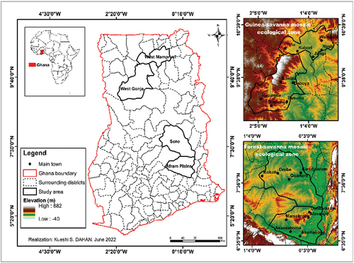
About Forest-Savannah, the districts considered (Sene, Afram Plain), for this research are located between 6° 35ˈ0‘and 8°9ˈ0’ N latitude and 1°40ˈW and 0°31ˈ0” E longitude with an area of 13,880.41 km2. Structured into several sub-zones, the Forest-Savannah zone is located in central Ghana and composed of the Main, Eastern and Central Transitional Zones (MTZ, ETZ and CTZ) with an intermediate climate with two rainy seasons and transitional Forest-Savannah vegetation (Figure 1). The significant commercial tree species include Milicia excelsa (Welw.) C.C.Berg (Odum), Antiaris africana Engl. (kyenkyen or chenchen), and Triplochiton scleroxylon K.Schum. (wawa). The area is also dominated by some native and indigenous species (Nindel, 2017). Local species that cover the area are Celtis mildbraedii Engl. (esa), Entandrophragma angolense (Welw.) Panshin (edinam), Pycnanthus angolensis (Welw.) Warb. (otie), Piptadeniastrum africanum (Hook.f.) Brenan (dahoma), Amphimas pterocarpoides Pierre ex Harms (yaya), Chrysophyllum albidum G.Don (akasaa), and Daniellia ogea (Harms) Rolfe ex Holland (hyedua). The landscape can be described as a mosaic of diverse elements including forest types, human settlements, hydrological systems, and agroecological niches (Ayivor et al., 2015).

Material and data

In this study, sentinel-2B images were used for data collection because of their spatial resolution (10–60 m), fine temporal resolution (five days) and fine spectral resolution of 13 spectral bands particularly well suited for LULC classification (Li & Roy, 2017; Pirotti et al., 2016; Song et al., 2017). These images, which are introduced in the IMPAC toolbox system, are taken from the Copernicus Open Access Hub (https://scihub.copernicus.eu/) (Table 1). Concerning de classification, Landsat images were acquired on the Earth Explorer website (https://earthexplorer.usgs.gov/) with less than 10% cloud cover (Table 2). The use of Landsat images for LULC mapping is justified by their good characteristics. A temporal resolution of 16 days for Landsat 4, 5, 7 and 8; a good spatial resolution (30 m after resampling). Each image set covers an area of 185 km², with an overall spatial resolution of 30 metres. This allowed us to better identify and characterise the different types of LULC on the ground and better make the classification. Image classification, geoprocessing and analysis of the results were done using the following software: Envi 4.7 and 5.3: It has been used for pre-processing and processing of Landsat and Sentinel-2B images; image transformations, contrast enhancement of pre-processed images and classification. ArcGIS Desktop version 10.5: was used for the geoprocessing of LULC data and various cartographic renderings. For the analysis, Excel and Pontius software have been used. For this purpose, the intensity of degradation (Intensity Analysis) and change of LULCs was evaluated through Pontius (PontiusMatrix42). Pontius is an open-source Microsoft Excel programme available at https://www2.clarku.edu/faculty/rpontius/ (Aldwaik et al., 2015; Pontius, 2019b; Pontius & Millones, 2011; Pontius & Santacruz, 2014b).

Table 1. Sentinel images used for automatic classification in IMPACT toolbox.

		Sensor	Tile Number	Acquisition date	Bands combination
Guinea-savannah	2021	Sentinel-2B	T30PXR	18/09/2021	B12, B8, B4
	2021	Sentinel-2B	T30PXS	18/09/2021
	2021	Sentinel-2B	T30PYR	18/09/2021
	2021	Sentinel-2B	T30PYS	18/09/2021
Forest-savannah	2021	Sentinel-2B	T30NYN	01/01/2021
	2021	Sentinel-2B	T30NYP	01/01/2021
	2021	Sentinel-2B	T30NZN	01/01/2021
	2021	Sentinel-2B	T30NZP	01/01/2021
	2021	Sentinel-2B	T30PYQ_	01/01/2021
	2021	Sentinel-2B	T30PZQ_	01/01/2021

Table 2. Landsat images used for the classification.

	Years	Sensors	Path and Row	Acquisition dates	Composite Colors
Guinea-savannah	2001	Landsat 7 ETM+	194_53	27/10/2001	6,4,2
		Landsat 7 ETM+	194_54	27/10/2001
		Landsat 7 ETM+	195_53	03/11/2001
		Landsat 7 ETM+	195_54	03/11/2001
	2011	Landsat 7 ETM+	194_53	26/12/2011	6,4,2
		Landsat 7 ETM+	194_54	26/12/2011
		Landsat 7 ETM+	195_53	17/12/2011
		Landsat 7 ETM+	195_54	17/12/2011
	2021	Landsat 8 OLI TIRS	194_53	13/12/2021	4,5,6
		Landsat 8 OLI TIRS	194_54	29/12/2021
		Landsat 8 OLI TIRS	195_53	20/12/2021
		Landsat 8 OLI TIRS	195_54	20/12/2021
Forest-savannah	2001	Landsat 7 ETM+	193_54	07/12/2001	5,4,2
		Landsat 7 ETM+	193_55	06/02/2001
		Landsat 7 ETM+	194_54	12/01/2001
		Landsat 7 ETM+	194_55	14/12/2001
	2011	Landsat 7 ETM+	193_54	01/01/2011	6,4,2
		Landsat 7 ETM+	193_55	17/01/2011
		Landsat 7 ETM+	194_54	24/01/2011
		Landsat 7 ETM+	194_55	24/01/2011
	2021	Landsat 8 OLI TIRS	193_54	20/01/2021	7,5,4
		Landsat 8 OLI TIRS	193_55	04/01/2021
		Landsat 8 OLI TIRS	194_54	27/01/2021
		Landsat 8 OLI TIRS	194_55	27/01/2021

Methods of image processing and LULC assessment

Preparations for data collection and choice of sites to visit

• Sentinel 2-B image processing

In this part dedicated to the preparation of the field data collection, an automated classification approach was adopted using the IMPACT toolbox to have an idea of the land units based on the visual interpretation approaches of the satellite images and the spectral reactions without forgetting the information obtained through the literature review. This software is downloaded on the Forest Resources and Carbon Emissions (IFORCE) site (http://forobs.jrc.ec.europa.eu/products/software). Thus, the IMPACT toolbox (Image Processing) has been designed to offer a combination of functions for remote sensing, photo interpretation and processing technologies in a portable and stand-alone GIS environment, allowing non-specialist users to easily accomplish all necessary pre-processing steps while giving a fast and user-friendly environment for visual editing and map validation (Simonetti and et al., 2015). The IMPACT toolbox allows for data extraction, layer stacking, radiometric calibration, normalisation, mosaicking, automatic classification and segmentation. The image size and the processing time have concerned three bands (B12, B08, B04) because they retain enough spectral information to successfully use the Index Builder (e.g. NDVI) and Image Segmentation while offering excellent contrast for visual interpretation.

Following this automatic classification, control points were selected and LULC were defined for each study area (Table 3, Figure 2) based on knowledge from the literature review.

Figure 2. LULC of Guinea-savannah (a) and Forest-savannah mosaic (b)zones using IMPACT toolbox.

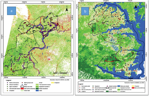
Table 3. Guinea-savannah zone and Forest-savannah mosaic zone control points.

control pints	number
Guinea-savannah zone
Closed woodland	83
Open woodland	93
Tree-savannah mosaic	103
Cropland	149
Built-up bare soil	108
Additional field points	242
Total	778
Forest-savannah mosaic zone
Grassland	14
Mosaic forest-savannah	20
water body and wetland	21
degraded woodland	34
closed woodland	24
Additional field points	160
Total	273

Field data collection

On the field, the pre-selected points have been located using GPS (Global Positioning System). A visual description of their corresponding LULC has been made according to the typology of the vegetation using the categorisation proposed by the FAO (2001) (Table 4). In addition to the previously selected points, further validation points (242 in the Guinea-savannah zone and 160 in the Forest-savannah zone) will be taken in the field using GPS. The focus in the field will be on all types of LULC and more specifically on degraded areas and forests in more or less good condition. Interpretation of the information from the images will allow us to pre-select several areas with good vegetation cover that we will visit. In addition to these areas, other vegetation formations will be visited.

Table 4. Typology of the vegetation categorisation (FAO, 2001).

Canopy density (%)	Canopy class	Probable land use
0–10 %	Very open	Grassland savannahs, bare soil
10–40 %	Open	Open forests, shrubby savannahs, croplands
40–70 %	Moderately dense	Fragmented forests, wooded savannahs
70–100 %	Very dense	Evergreen forest

Adoption of the caption

Several LULC types were described on the field (according to their characteristics), to elaborate the vegetation cover dynamics maps. Then, (6) major LULC units were adopted to achieve the objectives according to each zone, Guinea-savannah (Cropland, water, Degraded woodland, Dense woodland, Tree-savannah mosaic, Bare soil and Built-up) and Forest-savannah (Bare soil and Built-up, Degraded woodland, Dense woodland, Forest-savannah mosaic, Cropland, Water and wetland). These LULC units are thus considered throughout this research.

Image classification and map production

Image pre-processing: radiometric and atmospheric correction

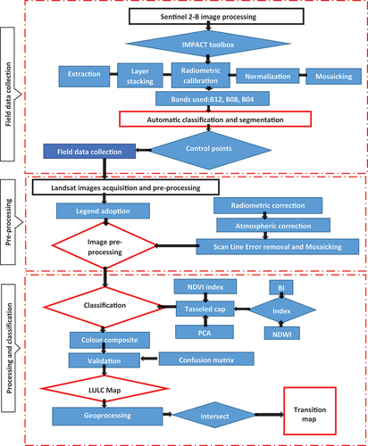
Satellite image pre-processing (Figure 3) is a set of operations that will increase the readability of the images, facilitate their interpretation and have a better extraction of the information (Eckhardt and Moore 1990; Rahman and Dedieu, 1994).

Figure 3. Flow chart of the images’ classification methodological framework.

• Radiometric and atmospheric correction of Landsat images

FLAASH module of the ENVI 5.3 software has been used to make radiometric and atmospheric corrections through Radiometric calibration extension. This tool was used to display the parameter integration table (Radiometric calibration). The following parameters were first entered: calibration type (radiance image); output interleave (BIL); output data type (Float); scale factor (0.10); and Apply FLAASH Settings. Finally, the final operation will be launched (ok) while choosing the place of storage. This correction was important because it improve the readability of the images. This process was followed by the removal of dark masks (Scan Line Error) on some images (Landsat_gapfil) and mosaicking (Mosaicking => Seamless mosaic) as the study areas cover several scenes.

• Calculation of Normalised Vegetation Index (NDVI), Tasseled Cap transformation, and principal component analysis (PCA) analysis

Normalised vegetation index (NDVI), which allowed vegetation and bare soil to be highlighted has been calculated. The NDVI is chosen because it is a potential biophysical indicator of climate that reflects the photosynthetic activity of the vegetation cover at the time of measurement (Rouse et al., 1974). Also, NDVI is the first and most known vegetation index to explore and detect vegetated areas and plant canopies (Rousse et al., 1974). It is calculated according to the following formula:

(1) $NDVI=\left(\left(NIR-R\right)\right)/\left(\left(NIR+R\right)\right)$(1)

Where: NIR is the reflectance of the vegetation in the near-infrared and R is the reflectance in the red. Thus, the NDVI is calculated from the TM, ETM+ and OLI TIR bands, Respectively. Its value lies between −1 and 1. The closer to 1, the higher the normalised vegetation index.

• The Brightness Index has been applied after Tasseled Cap Transformation (Crist and Cicone, 1984). It is an index that is sensitive to the brightness of soils and allows for better discrimination of bare soils from other LULC typologies.

(2) $BI=R^2+NI{R}^2\hspace{0.17em}{)}^{\frac{1}{2}}$(2)

• The Wetness Index after Tasseled Cap Transformation (Crist and Cicone, 1984) or Wetness Index (WI) was also applied. For better classification, the NDWI (Normalized Difference Water Index) maximises the reflectance of water using the green band and minimises the reflectance of water masses using the near-infrared, on Landsat images. The NDWI, based on the combination of the green band with the NIR or SWIR, is a good indicator of the liquid water content of vegetation and is at the same timeless sensitivity to the effects of atmospheric scattering than the NDVI (Gao,1996). Its usefulness for drought monitoring and early warning has been demonstrated in different studies (Gu et al., 2007; Ceccato et al., 2002).

(3) $NDWI=\left(Green-SWIR\right)/\left(Green+SWIR\right)$(3)

These different indices (NDVI, NDWI, BI and Tasseled Cap transformation) were applied to the images to better detect the LULC

typologies

• Principal Component Analysis (PCA)

PCA is an image processing technique that concentrates the main information in the first three (3) bands. It converts the correlated multispectral bands into a new set of uncorrelated components. The resulting PCA bands have non-redundant information and provide enhanced accuracy in features-based image identification and classification as compared to other techniques (N’da et al., 2008). This satellite image classification technique has been used by several other authors (Doshvarpassand & Wang, 2021; Rwanga & Ndambuki, 2017; Li et al., 2015) and has allowed us to better identify the bands with the most information so that our classification reflects the reality of the field.

Classification: composite colours

Following the normalised vegetation index, Tasseled Cap transformation, and principal component analysis (PCA), the colour composition has been applied to have more precise spectral discrimination of the different types of LULC. This treatment was based on the knowledge of the spectral behaviour of the different types of LULC in the various wavelengths and their exploitation in an additive synthesis of primary colours Red-Green-Blue and secondary colours (Cyan-Magenta-Yellow) (Dahan et al., 2021). In this study, supervised classification has been used. It is, therefore, part of a classic supervised classification pathway. This classification is used given the fieldwork that is planned in this study. It consists of visually identifying a certain number of natural or artificial elements or objects that can be punctual, linear or surface on the image. This classification was carried out in ENVI 4.7.

The units: Cropland, water, Degraded woodland, Dense woodland, Tree-savannah mosaic, Bare soil and Built-up for the Guinea-savannah zone whereas for the Forest-savannah zone, Bare soil and Built-up, Degraded woodland, Dense woodland, Forest-savannah mosaic, Cropland, Water and wetland have been defined for the legend. This has led to the selection of the training plots. Thus, these classes were defined and followed by the assignment of colours. The Maximum Likelihood algorithm has been chosen for the classification because it allows us to better compare the results obtained with the reality of the field. It allows us to classify the unknown pixels by calculating for each class the probability that the pixel falls into the corresponding class. However, if this probability does not reach the expected threshold, the pixel is classified as unknown.

Evaluation and validation of the supervised classification

The validation of the classification was done in two steps. The first step was a visual thematic analysis comparing the basic colour compositions and the resulting maps. For this purpose, a visual comparative analysis of the basic colour composition and the produced LULC map was carried out. When there is conformity between the two data then the thematic analysis will be validated. The second step was an analysis of the confusion matrices to evaluate the performance level of the processing, but also of the LULC classes through the overall accuracy and the Kappa coefficient. According to Skupinski et al. (2009), the Kappa index characterises the ratio between the well-classified pixels and the total number of pixels surveyed. Once the classification has been validated by the various performance tests above, a 3 × 3 median filter is applied to reduce intra-class heterogeneity by eliminating isolated pixels. The confusion matrix is presented as follows: the lines represent the assignment of pixels to each theme after classification, the columns show the actual distribution of pixels in each theme, and the diagonal represents the percentages of well-ranked pixels. The final step for image processing was the vectorisation. This consists of converting the classified image from raster format to vector format (FVF) and then converting it into a shapefile format (SHP) which can be handled in a Geographic Information System (GIS). It was done through ENVI 4.7 software through the classification tool (Post classification > Classification to vector).

Geoprocessing and change detection map creation

After having produced the different LULC maps of the selected years, the geoprocessing consisted of merging the maps two by two (2001–2011; 2011–2021 and 2001–2021) through the ‘Intersect’ algorithm (ArcGIS 10.5) to change detection maps using the following categories: Gain areas, Loss areas and Stable areas based on the conversion of vegetated areas into of non-vegetated areas and vice versa. The changes are obtained in the attribute table by using the coding technique of converting the occupation unit from year A to year B (Table 5) through the Field calculator in the table of attributes by selecting the change path already created. This process allowed us to produce three change detection maps per zone:

Table 5. Use of the Intersect module in the geoprocessing tool to create the change detection map.

Year A	Year B	Conversion code	Example of change	Categories
Degraded forest	Dense forest	[A] + ‘-’ + [B]	Degraded forest to Dense forest	Gain area
Dense forest	Forest-savannah mosaic	[A] + ‘-’ + [B]	Degraded forest to forest-savannah mosaic	Loss area
Built-up	Built-up	[A] + ‘-’ + [B]	Built-up to Built-up	Stable area

Evaluation of changes between LULC and intensities analysis from 1991 to 2021

Intensity Analysis is a mathematical framework to express differences within a set of categories that exist at multiple time points (Quan et al., 2019). At this step, a post-classification comparison method, which is a common approach for evaluating differences in LULC maps derived from satellite images acquired on different dates has been used (Mundia & Aniya, 2005; Vasconcelos et al., 2002; Yang & P, 2002; Yuan et al., 2005). This procedure involves data preprocessing, image classification, and change detection. This allowed us to have the transition matrixes (1991–2011, 2011–2021 and 1991–2021). The LULC transition matrix aims to quantify a system state and state transition by comparing maps of different periods, as it provides information on ‘from-to’ class changes (Teferi et al., 2013; Zhang et al., 2017).

Details on the change of LULC units can be seen in the transition matrix, however, further investigation is needed to link the models to processes (Zaehringer et al., 2015). Thus, intensity analysis is timely as it is a set of related approaches that facilitate a more in-depth analysis. Intensity analysis is an accounting framework for describing the behaviour of a categorical variable across time intervals and measuring the degree of non-uniformity of changes at different levels of detail (Aldwaik & Pontius, 2012; Enaruvbe & Pontius, 2015). The interval level highlights the overall variation during one interval to the overall variation during one or more other intervals. The category level describes the variation in gross loss intensity and gross gain intensity between categories (LULC) in each time interval. The transition level describes the variation in the intensity with which the gain of a particular category moves from one category to another in each time interval (Aldwaik & Pontius, 2012, 2013). Our analysis uses five equations whose notation is shown in Table 1 (Aldwaik & Pontius, 2012). Many studies have used intensity analysis to evaluate LULC degradation and changes (Alo & Pontius, 2008; Asenso Barnieh et al., 2022; Ekumah et al., 2020; Enaruvbe & Pontius, 2015; Manandhar et al., 2009; Zhou et al., 2014; Quan et al., 2020). In our analysis, we will focus on the change in categories and their intensity of change to get an idea of which tenure units are more vulnerable.

Analysis of the sizes of the change components; exchange and shift components (allocation change) and quantity component (net change)

Based on the transition matrices obtained (Tables 6) according to each interval (1991–2011; 2011–2021 and 1991–2021), the overall difference (the total change) in each time interval for each unit category was categorised into net change, exchange and displacement (Pontius, 2019a; Pontius & Santacruz, 2014a). Total change, i.e. the sum of gross losses and gross gains in the study areas, was estimated by applying equation (4) following the applied mathematical notations (Tables 6 and 7). For each category, the gross loss was calculated by summing the off-diagonal entries of the corresponding row. Similarly, the gross gain for each category was estimated by adding the off-diagonal entries in each column. Equation (6) adds up all the entries in the matrix for each category and subtracts the entry from the diagonals to obtain the gross change for each category (Pontius, 2019a; Quan et al., 2019). The quantitative component (net change) for an arbitrary category j was estimated by subtracting the gross loss, i.e. the row totals, from the gross gain, i.e. the column totals. This was done by applying equation (7). The net change masks how a given transition occurs since it is likely that category i moves to category j at some locations while category j moves to category i at other locations in a given area (spatial reallocation of LULCs at a given time). The simultaneous spatial reallocation between a pair of LULC categories can be described as an exchange (Pontius, 2019a; Quan et al., 2019). The size of the exchange component was estimated by applying equation (3)(3) $NDWI=\left(Green-SWIR\right)/\left(Green+SWIR\right)$(3) , which gives the exchange as two multiplied by the minimum of C_ij and C_ji since the exchange occurs between two pairs of categories, i.e. i and j. Here, the minimum function was applied because the smallest input between C_ij and C_ji limited the estimation of the exchange. Therefore, it may happen that a fraction of category i at the initial time moves to category j at the final time, while at the same time category i gains a third category k. This component of change is referred to as a lag (Pontius, 2019b; Pontius & Santacruz, 2014b). Equation (8) was used to calculate the component of change for an arbitrary category j (Table 6). The overall difference (total size of change) was calculated with Eq. (9) in Table 7. The result of this estimation is equivalent to the sum of the three components: net change (quantity change), exchange and change (allocation change). Thus, the estimated overall sizes of these components were calculated for the whole area and were of the same magnitude (equations 10 to 11 respectively). The numerators of equations (8) to (11) were all divided by two as each of the differences in the numerator was counted twice in the summations.

Table 6. Mathematical notations in the change components equations (Pontius Jr. (2019).).

Symbols	Descriptions
J	Number of categories
i	Index for a category of a row
j	Index for a category of a column
Cij	Size of spatial extent that is in row and column j of the contingency table
Cji	Size of spatial extent that is in row and column i of the contingency table
dj	Difference for category j
qj	Quantity component for category j
ej	Exchange component for category j for an interval
Sj	Shift component for category j for an interval
D	Overall difference for an interval
Q	Overall quantity component for an interval
E	Overall exchange component for an interval
S	Overall shift component for an interval
${\hspace{0.17em}}_{q_j}^{\hat{A}\underset{{ }_{.}}{\prime }}$	Quantity Intensity of category j
${\hspace{0.17em}}_{e_j}^{\hat{A}\underset{{ }_{.}}{\prime }}$	Exchange Intensity of category j
${\hspace{0.17em}}_{s_j}^{\hat{A}\underset{{ }_{.}}{\prime }}$	Shift Intensity of category j
${\hspace{0.17em}}_Q^{\hat{A}\underset{{ }_{.}}{\prime }}$	Quantity Intensity Overall
${\hspace{0.17em}}_E^{\hat{A}\underset{{ }_{.}}{\prime }}$	Exchange Intensity Overall
${\hspace{0.17em}}_S^{\hat{A}\underset{{ }_{.}}{\prime }}$	Shift Intensity Overall

Table 7. Estimations of the change components defined equations (Pontius Jr., 2019; Pontius Jr. And Santacruz, 2014).

$d_j$ = $\left[\hspace{0.17em}\sum _{i=1}^n\hspace{0.17em}\left(C_{ji}+C_{ji}\right)\hspace{0.17em}\right]-\hspace{0.17em}$2 × $C_{ji}$	Equation (4)
$q_{tj}$= $\left|\hspace{0.17em}\sum _{i=1}^n\hspace{0.17em}\left(Cij+Cji\right)\right|$	Equation (5)
$e_j$ = 2 ×$\left\{\hspace{0.17em}\left[\hspace{0.17em}\sum _{i=1}^{n}MINIMUM\left(C_{ji}+C_{ji}\right)\hspace{0.17em}\right]-C_{tji}\right\}$	Equation (6)
$s_j$= $d_j$– $q_j$ – $e_j$	Equation (7)
D = $\frac{\hspace{0.17em}{\sum }_{j=1}^{J}dj}{2}=Q+E+S$	Equation (8)
Q = $\frac{\hspace{0.17em}{\sum }_{j=1}^{J}qj}{2}$	Equation (9)
E = $\frac{\hspace{0.17em}{\sum }_{j=1}^{J}ej}{2}$	Equation (10)
S = $\frac{\hspace{0.17em}{\sum }_{j=1}^{J}Sj}{2}=D-Q-E$	Equation (11)
${\hspace{0.17em}}_{q_j}^{\hat{A}\underset{{ }_{.}}{\prime }}$= $\frac{100\%qj}{dJ}$	Equation (12)
${\hspace{0.17em}}_{e_j}^{\hat{A}\underset{{ }_{.}}{\prime }}$ = $\frac{100\%ej}{dJ}$	Equation (13)
${\hspace{0.17em}}_{s_j}^{\hat{A}\underset{{ }_{.}}{\prime }}$ = $\frac{100\%sj}{dJ}$	Equation (14)
${\hspace{0.17em}}_Q^{\hat{A}\underset{{ }_{.}}{\prime }}=\frac{100\mathrm{\%}Q}{D}=\sum _{j=1}^J\left[{\hspace{0.17em}}_{qj}^{\hat{A}\underset{{ }_{.}}{\prime }}(dj/2D)\right]$	Equation (15)
${\hspace{0.17em}}_E^{\hat{A}\underset{{ }_{.}}{\prime }}=\frac{100\mathrm{\%}Q}{D}=\sum _{j=1}^J\left[{\hspace{0.17em}}_{ej}^{\hat{A}\underset{{ }_{.}}{\prime }}(dj/2D)\right]$	Equation (16)
${\hspace{0.17em}}_S^{\hat{A}\underset{{ }_{.}}{\prime }}=\frac{100\mathrm{\%}Q}{D}=\sum _{j=1}^J\left[{\hspace{0.17em}}_{sj}^{\hat{A}\underset{{ }_{.}}{\prime }}(dj/2D)\right]$	Equation (17)

Analysis of the intensity of the components of change

The intensity of each component by category was estimated by equation (12–14). It is given by the size of the category component divided by the size of the category difference (change) in per cent. The intensities estimated from equation (12–14) range from 0% to 100%, i.e. for a given category ($\hat{A}\underset{{ }_{.}}{\prime }/q_j$, $\hat{A}\underset{{ }_{.}}{\prime }/e_j$ and $\hat{A}\underset{{ }_{.}}{\prime }/s_j$) sum to 100%. The overall intensity of each component was calculated by dividing the overall component sizes by the overall difference size expressed as a percentage (see equations (15)- (17)). Here, the total weighted average of the components for each category is equal to 1 in fractional terms or 100% in percentage terms. This implies that the intensities estimated from equations (15) - (17) range from 0% to 100 and thus the sum of $\hat{A}\underset{{ }_{.}}{\prime }/Q$, $\hat{A}\underset{{ }_{.}}{\prime }/E$ and, $\hat{A}\underset{{ }_{.}}{\prime }/S$ amounts to 100% in terms of percentage or 1 in terms of fraction, irrespective of the sizes of the categories and the corresponding differences. Any deviation from the overall component for a given category indicates that the estimated component is active, i.e. if the example $\hat{A}\underset{{ }_{.}}{\prime }/q_j$ > $\hat{A}\underset{{ }_{.}}{\prime }/Q$, this implies that the quantitative component for category j is intensive and vice versa. This allowed for comparisons between categories as well as comparisons of the respective components of different categories with the corresponding global component (Pontius, 2019a).

Results

The results of the classification revealed six land-use units within each ecological zone (Guinea-savannah zone and Forest-savannah mosaic zone). These units were the subject of our classification as they represent the majority of LULCs present in the field. Thus, the units: cropland, water, Degraded woodland, Dense woodland, Tree-savannah mosaic, Bare soil and Built-up (Guinea-savannah zone) and Bare soil and Built-up, Degraded woodland, Dense woodland, Forest-savannah mosaic, Cropland (Forest-savannah mosaic zone) were retained, evaluated and analysed. From this classification, the overall accuracy and Kappa coefficient varied between 88–96% and 88–93% respectively in the two ecological zones (Table 8). These values allowed us to validate the classification for further analysis as they are within the generally accepted validation range for satellite image classification (Lillesand et al., 2014; Ukrainski, 2016).

Table 8. Overall accuracy and Kappa coefficient obtained for each image per region.

	Years	Overall Accuracy (%)	Kappa Coefficient (%)
Guinea-savannah zone	2001	93%	91%
	2011	88%	85%
	2021	91%	89%
Forest-savannah mosaic zone	2001	91%	88%
	2011	93%	89%
	2021	96%	93%

Vegetation cover dynamics in the Guinea-Savannah zone

The overall trend after image classification (Figure 5), the LULC units between the years 2001 and 2021 through 2011 (Figure 4) show an increase in the area of Degraded woodland and Tree-savannah in favour of the other LULC units. There is also a regression of cultivated areas and a considerable increase of Bare soil and Built-up with a slight increase of Dense woodland. These units occupy the following areas according to each year: cropland (23508.51 Km² or 65.42%), water (38.1 Km2 or 0.11%), Degraded woodland (1540.64 Km² or 4.29%), Dense woodland (2935.98 Km² or 8.17%), Tree-savannah mosaic (7026.7 Km2 or 19.55%), Bare soil and Built-up (886.66 Km² or 2.47%) in 2001, cropland (41.05 Km2 or 0.11%), water (1587.85 Km² or 4.42%), Degraded woodland (1587.85 Km² or 4.42%), Dense woodland (3562.31 Km² or 9.91%), Tree-savannah mosaic (6162.14 Km² or 17.15%), Bare soil and Built-up (23928.32 Km² or 66.58%) in 2011 while in 2021, the surfaces are evaluated at 1050.38 Km² or 2.92% for cropland, 65.72 Km² or 0.18% for water, 3434.29 Km² or 9.56% for Degraded woodland, 4309.19 Km² or 11.99% for Dense woodland, 2110.09 Km² or 5.87% for Tree-savannah mosaic and 24,966.9 Km² or 69.47% for Bare soil and Built-up (Table 9). This result shows the overall importance of anthropogenic pressure in the area, given the considerable increase in the area of inhabited zones and night soil.

Figure 4. Proportion of LULCs by year in Guinea-savannah zone (2001–2021).

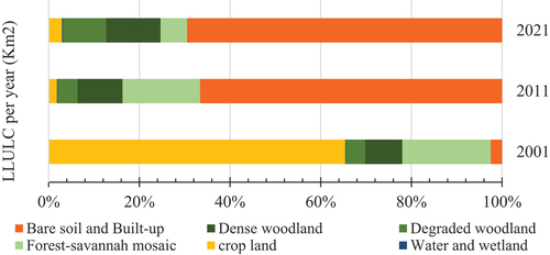
Figure 5. LULC maps of the districts in the Guinea-savannah zone.

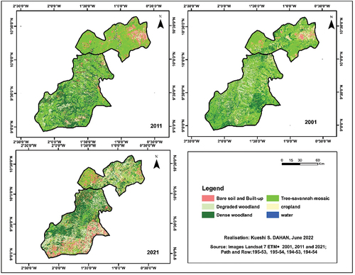
Table 9. Change in LULCs from 2001 to 2021 in Guinea-savannah zone.

		2001		2011		2021
		Km^2	%	Km^2	%	Km^2	%
Guinea-savannah zone LULCs surface areas	cropland	23508.51	65.42	654.91	1.82	1050.38	2.92
	water	38.1	0.11	41.05	0.11	65.72	0.18
	Degraded woodland	1540.64	4.29	1587.85	4.42	3434.29	9.56
	Dense woodland	2935.98	8.17	3562.31	9.91	4309.19	11.99
	Tree-savannah mosaic	7026.7	19.55	6162.14	17.15	2110.09	5.87
	Bare soil and Built-up	886.66	2.47	23928.32	66.58	24966.9	69.47
	Total	35936.59	100	35936.59	100	35936.59	100

Global changes from 2001 to 2021

The Guinea-Savannah zone across the districts considered for 2001, 2011 and 2021 LULC maps showed the existence of changes in vegetation cover in terms of degradation of vegetation zones (Table 10). These changes led to areas of vegetation gain, loss and stability (Figures 6 and 7). The categories of gain, loss and stability of vegetation were assessed about the decrease or increase of a vegetation entity. The others are thus classified as stable areas. The result is that the whole study period showed more loss than gain as well as stability. The gains and losses are the result of the conversion of certain LULC units into others such as Dense woodland and/or Tree-savannah mosaic into Cropland and/or Bare soil and built-up vice versa. The changes although recorded loss over the whole period (6391.59 Km² or an average of 456.54 Km²), the losses were more observed during the last decade (2011–2021) with a total area of 6442.33 Km² or 460.17 Km2 of vegetation cover lost. The gains and stable areas are more observed during the first decade (2001–201) respectively 4037.34 Km² or an average of 269.16 Km² and 6058.01 Km2 or 403.87 Km².

Figure 6. Categories of changes observed in the Guinea-savannah zone (2001–2021).

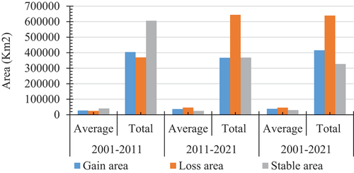
Figure 7. Change detection maps of LULC units from 2001–2021 in the Guinean-savannah zone.

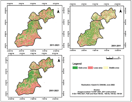
Table 10. Statistics on gains, losses and stable areas in Guinea-savannah zone.

	2001–2011		2011–2021		2001–2021
Area (Km^2)	Average	Total	Average	Total	Average	Total
Gain area	269.166	4037.34	366.94	3669.42	377.62	4153.78
Loss area	246.28	3694.18	460.17	6442.33	456.54	6391.59
Stable area	403.87	6058.01	245.79	3686.88	297.45	3271.96

Analysis of the intensities of the change components Guinea-savannah zone

Exchange and shift components or Allocation Change

Overall, the exchange component was the second largest component at the level of the spatial aggregation considered (Guinea-savannah zone) for the entire period 2001–2021 (Figures 8 and Table 11). Within this spatial aggregation, overall landscape exchange was highest for Dense woodland, followed by Cropland and then the other LULCs for the period 2001–2011 (Figures 8 and Table 11). For the same period, the exchange was lower for all categories compared to the whole period (2001–2021). The other LULC types, Bare soil and built-up and water respectively recorded the highest exchange intensity (Figures 8 and Table 11). It should be noted that the intensity is more observed during the period 2011–2021. In the period 2001–2011 and over the whole period 2001–2021, the loss exchange was higher for the LULC types, Degraded woodland, while the others achieved a low loss. For the period 2011–2021, there is a loss in the vegetation units Degraded woodland and Dense woodland: Degraded woodland and Dense woodland.

Figure 8. Overall difference change (quantity (net change), exchange and shift) sizes (a_1s-a_3s), simultaneous gains and losses (c_1s-c_3s) during 2001–2011; 2011–2021; 2001–2021 and intensities of losses and gains (b_1s-b_3s; d_1s-d_3s) during the same period in Guinea-savannah zone. The categories are labelled ‘loss’ if the LULC unit losses between given intervals outweigh the LULC unit gains and vice versa (see additional materials).

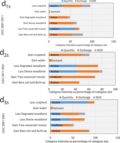
Table 11. Change intensities for quantity change, exchange and shift components for each land use land cover (LULC) category at different spatiotemporal scales in Guinea-savannah zone during 2001–2011, 2011–2021 and 2001–2021.2021.The entries labelled ‘extent/overall’ represent the uniform intensities.

	Quantity Change (%)	Exchange (%)	Shift (%)	Quantity Label
Category Guinea-savannah zone 2001–2011
cropland	19	55	26	Loss
water	84	16	0	Gain
Degraded woodland	39	53	7	Gain
Dense woodland	36	57	7	Gain
Tree-savannah mosaic	72	21	7	Loss
Bare soil and Built-up	37	43	20	Gain
Extent/overall	50	39	11	Extent
Category Guinea-savannah zone 2011–2021
cropland	48	43	9	Gain
water	75	23	2	Gain
Degraded woodland	39	61	0	Loss
Dense woodland	35	56	9	Loss
Tree-savannah mosaic	42	57	1	Gain
Bare soil and Built-up	56	44	0	Gain
Extent/overall	43	52	4	Extent
Category Guinea-savannah zone 2001–2021
cropland	75	24	1	Loss
water	73	22	5	Gain
Degraded woodland	17	61	22	Loss
Dense woodland	41	55	4	Loss
Tree-savannah mosaic	37	31	32	Gain
Bare soil and Built-up	90	10	0	Gain
Extent/overall	45	43	13	Extent

In contrast, Degraded woodland, Dense woodland and Tree-savannah mosaic recorded the largest difference in trade over the periods considered, namely 2001–2011, 2001–2021 and 2001–2021 (Figures 8 and Table 11).

All categories of LULC have experienced active losses as well as gains, except Water (dormant) concerning the intensity of uniform change (Tree-savannah mosaic) (Figures 8 and Table 11). During the period 2001–2011 and 2001–2021, Cropland, and Tree-savannah mosaic, respectively suffered the losses in the study area. However, for the period 2011–2021, losses were recorded in Degraded woodland and Dense woodland, the others experienced gains.

In the period 2011–2021, the exchange of losses was highest for Degraded woodland and Dense woodland than the other periods (2001–2021 and 2001–2021). The intensity of gross losses was active for the vegetation zones (Degraded woodland, Dense woodland) as well as Bare soil and Built-up, and Cropland. However, Water was losing dormant, while the Tree forest-savannah mosaic was uniform (Figures 8 and Table 4).

About transfer, the majority of occupancy units have transferred proportions over the whole period considered. The transfer is more observed in the period 2001–2011. LULC units such as Water, Tree-savannah mosaic (2001–2011 and 2011–2021), Bare soil and Built-up (2011–2021 and 2001–2021) and Cropland (2001–2021) have transferred the most portions of their area.

The difference in lag was observed for the majority of LULC units over all periods considered except for the units of Water in the period 2001–2011, Degraded woodland (2011–2021) and Bare soil and Built-up (2011–2021 and 2001–2021) (Figures 8 and Table 11).

Quantity component (Net Change)

In terms of quantity change (net change), the period between 2001 and 2011 had the highest net change, i.e. the difference in the quantity component over the whole area at the spatial aggregation level (Figures 8 and Table 11). The difference in quantity was highest for Bare soil and built-up over this period, for Water over the period 2011–2021 and for Bare soil and Built-up when considering the whole period (2001–2021). In all the periods considered, the changes in quantity are not made uniformly but it follows that the changes have been more marked in the transition map, in other words, the vegetation dynamics have been carried out during the period 200–2021 through the quantitative changes of the LULCs.

The amount of loss was highest for Dense woodland over the whole period (2001–2021) followed by Degraded woodland. However, gains in quantity were observed in Tree-savannah mosaic, Cropland and Water during the period 2001–2021, while Bare soil and Built-up had the highest differences in the quantity of gain at all intervals and different levels of spatial aggregation (Figures 8 and Table 11). But in the last decade, Water has experienced more change in terms of quantity difference followed by Bare soil and Built-up and Degraded woodland.

Detailed intensities of the change components at different spatiotemporal scales

To assess the intensity of change in the LULCs of the study area, Table 4 presents the total normalised change (net/quantitative change, change and shift) for each category in terms of percentages on the 0–100% scale obtained. Overall, the quantity change was the largest proportion of the three components for this period. LULC units such as Water, Cropland and Bare soil and Built-up achieved the highest level of quantity change. The transfer was highest for Cropland, Bare soil and Built-up, Degraded woodland and Tree-savannah mosaic.

The intensity of losses and gains were active for all categories of LULCs, except for Water, which was dormant in terms of gains and losses (Figure 8 and Table 4). The observed change across the area was different between 2001 and 2021 for the three main components (net change/quantity, exchange and displacement). During this period, the quantity change (net change) was the highest component in the whole area (Guinea-Savannah). The quantity component was highest for the settlement. The net/quantity change was qualified as a gain for Water, Tree-savannah mosaic, Bare soil and Built-up. Loss intensities are observed in Cropland, Degraded woodland and Dense woodland. These loss intensities are generally active for the vegetation units (Degraded woodland and Dense woodland). The gain intensities for Water and Bare soil and Built-up are active.

The overall patterns of LULC transitions observed over the whole period (2011–2021) at the ecoregion scale were almost the same as those observed over the period 2001–2021 when considering the exchanges observed in terms of loss in Degraded woodland and Dense woodland.

Overall, it is observed during the period 2001–2011 that the amounts changed in terms of proportion are more considerable, but during the period 2011–2021, the exchanges in proportion between LULCs have taken over. Thus, during 2001–2011, the Tree-savannah mosaic lost more area, while gains are observed at the Water unit. During 2011–2021, the loss intensity is higher in Degraded woodland and Dense woodland and the gain intensity was more observed in Water and Bare soil and Built-up while the whole period shows that the degradation intensity of LULCs is more felt in Degraded woodland, Dense woodland and Cropland. The highest intensity in terms of gain is observed in Bre oil and Built-up (Figure 8 and Table 4).

Vegetation cover dynamics in the Forest-savannah mosaic zone

Concerning the overall trend in the image classification of the Forest-Savannah area (Figure 10), the LULC units from 2001 to 2021 (Figure 9) show an increase in the areas of Degraded woodland, Cropland, Bare soil and Built-up and a decrease in the other LULC units. These land-use units recorded the following areas: Bare soil and Built-up (571.13 Km² or 2.41%), Dense woodland (1378.45 Km² or 5.81%), Degraded woodland (2921.93 Km² or 12.32%), Forest-savannah mosaic (5442.81 Km² or 22.95%), Cropland (461.07 Km² or 19.55%), Water and wetland (12941.2 Km2 or 54.57%) in 2001, Bare soil and Built-up (577.19 Km² or 2.43%), Dense woodland (2497.76 Km² or 10.53%), Degraded woodland (2349.91 Km² or 9.91%), Forest-savannah mosaic (2802.38 Km² or 11.86%), Cropland (3125.46 Km² or 13.18%), Water and wetland (12390.9 Km² or 52.25%) in 2011 while in 2021, the areas are estimated at 2792.6 Km² or 11.77% for Bare soil and Built-up, 748.98 Km² or 3.16% for Dense woodland, 3889.23 Km² or 16.40% for Degraded woodland, 3161.38 Km² or 13.33% for Forest-savannah mosaic and 766.77 Km² or 3.23% for Cropland, 12184 Km² or 51.37% for Water and wetland (Table 12). This is a result of the degradation of vegetated areas at the expense of anthropized areas in the Forest-savannah mosaic ecological zone.

Figure 9. Proportion of LULCs per year in the Forest-savannah mosaic zone (2001–2021).

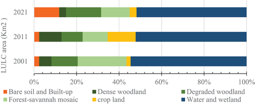
Figure 10. LULC maps of districts in the Forest-savannah mosaic zone (2001–2021).

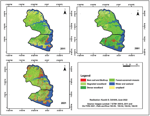
Table 12. Change in LULCs from 2001 to 2021 in Guinea-savannah zone.

		2001		2011		2021
		km^2	%	km^2	%	km^2	%
Forest-savannah zone LULCs surfaces area	Bare soil and Built-up	571.13	2.41	577.19	2.43	2792.6	11.77
	Dense woodland	1378.45	5.81	2497.76	10.53	748.98	3.16
	Degraded woodland	2921.93	12.32	2349.91	9.91	3889.23	16.40
	Forest-savannah mosaic	5442.81	22.95	2802.38	11.86	3161.38	13.33
	cropland	461.07	1.94	3125.46	13.18	766.77	3.23
	Water and wetland	12941.2	54.57	12390.9	52.25	12184	51.37
	Total	23716.54	100	23716.54	100	23716.54	100

Change from 2001 to 2021 in Forest-savannah mosaic zone

The districts considered in the Forest-savannah mosaic zone experienced during 2001–2021 also some changes in the vegetation cover in terms of degradation of vegetation zones (Table 13). The observed changes are also gain, loss and stability of vegetation (Figures 11 and 12). The categories gain, loss and stability of vegetation were evaluated with the decrease or increase of vegetation areas. Stable areas are those that have not experienced any dynamics. The result is that the whole study period has seen more loss than gain as well as stability. The gains and losses are the result of the conversion of some LULC units into others such as Dense woodland and/or Forest-savannah mosaic into Cropland and/or Bare soil and built-up vice versa. Although the transition time recorded a loss of 7616.94 km² over the whole period (2001–2021), i.e. an average of 9037.0 km², the loss of vegetation cover (5089 km² or 391.46 km²) was less observed during the last decade (2011–2021) compared to the first decade (2011–2021) (5992.96 km² or an average of 461 km2). Gains are more observed during the first decade 2001–2011 (2131.38 km² or an average of 193.76 km²) while stabilities are observed in the last decade (6574.65 km² or 505.74 km²).

Figure 11. Categories of changes observed in the Guinea-savannah zone (2001–2021).

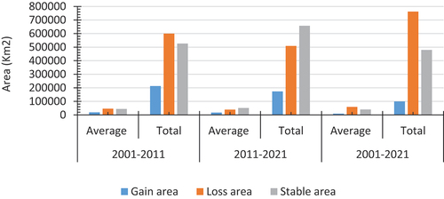
Figure 12. Change detection maps of LULC units from 2001–2021 in the Forest-savannah mosaic zone.

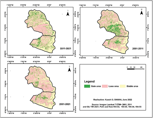
Table 13. Areas of gains, losses and stable areas in Forest-savannah mosaic zone.

	2001–2011		2011–2021		2001–2021
Area (Km^2)	Average	Total	Average	Total	Average	Total
Gain area	193.76	2131.38	173.14	1731.39	90.37	994.07
Loss area	461	5992.96	391.46	5089	585.92	7616.94
Stable area	438.28	5259.33	505.74	6574.65	399.12	4789.30

Analysis of the intensities of the change components in the Forest-savannah zone

Exchange and shift components or Allocation Change

Overall, the exchange component occupies the largest component at the level of the spatial aggregation considered (Guinea-savannah zone) over the period 2001–2021 (Figures 13 and Table 14). Within this spatial aggregation, landscape exchange is highest for the Forest-savannah mosaic, followed by Dense woodland and then the other LULCs for the period 2001–2011. For the same period, the exchange was highest for all categories compared to the period 2001–2021. LULC types such as Bare soil and built-up and water and wetland respectively recorded the highest exchange intensity (Figures 13 and Table 14). The intensity is less observed during the period 2011–2021 overall. During the period 2001–2011 and the whole period 2001–2021 (see Figures 13 and Table 14), the exchange of losses was highest for, Forest-savannah mosaic followed by Bare soil and Built-up, while the others achieved a low loss so dominated by gain. For the period 2011–2021, there was a loss in vegetation units such as Cropland, Water and wetland and Dense woodland.

Figure 13. Overall difference change (quantity (net change), exchange and shift) sizes (a_1f-a_3f) simultaneous gains and losses (c_1s-c_3s) during 2001–2011; 2011–2021; 2001–2021 and intensities of losses and gains (b_1f-b_3f; d_1f-d_3f) during the same period in Forest-savannah mosaic zone. The categories are labelled ‘loss’ if the LULC unit losses between given intervals outweigh the LULC unit gains and vice versa (see additional materials).

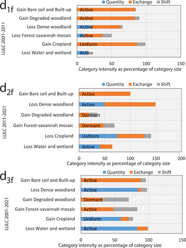
Table 14. Change intensities for quantity change, exchange and shift components for each land use land cover (LULC) category at different spatiotemporal scales in Forest-savannah mosaic zone during 2001–2011, 2011–2021 and 2001–2021.2021.The entries labelled ‘extent/overall’ represent the uniform intensities.

	Quantity Change (%)	Exchange (%)	Shift (%)	Quantity Label
Category Forest-savannah mosaic zone 2001–2011
Bare soil and Built-up	84	16	0	Gain
Degraded woodland	73	25	2	Gain
Dense woodland	19	76	6	Loss
Forest-savannah mosaic	12	59	29	Loss
Cropland	80	18	3	Gain
Water and wetland	87	12	2	Loss
Extent/overall	31	54	15	Extent
Category Forest-savannah mosaic zone 2011–2021
Bare soil and Built-up	80	20	0	Gain
Dense woodland	41	32	27	Loss
Degraded woodland	82	13	6	Gain
Forest-savannah mosaic	83	14	3	Gain
Cropland	61	39	0	Loss
Water and wetland	70	8	22	Loss
Extent/overall	65	25	10	Extent
Category Forest savannah mosaic zone 2001–2021
Bare soil and Built-up	72	26	2	Gain
Dense woodland	76	8	16	Loss
Degraded woodland	80	9	11	Gain
Forest-savannah mosaic	67	19	14	Gain
Cropland	94	6	0	Gain
Water and wetland	79	21	0	Loss
Extent/overall	77	14	9	Extent

All LULC categories have experienced active losses as well as gains, however, units such as Degraded woodland and Forest-savannah are dormant over the period 2011–2021 and 2001–2021 relative to the intensity of uniform change (Cropland) (Figures 13 and Table 4). Over the period 2001–2011. 2011–2021 and 2001–2021, Dense woodland, Forest-savannah mosaic, Dense woodland, Cropland, Water and wetland, respectively suffered the losses in the study area. However, for the period 2011–2021, gains were recorded in Degraded woodlands, Bare soil and Built-up and Forest-savannah mosaic.

Over the period 2011–2021, exchange in terms of losses was highest for Cropland while Dense woodland experienced more exchange over periods (2001–2011). Gross loss intensity was active for Dense woodland as well as Bare soil and Built-up, Forest-savannah, Water and wetland. However, Degraded woodland was a dormant loser, while Cropland was uniform (Figures 13 and Table 14).

About transfer, the majority of occupancy units have transferred proportions over the whole period under consideration but at low proportions. The transfer is more observed during the period 2001–2011. LULC units such as Water, Forest-savannah mosaic (2001–2011), and Dense woodland (2001–2011 and 2011–2021) have transferred the most portions of their area.

The lag difference was observed for the majority of LULC units over all periods considered except the Bare soil and Built-up units during the period 2001–2011 and 2011–2021), Cropland (2011–2021 and 2011–2021), and Water and wetland (2011–2021 and 2001–2021) (Figures 13 and Table 14).

Quantity component (Net Change)

In terms of quantitative change (net change), the entire period between 2001 and 2021 had the highest net change, i.e. the difference in the quantitative component over the whole area at the level of spatial aggregation (Figures 13 and Table 14). The difference in quantity was highest for Cropland during this period, followed by Degraded woodland. Bare soil and Built-up underwent more change during the period (2011–2021). On all the periods considered the changes in quantity are not uniform but it follows that the changes have been more marked in vegetated than in anthropised areas.

The amount of loss was highest for Water and wetland over the whole period (2001–2021) followed by Dense woodland. However, gains in quantity were observed in Degraded woodland, Cropland, Forest-savannah mosaic and Bare soil and Built-up during the period 2001–2021. They had the highest differences in the amount of gain at all intervals and at the different levels of spatial aggregation except Cropland which experienced losses during the period 2011–2021 (Figures 13 and Table 14). During the last decade, the Bare soil and Built-up, and Forest-savannah mosaic have experienced more change in terms of quantity difference.

Detailed intensities of the change components at different spatiotemporal scales

To assess the intensity of change in LULCs in the study area (Forest-savannah mosaic zone), Table 4 presents the total normalised change (net/quantitative change, change and shift) for each category in terms of percentages on the 0–100% scale was obtained. Overall, the quantity change was the largest proportion of the three components for this period.

The intensity of losses and gains was active for all categories of LULCs, except the Forest-savannah mosaic, which was dormant in terms of gains and losses (Figure 13 and Table 14). The pattern of change observed across the area was different between 2001 and 2021 for the three main components (net change/quantity, exchange and displacement). During this period, quantity change (net change) was the highest component in the whole area (Forest-Savannah).

The loss intensities are observed in Water and wetland, Dense woodland. These loss intensities are generally active for Dense woodland. The gain intensities for Degraded woodland, Forest-savannah mosaic and Bare soil and Built-up are active.

The overall patterns of LULC transitions observed over the period (2001–2021) at the scale of the ecoregion were almost the same as those observed over the period 2011–2021 when considering the observed exchanges in terms of loss at the level of Water and Wetland and Dense Woodland.

Overall, it is found that during the period 2001–2011, the amounts changed in terms of proportion are more considerable, but during the period 2011–2021, the exchanges in proportion between LULCs are more considerable. Thus, during 2001–2011, Water and Wetlands lost more area, while gains are more observed in the Forest-savannah mosaic unit. During 2011–2021, the intensity of loss is higher in Water and wetland and the intensity of gain was more present in Bare soil and Built-up while the whole period shows that the intensity of degradation of LULCs is observed in Dense woodland and cropland, thus contributing to the increase in the areas of Degraded woodland and Forest-savannah mosaic (Figure 13 and Table 14).

Comparative analysis of overall degradation trends between ecological zones (Guinea-savannah and Forest-savannah zones)

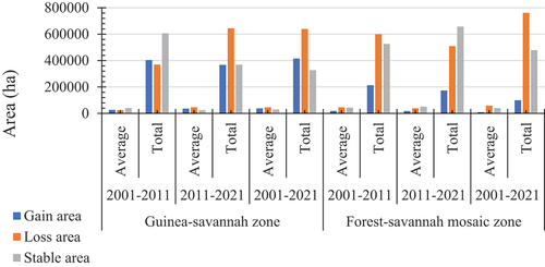
The overall analysis of the results on changes in the Forest-savannah mosaic and Guinea-savannah during 2001–2021 shows that the vegetation cover is undergoing considerable dynamism leading to considerable loss of habitable areas without obscuring the agricultural areas (Figure 14). The changes observed on both sides are not of the same magnitude (Figure 8). Considering the decades, the last one (2011–2021) has seen more loss in the Guinea-savannah zone (644232.8 ha or on average 46,016.6 ha) than in the Forest-savannah mosaic zone (508899.6 ha or on average 39,146.1 ha). However, over the whole period considered (2001–2021), the Forest-savannah zone recorded more loss in vegetation cover (761693.6 ha or an average of 58,591.8 ha). The first decade was marked by more stability in the Guinea-savannah zone (605801.3 ha or an average of 40,386.8 ha) than in the Forest-savannah mosaic zone (525933.0 ha or an average of 43,827.8 ha), but the overall trend (2001–2021) shows more pronounced stability in the Forest-savannah zone (478930.1 ha or 39,910.8 ha). However, the gains are less in this zone (99407.2 ha or an average of 9037.0 ha) over the whole period 2001–2021, compared to the Guinea-savannah zone (415377.6 ha or an average of 36,694.2 ha).

Figure 14. Comparative graph of changes obtained in the two ecological zones (Guinea-savannah and Forest-savannah mosaic).

Discussion

LULC in Guinea-savannah and Forest-savannah mosaic zone

The LULC maps obtained after classification in the two study areas showed accuracies that allowed us to carry out comparative analyses and to evaluate the vegetation dynamics in these different ecological zones that are under pressure from degradation factors at various levels of their component. Thus, the overall accuracies obtained for the classifications are respectively 93% (2001), 88% (2011), 91% (2021) for the Guinea-Savannah zone and 91% (2001), 93% (2011), 96% (2021) for the Forest-savannah zone while the values obtained for the Kappa coefficients are 91% (2001), 85%(2011), 89%(2021) for Guinea-savannah zone and 88%(2001), 89%(2011), 93%(2021). These values are consistent with those obtained through similar research in the African and West African savannah zones (Dahan et al., 2021; Koubodana et al., 2019; Li et al., 2022; Mungai et al., 2022; Nkomeje, 2017) in Ghana (Agariga et al., 2021; Amproche et al., 2020; Ghansah et al., 2022) as well as in intertropical forest areas (Allouche et al., 2006; Dan et al., 2016; Gessesse et al., 2015; Wang et al., 2022), thus meeting the Landis and Koch (1977) classification standard

Vegetal dynamics within ecological zones (Guinea-savannah and Forest-savannah zone)

The vegetation dynamics in the Guinea-Savannah zone from the results show non-uniform changes, i.e. the majority of the LULCs are in perpetual dynamism which shows that the zone is disturbed in time and space under the pressure of several parameters confirmed by several previous pieces of research due to the dynamism of the land-use units in the research districts of the ecological zone under investigation (Abubakari et al., 2022; Adanu et al., 2013). As a result, Bare soil and Built-up is the most expansive LULC unit in time and space in general. This could be due to the increasing population of the area (Ghana Statistical Service, 2021) on the one hand and the other hand the continuous degradation of the vegetation continuum leaving some areas virtually bare, e.g. areas where rocks are scoured and leached and other practices such as charcoal making (Anang et al., 2011; Obiri et al., 2014). Most of the said area is under deforestation pressure due to energy demand (charcoal production) by the local population and indeed the whole of Ghana. This leads to the felling of trees to satisfy vital needs (food preparation, charcoal). These facts will be the cause of the increase of Degraded woodland and Tree-savannah mosaic zones because according to the land realities, these units mostly overlap with the Cropland. These results confirm previous findings from northern and central Ghana in the savannah zones (Ampim et al., 2021; Braimoh & Vlek, 2005; Murray et al., 2017). While some of these LULCs (degraded woodland, Tree-savannah mosaic) have increased in the area, indicating the level of degradation, Dense woodland has also increased in the area overall. This could be due to the presence of Mole Park which is receiving special attention as a protected area contributing to ecotourism (ecosystem values) not only for the district it belongs to but for the whole of Ghana (Mohammed, 2015; Murray et al., 2017; Obeng et al., 2021). It is noted that the two districts that are considered in the ecological zone do not enjoy the same ecological and climatic conditions even though they enjoy virtually the same biophysical conditions (Gómez-Dans et al., 2022). This indicates the presence of a denser vegetative zone in the southwestern district of the zone (West Gonja) than in the northeastern district (West Mamprusi). These realities are revealed in the results if we consider our observation at the district level as the West Mamprusi side showed a clearer degradation than the West Gonja side. The objective of an overall assessment of the areas of gain, loss and stability was achieved as it was found that the areas of loss in terms of degradation of vegetation cover and deforestation are more confirmable than the areas of gain. This is a crucial issue that has also been revealed in other research that relates to the overall trend of forest resource degradation in Ghana (Acheampong et al., 2019; Dixon et al., 1996; Kyere-Boateng & Marek, 2021, 2021). In addition to the anthropogenic factors that are major causes of degradation and deforestation, the increasingly obsolete climatic factors are contributing immeasurably to this degradation today (Abbam et al., 2018; Asante & Amuakwa-Mensah, 2014; Dixon et al., 1996; Nunes et al., 2021), and these districts in the study area are among the most vulnerable areas in Ghana (Stanturf et al., 2011). These factors, together with environmental parameters closely related to climatic parameters increase other risks such as wildfires and floods. The latter, namely environmental, are still contributors to the degradation of vegetation cover (Adanu et al., 2013). The observed losses have been more in the last decade (2011–2021) than the first (2001–2011) which may be due to climatic conditions in the northern region of Ghana in recent years (Abbam et al., 2018; Dahan et al., 2023) leading to limited tree regeneration after water stress. However, the major cause is anthropogenic activities and urbanisation.

On the other hand, in the homologous zone (Forest-savannah mosaic zone), there is an increase in the areas of loss, but more considerable in terms of surface area, compared to the Guinnea-savannah zone, without taking too much account of the richness in terms of biological diversity (biotic and abiotic reality), the surface area and also the conditions of proximity with the metropolis (Accra). This zone is undergoing an increasing degradation of its resources. The Forest-Savannah Mosaic Zone, which is a richer zone in terms of biological diversity (Attuquayefio, 2008; MESTI, 2016), is considered the granary of Ghana (Titriku, 1999), providing the majority of the primary resources (food crops). This would be the cause of accelerated degradation of these natural resources and would promote soil degradation (soil impoverishment through leaching). Focusing on the Sene and Afram Plains districts, the results show that the Dense forest has suffered more from anthropic pressure, increasing the Forest-savannah mosaic, which shows a progressive fragmentation of the areas considered as Dense. This degradation is explained by the harsh conditions in the area, pushing the local population to resort to natural resources for their survival, as well as the invasion of the area by settler farmers more and more (Acheampong et al., 2019; Afikorah-Danquah, 1997, 1997; Amankwah et al., 2021; Ghana Statistical Service, 2005; Kyere-Boateng & Marek, 2021) This area, which is rich in certain forest species such as Millicia excelsa and Ceiba pentandra (the most cut), is being stripped of these species and is thus losing its natural forest-savannah characteristics and tending towards pure savannah. It should also be noted that charcoal production and logging companies (Westerhoff & Smit, 2009) observed in the area are among the activities contributing to this vegetation dynamic (Nketiah & Asante, 2018; Obiri et al., 2014). The districts considered in this ecological zone in previous research reveal how vulnerable they are to climate change (Codjoe & Owusu, 2011; Anthony & Rob, 2014). These realities further contribute to the degradation of natural resources and more specifically forestry. Statements from the local population mention the presence of vegetation fire during almost the entire dry period, which burns existing forest areas or even weakens the undergrowth. All this weakens the forest species and would be the basis of their capacity to develop in time and space. However, even though the Guinea-Savannah zone has experienced more loss and gain than the Guinea-Savannah zone over the period under consideration, it is more observed in the first decade (2001–22021) than in the second (2011–2021). This could be due to the protection and awareness programmes on the ground through non-state initiatives (NGOs) that have been observed on the ground. The observation of overall gains during the period 2001–2011 could also be due to the presence of Digya National Park in Sene District which is increasingly degraded (Ayivor et al., 2013; Twumasi et al., 2005) with the repeated passage of fires each dry season and other anthropogenic factors.

Degradation Intensity analysis

The rate or pace of LULC degradation in both study areas was observed more in Bare soil and Built-up (Guinea-savannah zone), Degraded woodland and Cropland (Forest-savannah mosaic zone) in terms of gain and Dense woodland, Cropland (Guinea-savannah zone), Dense woodland, Forest-savannah mosaic, Degraded woodland Water and wetland (Forest-savannah mosaic zone) in terms of loss. However, the intensity remains active for Dense woodland in both zones but the rate of degradation in the Forest-savannah mosaic zone is very high. This could be due to the presence of pressure on the different planes mentioned above by the presence of more and more degradation factors.

Some of the results obtained may not be consistent with the rate or intensity observed at Cropland in terms of loss in the Guinea-Savannah area. This may be due to possible errors in the LULC data used for the analysis (Pontius, 2019b; Pontius & Santacruz, 2014a). Also, the cause could be that Bare soil and Built-up, Cropland, forest land and other vegetation are often confused with each other (CILSS, 2016). According to Aldwaik and Pontius (2013), map errors can be explained by excessive/underestimated extrapolation of the three components of difference, namely quantity change, exchange and offset, which may be due to either the classification of a given category with narrow reflectance or to a wider reflectance than that observed on the ground, due in particular to the fact that at the time of the elaboration of the LULC data, historical ground truth information of the area may be absent and the elaboration of the map had to rely only on historical maps for validation (CILSS, 2016). It should be noted that quantity change is the most observed component overall in degradation intensity. This change characterised by the conversion of LULCs into other categories (e.g. Dense woodland to Bare soil and built-up) sheds light on the effective presence of advanced dynamism within LULCs and consequently, the degradation of vegetation cover in these areas. However, compared to artificial water bodies they are generally not sustainable as they are often abandoned and replaced by other categories of LULCs (Hausermann, 2018; Koua et al., 2019; Niel et al., 2005; Obour et al., 2016; Santé et al., 2019; Yankson et al., 2018), but this is not the case in our study areas because we observe a gain intensity in the Guinea-savannah zone, even if it is dormant, due to the creation of small dams by the population because of water problems in the said zone. On the other hand, the Forest-savannah mosaic zone is experiencing an active intensity of loss, which is due to intensive exploitation, degradation of the vegetative crown around the water body (Lake Ghana) and crumbling of the water body.

Conclusion

The present study implemented in an ecological zone that is homologous in terms of proximity and that enjoys practically identical ecological realities, has as its main goal to make a comparative analytical study on the evolution and degradation of their different vegetation cover in time and space so that decision-makers can reorient conservation, management, use and protection policies. For this purpose, modern processing methods such as GIS and remote sensing were used as well as quantitative analysis approaches based on mathematical tools and models through PontiusMatrix 42. The final result of this research is that the forest areas are very dynamic in the two ecological zones. The net amounts of change dominate the entire study period considered (2001-2021). Also, the Bare soil and Built-up recorded a large area in the year 2021 demonstrating the extent to which resources are under anthropogenic pressure. However, Guinea-Savannah has seen a significant increase in its agricultural area. Overall, attention should be paid to the degradation of resources that contribute to limiting or countering the phenomenon of desertification, as the loss of vegetation cover in both areas remains significant. Moreover, the intensity of degradation is active in forest areas as well as in urbanised areas. Thus, particular attention should be paid through policies and development plans to the Forest-Savannah mosaic zone to reduce or fight against the current rate of degradation. Among other things, as a preventive approach, it is necessary to intensify the monitoring of forest resources, to increase the repressive measures against the setting of vegetation fires. The local organisations for the conservation of natural resources must be restructured. Education on the importance and maintenance of the forest patrimony of these ecological zones must be taken into account as well, especially in the FSZ since it is becoming more and more threatened.

Acknowledgments

This research was made possible through funding support from the Islamic Development Bank (IsDB). The authors are particularly grateful to the University for Development Studies, West African Center for Water, Irrigation and Sustainable Agriculture (WACWISA) for providing logistics to facilitate the completion of this paper.

Disclosure statement

No potential conflict of interest was reported by the author(s).

Data availability statement

Data used in this paper are available as polygon shapefiles and some Excel sheets with data as well at https://doi.org/10.5281/zenodo.7182666

Additional information

Funding

This research was made possible through funding support from the Islamic Development Bank (IsDB).

References

- Abbam, T., Johnson, F. A., Dash, J., & Padmadas, S. S. (2018). Spatiotemporal variations in rainfall and temperature in Ghana over the twentieth century, 1900-2014. Earth & Space Science, 5(4), 120–132. https://doi.org/10.1002/2017EA000327
- Abubakari, M. M., Anaman, K. A., & Ahene-Codjoe, A. A. (2022). Urbanization and Arable land use in northern Ghana: A case study of the Sagnarigu municipality in the greater tamale area. Applied Economics and Finance, 9(1), 68. https://doi.org/10.11114/aef.v9i1.5469
- Acheampong, E. O., Macgregor, C. J., Sloan, S., & Sayer, J. (2019). Deforestation is driven by agricultural expansion in Ghana’s forest reserves. Scientific African, 5, e00146. https://doi.org/10.1016/j.sciaf.2019.e00146
- Acheampong, M., Yu, Q., Enomah, L. D., Anchang, J., & Eduful, M. (2018). Land use/cover change in Ghana’s oil city: Assessing the impact of neoliberal economic policies and implications for sustainable development goal number one–A remote sensing and GIS approach. Land Use Policy, 73, 373–384. https://doi.org/10.1016/j.landusepol.2018.02.019
- Adanu, S. K., Mensah, F. K., & Adanu, S. K. (2013). Enhancing Environmental Integrity in the northern savanna zone of Ghana: A Remote Sensing and GIS approach. Journal of Environment and Earth Science, 3(5), 67–77.
- Addae, B., & Oppelt, N. (2019). Land-use/land-cover change analysis and urban growth modelling in the greater Accra metropolitan area (GAMA), Ghana. Urban Science, 3(1), 26. https://doi.org/10.3390/urbansci3010026
- Adjei, P. O.-W., Buor, D., & Addrah, P. (2014). Geo-spatial analysis of land use and land cover changes in the Lake bosomtwe basin of Ghana. Ghana Journal Geogr, 6, 1–23.
- Aduah, M. S., & Baffoe, P. E. (2013). Remote sensing for mapping land-use/cover changes and urban sprawl in Sekon-di-Takoradi, Western region of Ghana. International Journal of Engineering Science, 2(10), 66–72.
- Afikorah-Danquah, S. (1997). Local resource management in the Forest-savanna transition zone: The case of Wenchi district, Ghana. IDS Bulletin, 28(4), 36–46. https://doi.org/10.1111/j.1759-5436.1997.mp28004005.x
- Agariga, F., Abugre, S., & Appiah, M. (2021). Spatio-temporal changes in land use and forest cover in the Asutifi North district of Ahafo region of Ghana, (1986–2020). Environmental Challenges, 5, 100209. https://doi.org/10.1016/j.envc.2021.100209
- Aldwaik, S. Z., Jeffrey, A. O., & Pontius Jr, R. G., Jr. (2015). Behavior-based aggregation of land categories for temporal change analysis, International Journal of Applied Earth Observation and Geoinformation, 35(B), 229–238. https://doi.org/10.1016/j.jag.2014.09.007
- Aldwaik, S. Z., & Pontius, R. G., Jr. (2012). Intensity analysis to unify measurements of size and stationarity of land changes by interval, category, and transition. Landscape and Urban Planning, 106(1), 103–114. https://doi.org/10.1016/j.landurbplan.2012.02.010
- Aldwaik, S. Z., & Pontius, R. G., Jr. (2013). Map errors that could account for deviations from a uniform intensity of land change. International Journal of Geographical Information Science, 27(9), 1717–1739. https://doi.org/10.1080/13658816.2013.787618
- Allouche, O., Tsoar, A., & Kadmon, R. (2006). Assessing the accuracy of species distribution models: Prevalence, kappa and the true skill statistic (TSS): Assessing the accuracy of distribution models. Journal of Applied Ecology, 43(6), 1223–1232. https://doi.org/10.1111/j.1365-2664.2006.01214.x
- Alo, C. A., & Pontius, R. G., Jr. (2008). Identifying systematic land-cover transitions using Remote Sensing and GIS: The fate of forests inside and outside protected areas of Southwestern Ghana. Environment and Planning B: Planning and Design, 35(2), 280–295. https://doi.org/10.1068/b32091
- Amankwah, A. A., Quaye-Ballard, J. A., Koomson, B., Amankwah, R. K., Awotwi, A., Kankam, B. O., Opuni-Frimpong, N. Y., Baah, D. S., & Adu-Bredu, S. (2021). Deforestation in the forest-savannah transition zone of Ghana: Boabeng-Fiema monkey sanctuary. Global Ecology and Conservation, 25, e01440. https://doi.org/10.1016/j.gecco.2020.e01440
- Ampim, P. A. Y., Ogbe, M., Obeng, E., Akley, E. K., & MacCarthy, D. S. (2021). Land cover changes in Ghana over the Past 24 years. Sustainability, 13(9), 4951. https://doi.org/10.3390/su13094951
- Amproche, A. A., Antwi, M., & Kabo-Bah, A. T. (2020). Geospatial assessment of land use and land cover patterns in the black Volta Basin, Ghana. Journal of Remote Sensing &, 09(1). GIS, 09(01. https://doi.org/10.35248/2469-4134.20.9.269
- Anang, B. T., Akuriba, M. A., & Alerigesane, A. A. (2011). Charcoal production in Gushegu District, northern region, Ghana: Lessons for sustainable forest management. International Journal of Environmental Sciences, 1(7), 1944–1953.
- Angelsen, A. (2001). Deforestation–Forestation. In N. J. Smelser & B. Paul (Eds.), Baltes, International Encyclopedia of the Social & Behavioral Sciences, Pergamon (pp. 3359–3364). https://doi.org/10.1016/B0-08-043076-7/04173-5
- Anthony, N. O., & Rob, M. (2014). Climate change impact and adaptation pathways for forest dependent livelihood systems in Nigeria. African Journal of Agricultural Research, 9(24), 1819–1832.
- Asante, F., & Amuakwa-Mensah, F. (2014). Climate change and variability in Ghana: Stocktaking. Climate, 3(1), 78–99. https://doi.org/10.3390/cli3010078
- Asenso Barnieh, B., Jia, L., Menenti, M., Jiang, M., Zhou, J., Lv, Y., Zeng, Y., & Bennour, A. (2022). Quantifying spatial reallocation of land use/land cover categories in West Africa. Ecological Indicators, 135, 108556. https://doi.org/10.1016/j.ecolind.2022.108556
- Attua, E. M., & Fisher, J. B. (2011). Historical and future land-cover change in a municipality of Ghana. Earth Interactions, 15(9), 1–26. https://doi.org/10.1175/2010EI304.1
- Attuquayefio, D. K. (2008). Biodiversity assessment (Rodents and Avifauna) of five Forest reserves in theBrong-Ahafo region, Ghana. Ghana Journal of Science, 48(1), 37–45. https://doi.org/10.4314/gjs.v48i1.56252
- Ayivor, J. S., Gordon, C., & Ntiamoa-Baidu, Y. (2013). Protected area management and livelihood conflicts in Ghana: A case study of Digya National Park. PARKS, 19(1), 37–50. https://doi.org/10.2305/IUCN.CH.2013.PARKS-19-1.JSA.en
- Ayivor, J. S., Pabi, O., Ofori, B. D., Yirenya-Taiwiah, D. R., & Gordon, C. (2015). Agro-diversity in the Forest-savannah transition zone of Ghana: A strategy for food security against climatic and socio-economic stressors. Environment and Natural Resources Research. https://doi.org/10.5539/enrr.v6n1p1
- Bai, Z. G., Dent, D. L., Olsson, L., & Schaepman, M. E. (2008). Proxy global assessment of land degradation. Soil Use Manage, 24(3), 223–234. https://doi.org/10.1111/j.1475-2743.2008.00169.x
- Ben-Michael, E., Feller, A., & Rothstein, J. (2022, April). Synthetic controls with staggered adoption. Journal of the Royal Statistical Society Series B, Statistical Methodology, 84(2), 351–381. https://doi.org/10.1111/rssb.12448
- Bessah, E., Bala, A., Agodzo, S. K., Okhimamhe, A. A., Boakye, E. A., & Ibrahim, S. U. (2019). The impact of crop farmers’ decisions on future land use, land cover changes in Kintampo North Municipality of Ghana. International Journal of Climate Change Strategies and Management, 11(1), 72–87. https://doi.org/10.1108/IJCCSM-05-2017-0114
- Braimoh, A. K. (2004). Seasonal migration and land-use change in Ghana. Land Degrad. Land Degradation & Development, 15(1), 37–47. https://doi.org/10.1002/ldr.588
- Braimoh, A. K., & Vlek, P. L. G. (2005). Land-cover change Trajectories in northern Ghana. Environmental Management, 36(3), 356–373. https://doi.org/10.1007/s00267-004-0283-7
- CILSS. (2016). Landscapes of West Africa – a Window on a Changing world. U.S. Geological Survey EROS, 47914 252nd St, Garretson, SD 57030. UNITED STATES.
- Codjoe, S. N. A., & Owusu, G. (2011). Climate change/variability and food systems: Evidence from the Afram Plains, Ghana. Regional Environmental Change, 11(4), 753–765. https://doi.org/10.1007/s10113-011-0211-3
- Curtis, P. G., Slay, C. M., Harris, N. L., Tyukavina, A., & Hansen, M. C. (2018). Classifying drivers of global forest loss. Science, 361(6407), 1108–1111. https://doi.org/10.1126/science.aau3445
- Dahan, K. S., Kasei, R. A., Husseini, R., Said, M. Y., & Rahman, M. M. (2023). Towards understanding the environmental and climatic changes and its contribution to the spread of wildfires in Ghana using remote sensing tools and machine learning (Google Earth Engine). International Journal of Digital Earth, 16(1), 1300–1331. https://doi.org/10.1080/17538947.2023.2197263
- Dahan, K. S., N’da, D. H., & Kaudjhis, C. (2021). Dynamique spatio-temporelle des feux de 2001 à 2019 et dégradation du couvert végétal en zone de contact foret-savane, Département de Toumodi, Centre de la Côte d’Ivoire. Afrique Science Revue Internationale Des Sciences et Technologie, 19(2), 94–113.
- Dan, T. T., Chen, C. F., Chiang, S. H., & Ogawa, S. (2016). Mapping and change analysis in mangrove forest by using Landsat imagery. ISPRS Annals of Photogrammetry, Remote Sensing & Spatial Information Sciences, 8, 109–116. https://doi.org/10.5194/isprsannals-III-8-109-2016
- Davey, S. M., & Sarre, A. (2020). Editorial: The 2019/20 black summer bushfires. Australian Forestry, 83(2), 47–51. https://doi.org/10.1080/00049158.2020.1769899
- Derouin, S. (2019). Deforestation: Causes & effects. livescience.com/27692-deforestation.html (Retrieved September 12th, 2022).
- Dixon, R., Perry, J., Vanderklein, E., & Hiol Hiol, F. (1996). Vulnerability of forest resources to global climate change: Case study of Cameroon and Ghana. Climate Research, 6, 127–133. https://doi.org/10.3354/cr006127
- Doshvarpassand, S., & Wang, X. (2021). An automated pipeline for dynamic detection of sub-surface metal loss defects across cold thermography images. Sensors, 21(14), 4811. https://doi.org/10.3390/s21144811
- Eckhardt, B. W., & Moore, T. R. (1990). Controls on dissolved organicc carbon concentrations in streams, southern Quebec. Canadian Journal of Fisheries and Aquatic Sciences, 47, 1537–1544.
- Ekumah, B., Armah, F. A., Afrifa, E. K. A., Aheto, D. W., Odoi, J. O., & Afitiri, A.-R. (2020). Assessing land use and land cover change in coastal urban wetlands of international importance in Ghana using intensity analysis. Wetlands Ecology and Management, 28(2), 271–284. https://doi.org/10.1007/s11273-020-09712-5
- Enaruvbe, G. O., & Pontius, R. G., Jr. (2015, January). Influence of classification errors on intensity analysis of land changes in southern Nigeria. International Journal of Remote, 36(1), 244–261. https://doi.org/10.1080/01431161.2014.994721
- Eswaran, H., Lal, R., & Reich, P. F. (2001). Land degradation: An overview. In: Responses to Land Degradation, Eds. E. M. Bridges, I. D. Hannam, L. R. Olderman, F. W. T. Penning de Vries, S. J. Scherr, & S. Sompatpanit. Proc. of the 2nd International Conference on Land Degradation and Desertification, KonKaen, Thailand. New Delhi, India: Oxford Press.
- FAO. (2022). The state of the world’s forests 2022. Forest pathways for green recovery and building inclusive, resilient and sustainable economies. https://doi.org/10.4060/cb9360en
- Gaveau, D. L., Pirard, R., Salim, M. A., Tonoto, P., Yaen, H., Parks, S. A., & Carmenta, R. (2017). Overlapping land claims limit the use of satellites to monitor no‐deforestation commitments and no‐burning compliance. Conservation Letters, 10(2), 257–264. https://doi.org/10.1111/conl.12256
- Gessesse, B., Bewket, W., & Bräuning, A. (2015). Why does accuracy assessment and validation of multi-resolution-based satellite image classification matter? A methodological discourse. SINET: Ethiopian Journal of Science, 38(1), 29–42.
- Ghana Statistical Service, (2005). Population data analysis reports. Vol 1: Socioeconomic and demographic trends analysis,
- Ghana Statistical Service. (2021) PHC general report Vol 3A_Population of regions and Districts_181121.Pdf POPULATION of REGIONS and DISTRICTS REPORT (statsghana.Gov.gh)
- Ghana Statistics Service 2013. (2010). Population & housing census: National analytical report; Ghana Statistics Service:
- Ghansah, B., Foster, T., Higginbottom, T. P., Adhikari, R., & Zwart, S. J. (2022). Monitoring spatial-temporal variations of surface areas of small reservoirs in Ghana’s Upper East region using Sentinel-2 satellite imagery and machine learning. Elsevier Enhanced Reader, 125, 103082. https://doi.org/10.1016/j.pce.2021.103082
- Gockowski, J., Afari-Sefa, V., Sarpong, D. B., Osei-Asare, Y. B., & Dziwornu, A. K. (2011). Increasing income of Ghanaian cocoa farmers: Is introduction of fine flavour cocoa a viable alternative. Quarterly Journal of International Agriculture, 50, 175–200.
- Gómez-Dans, J. L., Lewis, P. E., Yin, F., Asare, K., Lamptey, P., Aidoo, K. K. Y., MacCarthy, D., Ma, H., Wu, Q., Addi, M., Aboagye-Ntow, S., Doe, C. E., Alhassan, R., Kankam-Boadu, I., Huang, J., & Li, X. (2022). Location, biophysical and agronomic parameters for croplands in northern Ghana. [Preprint]. ESSD – Land/Land Cover and Land Use. https://doi.org/10.5194/essd-2022-256
- Hausermann, H. (2018). “Ghana must progress, but we are really suffering”: Bui Dam, antipolitics Development, and the livelihood implications for rural people. Society & Natural Resources, 31(6), 633–648. https://doi.org/10.1080/08941920.2017.1422062
- Koranteng, A., Adu-Poku, I., & Zawiła-Niedźwiecki, T. (2019). Landuse and land cover dynamics in the Volta River Basin surrounding APSD forest plantation, Ghana. Folia Forestalia Polonica, 61(1), 78–89. https://doi.org/10.2478/ffp-2019-0008
- Koua, J. T., Anoh, A. K., Soro, D. T., Kouame, J. K., Jean, R., & Jourda, P. (2019). Evaluation of agricultural practices scenarios for reducing erosion in buyo lake catchment (Sassandra; Côte d’Ivoire) by use of GIS. Journal of Geoscience and Environment Protection, 7(7), 154–171. https://doi.org/10.4236/gep.2019.77011
- Koubodana, H., Diekkrüger, D., Näschen, B., Adounkpe, K., & Atchonouglo, K. (2019). Impact of the accuracy of land cover data sets on the accuracy of land cover change scenarios in the Mono River Basin, Togo, West Africa. International Journal of Advanced Remote Sensing and GIS, 8. https://doi.org/10.20944/preprints201906.0143.v1
- Kroeger, A., Bakhtary, H., Haupt, F., & Streck, C. (2017). Eliminating deforestation from the cocoa Supply Chain. World Bank. https://doi.org/10.1596/26549
- Kyere-Boateng, R., & Marek, M. V. (2021). Analysis of the social-ecological causes of deforestation and Forest degradation in Ghana: Application of the DPSIR framework. Forests, 12(4), 409. https://doi.org/10.3390/f12040409
- Landis, J. R., & Koch, G. G. (1977). The measurement of observer agreement for categorical data biometrics. Biometrics, 1(1), 159–174. https://doi.org/10.2307/2529310
- Li, C., Dash, J., Asamoah, M., Sheffield, J., Dzodzomenyo, M., Gebrechorkos, S. H., Anghileri, D., & Wright, J. (2022). Increased flooded area and exposure in the White Volta river basin in Western Africa, identified from multi-source remote sensing data. Scientific Reports, 12(1), 3701. https://doi.org/10.1038/s41598-022-07720-4
- Li, C. K., Fang, W., & Dong, X. J. (2015). Research on the classification of high resolution image based on object-oriented and class rule. The International Archives of the Photogrammetry, Remote Sensing and Spatial Information Sciences, XL-7/W4, 75–80. https://doi.org/10.5194/isprsarchives-XL-7-W4-75-2015
- Lillesand, T., Kiefer, R. W., & Chipman, J. (Eds). (2014). Remote sensing and image interpretation. John Wiley & Sons.
- Li, J., & Roy, D. P. (2017). A global analysis of sentinel-2a, sentinel-2b and Landsat-8 data revisit intervals and implications for terrestrial monitoring. Remote Sensing, 9(9), 902. https://doi.org/10.3390/rs9090902
- Manandhar, R., Odeh, I. O. A., & Pontius, R. G., Jr. (2009). Analysis of twenty years of categorical land transitions in the Lower Hunter. Agriculture, Ecosystems and Environment, 135(4), 336–346. https://doi.org/10.1016/j.agee.2009.10.016
- Martínez, J., Vega-Garcia, C., & Chuvieco, E. (2009). Human-caused wildfire risk rating for prevention planning in Spain. Journal of Environmental Management, 90(2), 1241–1252.
- Menczer, K., & Quaye, E. (2006). Usaid/ghana environmental threats and opportunities assessment. (FAA 118/9 Assessment). US Agency for International Development. Available online at: https://pdf.usaid.gov/pdf_docs/PA00JXBB.pdf
- MESTI, Ministry of Environment, Science, Technology, and Innovation. (2016). National biodiversity strategy and action plan. https://www.cbd.int/doc/world/gh/gh-nbsap-v2-en.pdf
- MOFA Ministry of Food & Agriculture. (2015). Kassena-Nankana West. https://mofa.gov.gh/site/sports/district-directorates/upper-east-region/267-kassena-nankana-west (Accessed 25 November 2021).
- Mohammed, I. (2015). Terrestrial protected areas and Poverty Reduction in Ghana: A case study of the Mole National Park and the Mognori and Murugu communities. Journal of Sustainable Development Studies, 8(1), 129–192.
- Muchena, F. N. (2008). Indicators for sustainable land management in Kenya’s context. GEF land degradation focal area indicators. East Africa: Nairobi.
- Mundia, C. N., & Aniya, M. (2005). ``analysis of land use/cover changes and urban expansion of Nairobi city using remote sensing and GIS’’. International Journal of Remote Sensing, 26(13), 2831–2849. https://doi.org/10.1080/01431160500117865
- Mungai, L. M., Messina, J. P., Zulu, L. C., Qi, J., & Snapp, S. (2022). Modelling spatiotemporal patterns of land use/land cover change in central Malawi using a Neural Network Model. Remote Sensing, 14(14), 3477. https://doi.org/10.3390/rs14143477
- Murray, L., Sidman, G., Grais, A., Bernal, B., Pearson, T., & Sohngen, B. (2017). Northern Ghana land use ecosystem Service and economic valuation study. 52.
- Myers, N. (1992). The primary source: Tropical forests and our future. https://doi.org/10.1007/978-94-017-3608-4
- N’Da, D. H., E, N. K., Waddja, E. M., & Affian, K. (2008). Apport de la télédétection au suivi de la déforestation dans le Parc National de la Marahoué (Côte d’Ivoire). Télédétection, 8(1), 17–34.
- Niel, H., Leduc, C., & Dieulin, C. (2005). Caractérisation de la Variabilité Spatiale et Temporelle des Précipitations Annuelles sur le Bassin du Lac Tchad au Cours du 20ème Siècle/Spatial and Temporal Variability of Annual Rainfall in the Lake Chad Basin During the 20th Century. Hydrological Sciences Journal, 50(2), 223–243. https://doi.org/10.1623/hysj.50.2.223.61800
- Nindel, S. (2017). Forest fire dynamics and carbon stocks in different ecological zones of Ghana. Dissertation, Dresden University of Technology, Available online at: https://tud.qucosa.de/api/qucosa%3A31173/attachment/ATT-0/
- Nketiah, K. S., & Asante, J. (2018). Estimating national charcoal production in Ghana. Ghana: Tropenbos.
- Nkomeje, F. (2017). Comparative performance of multi-source reference data to assess the accuracy of classified remotely sensed imagery: Example of landsat 8 OLI across Kigali city-rwanda 2015. International Journal of Engineering Works, 4(1), 10–20.
- Nunes, L. J. R., Meireles, C. I. R., Gomes, C. J. P., & Ribeiro, N. M. C. A. (2021). The impact of climate change on Forest Development: A sustainable approach to management models applied to Mediterranean-type climate regions. Plants, 11(1), 69. https://doi.org/10.3390/plants11010069
- Obeng, E. A., Dakurah, I., Oduro, K. A., & Obiri, B. D. (2021). Local communities’ preferences and economic values for ecosystem services from Mole National Park in Ghana: A choice experiment approach. Global Ecology and Conservation, 32, e01904. https://doi.org/10.1016/j.gecco.2021.e01904
- Obiri, B. D., Nunoo, I., Obeng, E., Owusu, F. W., & Marfo, E. (2014). The charcoal industry in Ghana: An alternative livelihood option for displaced illegal chainsaw lumber producers. Tropenbos International.
- Obour, P. B., Owusu, K., Agyeman, E. A., Ahenkan, A., & Madrid, A. N. (2016). The impacts of dams on local livelihoods: A study of the Bui Hydroelectric Project in Ghana. International Journal of Water Resources Development, 32(2), 286–300. https://doi.org/10.1080/07900627.2015.1022892
- Pirotti, F., Sunar, F., & Piragnolo, M. (2016). Benchmark of machine learning methods for classification of a sentinel-2 image. The International Archives of the Photogrammetry, Remote Sensing and Spatial Information Sciences, XLI-B7, 335–340. https://doi.org/10.5194/isprs-archives-XLI-B7-335-2016
- Pontius, R. G., Jr. (2019a). Component intensities to relate difference by category with difference overall. International Journal of Applied Earth Observation and Geoinformation, July 2018 77, 94–99. https://doi.org/10.1016/j.jag.2018.07.024.
- Pontius, R. G., Jr. (2019b). Component intensities to relate difference by category with difference overall. International Journal of Applied Earth Observations & Geoinformation, 77, 94–99. https://doi.org/10.1016/j.jag.2018.07.024
- Pontius, R. G., Jr., & Millones, M. (2011). Death to Kappa: Birth of quantity disagreement and allocation disagreement for accuracy assessment. International Journal of Remote Sensing, 32(15), 4407–4429. https://doi.org/10.1080/01431161.2011.552923
- Pontius, R. G., Jr., & Santacruz, A. (2014a, November). Quantity, exchange, and shift components of difference in a square contingency table. International Journal of Remote Sensing, 35(21), 7543–7554. https://doi.org/10.1080/2150704X.2014.969814
- Pontius, R. G., Jr., & Santacruz, A. (2014b). Quantity, exchange and shift components of differences in a Square contingency table. International Journal of Remote Sensing, 35(21), 7543–7554. https://doi.org/10.1080/2150704X.2014.969814
- Quan, B., Pontius, R. G., Jr., & Song, H., (2019). Intensity analysis to communicate land change during three time intervals in two regions of Quanzhou city, China two regions of Quanzhou city, China. GIScience & Remote Sensing 1–16. https://doi.org/10.1080/15481603.2019.1658420.
- Quan, B., Pontius, R. G., & Song, H. (2020). Intensity analysis to communicate land change during three time intervals in two regions of Quanzhou city, China. GIScience & Remote Sensing, 57(1), 21–36. https://doi.org/10.1080/15481603.2019.1658420
- Rahman & Dedieu. (1994). SMAC: A simplified method for atmospheric correction of satellite measurements in the solar spectrum. International Journal of Remote Sensing, 15(1). https://doi.org/10.1080/01431169408954055
- Reid, W. V., Mooney, H. A., Cropper, A., Capistrano, D., Carpenter, S. R., Chopra, K. … & Zurek, M. B. (2005). Ecosystems and human well-being—Synthesis: A report of the Millennium ecosystem assessment. Island Press. https://edepot.wur.nl/45159.
- Reynolds, J. F., & Smith, D. M. S. (2002). Global desertification—do humans cause deserts? Dahlem Workshop Report 88. Dahlem University Press.
- Rouse, J. W., Haas, R. H., Schell, J. A., & Deering, D. W. (1974). Monitoring vegetation systems in the Great Plains with ERTS. NASA Spec. Publ, 351, 309.
- Rwanga, S., & Ndambuki, J. (2017). Accuracy assessment of land use/land cover classification using Remote Sensing and GIS. International Journal of Geosciences, 8(04), 611–622. https://doi.org/10.4236/ijg.2017.84033
- Safriel, U. N. (2007). The assessment of global trends in land degradation. In Sivakumar, M. V. K. and Ndiang’ui, N. Climate and Land Degradation (ed, pp. 1–38). Springer Verlag. https://doi.org/10.1007/978-3-540-72438-4_1
- Sands, R. (2005). Forestry in a Global context. CABI Publishing. https://doi.org/10.1079/9780851990897.0001
- Santé, N., Go, Y. A. N., Soro, G. E., Meledje, N. D. H., & Ti, B. (2019). Characterization of meteorological droughts occurrences in C ˆ o te d ’ Ivoire: Case of the sassandra watershed. Climate, 7(4), 60. https://doi.org/10.3390/cli7040060
- Shoyama, K., Braimoh, A. K., Avtar, R., & Saito, O. (2018). Land transition and intensity analysis of Cropland expansion in northern Ghana. Environmental Management, 62(5), 892–905. https://doi.org/10.1007/s00267-018-1085-7
- Simonetti, D., Marelli, A., & Eva, H. D. (2015). IMPACT: Portable GIS toolbox image processing and land cover mapping. Publications Office of the European Union, EUR 27358 EN. https://publications.jrc.ec.europa.eu/repository/handle/JRC96789
- Skupinski, G., Binhtran, D., & Weber, C. (2009). Les images satellites Spot multi-dates et la métrique spatiale dans l’étude du changement urbain et suburbain - Le cas de la basse vallée de la Bruche (BasRhin, France. Cybergeo: European Journal of Geography. article, N°439, DOI:10.4000/cybergeo.21995. 10.4000/cybergeo.21995
- Song, X., Yang, C., Wu, M., Zhao, C., Yang, G., Hoffmann, W. C., & Huang, W. (2017). Evaluation of sentinel-2a satellite imagery for mapping cotton root rot. Remote Sensing, 9(9), 906. https://doi.org/10.3390/rs9090906
- Stanturf, J. A., Melvin, L., Warren, S. C., Jr., Polasky, S. C., Goodrick, S. L., Armah, F., & Atuahene Nyako, Y. (2011). Ghana climate change vulnerability and adaptation assessment, this report was produced for review by the United States Agency for International Development ( USAID). It was prepared by the USDA Forest Service, International Programs, 258p.
- Teferi, E., Bewket, W., Uhlenbrook, S., & Wenninger, J. (2013). Understanding recent land use and land cover dynamics in the source region of the Upper Blue Nile, Ethiopia: Spatially explicit statistical modelling of systematic transitions. Agriculture, Ecosystems & Environment, 165, 98–117. https://doi.org/10.1016/j.agee.2012.11.007
- Titriku, P. K. (1999). Agriculture in the Volta Basin: Problems and prospects. In C. Gordon & J. K. Ametekpor (Eds.), Sustainable Integrated Development of the Volta Basin VBRP (pp. 107–116). University of Ghana.
- Toure, S. I., Stow, D. A., Clarke, K., & Weeks, J. (2020). Patterns of land cover and land use change within the two major metropolitan areas of Ghana. Geocarto International, 35(2), 209–223. https://doi.org/10.1080/10106049.2018.1516244
- Twumasi, Y. A., Coleman, T. L., & Manu, A. (2005). Biodiversity management using remotely sensed data and GIS technologies: The case of Digya National Park, Ghana. In Proceedings of the 31st international symposium on Remote Sensing of Environment (ISRSE)– Global Monitoring for Sustainability and Security Conference (Paper published online and CD ROM). The International Society of Photogrammetry and Remote Sensing (ISPRS). June 20-21. Saint Petersburg, Russia Federation.
- Ukrainski, P. (2016). Classification accuracy assessment. Confusion matrix method. Retrieved from, http://www.50northspatial.org/classification-accuracy-assessment-confusion-matrix-method/on September 13, 2022.
- Vasconcelos, M. J. P., Biai, J. C. M., Arajo, A., & Diniz, M. A. (2002). Land cover change in two protected areas of Guinea-Bissau (1956-1998). Applied Geography, 22(2), 139–156. https://doi.org/10.1016/S0143-6228(02)00005-X
- Wang, X., Wang, J., Wang, W., Zhao, M., & Chaudhary, S. (2022). Consistency and accuracy Evaluation analysis of four Cropland cover products: A case study of Indochina Peninsula. Journal of Sensors, 2022, 1–25. https://doi.org/10.1155/2022/2876976
- Westerhoff, L., & Smit, B. (2009). The rains are disappointing us: Dynamic vulnerability and adaptation to multiple stressors in the Afram Plains, Ghana. Mitigation and Adaptation Strategies for Global Change, 14(4), 317–337. https://doi.org/10.1007/s11027-008-9166-1
- Wimberly, M. C., Dwomoh, F. K., Numata, I., Mensah, F., Amoako, J., Nekorchuk, D. M., & McMahon, A. (2022). Historical trends of degradation, loss, and recovery in the tropical forest reserves of Ghana. International Journal of Digital Earth, 15(1), 30–51. https://doi.org/10.1080/17538947.2021.2012533
- Yang, X., & P, L. C. (2002). ``using a time series of satellite imagery to detect land use and land cover changes in the Atlanta, Georgia metropolitan area’’. International Journal of Remote Sensing, 23(9), 1775–1798. https://doi.org/10.1080/01431160110075802
- Yankson, P. W. K., Asiedu, A. B., Owusu, K., Urban, F., & Siciliano, G. (2018). The livelihood challenges of resettled communities of the Bui Dam project in Ghana and the role of Chinese dam-builders. Development Policy Review: The Journal of the Overseas Development Institute, 36, O476–O494. https://doi.org/10.1111/dpr.12259
- Yuan, F., E, S. K., C, L. B., & E, B. M. (2005). ``land cover classification and change analysis of the Twin Cities (Minnesota) metropolitan area by multitemporal Landsat remote sensing’’. Remote Sensing of Environment, 98(2–3), 317–328. https://doi.org/10.1016/j.rse.2005.08.006
- Zaehringer, J. G., Eckert, S., & Messerli, P. (2015). Revealing Regional deforestation dynamics in North-Eastern Madagascar—Insights from multi-temporal land cover change analysis. Land, 4(2), 454–474. https://doi.org/10.3390/land4020454
- Zhang, B., Zhang, Q., Feng, C., Feng, Q., & Zhang, S. (2017). Understanding land use and land cover dynamics from 1976 to 2014 in Yellow River Delta. Land, 6(1), 20. https://doi.org/10.3390/land6010020
- Zhou, P., Huang, J., Pontius, R. G., & Hong, H. (2014). Land classification and change intensity analysis in a coastal watershed of Southeast China. Sensors (Basel), 14(7), 11640–11658. https://doi.org/10.3390/s140711640
- Ziadat, F. M., Zdruli, P., Christiansen, S., Caon, L., Monem, M. A., & Fetsi, T. (2021). An Overview of land degradation and sustainable land management in the near East and North Africa. Sustainable Agriculture Research, 11(1), 11. https://doi.org/10.5539/sar.v11n1p11