Gully-type debris flow susceptibility assessment based on a multi-channel multi-scale residual network fusing multi-source data: a case study of Nujiang Prefecture

ABSTRACT

In large-scale debris flow susceptibility assessments, there is often excessive manual intervention, low efficiency, and inadequate model accuracy. To address these issues, this paper integrates multiple data sources and proposes a Multi-channel and Multi-scale Residual Network (MMRNet) for automatic extraction of gully features. Firstly, MMRNet employs a multi-scale feature fusion module to capture both local and global features of gullies, enhancing the model’s feature representation capabilities. It then uses an improved residual structure to fuse shallow features, compress features, and improve assessment efficiency. Additionally, channel rearrangement techniques are used to enhance feature flow. Finally, susceptibility prediction is made based on the similarity between the gully under evaluation and gullies where debris flows have occurred. The natural breakpoint method is used to classify susceptibility results into five levels. Experimental results show that the very high susceptibility zones for debris flows are mainly concentrated in areas with abundant river systems along the Nujiang River, covering 61.68% of the entire study area, with a debris flow proportion of 98.78%. The MMRNet model achieves an accuracy (ACC) of 81.6% and an area under the curve (AUC) of 0.8320, indicating that this model is a high-performance method for debris flow susceptibility assessment.

KEYWORDS:

• Debris flow
• convolutional neural network
• multi-scale features
• deep learning
• machine learning

1. Introduction

Debris flow is a common geological hazard in mountainous areas. It is formed by the mixture of water with a large amount of sediment, debris, mud, and loose materials. Debris flows are characterised by their suddenness, fast flow velocity, high flow volume, large material capacity, and strong destructive potential (Jakob et al., 2005). Debris flows primarily occur in mountainous regions, plateau glacier areas, or areas with abundant water systems. These areas often have steep terrain, deep valleys, significant elevation differences, and a lack of vegetation cover on the surface, making them susceptible to water erosion. In particular, in geographically challenging and complex areas like the Nujiang Prefecture, the frequency of debris flow occurrences is relatively high. The formation of debris flows is influenced by various factors, such as earthquakes, rainfall, glacier melt, water erosion, and human activities, all of which can trigger debris flow events (Bonasera et al., 2022; Lauro et al., 2017; Takahashi, 2007; Tang et al., 2009; Yao et al., 2012). Conducting a reasonable susceptibility assessment of debris flows and implementing preventive measures in high-susceptibility debris flow areas can help reduce the losses caused by debris flows (Rodríguez-Morata et al., 2019).

At present, common methods for assessing the susceptibility to debris flows can be broadly categorised into four types: field investigation method, physical modelling method, statistical theory method, and machine learning method. Traditional susceptibility assessment of debris flows relies primarily on field investigations conducted by researchers. These assessments define susceptibility zones based on historical records and actual observations (Simoni et al., 2020). This method assists in more accurately evaluating the susceptibility to debris flows (Lombardo et al., 2016). However, due to the steep and high terrain in mountainous areas, it can be challenging for investigators to access these areas, leading to issues such as low efficiency and high risks associated with conducting large-scale field surveys. Physical modelling methods involve selecting a dynamic model for simulation and then inputting specific information about a particular gully, such as rainfall intensity and yield stress, into the model for numerical simulation. Finally, the danger of the gully is evaluated based on parameters such as flow velocity and discharge obtained from the simulation. Common methods in this category include FLO-2D (Gomes et al., 2013), FLO-3D (Kim et al., 2021), DAN3D (Choi & Kwon, 2021), Debris2D (Hsu & Liu, 2019), and others. One of the challenges with physical modelling methods is that they require data for model input, which goes beyond basic statistics like main channel length and slope. They also require data that may only be obtainable through field investigations or literature review, such as the locations of water collection points and source conditions (Romeo et al., 2023). Such data may not be readily available in literature or may be difficult to acquire in complex mountainous terrains. Consequently, these methods are often only applicable to a limited number of valleys and may not be suitable for rapidly assessing the susceptibility of hundreds of valleys. Statistical theory-based methods involve researchers using remote sensing and GIS (Geographic Information System) technology to extract terrain and geomorphic factors related to debris flows from DEM (Digital Elevation Model) and remote sensing images. They then combine statistical methods to assign weights to these influencing factors and choose appropriate functions to model the relationships between these attributes. The fitted functions are used as evaluation functions. When assessing an unknown gully, the relevant attributes of the target gully are input into the evaluation function, which yields the assessment result. Various types of statistical models have been applied to debris flow susceptibility assessment, including information value, frequency ratio, certainty factor (Dash et al., 2022), logistic regression (Wu et al., 2018), Analytic Hierarchy Process (Li et al., 2021), and grey relational analysis (Chang et al., 2014). While statistical theory-based methods are currently mainstream, they do have some limitations. The types of influencing factors need to be manually selected, and the weights of each factor need to be determined through manual calculation. The choice of influencing factors and their weights can potentially lead to significant differences in the experimental results. In recent years, machine learning-based methods for debris flow susceptibility assessment have gained popularity. These methods involve inputting predefined influencing factors into a model, tuning the model parameters, and then using the tuned model to assess debris flow susceptibility. Machine learning techniques like BP neural networks (Chang & Chao, 2006), support vector machines (Qiu et al., 2022), and random forests (Zhang et al., 2019) have been applied to debris flow susceptibility studies. However, even these machine learning methods may require manual selection of influencing factors. Machine learning methods have shown promise but still require careful consideration and manual selection of influencing factors, which can be a limitation. Nevertheless, they offer potential advantages in terms of automation and the ability to adapt to complex and large datasets.

Nowadays, the new generation of machine learning technologies, represented by Convolutional Neural Networks (CNNs), is steadily maturing and emerging as a significant player in the field of geological disasters (Chen et al., 2020; Hakim et al., 2022). In large-scale debris flow susceptibility assessments, there is often a problem of excessive manual intervention and inefficiency. Using CNNs to automatically extract image features from debris flow gullies without predefining influencing factors can reduce human intervention and provide a more objective and efficient way to delineate debris flow susceptibility zones (Xu & Wang, 2022). While CNNs offer unique advantages, there has been relatively limited research on the combination of CNNs with debris flow gully imagery. Previous studies have suffered from issues like insufficient sample data, inadequate richness in dataset features, and model accuracy.

Therefore, the main objective of this study is to construct a feature-rich dataset of debris flow gully images and develop a CNN model suitable for debris flow susceptibility assessment. By using CNN to automatically extract image features from gully images, this approach aims to eliminate manual intervention and provide an objective, efficient, and accurate assessment of debris flow susceptibility for all gullies within the Nujiang Prefecture. This study presents an innovative approach that leverages multi-channel and multi-scale information, improved residual structure， channel rearrangement techniques, and specialised loss functions to enhance the assessment of debris flow susceptibility in the study region.

2. Research area

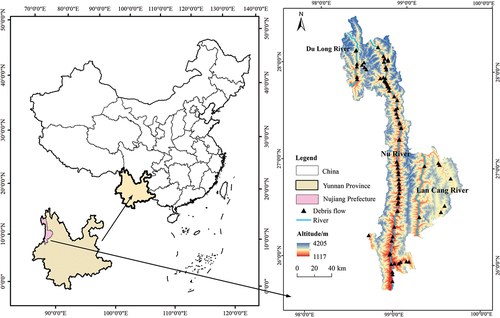
Nujiang Prefecture (25°33’~28°23’N, 98°09’~99°39’E) is located in southwest China, part of Yunnan Province. It has a total area of 14,703 square kilometers, with an average annual precipitation of 1,301.9 mm. The territory is densely populated by rivers, crisscrossing the country. The region is characterized by rugged terrain, with higher elevations in the north and lower elevations in the south, forming a typical high mountain and deep-cut canyon landscape. This geographical feature results from the juxtaposition of linear mountain ranges and longitudinal valleys within the area, as well as the geological characteristics of linear folding fractures and associated rock formations. Additionally, the region’s climate exhibits distinct wet and dry seasons, with the wet season significantly longer than the dry season. These factors collectively contribute to the high incidence of debris flow disasters in the area (Li et al., 2022). The geographic location and topographic distribution of Nujiang Prefecture are shown in Figure 1.

Figure 1. Overview map of the study area.

3. Materials and methods

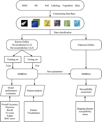
The method in this article consists of four main parts: 1. Establish the gully dataset and classify the gully according to its watershed area size, main gully length and elevation difference. 2. Construct the MMRNet model, evaluate its performance, and comparing it with other network models as well as machine learning methods. 3. Analyzing the feature extraction capabilities of the MMRNet model through feature visualisation. 4. Predict susceptibility based on the similarity between the gully to be evaluated and gullies where debris flows have occurred, and create a susceptibility assessment map for debris flows. The experimental workflow is shown in Figure 2.

Figure 2. Methodological flow chart of this study.

3.1. Materials used

The topographic and geomorphic features and material source conditions of the gully are prerequisites for debris flow formation (Cesca & D’Agostino, 2008). All gullies with certain topographic and geomorphic and material source conditions are at risk of debris flows, and rainfall is an external condition for debris flow formation.

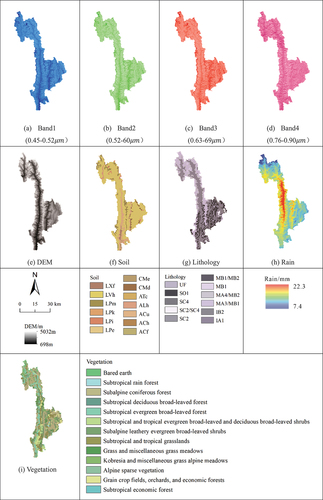
Digital elevation models, remote sensing images, lithology, soil, vegetation, and rainfall were chosen as the data sources for this research. The DEM can provide topographic information about the gully, such as gully area, gully length, slope, catchment area, and topographic elevation difference (Maerker et al., 2015). Remote sensing imagery can accurately depict the geomorphological characteristics of the gully, including vegetation cover, scour marks, and additional features. The data sources are shown in Table 1.

Table 1. Data sources.

Data	Source	Resolution
DEM	SRTM (https://srtm.csi.cgiar.org/)	30m
Remote sensing	https://data.cresda.cn/	16m
Lithology and soil	ISIRC (https://data.isric.org/)	90m
Vegetation	http://www.ncdc.ac.cn/	90m
Rain	NESDC (http://www.geodata.cn/)	1km

The process of selecting the positive sample is as follows. First, we consulted the Yunnan Disaster Reduction Guide, searched for news and literature on debris flow disasters in Yunnan Province. Then, the specific villages and gullies where debris flows occurred were identified by documented information combined with Google Earth. Images of gullies where debris flows have occurred were used as positive samples. Similarly the presence of villages in the vicinity of the gully and the absence of debris flows in the historical records. And images of gullies without visible scour marks and alluvial fans were categorised as negative samples. Finally, 286 positive samples, and 312 negative samples were identified within Yunnan Province, and a total of 672 gully samples were extracted within Nujiang Prefecture. The 672 gully samples contained 82 positive samples, 85 negative samples and 505 unknown gully samples. The 598 identified positive and negative samples were used for model training and testing, and the remaining 505 unknown gully samples were used for debris flow susceptibility assessment. The data were pixel-filled and standardised into images of 1280 pixels × 1280 pixels size, and the sample images are shown in Figure 3.

Figure 3. Experimental data.

Several studies have shown that the occurrence of debris flows is closely related to the watershed area and elevation difference of the gully (Banihabib et al., 2020; Yang et al., 2011). In order to more rationally distinguish the characteristic differences in debris flow susceptibility of gullies with different morphologies, while avoiding subjectivity in classification. On the basis of the positive and negative samples, we selected the watershed area size, the length of the main gully, and the elevation difference of the gully as indicators, used the K-means clustering method to divide each of the positive and negative samples into three categories. Where 0, 1, 2 are positive samples, 3, 4, 5 are negative samples, the number of each sample is shown in Table 2.

Table 2. Number of samples.

Category	Class	Number	Length/km	Elevation difference/km	Area/km^2
Positive	0	153	(2.3,15.4)	(1.1,2.9)	(1.0,24.0)
(occurred)	1	88	(9.8,18.8)	(1.5,3.2)	(26.0,64.0)
	2	45	(18.0,27.0)	(2.5,3.1)	(69.0,95.1)
Negative	3	126	(2.3,7.1)	(0.3,2.4)	(1.0,7.4)
(not	4	116	(4.9,15.6)	(0.7,2.9)	(7.5,19.2)
occurred)	5	70	(9.1,16.9)	(1.3,3.2)	(21.7,46.0)

3.2. Preview of convolutional neural network

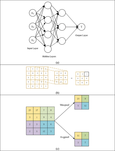
The convolutional neural network, as shown in Figure 4, consists of three components: input layer, hidden layer, and output layer. The hidden layer, also known as the middle layer, contains the convolutional layer, pooling layer, nonlinear activation layer, and fully connected layer. The convolutional layer is the most basic and important part of the convolutional neural network. The form of sliding is used to multiply the convolution kernel weights with different matrices of the image to get the input values of the next layer. Sequentially layer by layer different convolution kernels are used to extract the features of the image. Pooling layer, also known as downsampling layer, pooling layer directly takes the maximum or average value within the pooling range to reduce the data latitude of the feature map. No additional weight parameters are needed, reducing the amount of computation of downsampling and avoiding network overfitting to some extent. The fully connected layer is generally located at the end of the entire convolutional neural network. It is responsible for combining the two-dimensional features of the convolutional output and transforming them into a one-dimensional vector, thus realising the end-to-end learning process.

Figure 4. CNN model.

3.3. MMRNET

Debris flow dataset, with various features exhibiting different levels of richness. For instance, DEM (Digital Elevation Model) and remote sensing data encompass more diverse terrain and landform features, necessitating the use of deeper networks for training. On the other hand, sedimentary conditions and rainfall data contain relatively singular features, thus requiring simpler networks for training. Traditional convolutional neural network models have not adequately integrated multiple data sources, resulting in subpar identification performance. Therefore, inspired by existing model structures, this paper proposes a model called Multi-Modal Fusion Network (MMRNet) tailored for integrating diverse data sources related to mudslides. This model excels in effectively merging multiple data sources to provide a reasoned assessment of mudslide susceptibility.

The overall structure of the MMRNet proposed in this paper is shown in Figure 5. The MMRNet has two main parts, feature extraction and feature fusion. The feature extraction part uses a multi-scale feature fusion module to obtain more terrain and geomorphology features from DEM and remote sensing images, avoiding the problem of insufficient feature information extracted by a single feature scale. The feature information contained in the source conditions and rainfall data is relatively single, so the multi-scale feature fusion module was not used to avoid the redundancy of the extracted feature information. Furthermore, the use of the improved residual structure implemented feature reuse, reducing feature loss. By applying max-pooling to compress features, it substantially reduced the number of parameters, leading to improved evaluation efficiency. The feature fusion part, borrowed from ShuffleNet, uses a channel rearrangement technique to strengthen the correlation between each underlying feature. And the new features after channel rearrangement are feature extracted using an improved residual structure. The model finally outputs the similarity of the unknown gullies to the known gullies in each category through fully connected for susceptibility assessment. The loss function used is the Fusion Loss, which combines the Cross-Entropy Loss and the Focal Loss. It aims to achieve stability while increasing the feature differences between samples, enabling the network to pay more attention to the easily confused samples.

Figure 5. MMRNET model.

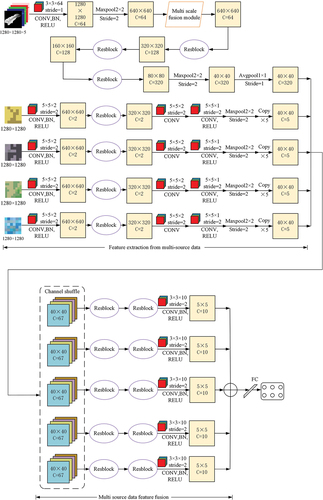
In the Figure 5: CONV stands for convolutional layer. C is the number of channels output from the convolutional layer. Stride is the step size. BN stands for batch normalisation. RELU stands for the activation function. Maxpool stands for the maximum pooling layer. Avgpool is the average pooling. FC is the fully connected layer.

3.3.1. Multi-scale feature fusion

In the debris flow gully image recognition task, spatial information is very important to extract gully features. Between gullies, there is a wide variety of terrain and topography. For instance, the features such as area, elevation difference, slope, and vegetation coverage among gullies exhibit variations. Describing the overall characteristics of gullies comprehensively using a single scale feature is challenging. A multi-scale feature set can address this issue, is shown in Figure 6. The multi-scale feature fusion module consists of three branches. The first branch, ‘Branch 1’, takes the original feature $S$ from the input module without any processing, serving as multi-scale feature 1. It retains the shallow feature information from the previous network layer. The second branch, ‘Branch 2’, processes the input features through a 3 × 3 convolutional layer. This branch uses a small-scale convolutional layer to capture local information within the gully, and the output feature is denoted as $F_{3\times 3}\left(S\right)$, representing multi-scale feature 2. The third branch, ‘Branch 3’, processes the input features through three 7 × 7 convolutional layers. This branch utilises larger-scale convolutional layers to capture deep and overall gully feature information. The output feature $F_{7\times 7}\left(F_{7\times 7}\left(F_{7\times 7}\left(S\right)\right)\right)$ is multi-scale feature 3. Subsequently, the features 1, 2, and 3 are element-wise added to obtain the new output feature. The fused feature can be represented as:

(1) $X=S+F_{3\times 3}\left(S\right)+F_{7\times 7}\left(F_{7\times 7}\left(F_{7\times 7}\left(S\right)\right)\right)$(1)

Figure 6. Multi scale feature fusion module.

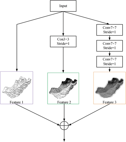
The fused feature X combines shallow, intermediate, and deep features from different scales. Compared to single-scale features, multi-scale fused features make more comprehensive use of both global and local features, incorporating a richer set of information. This approach helps to overcome issues associated with insufficient feature information in single-scale feature extraction.

3.3.2. Improved residual structure

As network depth increases, overfitting becomes a common issue. To address this, the paper introduces an improved residual structure, which enhances efficiency while reducing feature loss. In 2015, He and his colleagues introduced Residual Networks (Resnet) (He et al., 2016), which incorporated identity mappings, merging output features from higher and lower network layers. This improved feature reuse and, to some extent, preserved data integrity, addressing the information loss problem that traditional convolutional networks face during information transmission. It also mitigated issues such as gradient vanishing and exploding that can occur as network depth increases. The improved residual structure is illustrated in the Figure 7.

Figure 7. Residual structure.Where x is the input feature, F(x) is the residual mapping, and Y is the output result.

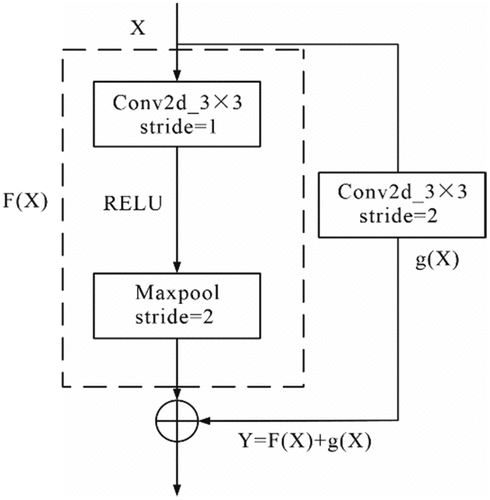
The improved residual structure adds a convolutional layer with a stride of 2 and a 3 × 3 kernel size, which reduces the size of the input feature X. This adjustment ensures that the output feature g(x) has the same size as the mapped feature F(x). Compared to feature F(x), g(x) undergoes fewer non-linear mappings, incorporating more shallow-layer features. In contrast to traditional residual structures, the improved residual structure not only merges features from the upper and lower network layers but also compresses the features, simplifying network complexity and significantly reducing the number of network parameters. This helps to better avoid overfitting issues, especially when dealing with limited debris flow gully data.

3.3.3. Channel rearrangement and feature fusion

Because the potential danger of gullies is a composite result of multiple factors, the feature fusion section primarily focuses on how to make full use of the extracted lower-level features and explore the correlations between different types of features. In a CNN, channels refer to the input and output of convolutional kernels, with the output channels containing the extracted features. Before performing feature fusion, channel rearrangement from ShuffleNet (Zhang et al., 2018) is used to reassemble the low-level features of different data types. This enhances the flow of various information, allowing the model to better learn the relationships between different types of features in subsequent fusion modules. In the specific implementation, the basic features extracted from the five classes are evenly divided into five portions, and one portion is taken from each class. These portions are then concatenated to create five combined datasets, each containing the low-level features from different classes. The diagram for channel rearrangement is shown in the Figure 8.

Figure 8. Channel rearrangement.

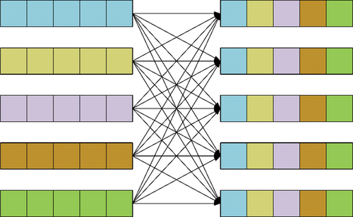
After channel rearrangement, in order to fuse these features as effectively as possible, an improved residual structure is employed for feature extraction. The features from each layer are continuously accumulated into the subsequent layers, merging shallow features with deep features to make full use of information from all layers. Finally, the five features output by the convolutional layers are element-wise added together to create a fused new feature.

3.3.4. Fusion loss function

The design purpose of MMRNet is to provide a reasonable susceptibility assessment for gullies of different shapes. Therefore, when training the network for gully classification tasks, it is required that the model can distinguish the morphological differences between different categories of gullies and also differentiate the feature differences between positive and negative samples. CNN parameters are optimised through backpropagation, and the loss function plays a crucial role in controlling the direction and process of optimisation.

For the problem of distinguishing morphological features of gullies, the more stable Cross Entropy (CE) is used. In this paper, gullies are divided into 6 classes. Let $p$ denote the output of MMRNet, and $p_i\left(i=0,\cdots ,5\right)$ denotes the feature similarity between the input gullies and the gullies of the i-th class. When the gully belongs to class i, $y_i=1$, otherwise, $y_i=0$. The gully multi-class cross-entropy loss can then be represented as:

(2) $C_E\left(P\right)=-{\displaystyle \sum _{i=0}^5{y}_i}\log \left(p_i\right)$(2)

For the distinction between positive and negative sample features, refer to the design idea of Focus Loss Function (Lin et al., 2017): the weight factor is used to reinforce the loss of fewer or harder samples, forcing the network to pay more attention to such sample features. We propose a loss function Fusion Loss that reinforces the difference between positive and negative sample features of the gully, which is of the form:

(3) $F_L\left(p_i\right)=-\alpha \log \left({\displaystyle \sum _{i=0}^2{p}_i}\right)ifl\in \left\{0,1,2\right\}-\alpha \log \left({\displaystyle \sum _{i=3}^5{p}_i}\right)ifl\in \left\{3,4,5\right\}\text{.}$(3)

In the equation: $\alpha$ is the penalty coefficient, an adjustable hyperparameter, the larger the value indicates that more importance is attached to the differences between positive and negative samples. Through experiments it is found that the model works best when $\alpha =2$, $l\in \left\{0,1,2,3,4,5\right\}$ is the true category of gullies. Assuming that the sample is a disaster-prone gully, then its $l\in \left\{0,1,2\right\}$. If at this point the model output trench is more similar to the positive sample 0, 1, 2 class features, it can be seen that ${\sum }_{i=0}^2{p}_i\to 1$, i.e. $log\left({\sum }_{i=0}^2{p}_i\right)\to 0$, then there will be almost no loss. If at this point the model outputs that the gully is more similar to the negative sample 3,4,5 classes, it can be seen that ${\sum }_{i=0}^2{p}_i\to 0$, $-\alpha log\left({\sum }_{i=0}^2{p}_i\right)\to +\mathrm{\infty }$, i.e. the FL imposes a large penalty on this determination.

In summary, in order to synthesise the characteristic differences between the gullies of each form and between the positive and negative samples, the final loss function selected in this study is:

(4) $Loss=C_E\left(P\right)+F_L\left(P\right)$(4)

4. Experimental results and analysis

4.1. Experimental environment and evaluation indicators

The hardware implemented in this experiment is: Intel Xeon E5–2686 v4, hard disk 200 G, memory 60 G, GPU: NVIDIA RTX A4000, graphics card memory 16 G. Software environment: Ubuntu18.04, python3.8, PyTorch1.11, Cuda11.3. The experiments set the Batch size to 4, the optimisation method is gradient descent (SGD), the learning rate is set to 0.0001, and a total of 50 rounds of training.

The assessment indexes in this paper contain Overall Accuracy, Precision, Recall, F1-score and Kappa factor. Overall Accuracy is calculated as:

(5) $OA=\frac{T_P+T_N}{T_P+F_N+T_N+F_P}$(5)

Where $T_P$ denotes the number of positive samples predicted to be positive, $F_N$ denotes the number of positive samples predicted to be negative, $T_N$ denotes the number of negative samples predicted to be negative, and $F_P$ denotes the number of negative samples predicted to be positive.

Using $T_P$ and $F_P$ can represent the Precision rate, which is calculated by the formula:

(6) $P_{recision}=\frac{T_P}{T_P+F_P}$(6)

Recall is the proportion of positive samples that are predicted to be positive:

(7) $R_{ecall}=\frac{T_P}{T_P+F_N}\hspace{0.17em}$(7)

The F1-score is used to measure the classification accuracy and is calculated by the following formula:

(8) $F_1=2\times \frac{P_{recision}\times R_{ecall}}{P_{recision}+R_{ecall}}$(8)

Kappa coefficient is used to measure the classification accuracy and is calculated by the following formula:

(9) $K_{appa}=\frac{p_0-p_e}{1-p_e}$(9)

Where $p_0$ is the overall classification accuracy, which is calculated by dividing the sum of the number of correctly classified samples in each category by the total number of samples, using the following formula:

(10) $p_0=\frac{T_P+T_N}{T_P+F_N+T_N+F_P}\left(10\right)$(10)

${\mathrm{p}}_{\mathrm{e}}$ is the chance consistency error or expected consistency rate, as calculated in the following equation:

$p_e=\frac{\left(T_P+F_P\right)\times \left(T_P+F_N\right)+\left(F_P+T_N\right)\times \left(F_N+T_N\right)}{{\left(T_P+F_N+T_N+F_P\right)}^2}\hspace{0.17em}\left(11\right)$

4.2. Model performance evaluation

In order to test the MMRNet model’s ability to predict the potential dangerousness of debris flows, the common deep learning networks VGG16 (Simonyan et al., 2014), ResNet18, ResNet34, ShuffleNet, DenseNet-121 (Huang et al., 2017), ResNext (Xie et al., 2017), MobileNet (Howard Andrew et al., 2017), and InceptionVI (Szegedy et al., 2017) are selected as comparison objects. Meanwhile, a comparison was made with the neural network model DRSNet from the literature (Xu & Wang, 2022). In order to make a comparison with the method of statistical factors, 11 influence factors, namely area, length of main ditch, elevation difference, curvature, slope, SPI, NDVI, soil, lithology, and rainfall, were selected according to the method of literature (Gu et al., 2023). These factors are used in BP neural network, SVM, and Random Forest(RF) for classification. The results of the comparison test are shown in Table 3. As can be seen from Table 3, the prediction performance of the MMRNet model is more satisfactory, with an accuracy of 81.6%, which is obviously better than other models. It can identify the debris flow gullies better. Even in the case of a small number of samples, it can also achieve good prediction results, which shows that the model has good generalisation ability.

Table 3. Classification performance comparison.

Model	OA/%	P/%	R/%	F1	Kappa
MMRNet	81.6	81.9	82.4	0.841	0.78
VGG16	71.7	76.4	72.3	0.743	0.68
ResNet18	74.7	76.8	74.8	0.758	0.71
ResNet34	72.7	72.8	77.1	0.749	0.67
ShuffleNet	72.9	73.3	74.5	0.739	0.68
DenseNet	76.2	75.7	76.6	0.761	0.72
ResNext	75.0	76.4	77.2	0.768	0.70
MobileNet	70.3	75.1	69.5	0.722	0.69
InceptionVI	73.3	72.9	75.0	0.739	0.68
DRSNet	78.5	80.2	83.9	0.811	0.749
SVM	73.1	67.1	75.3	0.710	0.70
BP	71.9	73.3	67.1	0.701	0.67
RF	74.6	68.3	78.8	0.732	0.71

In order to further effectively evaluate the prediction ability of MMRNet for the susceptibility of debris flow, this paper uses the Receiver Operating Characteristic (ROC) curve to evaluate the model performance, as shown in Figure 9. The results show that the AUC value of MMRNet is 0.8320, indicating that MMRNet can predict the susceptibility of debris flow better.

Figure 9. ROC curve.

4.3. Analysis of feature extraction capability of each improved module

In order to explore the role of different modules in the network for feature extraction of debris flow gullies, this section conducted the following ablation experiments to compare the improved MMRNet with the original network framework, and the experimental results are shown in the Table 4. From the results, it can be seen that the improved residual structure makes the accuracy of the original network increase by 3.4%, which is a more obvious improvement. The introduction of Fusion Loss improves the classification accuracy of the network, but the magnitude is smaller. By comparing the results of the five experiments, it can be concluded that when the multi-scale feature fusion module, improved residual structure, channel rearrangement, and Fusion Loss are used together, the network achieves the highest classification accuracy. Compared to the original network, this approach resulted in an 8.3% increase in accuracy.

Table 4. Ablation experiment.

Multi-scale feature fusion module	Improved residual structure	Channel rearrangement	Fusion Loss	Accuracy(%)
×	×	×	×	73.3
√	×	×	×	75.9
√	√	×	×	79.3
√	√	√	×	80.5
√	√	√	√	81.6

In order to reflect more intuitively the specific effects of multi-scale feature fusion and improved residual structure on the feature extraction of debris flow gullies, two sets of ablation experiments are conducted here to visualise the feature maps output from different structures. The experimental results are shown in Figure 10.

Figure 10. Comparison of feature maps.

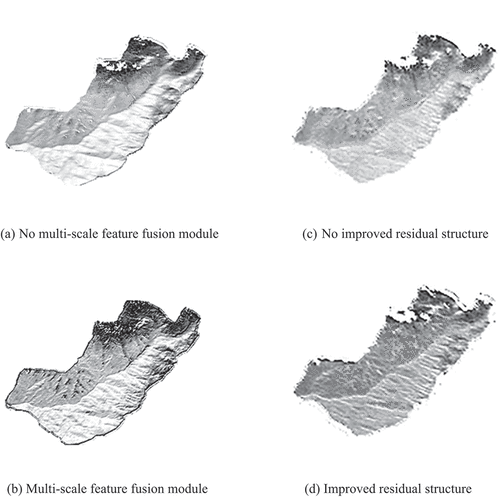
Comparing Figure (a) and Figure (b), it can be observed that in the network without the multi-scale feature fusion module, the output feature maps lack detail, such as missing vegetation cover and erosion traces in local features, and there is a loss in overall features. Adding the multi-scale feature fusion module results in feature maps that better represent both the local and overall features of debris flow gullies. Therefore, introducing the multi-scale feature fusion module can provide a better representation of both global and local features in debris flow gully images.

Comparing Figure (c) and Figure (d), it can be seen that the feature maps from the network without the improved residual structure suffer from severe information loss. Introducing the improved residual structure results in more complete feature maps, indicating that it allows the network to better integrate shallow and deep features, leading to more complete feature extraction and reducing feature loss.

4.4. Analysis of the feature extraction capability of the overall model

In order to further analyse the model’s ability to extract image features, the feature maps extracted by the model are visualised and compared with the factors extracted by ArcGIS, as shown in Figure 11.

Figure 11. Analysis of gully characteristic map.

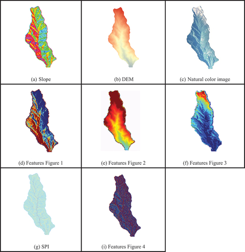
Figure (d), Figure (e), Figure (f), Figure (i) show the topographic and geomorphic features extracted from debris flow gully images by MMRNet. Figure (a) is the slope orientation map of the gully extracted from the DEM by ArcGIS, the slope orientation mainly controls the degree of solar radiation leading to temperature, evaporation, vegetation, rock weathering, etc. Comparing Figure (a) and Figure (d), it can be seen that the Figure (d) can better respond to the information of slope orientation of the gully, so it can be obtained the slope orientation features of the gully by MMRNet.

Figure (b) displays the DEM of the gully, which provides an intuitive representation of the gully’s topographical elevation differences. Changes in elevation primarily impact the distribution of precipitation and vegetation. In Figure (e), areas with deeper colours indicate higher elevations in the gully, which is generally consistent with the information in Figure (b). Therefore, MMRNet can effectively capture the topographical features of the gully.

Vegetation plays a role in water conservation and helps prevent soil erosion and desertification. Figure (c) represents a synthesised natural colour image of the gully obtained from remote sensing data. It provides an intuitive depiction of the gully’s vegetation coverage and erosion traces. By rendering the feature maps output by MMRNet into a heatmap, Figure (f) is obtained. In this heatmap, areas with higher vegetation coverage have cooler tones, while areas with less vegetation cover and erosion traces have warmer tones. Figure (f) offers a visual representation of the gully’s vegetation coverage, indicating that MMRNet effectively extracts the topographical features of the gully.

SPI stands for Stream Power Index, which is used to measure the erosive power of water flow. A higher SPI value indicates that concentrated runoff may lead to soil erosion and increase the likelihood of debris flows. Figure (g) shows the SPI map of the gully extracted from ArcGIS. Comparing Figure (g) and Figure (i), it can be observed that MMRNet can extract similar features.

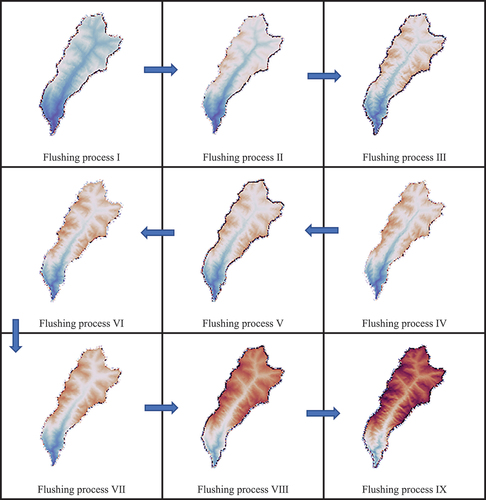
In addition to capturing the topographical features of the gully, convolutional neural networks can also extract information about the erosion process of debris flows. Different stages of the debris flow erosion process are represented by multiple feature maps extracted from the DEM by the neural network. As shown in Figure 12, water converges at the head of the gully, carries sediment downstream along the terrain, and eventually discharges at the gully mouth.

Figure 12. Debris flow flushing process.

4.5. Assessment results and analysis of debris flow susceptibility in gullies and valleys of Nujiang Prefecture

First the parameters of the network model with the highest accuracy in the test set were saved. The parameters were read, and 672 gully samples were fed into the network, outputting the probability that each gully was predicted to be a positive sample. Secondly, the output probabilities were categorised into five intervals corresponding to five levels of susceptibility using the natural breakpoint method: very low susceptibility zone [0, 0.0813], low susceptibility zone [0.0813, 0.2512], medium susceptibility zone [0.2512, 0.5232], high susceptibility zone [0.5232, 0.8296], and very high susceptibility zone [0.8296, 1]. Finally, the gully DEM was imported into ArcGIS to visualise the susceptibility zoning, and the susceptibility zoning results are shown in Figure 13:

Figure 13. Debris flow susceptibility map for Nujiang Prefecture.

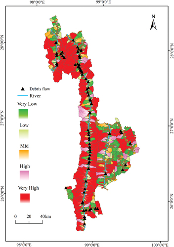
From the results of debris flow susceptibility zoning obtained from the MMRNet model, it can be seen that: the distribution of high and very high susceptibility zones and low and very low susceptibility zones is more concentrated. The high susceptibility and extremely high susceptibility zones are primarily concentrated on both sides of the river, indicating that the river system plays a significant role in promoting the formation of debris flows. This results in debris flows in Nujiang Prefecture being more concentrated along the riverbanks. The low susceptibility zones and the very low susceptibility zones are mainly concentrated and distributed in the eastern part of Nujiang Prefecture, with a small amount in the northern part of Nujiang Prefecture.

Debris flow density is the ratio of the proportion of historical disaster gullies within a susceptible area to the proportion of the area of that susceptible zone. It provides a relatively intuitive reflection of the intensity of debris flows within the susceptibility zone. In the model’s susceptibility gully zoning results, as shown in Table 5, the debris flow density for the extremely high susceptibility zone is 1.60, indicating that the assessment results are quite reasonable.

Table 5. Susceptibility classification and debris flow density in Nujiang Prefecture.

Level	Area（$k{m}^2$）	Area ratio (%)	Number of gullies	Number of historical disaster gullies	Percentage of historical disaster gullies (%)	Density of debris flows
Very Low	2273.80	17.68	302	1	1.22	0.07
Low	689.29	5.36	80	0	0	0
Mid	722.33	5.62	51	0	0	0
High	1242.27	9.66	60	0	0	0
Very High	7931.00	61.68	179	81	98.78	1.60
Total	12858.69		672	82	100.00

In order to assess the effect of each factor on debris flow susceptibility, the common area, elevation difference, slope, NDVI, and SPI factors are selected here for visualisation, as shown in Figure 14.

Figure 14. Distribution of gully area, elevation difference, normalized difference vegetation index (NDVI), and stream power index (SPI) in the susceptibility zones.

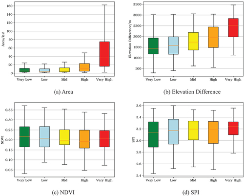
From the Figure 14, it can be observed that area, elevation difference, stream power index(SPI), and debris flow susceptibility level are positively correlated. As the average values of area, elevation difference, and SPI increase, the debris flow susceptibility level also shows an upward trend. Larger gullies with extensive areas are conducive to rainwater collection, and they have sufficient solid material sources. Elevation difference provides potential energy for the formation of debris flows. The strong erosion of loose deposits by water flow is a necessary condition for debris flow formation, and a higher SPI indicates stronger erosion of loose deposits. Therefore, gullies with larger areas, greater elevation differences, and higher SPI values tend to have higher susceptibility to debris flows.

Normalized difference vegetation index (NDVI) is negatively correlated with debris flow susceptibility levels. As the average values of the NDVI increase, the debris flow susceptibility levels tend to decrease. A higher NDVI is favourable for water conservation and helps prevent soil erosion.

5. Discussion

Our research has established a Multi-Channel Multi-Scale Residual Network (MMRNet) capable of extracting characteristics of gullies prone to debris flows. This model effectively integrates multiple data sources and objectively, efficiently, and accurately assesses the susceptibility to debris flows, producing susceptibility zone maps for the Nujiang Prefecture. From the susceptibility zone map, it can be observed that gullies identified as extremely high susceptibility are distributed along both sides of the river. This implies that water erosion plays a facilitating role in the formation of debris flows.

Compared to on-site inspection methods (Lyu et al., 2022), this approach can save a significant amount of manpower and resources, allowing for the remote assessment of the susceptibility to debris flows over large areas. However, when conditions permit, combining it with on-site inspections can make the assessment results more reasonable. Compared to physical modelling methods (Baum et al., 2010), this approach can assess the susceptibility of several hundred gullies in one go, making it more suitable for tasks involving the assessment of susceptibility over large areas. Compared to statistical and traditional machine learning methods, this approach reduces human intervention, avoiding subjectivity in the selection of influencing factors during susceptibility assessment. And, it references the method by Gu et al., selecting 11 influencing factors, comparing this with the method of manually selecting influencing factors. We selected the BP neural network, SVM, and RF models to classify debris flow gullies. The results indicate that MMRNet outperforms traditional machine learning models in the recognition of debris flow gullies. In comparison to the DRSNet method used by Xu, this study takes into consideration that CNNs require a rich dataset to better extract gully features and, therefore, integrates multiple data sources to construct a more comprehensive dataset. Through controlled experiments, MMRNet demonstrates stronger recognition performance for debris flow gullies, with all evaluation metrics surpassing those of DRSNet. As a result, it provides a more reasonable assessment of debris flow susceptibility.

At the same time, this study still has some limitations. It is constrained by a limited sample size and relatively low data resolution. Subsequent research will focus on addressing these issues to achieve better assessment results.

6. Conclusion

This study, conducted in the Nujiang Prefecture, integrated multiple data sources, including DEM, remote sensing imagery, soil, lithology, vegetation, and rainfall data. It introduced MMRNet to extract topographical features, source conditions, and rainfall information related to debris flow gullies. In the model construction, several structures, such as multi-scale feature modules, improved residual structures, and channel rearrangement, were used to enhance the extraction of features from gully images.

Using MMRNet, a comprehensive and objective assessment of debris flow susceptibility was carried out for all gullies within the Nujiang Prefecture. The experimental results demonstrate that:

1. Through experiments, MMRNet achieved an accuracy of 81.6% in the six-class classification of gully images, with an AUC value of 0.8320. In susceptibility zones, as the susceptibility level increases, the debris flow density also gradually increases, indicating that using convolutional neural networks for debris flow susceptibility assessment is feasible and effective.

2. The visualisation of MMRNet meso-level features shows that the model is able to extract key features of debris flow causation such as elevation difference, vegetation cover, slope direction, SPI, etc., and even capture the scouring process of the debris flow.

3. From the results of the susceptibility zoning, it can be seen that the extremely high and high susceptibility areas of debris flows are mostly distributed in the places with abundant water systems on both sides of the river, implying that the water systems have a greater contribution to the formation of debris flows.

The main contribution of this paper is the introduction of MMRNet, a Convolutional Neural Network specifically designed for large-scale debris flow susceptibility assessment. This model excels in the fusion of multi-source data, automating the extraction of topographical features and source conditions within gullies, thereby reducing the need for manual intervention. It offers an objective, efficient, and accurate assessment of debris flow susceptibility for all gullies within the Nujiang Prefecture. This approach provides new insights for remote, large-scale debris flow prevention and management in the future. With the expansion of the dataset and the improvement in the performance of deep learning models, the evaluation results are expected to become increasingly reasonable.

Disclosure statement

No potential conflict of interest was reported by the author(s).

Data availability statement

DEM can be downloaded from SRTM (https://srtm.csi.cgiar.org/). Remote sensing can be downloaded from https://data.cresda.cn/. The data of lithology, soil can be downloaded from ISIRC (https://data.isric.org/). Vegetation can be downloaded from http://www.ncdc.ac.cn/. The rainfall data can be downloaded from NESDC (http://www.geodata.cn/). The data that support the findings of this study are available from the corresponding author, Dr. Baoyun Wang, upon reasonable request.

Additional information

Funding

This work was supported by the National Natural Science Foundation of China(grant number 61966040)

References

- Banihabib, M. E., Tanhapour, M., & Roozbahani, A. (2020). Bayesian networks model for identification of the effective variables in the forecasting of debris flows occurrence. Environmental Earth Sciences, 79(8), 1–15. https://doi.org/10.1007/s12665-020-08911-w
- Baum, R. L., Godt, J. W., & Savage, W. Z. (2010). Estimating the timing and location of shallow rainfall‐induced landslides using a model for transient, unsaturated infiltration. Journal of Geophysical Research: Earth Surface, 115(F3), 115. https://doi.org/10.1029/2009jf001321
- Bonasera, M., Cerrone, C., Caso, F., Lanza, S., Fubelli, G., & Randazzo, G. (2022). Geomorphological and structural assessment of the coastal area of capo faro promontory, NE Salina (Aeolian Islands, Italy)’. Land, 11(7), 1106. https://doi.org/10.3390/land11071106
- Cesca, M., & D’Agostino, V. (2008). Comparison between FLO-2D and RAMMS in debris-flow modelling: A case study in the dolomites. WIT Transactions on Engineering Sciences, 60, 197–206. https://doi.org/10.2495/DEB080201
- Chang, T.-C., & Chao, R.-J. (2006). Application of back-propagation networks in debris flow prediction. Engineering Geology, 85(3–4), 270–280. https://doi.org/10.1016/j.enggeo.2006.02.007
- Chang, M., Tang, C., Zhang, D.-D., & Guo-Chao, M. (2014). Debris flow susceptibility assessment using a probabilistic approach: A case study in the Longchi area, Sichuan province, China. Journal of Mountain Science, 11(4), 1001–14. https://doi.org/10.1007/s11629-013-2747-9
- Chen, Y., Qin, S., Qiao, S., Dou, Q., Che, W., Gang, S., Yao, J., & Emmanuel Nnanwuba, U. (2020). Spatial predictions of debris flow susceptibility mapping using convolutional neural networks in Jilin Province, China. Water, 12(8), 2079. https://doi.org/10.3390/w12082079
- Choi, S.-K., & Kwon, T.-H. (2021). A case study on the closed-type barrier effect on debris flows at mt. Woomyeon, Korea in 2011 via a numerical approach. Energies, 14(23), 7890. https://doi.org/10.3390/en14237890
- Dash, R. K., Omowumi Falae, P., & Prasanna Kanungo, D. (2022). Debris flow susceptibility zonation using statistical models in parts of Northwest Indian Himalayas—implementation, validation, and comparative evaluation. Natural Hazards, 111(2), 2011–2058. https://doi.org/10.1007/s11069-021-05128-3
- Gomes, R., Guimarães, R., de Carvalho, J. O., Fernandes, N., & Do Amaral Júnior, E. (2013). Combining spatial models for shallow landslides and debris-flows prediction. Remote Sensing, 5(5), 2219–37. https://doi.org/10.3390/rs5052219
- Gu, F., Chen, J., Sun, X., Yongchao, L., Zhang, Y., & Wang, Q. (2023). Comparison of machine learning and traditional statistical methods in debris flow susceptibility assessment: A case study of Changping District, Beijing. Water, 15(4), 705. https://doi.org/10.3390/w15040705
- Hakim, W. L., Rezaie, F., Nur, A. S., Panahi, M., Khosravi, K., Lee, C. W., & Lee, S. (2022). Convolutional neural network (CNN) with metaheuristic optimization algorithms for landslide susceptibility mapping in Icheon, South Korea. Journal of Environmental Management, 305, 114367. https://doi.org/10.1016/j.jenvman.2021.114367
- He, K., Zhang, X., Ren, S., & Sun, J. 2016. Deep residual learning for image recognition. In Proceedings of the IEEE conference on computer vision and pattern recognition, 770–78. https://doi.org/10.48550/arXiv.1512.03385
- Howard Andrew, G., Menglong, Z., Bo, C., Dmitry, K., Weijun, W., Tobias, W., Marco, A., & Hartwig, A. (2017). Mobilenets: Efficient convolutional neural networks for mobile vision applications. In Proceedings of the IEEE conference on computer vision and pattern recognition. https://doi.org/10.48550/arXiv.1704.04861
- Hsu, Y.-C., & Liu, K.-F. (2019). Combining TRIGRS and DEBRIS-2D models for the simulation of a rainfall infiltration induced shallow landslide and subsequent debris flow. Water, 11(5), 890. https://doi.org/10.3390/w11050890
- Huang, G., Liu, Z., Van Der Maaten, L., & Weinberger, K. Q. 2017. Densely connected convolutional networks. In Proceedings of the IEEE conference on computer vision and pattern recognition, 4700–08. https://doi.org/10.48550/arXiv.1608.06993
- Jakob, M., Hungr, O., & Matthias Jakob, D. (2005). Debris-flow Hazards and related phenomena. Springer). https://doi.org/10.1007/b138657
- Kim, M., Lee, S., Kwon, T.-H., Choi, S.-K., & Jeon, J.-S. (2021). Sensitivity analysis of influencing parameters on slit-type barrier performance against debris flow using 3D-based numerical approach. International Journal of Sediment Research, 36(1), 50–62. https://doi.org/10.1016/j.ijsrc.2020.04.005
- Lauro, C., Moreiras, S. M., Junquera, S., Vergara, I., Toural, R., Wolf, J., & Tutzer, R. (2017). Summer rainstorm associated with a debris flow in the Amarilla gully affecting the international Agua Negra Pass (30°20′S), Argentina. Environmental Earth Sciences, 76(5), 1–12. https://doi.org/10.1007/s12665-017-6530-z
- Li, Z., Chen, J., Tan, C., Zhou, X., Yuchao, L., & Han, M. (2021). Debris flow susceptibility assessment based on topo-hydrological factors at different unit scales: A case study of Mentougou district, Beijing. Environmental Earth Sciences, 80(9), 1–19. https://doi.org/10.1007/s12665-021-09665-9
- Li, Y., Deng, X., Ji, P., Yang, Y., Jiang, W., & Zhao, Z. (2022). Evaluation of landslide susceptibility based on CF-SVM in Nujiang Prefecture. International Journal of Environmental Research and Public Health, 19(21), 14248. https://doi.org/10.3390/ijerph192114248
- Lin, T.-Y., Goyal, P., Girshick, R., Kaiming, H., & Dollár, P. 2017. Focal loss for dense object detection. In Proceedings of the IEEE international conference on computer vision, 2980–88. https://doi.org/10.48550/arXiv.1708.02002
- Lombardo, L. G., Fubelli, G., Amato, & Bonasera, M. (2016). Presence-only approach to assess landslide triggering-thickness susceptibility: A test for the Mili catchment (north-eastern Sicily, Italy)’. Natural Hazards, 84(1), 565–88. https://doi.org/10.1007/s11069-016-2443-5
- Lyu, L., Mengzhen, X., Wang, Z., Cui, Y., & Blanckaert, K. (2022). A field investigation on debris flows in the incised Tongde sedimentary basin on the northeastern edge of the Tibetan Plateau. Catena, 208, 105727. https://doi.org/10.1016/j.catena.2021.105727
- Maerker, M., Quénéhervé, G., Bachofer, F., & Mori, S. (2015). A simple DEM assessment procedure for gully system analysis in the Lake Manyara area, northern Tanzania. Natural Hazards, 79(S1), 235–253. https://doi.org/10.1007/s11069-015-1855-y
- Qiu, C., Su, L., Zou, Q., & Geng, X. (2022). A hybrid machine-learning model to map glacier-related debris flow susceptibility along Gyirong Zangbo watershed under the changing climate. The Science of the Total Environment, 818, 151752. https://doi.org/10.1016/j.scitotenv.2021.151752
- Rodríguez-Morata, C., Villacorta, S., Stoffel, M., & Antonio Ballesteros-Cánovas, J. (2019). Assessing strategies to mitigate debris-flow risk in Abancay province, south-central Peruvian Andes. Geomorphology, 342, 127–139. https://doi.org/10.1016/j.geomorph.2019.06.012
- Romeo, S., D’Angiò, D., Fraccica, A., Licata, V., Vitale, V., Chiessi, V., Amanti, M., & Bonasera, M. (2023). ‘Investigation and preliminary assessment of the Casamicciola landslide in the island of ischia (Italy) on November 26, 2022. Landslides, 20(6), 1265–76. https://doi.org/10.1007/s10346-023-02064-0
- Simoni, A., Bernard, M., Berti, M., Boreggio, M., Lanzoni, S., Maria Stancanelli, L., & Gregoretti, C. (2020). Runoff-generated debris flows: Observation of initiation conditions and erosion–deposition dynamics along the channel at Cancia (eastern Italian Alps). Earth Surface Processes and Landforms, 45(14), 3556–71. https://doi.org/10.1002/esp.4981
- Simonyan, K., Vedaldi, A., & Zisserman, A. (2014). Very deep convolutional networks for large-scale image recognition. In Proceedings of the IEEE conference on computer vision and pattern recognition, 36 (8). 1573–85. https://doi.org/10.48550/arXiv.1409.1556
- Szegedy, C., Ioffe, S., Vanhoucke, V., & Alemi, A. 2017. Inception-v4, inception-resnet and the impact of residual connections on learning. In Proceedings of the AAAI conference on artificial intelligence. https://doi.org/10.1609/aaai.v31i1.11231
- Takahashi, T. (2007). Debris flow. Taylor & Francis). https://doi.org/10.1201/9780203946282
- Tang, C., Zhu, J., Li, W. L., & Liang, J. T. (2009). Rainfall-triggered debris flows following the Wenchuan earthquake. Bulletin of Engineering Geology and the Environment, 68(2), 187–194. https://doi.org/10.1007/s10064-009-0201-6
- Wu, S., Chen, J., Zhou, W., Iqbal, J., & Yao, L. (2018). A modified Logit model for assessment and validation of debris-flow susceptibility. Bulletin of Engineering Geology and the Environment, 78(6), 4421–38. https://doi.org/10.1007/s10064-018-1412-5
- Xie, S., Girshick, R., Dollár, P., Zhuowen, T., & Kaiming, H. 2017. Aggregated residual transformations for deep neural networks. In Proceedings of the IEEE conference on computer vision and pattern recognition, 1492–500. https://doi.org/10.48550/arXiv.1611.05431
- Xu, F., & Wang, B. (2022). Debris flow susceptibility mapping in mountainous area based on multi-source data fusion and CNN model – taking Nujiang Prefecture, China as an example. International Journal of Digital Earth, 15(1), 1966–88. https://doi.org/10.1080/17538947.2022.2142304
- Yang, Q., Gao, J., Wang, Y., & Qian, B. (2011). Debris flow characteristics and risk degree assessment in Changyuan gully, Huairou District, Beijing. Procedia Earth and Planetary Science, 2, 262–271. https://doi.org/10.1016/j.proeps.2011.09.042
- Yao, T., Thompson, L., Yang, W., Wusheng, Y., Gao, Y., Guo, X., Yang, X., Duan, K., Zhao, H., Baiqing, X., Jiancheng, P., Anxin, L., Xiang, Y., Kattel, D. B., & Joswiak, D. (2012). Different glacier status with atmospheric circulations in Tibetan plateau and surroundings. Nature Climate Change, 2(9), 663–67. https://doi.org/10.1038/nclimate1580
- Zhang, Y., Taotao, G., Tian, W., & Liou, Y.-A. (2019). Debris flow susceptibility mapping using machine-learning techniques in Shigatse area, China. Remote Sensing, 11(23), 2801. https://doi.org/10.3390/rs11232801
- Zhang, X., Zhou, X., Lin, M., & Sun, J. 2018. Shufflenet: An extremely efficient convolutional neural network for mobile devices. In Proceedings of the IEEE conference on computer vision and pattern recognition, 6848–56. https://doi.org/10.48550/arXiv.1707.01083