Surrogate-based optimization for overflow spillway design

ABSTRACT

Overflow spillways are essential structures of dam projects, releasing surplus flood water to ensure dam safety. The discharge capacity of these structures depends mainly on their geometry; the most common shape is the standard weir, designed empirically. The design of overflow spillways must be optimised with respect to hydraulic performance, dam safety requirements and economic cost. The objective of this work is to numerically investigate spillway design using a shape optimisation process based on computational fluid dynamics software. The program Code_Saturne, which uses the volume of fluid method, was used to optimise the spillway design. To decrease computational cost, two reduced-order models were constructed. The first, with independent error formulation, was based on a neural network model, and the second was based on a kriging model, which considers correlated error formulation. The spillway optimisation was performed by a metaheuristic using each surrogate model as a simulator, and results are compared with those of the standard weir. The numerical optimisation results show an improvement over standard spillway hydraulic performances. Based on the optimised spillway shapes, expected gains are up to 15% for the flow discharge.

RESUME

Les évacuateurs de crue sont des dispositifs hydrauliques assurant la sureté des barrages. Ils sont conçus pour évacuer l’excédent de débit ne pouvant être stocké dans la retenue. Leurs capacités d’évacuation dépendent principalement de leurs formes géométriques. La forme la plus répandue du déversoir standard n’a été définie qu’empiriquement et optimiser la forme de ces ouvrages afin d’améliorer leurs performances présente des intérêts à la fois financiers et de sûreté. L’objectif de ce travail est d’étudier la conception d’évacuateur de crue par processus d’optimisation de forme basé sur un code de dynamique des fluides. La méthode de Code_Saturne a été utilisée pour optimiser la conception du déversoir afin d’augmenter la débitance du seuil déversant pour une hauteur d’eau donnée en amont. Afin de réduire les coûts de calcul, deux modèles réduits ont été construits. Le premier, avec une formulation d’erreurs indépendantes, est basé sur un modèle de réseau de neurones, tandis que le second, considérant une formulation d’erreurs corrélées, est basé sur la méthode de krigeage. L’optimisation est réalisée par une méta-heuristique qui prend comme simulateur chacun des modèles réduits. Les résultats montrent une amélioration des performances hydrauliques du déversoir standard. Les formes optimisées présentent des gains attendus de 15 % sur le débit.

KEYWORDS:

• Computational fluid dynamics (CFD)
• spillways design
• optimisation
• reduced-order models
• volume of fluid method (VOF)

MOTS-CLES:

• Calcul de dynamique des fluides (CFD)
• conception d’évacuateur de crue
• optimisation
• modèles réduits
• méthode « volume of fluid » (VOF)

1. Introduction

The global resurgence in demand for hydroelectricity requires the construction of several hundred dams each year and therefore almost as many spillways. In 2014, Zarfl et al. (2015) counted 3700 hydroelectric dams with a generating capacity of more than 1 MW either planned or being built. Available knowledge on the hydraulic process and design of overflow spillways relies generally on laboratory studies and, to a limited extent, on numerical modelling. Bazin (1898)’s studies are often cited as preliminary works in the design of straight-crested spillways. The first hydrodynamic geometries for spillways were proposed by Müller (1908) and Creager (1917). Further works on the trajectory of the flow overtopping the straight-crested weir were conducted by Scimemi (1937) and De Marchi (1928). However, there was no standardisation of spillway geometry prior to the United States Army, Corps of Engineers (USACE, 1977), based on Abecasis (1970)’s work. For more details on the design of straight-crest spillways and their performance, the reader may refer to Hager and Schleiss (2009) and Hager and Castro-Orgaz (2017).

To date, spillway shapes have been developed based on experimental studies. However, physical models suffer from scaling effects and are costly. On the other hand, computational fluid dynamics (CFD) provides a cost-effective method to simulate flow over spillways with accuracy. In fact, several numerical studies of flow over spillways were carried out to assess the accuracy of numerical models in comparison with experimental data (Dargahi, 2006; Imanian & Mohammadian, 2019). However, neither numerical nor experimental studies have been reported in the literature to explore new geometries and to optimise the shape of overflow spillways, even though there is a growing interest in enhancing their hydraulic performances. Recently, however, Hosseini et al. (2016) followed by Ferdowsi et al. (2019) presented a methodology to optimise labyrinth spillways’ shape. The former study minimised their construction cost while considering hydraulic discharge as a constraint. The second study proposed an optimal design for Utah dams’ labyrinth spillway with half-round or quarter-round crest shape, using a hybrid algorithm to optimise the discharge capacity and concrete volume of the spillway. However, both optimisation procedures used an empirical formulation of the objective functions, and no CFD code was used.

Although they are quite rare, shape optimisation studies of hydraulic structures based on a numerical model have been implemented. Among these studies, one can cite Alvarez-Vázquez et al.’s (2006) work on the optimal design of a fish passage, a hydraulic structure placed at the level of dams and weirs, or Elchahal et al.’s (2013) approach for determining the optimal positioning of dikes in a port where navigation is constrained by sea swell; also, Erpicum et al. (2009) presented an optimal design application in the context of designing a guide wall at the entrance to a canal feeding a hydroelectric plant. However, to minimise the calculation time for this type of study, most of the hydraulic design optimisation works used simplified models (shallow-water two-dimensional [2D] equation with no re-meshing geometry or a simplified geometry), which are usually insufficient to formulate detailed plans for expensive civil engineering works or to assess the impact of hydraulic structures on environmentally sensitive areas. Hence, one of the major challenges in optimal design study is to develop a model that includes relevant material while minimising calculation time.

From this perspective, the purpose of this paper is to develop an automatic shape optimisation methodology for ogee spillways, and to demonstrate that it is indeed possible to improve the hydraulic performances of an ogee-crested spillway. The developed calculation workflow in designing an overflow spillway is based on simulations at the local level of weir flows carried out with the CFD software Code_Saturne (Archambeau et al., 2004; www.code-saturne.org) using a volume of fluid (VOF) method.

The paper is organised as follows. In Section 2, the models and physical processes used are described in detail. Section 3 describes the implemented shape optimisation procedure, whereas the optimisation results are presented in Section 4, then discussed in Section 5. Finally, concluding remarks and recommendations are given in Section 6.

2. Model and physical processes

In this section, the optimisation problem is defined and presented in detail. Then, further details on the hydrodynamic model are provided.

2.1. Context and problem definition

Historically, spillway design has been based on empirical studies. The most well-known shape is the standard ogee-crested weir. Its popularity and hydraulic characteristics are due to its shape being derived from the lower surface nappe over a thin-plate weir. Several theoretical descriptions of its profile exist in the literature. Figure 1 shows the geometry proposed by USACE (1977), which is composed of three arcs for the upstream quadrant and a power function for the downstream quadrant.

Figure 1. Geometric definition of a standard spillway crest.

In this optimisation study, a continuous and smooth description of the ogee spillway profile was adopted. The shape was defined by a simple parametric equation (Equation (1)(1) $Z(X)=\gamma X^{\delta }+a_2{X}^2+a_{1}X+a_0$(1) ), close to a quadratic to which a potential term strictly less than 1 was added to satisfy the vertical condition at the origin conforming to the standard-shape weir (Figure 1):

(1) $Z(X)=\gamma X^{\delta }+a_2{X}^2+a_{1}X+a_0$(1)

where $\gamma ,\delta ,a_2,a_1$, and $a_0$ are the design parameters to optimise; and $X$ and $Z$ are the dimensionless sizes such that $X=\frac{x}{H_d}$ and $Z=\frac{z}{H_d}$, where $x$ is the abscissa (m) and $z$ is the ordinate (m), while $H_d$ corresponds to a standard-weir head design, fixed here at 0.2 m. The standard weir served as a reference for evaluating the gains obtained during the optimisation process.

The admissible search space $S_{ad}$ of design parameters $(\gamma ,\delta ,a_2,a_1,a_0)$ was arbitrarily set and validated a posteriori. However, the research space of these parameters was defined in order to ensure the concave shape as well as a weir thickness ($e=Z^{-1}(0)$; Figure 2) greater than half of the set head design to avoid simulating a discharge from a thin weir. Table 1 summarises the feasible shape parameters search domain $S_{ad}$. $a_0$ is unspecified, since it is an adjustment variable; it ensures that the weir total height is the same in the different geometries tested during the optimisation process. Weir total height is fixed, such that $max(Z(X))=7.5H_d$, ensuring independence between flow discharge and water depth.

Table 1. Research domain of the shape parameters

$0<\gamma <2$	$0<\delta <1$
$-4<a_2<0$	$-1<a_1<2$

Figure 2. Weir meshing: (a) overview; (b) details at weir level.

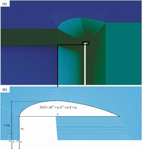
The mesh, containing about 500,000 elements, was built using the SALOME platform mesh generator, called “SMESH” (SALOME, www.salome-platform.org). A re-meshing strategy was adopted and meshes were automatically Python-script generated. Mesh settings were selected particularly to ensure sufficient refinement for all the generated geometries as presented in Figure 2. Meshes were refined around the weir (mesh size on the order of 1 mm) and in the free-surface zone upstream of the weir (mesh size of 4 mm).

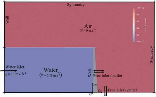
A flow discharge was set at the inlet boundary condition with a water depth equal to the weir height (i.e. $7.5H_d$). Downstream of the weir, a free output condition was applied to the horizontal sides. The lateral edge faces were symmetrical to model transverse invariance, and the other edge faces were walls (Figure 3). The computation time needed to achieve the stationary state varies according to the geometries tested, from 1 h to 3 h for a physical time lies within 12 s and 30 s on 28 bi-core Intel ®Xeon® processors, CPU E5-2680 [email protected] GHz.

Figure 3. Calculation domain and boundary conditions.

Finally, the objective function to be optimised was to minimise the weir head design $H_d$ for a fixed-design incoming flow discharge$q_d$. This is summarised by Equation (2):

(2) $H_d^{\ast }=min(H_d(q_d,\gamma ,\delta ,a_2,a_1))$(2)

Under constraint: $e>1/2$, with $q_d$ being the flow design discharge equal to that of a standard weir with a design head $H_d$of 0.2 m, calculated using Equations (3) and (4):

(3) $q_d=C_d\sqrt{2g{H}_d^3}$(3)

(4) $C_d=0.4950{\left(\frac{H}{H_d}\right)}^{0.12}$(4)

2.2. Hydrodynamic model

The numerical simulation used to compute water level is a 2D free-surface flow model at the local level of the spillway, implemented via the open-source CFD software Code_Saturne. The solver is based on a co-located finite-volumes type of discretisation (Archambeau et al., 2004) on unstructured meshes, which is suitable for a large variety of flows (e.g. incompressible or compressible; turbulent or not; with or without thermal transfers). The VOF method (Hirt & Nichols, 1981), described below, is used to keep track of the water–air interface.

The free surface or interface between two immiscible fluids is described by the characteristic function $\alpha$ of one of the fluids (the air in the present case). For a control volume $\mathrm{\Omega }$ of the discretised numerical domain, the average value of this characteristic function is equal to the volume fraction of air as defined by Equation (5):

(5) $\alpha =\frac{{\mathrm{\Omega }}_{air}}{\mathrm{\Omega }}$(5)

A homogeneous (or mono-fluid) approach is applied, for which a mass balance or linear momentum balance is worked out. The density $\rho$ and the dynamic viscosity $\mu$ of the mixed medium are defined by linear relations described by Equations (6):

(6) $\begin{array}{c}\mu =\alpha {\mu }_a+(1-\alpha ){\mu }_w\\ \rho =\alpha {\rho }_a+(1-\alpha ){\rho }_w\end{array}$(6)

with indices $a$ and $w$ referring to air and water, respectively.

The mass and momentum conservation equations are described by Navier-Stokes Equations (7):

(7) $\begin{array}{c}\frac{\mathrm{\partial }\rho }{\mathrm{\partial }t}+div(\rho \underset{\_}{u})=0\\ \frac{\mathrm{\partial }}{\mathrm{\partial }t}(\rho \underset{\_}{u})+\underset{\_}{div}(\underset{\_}{u}\otimes \rho \underset{\_}{u})=-\underset{\_}{\mathrm{\nabla }}P+\rho \underset{\_}{g}+\underset{\_}{div}(\underset{\_}{\underset{\_}{\tau }})\end{array}$(7)

where $\underset{\_}{u}$ is the mixed medium velocity vector, $P$ is the pressure, $\underset{\_}{g}$ is the gravity vector and $\underset{\_}{\underset{\_}{\tau }}=2\mu {\underset{\_}{\underset{\_}{S}}}^D$ is the Newtonian viscous stress tensor, with $\underset{\_}{\underset{\_}{S}}=\frac{1}{2}(\underset{\_}{\underset{\_}{\mathrm{\nabla }}}\underset{\_}{u}+\underset{\_}{\underset{\_}{\mathrm{\nabla }}}{\underset{\_}{u}}^T)$ as the strain rate tensor. Under the linearity hypothesis of density in relation to the volume fraction, the mass balance equation is equivalent to Equation (8):

(8) $\begin{array}{c}div(\underset{\_}{u})=0\\ \frac{\mathrm{\partial }\alpha }{\mathrm{\partial }t}+\underset{\_}{div}(\alpha \underset{\_}{u})=0\end{array}$(8)

Code_Saturne solves Equations (7)(7) $\begin{array}{c}\frac{\mathrm{\partial }\rho }{\mathrm{\partial }t}+div(\rho \underset{\_}{u})=0\\ \frac{\mathrm{\partial }}{\mathrm{\partial }t}(\rho \underset{\_}{u})+\underset{\_}{div}(\underset{\_}{u}\otimes \rho \underset{\_}{u})=-\underset{\_}{\mathrm{\nabla }}P+\rho \underset{\_}{g}+\underset{\_}{div}(\underset{\_}{\underset{\_}{\tau }})\end{array}$(7) and (8(8) $\begin{array}{c}div(\underset{\_}{u})=0\\ \frac{\mathrm{\partial }\alpha }{\mathrm{\partial }t}+\underset{\_}{div}(\alpha \underset{\_}{u})=0\end{array}$(8) ), which are discretised in time by an implicit Euler scheme. The velocity-and-pressure coupled system is solved by a fractional algorithm of prediction-correction type. Particular attention was given to spatial discretisation of the convection term of $\alpha$ of Equation (8) so that the physical limits (minimum–maximum principle) of $\alpha$ are respected. This avoids too large numerical diffusion and retains the fineness of the water–air interface. Several schemes have been implemented in Code_Saturne; in this study the numerical scheme M-CICSAM (Zhang et al., 2014) was used.

3. Surrogate model-based optimisation

The shape optimisation procedure implemented in this study was based on the use of a numerical model to compute the objective function. The numerical model requires substantial computing resources. Furthermore, the repetitive solution can be prohibitive in the context of an iterative optimisation procedure. To alleviate the computational burden, the optimisation procedure integrated a metamodel to be optimised by a metaheuristic algorithm (Figure 4). A detailed explanation of each method adopted during this optimisation study is presented in this section.

Figure 4. Surrogate-based optimisation procedure (~ above the head discharge H means estimated from the reduced-order model).

3.1. Reduced-order model

Due to the high computational cost of the CFD model in the optimisation loop, techniques of the reduced-order model (ROM) were implemented following four steps: (i) creation of a design of experiment, (ii) model on design of experiment points, (iii) metamodel construction and (vi) metamodel validation.

Two metamodels were tested. The first metamodel, by neural network, is based on a non-linear regression of outputs by a flexible stacking of functions with independent errors. The second approach, by kriging, on the contrary, adopts a simple form of regression (constant term) but considers a stochastic error method that allows consideration of correlated errors.

3.1.1. Metamodel by neural network method

A neural network of the multilayer-perceptron type is well adapted to non-linear relationships between inputs and one or more corresponding outputs. As discussed by Jones et al. (1998), this regression method supposes independence of errors. Indeed, in terms of the design of experiment $({\underset{\_}{p}}^i)$, the response of the simulator, designated by $Y_t$, at the point of the plan, $Y_t({\underset{\_}{p}}^i)=\mathrm{M}({\underset{\_}{p}}^i)$ is expressed according to Equation (9)(9) $Y_t({\underset{\_}{p}}^i)=\sum _k{\beta }_k{F}_k({\underset{\_}{p}}^i)+{\epsilon }^i,(i=1,\dots ,N)$(9) (where $\mathrm{M}$ designates the numerical model):

(9) $Y_t({\underset{\_}{p}}^i)=\sum _k{\beta }_k{F}_k({\underset{\_}{p}}^i)+{\epsilon }^i,(i=1,\dots ,N)$(9)

where $N$ is the learning sample size, $F_k$ is a class of non-linear functions of the input variables $\underset{\_}{p}=(p_1,\dots ,p_d)$, ${\beta }_k$ is the regression coefficients to be estimated and ${\epsilon }^i$ represents the errors assumed to be independent and distributed according to a normal law of average zero and variance ${\sigma }^2$.

A neural network is composed of multiple intermediary layers, each one containing neurons showing non-linear activation functions such as the “sigmoid” function $\left(\frac{1}{1+exp(-\underset{\_}{p})}\right)$ or rectified linear unit function ($max(0,\underset{\_}{p})$) (relu).

3.1.2. Metamodel by kriging method

Kriging is a geostatic technique of spatial modelling that enables homogeneous representation of the information studied (Matheron, 1963). It is often used to replace a computationally expensive model, starting with a certain number of points already evaluated by the actual code. In the present work, the deterministic response of the simulator $Y$ is considered to realise the random function described by Equation (10):

(10) $Y(\underset{\_}{p})=\beta +\mathrm{K}(\underset{\_}{p})$(10)

where $\underset{\_}{p}$ represents the vector of input variables, $\beta$ is an unknown parameter and $\mathrm{K}$ is a Gaussian process of zero expectation and covariance function given by Equation (11):

(11) $\begin{array}{c}Cov[K(\underset{\_}{p}),\mathrm{K}(\underset{\_}{q})]={\sigma }^{2}R(\underset{\_}{p},\underset{\_}{q})\\ R(\underset{\_}{p},\underset{\_}{q})=exp\left[-\sum _{i=1}^d{\theta }_i{(p_i-q_i)}^2\right],\mathrm{\forall }\underset{\_}{p},\underset{\_}{q}\in {\mathrm{\Re }}^d\end{array}$(11)

where ${\sigma }^2$ is the variance $R(\underset{\_}{p},\underset{\_}{q})$ and is the correlation function, with ${\theta }_i$ being an unknown parameter measuring the degrees of correlation following the direction $i$.

The parameters $(\beta ,{\sigma }^2,\underset{\_}{\theta })$ must be determined in order to estimate the metamodel through kriging. Starting with a design of experiment ${\underset{\_}{p}}^T=({\underset{\_}{p}}^1,\dots ,{\underset{\_}{p}}^N)$, the simulator responses on the points of the plan designated by ${{\underset{\_}{Y}}_t}^T=[\mathrm{M}({\underset{\_}{p}}^1),\dots ,\mathrm{M}({\underset{\_}{p}}^N)]$ are used to estimate the unknown parameters $(\beta ,{\sigma }^2,\underset{\_}{\theta })$ by the maximum likelihood method (the symbol $T$ means transposed). Maximum likelihood can be interpreted as an attempt to correlate the distribution of the model, defined by Equations (10)(10) $Y(\underset{\_}{p})=\beta +\mathrm{K}(\underset{\_}{p})$(10) and (11(11) $\begin{array}{c}Cov[K(\underset{\_}{p}),\mathrm{K}(\underset{\_}{q})]={\sigma }^{2}R(\underset{\_}{p},\underset{\_}{q})\\ R(\underset{\_}{p},\underset{\_}{q})=exp\left[-\sum _{i=1}^d{\theta }_i{(p_i-q_i)}^2\right],\mathrm{\forall }\underset{\_}{p},\underset{\_}{q}\in {\mathrm{\Re }}^d\end{array}$(11) ), with the empirical distribution from the simulated data ${\underset{\_}{Y}}_t$.

Once the kriging parameters are evaluated, it is then possible to estimate the response of the simulator and its variance at any point of the domain, according to Equation (12):

(12) $\begin{array}{c}\tilde{Y}=\tilde{\beta }+{\underset{\_}{r}}^T{\underset{\_}{\underset{\_}{R}}}^{-1}({\underset{\_}{Y}}_t-\underset{\_}{1}\tilde{\beta })\\ var[Y(\underset{\_}{p})]={\sigma }^2\left[1-{\underset{\_}{r}}^T{\underset{\_}{\underset{\_}{R}}}^{-1}\underset{\_}{r}+\frac{(1-{\underset{\_}{1}}^T{\underset{\_}{\underset{\_}{R}}}^{-1}\underset{\_}{1}}{{\underset{\_}{1}}^T{\underset{\_}{\underset{\_}{R}}}^{-1}\underset{\_}{1}}\right]\end{array}$(12)

where $\underset{\_}{\underset{\_}{R}}=R({\underset{\_}{p}}^i,{\underset{\_}{p}}^j{)}_{(i,j=1,\dots ,N)}$ is the matrix of correlations between the points of the design of experiment; $\underset{\_}{\underset{\_}{r}}=[R({\underset{\_}{p}}^1,\underset{\_}{p}),\dots ,R({\underset{\_}{p}}^N,\underset{\_}{p}){]}^T$ is the vector of correlations between $\underset{\_}{p}$ and the points of plan ${\underset{\_}{p}}^T$; $\underset{\_}{1}$ designates a size vector of the number of points in the plan containing only ones; and the symbol ~ above a letter, such as $\tilde{\beta }$, means “estimated”.

3.2. Optimisation algorithm

The optimisation algorithm chosen to improve the shape of the weir was the meta-heuristic particle swarm optimisation (PSO). This algorithm is sufficiently general to process any type of problems, even those that are of great size, non-linear and non-differentiable. This algorithm showed for the first time how to simulate social behaviour such as murmurations of birds or shoals of fish (Kennedy & Eberhart, 1995). It does not claim to find the global optimum of the minimisation or maximisation problem submitted. Moreover, no theory guarantees convergence. It has, however, proved its effectiveness in resolving optimisation problems under constraints, whether they are purely mathematical or coming from cases of practical study. Among recent hydraulic applications on a free surface, one can cite the calibration problem of the simulation model or that of optimal design research (Gœury et al., 2018).

PSO does not require calculation of derivatives, which can still pose problems of computation cost for large dimensions, or of accuracy linked to numerical rounding. The algorithm works with a set of candidate solutions (particles) randomly selected first from the space of variables for optimisation. Each particle represents a set of values, which in the present case defined a particular geometric shape of the weir. The rest of the algorithm tends to shift these particles towards the spatial area where the cost function corresponding to a particular flow behaviour is optimal. The desired optimisation concerns minimising the head above the weir. The algorithm shifts each particle forward iteratively with a velocity that depends on both the individual performance of the particle and the performance of the group (swarm).

4. Results

This section sets out the implementation of the preceding numerical optimisation procedure for the design needs of spillway design. In the first instance, two ROMs on which the optimisation was based were constructed and validated. Thereafter, the results from the optimisation process are presented and commented upon.

4.1. Learning and validating metamodels

As previously stated, the present optimisation study was achieved with the use of two metamodels, derived from a neural network approach and a kriging approach. To carry out this task, 1000 unit calculations, coming from an optimised Latin hypercube sampling (LHS) design of experiment (Damblin et al., 2013), were generated using the Python package OpenTURNS (Baudin et al., 2017). The number of calculations $N$ is far greater than the minimum number of calculations needed to obtain an accurate metamodel according to the empirical relationship $N\approx 10d$ (Marrel et al., 2009), since here the number of parameters to be optimised is $d=4$.

The neural network model was constructed using the Python package scikit-learn (Pedregosa et al., 2011), and the kriging model was constructed using its implementation in OpenTURNS (Baudin et al., 2017). To validate the resulting metamodels’ accuracy, a “leave-one-out” validation procedure was used (Arlot & Celisse, 2010), in which on test $i$, the “$i$”th datum of the design of experiment is removed from the learning sample. A ROM is then estimated from this learning database. Then, using this new model, the predicted value at the “$i$”th test point is estimated $\tilde{Y}({\underset{\_}{p}}^i)$ and different errors can be calculated:

• Average bias: $\frac{1}{N}\sum _{i=1}^N\mathrm{M}({\underset{\_}{p}}^i)-\tilde{Y}({\underset{\_}{p}}^i)$

• Mean squared error: $MSE=\frac{1}{N}\sum _{i=1}^N{(\mathrm{M}({\underset{\_}{p}}^i)-\tilde{Y}({\underset{\_}{p}}^i))}^2$

• Productivity coefficient: $Q^2=1-\frac{\sum _{i=1}^N\mathrm{M}({\underset{\_}{p}}^i)-\tilde{Y}({\underset{\_}{p}}^i)}{var[\mathrm{M}(\underset{\_}{p})]}$

While adjusting surrogate model parameters (e.g. number of layers, number of neurons per layer, and the activation function for the neural network model or the regression function and covariance functions for the kriging model), the focus was on the predictability criterion $Q^2$ for a test set, and the configuration with the best criterion was chosen. As a result, for kriging, the retained metamodel comprised the constant regression function and the stochastic part of absolute exponential covariance (Equations (11)(11) $\begin{array}{c}Cov[K(\underset{\_}{p}),\mathrm{K}(\underset{\_}{q})]={\sigma }^{2}R(\underset{\_}{p},\underset{\_}{q})\\ R(\underset{\_}{p},\underset{\_}{q})=exp\left[-\sum _{i=1}^d{\theta }_i{(p_i-q_i)}^2\right],\mathrm{\forall }\underset{\_}{p},\underset{\_}{q}\in {\mathrm{\Re }}^d\end{array}$(11) –(12(12) $\begin{array}{c}\tilde{Y}=\tilde{\beta }+{\underset{\_}{r}}^T{\underset{\_}{\underset{\_}{R}}}^{-1}({\underset{\_}{Y}}_t-\underset{\_}{1}\tilde{\beta })\\ var[Y(\underset{\_}{p})]={\sigma }^2\left[1-{\underset{\_}{r}}^T{\underset{\_}{\underset{\_}{R}}}^{-1}\underset{\_}{r}+\frac{(1-{\underset{\_}{1}}^T{\underset{\_}{\underset{\_}{R}}}^{-1}\underset{\_}{1}}{{\underset{\_}{1}}^T{\underset{\_}{\underset{\_}{R}}}^{-1}\underset{\_}{1}}\right]\end{array}$(12) )). The metamodel coming from the neural network comprised five layers, each containing 140 neurons and “relu” as the activation function. Table 2 summarises the results of the “leave-one-out” validation for the two constructed metamodels.

Table 2. Values of validation criteria for each metamodel

Metamodel	$Q^2$	Average bias	MSE
Kriging	0.95	1.5e-6	6.0e-6
Neural network	0.97	−7.0e-6	4.0e-6

The two surrogate models were validated according to the performance criteria described above. Crossed validation gives results close to zero for the average bias and the quadratic error, while the productivity criterion $Q^2$ is approximately 0.95. As a reminder, a coefficient $Q^2$ close to 1 shows a good fit between the learning database and the result estimated by the ROM. According to Viana et al. (2009), a ROM with a predictive coefficient higher than 0.9 can be considered satisfactory in a study framework. Thus, the two ROMs were retained and used in what follows in implementing the shape optimisation procedure.

4.2. Spillway’s optimal shapes

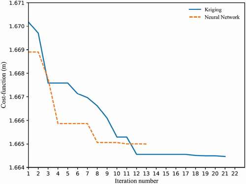
A swarm of 40 particles was considered and the optimisation process was carried out several times to ensure that the optimal solution is stationary. Since, PSO, by construction, is a non-constrained algorithm, the geometric constraint (weir thickness: Equation (3)(3) $q_d=C_d\sqrt{2g{H}_d^3}$(3) ) was enforced using a penalty function (Parsopoulos & Vrahatis, 2002). The algorithm stops when the swarm has converged towards a zone of space that improves the weir’s geometry. This improvement is conventionally evaluated from the database of a maximum number of iterations or the stationarity of the cost function. Figure 5 shows the evolution of the global best swarm position at each iteration. It should be noted that at each iteration, the swarm is evaluated as a whole. Each iteration then requires 40 parallel calculations of the hydraulic simulator, the simulator being one of the ROMs constructed beforehand.

Figure 5. Particle swarm optimisation algorithm convergence curve for ogee-crest weir using kriging and neural network models.

The optimal weir shapes obtained after the optimisation process are shown in Figure 6, and their parametric and physical results are recapped in Table 3. The minimum head upstream of the various optimised weirs showed a similar gain on the order of 17% compared to a standard weir. Even though they were mathematically based on different error models, the two metamodels demonstrated analogous performance and resulted in a net improvement in head after optimisation. The predicted head for each of the metamodels was compared to those computed by Code_Saturne. The results obtained showed an absolute error of 1%, confirming the metamodels’ accuracy. On the other hand, the fact that no parameter was located on the boundary of the domain allowed a posteriori verification of the search domain.

Table 3. Results of the optimisation process

Optimisation method	Kriging	ANN
Parameters	$\gamma$ = 1.2807; $\delta$ = 0.2210 a2 = −2.4571; a1 = −1.2156	$\gamma$ = 1.4411; $\delta$ = 0.1913 a2 = −3.8995; a1 = −0.8889
Weir head (m)	0.164	0.165
Head calculated with Code_Saturne (m)	0.165	0.164
Gap	−0.06%	0.06%
Percentage gain in head compared to standard weir	17.5%

Figure 6. Comparison of resulting optimal shapes.

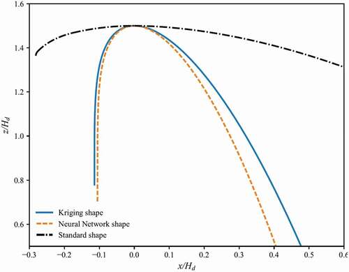
Although the results are analogous in terms of hydraulic head, the two shapes obtained by the optimisation process displayed differences, as shown in Figure 6. This demonstrates the multi-modal aspect of the optimisation: there were several solutions that were close in the results space (hydraulic head) but differed in the parameter space. Figure 6 shows, however, that the differences were essentially focused on the downstream quadrant. Thus, as specified by Erpicum et al. (2019) and in view of the shape optimisation results, it appears that hydraulic head is mainly influenced by the upstream quadrant shape.

5. Discussion

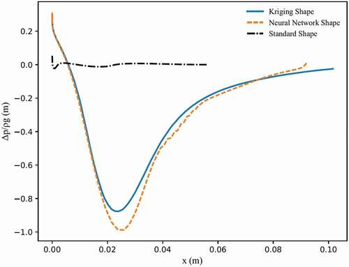
The studied shape optimisation of ogee-crested overflow weirs shows satisfying and promising results, with expected gains of more than 17% of the discharge coefficient. However, during the mono-objective optimisation process a second design criterion was omitted and should be considered at this stage. In fact, for a fixed design discharge (H/H_d = 1), a standard ogee weir does not develop negative pressure along its crest, unlike the optimised weirs (as illustrated in Figure 7). Figure 7 shows that along optimised weir shapes, the minimum relative pressure is between −0.9 m and −1 m. The origin of the x benchmark in Figure 7 is at the upstream face of the weir. Furthermore, for a hydraulic head greater than the design head, Hager and Schleiss (2009) showed that for a standard weir, negative pressure appears along the crest, but the discharge coefficient continues to increase. Therefore, it seems more pertinent to compare our results to a standard weir under negative pressure conditions equivalent to those that are obtained for the optimised shapes.

Figure 7. Pressure profiles along weirs.

Erpicum et al. (2019) presented profiles of relative pressure along a standard weir based on the relationship H/H_d. The geometries obtained by the optimisation procedure showed negative pressure equivalent to a standard weir for which the relationship H/H_d is equal to about 3. A few authors have estimated the coefficient $C_d$ for standard weir flows where the head exceeds the head design (notably Cassidy, 1970; Erpicum et al., 2018; Hager & Schleiss, 2009; USACE, 1977; Vermeyen, 1991). Table 4 covers these data for the relationship H/H_d = 3. In light of the results, the expected gain in $C_d$ for these optimised geometries is between 8% and 15%.

Table 4. Comparison between discharge coefficients of a standard weir under negative pressure conditions and optimised weirs

Ref.	Discharge coefficients (Cd)
Hager and Schleiss (2009)	0.56
USACE (1977)	0.57
Vermeyen (1991)
Erpicum et al. (2018)
Cassidy (1970)	0.60
Optimal shapes (this work)	0.648

It should be noted that the appearance of negative pressure is a source of cavitation problems that could elicit structural damage. To limit this, complementary studies must be carried out. In fact, as Figure 7 shows, although the two shapes have the same coefficient discharge, the peak of minimum pressure varies by approximately 10%. That means weir negative pressure can be limited by directly integrating it as a second objective to be optimised. A multicriterion optimisation can then be implemented via a genetic-type metaheuristic algorithm to determine the Pareto front.

6. Conclusions

Although studied for almost a century, standard weirs have yet to undergo shape optimisation. In this paper, we parametrised the weir geometry through an analytical expression, carried out a set of Code_Saturne simulations according to design of experiment (LHS) and constructed two metamodels: one by kriging and the other by neural network learning. Finally, from these metamodels, we made use of the PSO optimisation algorithm to propose new geometries for weir spillways. We worked with a constant discharge of 0.196 m³ s⁻¹, which corresponds to a dimensioning head for a standard weir of 0.2 m. In the first instance, we compared the water level obtained at this head. The optimised shapes allowed us to lower the water surface by 17.5%. Nevertheless, these new geometries generated subpressure on the weir for the discharge head we had set. As a new means of comparison, still for a discharge of 0.196 m³ s⁻¹, we selected a standard weir with dimensions that induce subpressure equivalent to that obtained for the optimised geometries. This time, for the discharge coefficient, the gains were between 8% and 15%.

The numerical tools used in this study are generic and can be used to optimise other spillway shapes, such as the piano-key weir, thereby becoming effective design tools for the engineer. In fact, the use of a CFD code, a ROM and a metaheuristic optimisation algorithm makes the optimisation chain developed independent of the configuration studied and the meshing part. As a result, for new geometries and design parameters, one could generate the experiment plan, run the CFD code, then construct and validate the ROM, and finally run the optimisation algorithm in search for the optimal solution. The developed optimisation methodology could be enhanced by integrating pressure distribution as a second optimisation criterion and taking into account uncertainty factors (e.g. geometrical parameters, initial conditions). A robust multi-criterion optimisation is therefore envisaged in an upcoming work. Once implemented, the shape optimisation results can then be validated experimentally with the optimal shapes obtained directly by 3D printing.

Disclosure statement

No potential conflict of interest was reported by the authors.

Additional information

Notes on contributors

Fatna Oukaili

Fatna Oukaili is a PhD student National Laboratory for Hydraulics and Environment, EDF R&D, Chatou.

Yvan Bercovitz

Yvan Bercovitz is an Engineer-Researcher at National Laboratory for Hydraulics and Environment, EDF R&D, Chatou.

Cédric Goeury

Cédric Goeury is an Engineer-Researcher at  National Laboratory for Hydraulics and Environment, EDF R&D, Chatou.

Fabrice Zaoui

Fabrice Zaoui is an Engineer-Researcher at National Laboratory for Hydraulics and Environment, EDF R&D, Chatou.

Erwan Le Coupanec

Erwan Le Coupanec is an Engineer-Researcher at Fluid Dynamics, Energy and Environment Department, EDF R&D, Chatou.

Kamal El kadi Abderrezzak

Kamal El Kadi Abderrezzak is an Engineer-Researcher at  National Laboratory for Hydraulics and Environment, EDF R&D, Chatou.

References

- Abecasis, F. M. (1970). Discussion of designing spillway crests for high-head operation. Journal of the Hydraulics Division, 96(12), 2654–2658. https://doi.org/https://doi.org/10.1061/JYCEAJ.0002821
- Alvarez-Vázquez, L. J., Martinez, A., Vázquez-Méndez, M. E., & Vilar, M. A. (2006). Numerical resolution of a shape optimization problem in hydraulic engineering Proceedings of the European conference on computational fluid dynamics, Delft, Netherlands.
- Archambeau, F., Mechitoua, N., & Sakiz, M. (2004). Code_Saturne: A finite volume code for the computation of turbulent incompressible flows – Industrial applications. International Journal on Finite Volumes, 1(1). https://hal.archives-ouvertes.fr/hal-01115371
- Arlot, S., & Celisse, A. (2010). A survey of cross-validation procedures for model selection. Statistical Surveys, 4, 40–79. https://doi.org/https://doi.org/10.1214/09-SS054
- Baudin, M., Dutfoy, A., Iooss, B., & Popelin, A.-L. (2017). OpenTURNS: An industrial software for uncertainty quantification in simulation. In R. Ghanem, D. Higdon & H. Owhadi (Eds.), Handbook of uncertainty quantification (pp. 2001–2038). Springer.
- Bazin, H. (1898). Expériences sur l’écoulement en déversoir exécutées à Dijon de 1886 à 1895. Dunod.
- Cassidy, J. J. (1970). Designing spillway crests for high-head operation. Journal of Hydraulic Division, 96(3), 745–753. https://doi.org/https://doi.org/10.1061/JYCEAJ.0002376
- Creager, W. P. (1917). Engineering for masonry dams. John Wiley and Sons.
- Damblin, G., Couplet, M., & Iooss, B. (2013). Numerical studies of space filling designs: Optimization of Latin hypercube samples and subprojection properties. Journal of Simulation, 7(4), 276–289. https://doi.org/https://doi.org/10.1057/jos.2013.16
- Dargahi, D. (2006). Experimental study and 3D numerical simulations for a free-overflow spillway. Journal of Hydraulic Engineering, 132(9), 899–907. https://doi.org/https://doi.org/10.1061/(ASCE)0733-9429(2006)132:9(899)
- De Marchi, G. (1928). Ricerche sperimentali sulle dighe tracimanti. Annali dei lavori pubblici. Il profile delle dighe sfioranti. L’energia Elettrica, 7(14), 937–940.
- Elchahal, G., Younes, R., & Lafon, P. (2013). Optimization of coastal structures: Application on detached breakwaters in ports. Ocean Engineering, 63, 35–43. https://doi.org/https://doi.org/10.1016/j.oceaneng.2013.01.021
- Erpicum, S., Archambeau, P., Dewals, B., & Pirotton, M. (2009). Automatic geometrical optimization by way of numerical flow models. In Advances in Water Resources and Hydraulic Engineering (pp. 1663–1668). Springer. https://doi.org/https://doi.org/10.1007/978-3-540-89465-0_287
- Erpicum, S., Blancher, B., Peltier, Y., Vermeulen, J., Archambeau, P., Dewals, B., & Pirotton, M. (2018). Experimental study of ogee crested weir operation above the design head and influence of the upstream quadrant geometry. 7th international symposium on hydraulic structures, Aachen, Germany.
- Erpicum, S., Pirotton, M., Blancher, B., & Vermeulen, J. (2019). Influence de la géométrie du quadrant amont et comportement hydraulique sous forte charge des seuils profilés standards. La Houille Blanche, 105(1), 40–47. https://doi.org/https://doi.org/10.1051/lhb/2019006
- Ferdowsi, A., Farzin, S., Mousavi, S.-F., & Karami, H. (2019). Hybrid bat & particle swarm algorithm for optimization of labyrinth spillway based on half & quarter round crest shapes. Flow Measurement and Instrumentation, 66, 209–217. https://doi.org/https://doi.org/10.1016/j.flowmeasinst.2019.03.003
- Gœury, C., Zaoui, F., Audouin, Y., Prodanovic, P., Fontaine, J., Tassi, P., & Ata, R. (2018). Finding good solutions to telemac optimization problems with a metaheuristic. Proceedings of 25th TELEMAC-MASCARET user conference, Norwich, UK.
- Hager, W. H., & Castro-Orgaz, O. (2017). Ogee weir crest definition: Historical advance. Proceedings of the 37th IAHR world congress, Kuala Lumpur, Malaysia.
- Hager, W. H., & Schleiss, A. J. (2009). Constructions hydrauliques : Ecoulements stationnaires. Presses Polytechniques et Universitaires Romandes (PPUR).
- Hirt, C. W., & Nichols, B. D. (1981). Volume of Fluid (VOF) method for the dynamics of free boundaries. Journal of Computational Physics, 39(1), 201–225. https://doi.org/https://doi.org/10.1016/0021-9991(81)90145-5
- Hosseini, K., Nodoushan, E. J., Barati, R., & Shahheydari, H. (2016). Optimal design of labyrinth spillways using meta-heuristic algorithms. KSCE Journal of Civil Engineering, 20(1), 468–477. https://doi.org/https://doi.org/10.1007/s12205-015-0462-5
- Imanian, H., & Mohammadian, A. (2019). Numerical simulation of flow over ogee crested spillways under high hydraulic head ratio. Engineering Applications of Computational Fluid Mechanics, 13(1), 983–1000. https://doi.org/https://doi.org/10.1080/19942060.2019.1661014
- Jones, D. R., Schonlau, M., & Welch, W. J. (1998). Efficient global optimization of expensive black-box functions. Journal of Global Optimization, 13(4), 455–492. https://doi.org/https://doi.org/10.1023/A:1008306431147
- Kennedy, J., & Eberhart, R. (1995). Particle swarm optimization. Proceedings of the 4th IEEE international conference on neural networks, Perth, Australia.
- Marrel, A., Iooss, B., Laurent, B., & Roustant, O. (2009). Calculations of the sobol indices for the Gaussian process metamodel. Reliability Engineering and System Safety, 94(3), 742–751. https://doi.org/https://doi.org/10.1016/j.ress.2008.07.008
- Matheron, G. (1963). Principles of geostatistics. Economic Geology, 58(8), 1246–1266. https://doi.org/https://doi.org/10.2113/gsecongeo.58.8.1246
- Müller, R. (1908). Development of a practical type of concrete spillway dam. The Engineering Record, 58(17), 461–462.
- Parsopoulos, K., & Vrahatis, M. (2002). Particle swarm optimization method for constrained optimization problem. In Intelligent technologies – theory and applications:New trends in intelligent technologies (pp. 214–220).
- Pedregosa, F., Varoquaux, G., Gramfort, A., Michel, V., Thirion, B., Grisel, O., Blondel, M., Prettenhofer, P., Weiss, R., Dubourg, V., Vanderplas, J., Passos, A., Cournapeau, D., Brucher, M., Perrot, M., & Duchesnay, E. (2011). Scikit-learn: Machine learning in Python. Journal of Machine Learning Research, 12, 2825–2830. https://doi.org/https://doi.org/10.5555/1953048.2078195
- Scimeni, E. (1937). Il profile delle dighe sfioranti. L’energia Elettrica, 14(12), 937–940.
- United States Army, Corps of Engineers. (1977) . Hydraulic design criteria.
- Vermeyen, T. B. (1991). Hydraulic model study of Ritschard dam spillways. U.S. Department of Interior.
- Viana, F. A. C., Haftka, R. T., & Steffen, J. V. (2009). Multiple surrogates: How cross-validation errors can help us to obtain the best predictor. Structural and Multidisciplinary Optimization, 39(4), 439–457. https://doi.org/https://doi.org/10.1007/s00158-008-0338-0
- Zarfl, C., Lumsdon, A. E., Berlekamp, J., Tydecks, L., & Tockner, K. (2015). A global boom in hydropower dam construction. Aquatic Sciences, 77(1), 161–170. https://doi.org/https://doi.org/10.1007/s00027-014-0377-0
- Zhang, D., Jiang, C., Liang, D., Chen, Z., Yang, Y., & Shi, Y. (2014). A refined VOF algorithm for capturing sharp fluid interfaces on arbitrary meshes. Journal of Computational Physics, 274, 709–736. https://doi.org/https://doi.org/10.1016/j.jcp.2014.06.043