Uncertainty quantification and global sensitivity analysis with dependent inputs parameters: Application to a basic 2D-hydraulic model

ABSTRACT

Hydraulic models include many uncertainties related to model parameters. Uncertainty Quantification (UQ) and Global Sensitivity Analysis (GSA) allow to quantify these uncertainties and identify the most influent parameters. To use traditional methods of UQ and GSA, the inputs must be independent. Therefore, this research aims to show that the dependence between inputs should not be neglected in uncertainty studies. To illustrate this, we used a simple hydraulic model built with TELEMAC-2D, representing a hypothetical linear river protected by a dyke that can break. The methodology is completed following these steps: the uncertain inputs and the outputs of interest are identified. Then, the inputs margins are defined through a statistical analysis using real dataset. The dependence structure between inputs is figured using copulas. Kriging metamodels are used to increase the number of experiences in a short time period. Finally, UQ and GSA are achieved. Regarding the UQ results, the outputs distribution is different if the inputs are considered dependent or not, whereas regarding the GSA, some parameters, usually considered non-influent in the hypothesis of independent inputs, have a real impact on the outputs. These results suggest that it could be interesting to consider the dependencies between inputs for “real” applications.

RÉSUMÉ

Les modéles hydrauliques comportent de nombreuses incertitudes liées aux paramétres du modéle. La quantification de l’incertitude (UQ) et l’analyse de sensibilité globale (GSA) permettent de quantifier ces incertitudes et d’identifier les paramétres les plus influents. Pour utiliser les méthodes traditionnelles de UQ et de GSA, les entrées doivent être indépendantes. Cette recherche vise à montrer que la dépendance entre les intrants ne doit pas être négligée dans les études d’incertitude. Pour illustrer cela, nous avons utilisé un modéle hydraulique simple construit avec TELEMAC-2D, représentant une hypothétique riviére linéaire protégée par une digue qui peut se rompre. La méthodologie est complétée selon les étapes suivantes: les incertitudes sur les entrées et les sorties pertinentes sont identifiées. Ensuite, les marges d’entrée sont définies via une analyse statistique utilisant un jeu de données réel. La structure de dépendance entre les entrées est figurée à l’aide de copules. Les métamodéles de krigeage sont utilisés pour augmenter le nombre d’expériences sur une courte période de temps. Enfin, les techniques de UQ et de GSA sont mises en oeuvre. Concernant les résultats UQ, la distribution des sorties est différente si les entrées sont considérées comme dépendantes ou non, alors que concernant l’approche GSA, certains paramétres, habituellement considérés comme non influents dans l’hypothése d’entrées indépendantes, ont un réel impact sur les sorties. Ces résultats suggérent qu’il pourrait être intéressant de considérer les dépendances entre les entrées pour des applications « réelles ».

KEYWORDS:

• Dependent parameters
• uncertainty quantification
• global sensitivity analysis
• 2D hydraulic model
• copula
• metamodel

MOTS CLÉS:

• Paramétres dépendants 
• Quantification d’incertitudes 
• Analyse de sensibilité globale 
• Modéle hydraulique 2D 
• Copules 
• Méta-modéle

1. Introduction

Flooding hazard is usually assessed through numerical modelling. However, models include many uncertainties related, in part, to the model input parameters. Especially, the prediction of hydraulic (i.e. roughness coefficients and hydrograph parameters) and breach parameters (i.e. location, geometry) is an important source of uncertainty impacting the water level at a given location. Thus, there is a need to better understand the impact of uncertain inputs, on the generated overflows. In order to improve the quantification of the flooding hazard and to better understand the uncertainties, Uncertainty Quantification (UQ) and Global Sensitivity Analysis (GSA) can be used. Traditionally, to perform these kinds of analyses, the model input parameters are supposed to be independent, which is not always the case, especially in hydraulic studies. Therefore, this study aims to illustrate that the dependence between inputs should not be neglected in uncertainty analyses.

Methods based on statistical techniques have been developed to deal with uncertainties in hydraulic model (Bacchi, Duluc et al., 2018). Current method to validate models and identify influencing parameters is to perform a UQ as well as a GSA (Iooss et al., 2013; Saltelli et al., 2008). UQ attempts to describe the entire set of possible outcomes considering that the input system is not perfectly known while the GSA attempts to describe how much model outputs are affected by changes in model inputs. The GSA is often used to rank parameters. Regardings method to consider sources of breach parameters uncertainties, Monte Carlo method/approach, also called uncertainty propagation, is commonly used in the hydraulic community (Apel et al., 2008; Domeneghetti et al., 2013; Korswagen et al., 2019; Sanyal, 2017).

While traditional methods as the Monte Carlo one, are frequently used to process UQ with inputs considered being independent, methods including copulas can be deployed to deal with dependent inputs. Instead of randomly sample inputs only inside parameter distributions, a dependence concept can be added and the inputs can be randomly sampled also inside copulas. Knowing the dependencies between parameters, copulas can be created. A copula is a joint distribution defined in a d-dimensional space [0,1]^d with uniform marginal distributions (Nelsen, 2007), d being the number of parameters inside the given copula. Copula are frequently used in multivariate flood frequency analyses and some authors use copula approaches to model the dependence structure, between hydrograph parameters for instance (Balistrocchi etal.; Domeneghetti et al., 2013; Vorogushyn et al., 2011).

Regarding the GSA, new methods have been recently developed to take into account the dependencies between inputs (Jacques et al., 2006; McKay, 1995; Ratto et al., 2005; Saltelli et al., 2004; Da Veiga et al., 2009). For instance, Li & Mahadevan propose to compute the first order Sobol’ index, using the variance decomposition (Li & Mahadevan, 2016) and Owen & Prieur (Owen & Prieur, 2016) and Iooss & Prieur (Iooss & Prieur, 2018) introduced the Shapley effects to take into account the dependence between inputs in GSA.

Such methods require a large number of simulations and can demand large computational time when 2D model are used. Therefore, alternative methods, such as metamodel approaches, can be used to drastically reduce the times of calculation (Bacchi, Richet et al., 2018; Fang et al., 2005; Richet & Bacchi, 20192019).

Previous studies have been carried out to investigate levee breach influence on flooded areas with HEC-RAS 1D (Bertrand et al., 2018; Pheulpin et al., 2019, 2020) and TELEMAC-2D (Pheulpin et al., 2020) models along the Garonne River. UQ and GSA have been conducted to evaluate the sensitivity of flooding associated to levee breaches and the influence of breach parameters related to overtopping, on the water levels within storage areas. Metamodels were used to reduce the computational time for the models and the 1D and 2D models were compared in terms of UQ and GSA. The study show the strong influence of the overflow parameter and the one of the breach geometry parameters, on the water height in a given storage area. The study also highlights the major difference between upstream and downstream parts of the river. Indeed, the upstream area is much more sensitive to levee breaches than the downstream area, so the uncertainties on maximum water levels are higher. These previous studies identified the need to carry out similar analyses by taking into account the dependencies between inputs and to integrate all the uncertain inputs (hydraulic and breach parameters) in the same study.

In this context, the objective of this work is to propose a methodology to proceed a complete uncertainty analysis including UQ and GSA and taking into account the dependencies between model inputs. Here the methodology is applied to a very simple case of inundation modelled with TELEMAC-2D and it will be applied to large hydraulic models in a near future. This paper is divided in the following parts: the second part presents the case study, the third part introduces the methodology and the fourth part shows the results of the UQ and GSA with dependent inputs or independent.

2. Presentation of the case study

The case study is a simplified 2D model of inundation built with TELEMAC-2D. This model is available in the TELEMAC-2D “examples” (Hervouet & Ata, 2017). A 5 km length fictive river is lined with a 1 km length dyke on the left bank. Behind this dyke there is a floodplain which can be flooded (Figure 1). The model mesh contains 26,450 elements and one run of this model lasts, on average, 1 minute and 30 seconds to simulate a 4 hours flood with 64 processors. The objective is to simulate a dyke breach considering different input parameters, in order to process an uncertainty analysis.

Figure 1. Illustration of the case study in 2D and 3D views. The 3D view shows the bottom mesh at the end of the simulation. The points P7, P9, P18 and P20 corresponds to the outputs of interest.

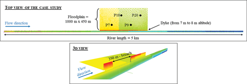
Here, we only focuses on four outputs corresponding to the maximum water level at four points located in the floodplain (P7, P9, P18 and P20 in Figure 1).

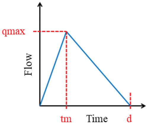
The uncertain input parameters of this model, which are uncontrolled (i.e. they cannot be controlled by humans contrary to the the dyke height for instance), are the hydraulic parameters and the breach parameters. The first ones correspond to the rugosity coefficient or Strickler coefficient (ks), which is a calibration parameter and to the hydrograph parameters shown in Figure 2 (maximum flow (qmax), time to peak (tm) and duration (d) of the flood). To simplify the calculations, we use a triangular hydrograph as upstream limit conditions and a linear rating curve to convert the flow into water level.

Figure 2. Hydrograph with 3 uncertain inputs: maximum flow (qmax), time to peak (tm) and duration (d) of the flood.

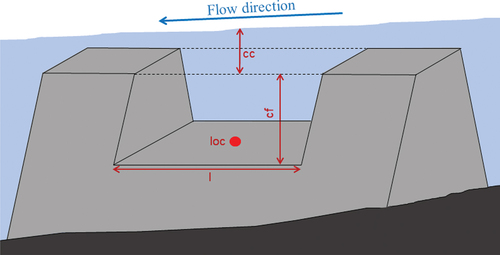
The second parameter category corresponds to the breach parameters (Figure 3). Here, we consider that the dyke breaches when the water level above the dyke (at the breach centre) reaches a given level (uncontrolled parameter cc). Then, the breach is opening by widening for a given time period (uncontrolled parameter do). The breach centre is also considered as an uncontrolled parameter and corresponds to the longitude (loc) of the breach centre (n.b. the dyke latitude is constant). Finally the last breach parameters are the final breach dimensions: the final length (l) and final depth (cf).

Figure 3. Illustration of the 4 breach parameters: control level (cc), final depth (df), final length (l) and location (loc) corresponding to the breach centre longitude. The last breach parameter, the opening duration (do) is not represented in this figure.

3. Methodology

3.1. Definition of uncertain inputs and dependencies

As the objective is to simulate a certain number of floods with different combinations of random parameters, it is first necessary to determine the Probability Density Functions (PDF) of all inputs and the dependencies between them. Knowing the PDF of all inputs and the copulas (cf. definition in the Introduction), we will be able to generate a random sample of inputs. Generally the PDF and the dependencies are defined using real dataset. Here, as we simulate a hypothetical flood, we chosed to use the same PDF and copulas than the ones used for the Loire River (paper in progress: application of this methodology to the Loire River), but with ranges adapted to this case study.

3.1.1. Hydraulic parameters

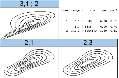
As the Strickler coefficient (ks) is a calibration parameter, a uniform distribution is used and this parameter is always considered as independent. For the hydrograph parameters, a truncated Gumbel distribution is used for the maximum flow (qmax), and truncated log normal distributions are used for the duration (d) and time to peak (tm). In fact, from the real dataset of the Loire River in Gien, we extracted the main floods and determined that these distributions well reprensents the hydrograph parameter distributions. Concerning the dependencies between the hydrograph parameters, a Vine model is used (Mazo, 2014). To model the dependencies between 3 inputs, the Vine models (high dimensions copulas) are more appropriate than the “classical” multivariate copulas. This Vine model was determined using the Loire River dataset and the R package VineCopula (Nagler et al., 2019). The most appropriated Vine model (including 3 copulas) and its parameters is represented in Figure 4.

Figure 4. Vine model representation used to model the dependencies between hydrograph parameters. The parameter 1 corresponds to the duration, 2 is the maximum flow and 3 is the time to peak.

3.1.2. Breach parameters

For the breach parameters, it is more complicated to define the PDF and the dependencies as there is a lack of data. Concerning the opening duration (do), as we have no real data, we consider a uniform distribution and no dependence with other parameters. For the location and control level of breach, we also use uniform distributions as we have no real data, but here we consider these two inputs dependent. The dependence is modelled with a Gaussian copula having one parameter (equal to −0.96). Finally for the dimension breach parameters (l and cf), we use truncated log normal distributions determinded using a breach dataset coming from known breaches betwenn Gien and Orléans in the Loire River (DREAL Centre, 2011). This dataset also allows to find a dependency between the breach dimensions; a survival Tawn type 2 copula with two parameters (3.02 and 0.48) is used.

Finally, all the inputs are randomly sampled inside the PDF presented in Table 1 and using the copula mentioned here. The minimum and maximum boundaries are arbitrarily chosen. Among others, qmax max. is not too high otherwise we would not see the breach effect, tm max. has to always be under d and cc max. is selected in such a way as the dyke breaches with an overflow of 20 cm max.

Table 1. Inputs distributions and copulas.

Inputs	PDF	Distribution parameters		Copula
ks	uniform	min	10	–
		max	20
d	truncated log-normal	mean(log)	6000	Vine model
		sd(log)	1000
		min	4500
		max	14,400
tm	truncated log-normal	mean(log)	2000
		sd(log)	500
		min	900
		max	3600
qmax	truncated Gumbel	location	200
		scale	100
		min	250
		max	600
do	uniform	min	0	–
		max	4500
loc	uniform	min	2200	Gaussian copula
		max	2800
cc	uniform	min	7,2
		max	8
l	truncated log-normal	mean(log)	5	Survival Tawn type 2
		sd(log)	0,75
		min	30
		max	400
cf	truncated log-normal	mean(log)	1,75
		sd(log)	0,6
		min	2
		max	6,9

3.2. Simulations with TELEMAC-2D

Once we know the inputs distributions and the dependencies between them, we can launch a large number of calculations with TELEMAC-2D. However, to proceed an uncertainty analysis, we need a very large dataset (here we want to use a dataset of 1000 calculations), that is why we only launch 200 runs with TELEMAC-2D before to use metamodels to built larger datasets.

We created an experimental design of 200 combinations of parameters. Here the inputs are randomly sampled inside uniform distributions (parameters ranges in Table 2) and without taking into account the dependencies. To lauch the 200 calculations successively and to extract the maximum water level at the 4 points of interest, we used the IRSN computational tool Funz (https://funz.github.io/doc/) which can be coupled with the software TELEMAC-2D.

Table 2. Ranges of input parameters.

	ks [-]	qmax [m^3/s]	tm [s]	d [s]	do [s]	cf [m]	cc [m]	l [m]	loc [m]
Min	10	250	900	4500	0	2	7.2	30	2200
Max	20	600	3600	14,400	4500	6.9	8	400	2800

The 200 runs with TELEMAC-2D lasted 2 hours and 50 minutes (with 64 processors). We could have launched the 1000 simulations only with TELEMAC-2D, but the objective is to establish a general methodology which will be applied to the model of the Loire River for which one simulation lasts 2 hours on average.

3.3. Metamodels building

Contrary to the 2D hydraulic model which observes the flow physics, the metamodels are mathematical approximations of the numerical model built on a learning basis. Metamodels are currently used for UQ and GSA approaches as they allow to drastically reduce the computational time yet preserving the quality of the statistical results of the original model. For our analysis, a Gaussian process, also called kriging metamodel has been selected (Gratiet et al., 2016) for its good predictive capacities ever demonstrated (Marrel et al., 2008). The methodology employed for the construction and the validation of metamodels is fully detailed in previous studies (Saltelli, 2002; Wahl, 2004).

Here we built 4 metamodels, one for each output, following these 3 main steps:

1. Building of a learning basis corresponding to the dataset with the 200 combinations of 9 inputs and 4 outputs with the coupling tool Funz/TELEMAC-2D (cf. part 3.2);

2. Building of the 4 kriging metamodels using the learning basis with the R package DiceEval (Dupuy et al., 2015). The theoretical background for kriging meta-model design used in this study is fully detailed in (Roustant et al., 2012);

3. Validation and accuracy of metamodels. To validate the metamodels, we used k-fold cross-validation and leave-one-out cross validation methods (details in Pheulpin et al. (2020)) and to check the accuracy, we used the R-squared, representing the squared correlation between the observed values (from the hydraulic model) and the predicted ones (from the metamodel). The higher the adjusted R² is, the better the model is. We also used the Root Mean Squared Error (RMSE) and the Mean Absolute Error (MAE). The lower the RMSE and MAE are, the better the model is.

3.4. Uncertainty Quantification (UQ)

Once the four metamodels built, we can proceed with the UQ. For this, 2 new experimental designs of 1000 simulations each are built. The inputs are randomly sampled inside the distributions presented in Table 1, considering the inputs being independent for the first design and considering some inputs being dependent for the second design (using the copulas defined in Table 1). Then, using the four metamodels, the outputs are computed. Finally the uncertainties can be quantified through histograms, boxplots, empirical cumulative distributions functions, etc.

3.5. Global Sensitivity Analysis (GSA)

The idea of the GSA is to identity the most influent inputs and to rank them by order of importance. Instead of using traditional methods of sensitivity indices computation as the FAST method (McRae et al., 1982), we use methods which can be adapted to the treatment of dependent inputs. We compute two types of indices, the first-order Sobol’ and Shapley indices and for each, we compare the case with independent inputs and the one with some dependent inputs. Both indices ranges from 0 to 1 and the closer they are to 1, the more influential the inputs are.

3.5.1. Sobol’ indices computation

To compute the first-order Sobol’ indices, we use the method of Li & Mahadevan (Li & Mahadevan, 2016) based on variance decomposition. The authors propose a method to directly estimate the first-order Sobol’ index, based only on the inputs and outputs. It is not necessary to know the model equations which can be very useful, for instance, when models are not available. This method is suitable for correlated inputs or not and is low time consuming. Traditionally, the first-order Sobol’ index $S_i$ of the input $X_i$ corresponds to the expectation variance of$Y$, conditional on $X_i$ ($Var\left(\mathrm{E}\left[Y|X_i\right]\right)$), divided by the total variance of the output $Y$:

(1) $S_i=\frac{Var\left(\mathrm{E}\left[Y|X_i\right]\right)}{Var\left(Y\right)}$(1)

In the Li & Mahadevan method, the sensitivity index is computed using the local conditional variance, $\mathrm{E}\left(Var\left[Y|X_i\right]\right)$, corresponding to the variance expectation of $Y$ conditional on$X_i$. The new sensitivity index is:

(2) $S_i=1-\frac{\mathrm{E}\left(Var\left[Y|X_i\right]\right)}{Var\left(Y\right)}$(2)

An R script was used to compute the sensitivity indices for the 9 inputs and for the 4 outputs, from the two datasets of 1000 runs each.

3.5.2. Shapley indices computation

In 2015, Mara et al. (2015) proposed a method to deal with dependent inputs in a GSA framework, based on the estimation of 4 sensitivity indices for each input:$S_{\left(i\right)}$, $S_{T_{\left(i\right)}}$, $S_{\left(i\right)}^{ind}$et$S_{T_{\left(i\right)}}^{ind}$. The two first indices, $S_{\left(i\right)}$and$S_{T_{\left(i\right)}}$, take into account the dependence effects of the considered variable ($X_i$) with the other inputs and they are called full sensitivity indices. $S_{\left(i\right)}^{ind}$et $S_{T_{\left(i\right)}}^{ind}$ are called independent Sobol’ indices and measure the effects of the input $X_i$ which are not due to the dependence with the other inputs. The authors suggest to estimate, for each model input, the 4 indices which respect the following inequalities: $S_{\left(i\right)}^{ind}\le S_{T_{\left(i\right)}}^{ind}=S_{T_i}$et$S_i=S_{\left(i\right)}\le S_{T_{\left(i\right)}}$. In the Iooss & Prieur study (Iooss & Prieur, 2018) only $S_{\left(i\right)}$ et $S_{T_{\left(i\right)}}^{ind}$ are kept to compute new sensitivity indices named Shapley effects. These two indices correspond to the traditional definition of Sobol’ indices, meaning the first-order Sobol’ index ($S_{\left(i\right)}=\hspace{0.17em}{S}_i$) and the total order Sobol’ index ($S_{T_{\left(i\right)}}^{ind}=S_{T_i}$), while $S_{T_{\left(i\right)}}$ and $S_{\left(i\right)}^{ind}$ are new indices. The Shapley effects have been proposed in 1953 (Equation (3)(3) $S{h}_i=\sum _{u\subseteq -\left\{i\right\}}\frac{\left(d-\left|u\right|-1\right)!\left|u\right|!}{d!}[c(u\cup \left\{i\right\})-c\left(u\right)]$(3) ) in the game theory. These indices include a cost function $c\left(\left\{1,\dots ,n\right\}\right)$ and the initial objective was to have a method to allocate costs for each player.

(3) $S{h}_i=\sum _{u\subseteq -\left\{i\right\}}\frac{\left(d-\left|u\right|-1\right)!\left|u\right|!}{d!}[c(u\cup \left\{i\right\})-c\left(u\right)]$(3)

In 2014, Owen (2014) introduced the Shapley indices in GSA by proposing to use the following cost function:

(4) $c\left(u\right)=\frac{Var\left[\mathrm{E}\left[Y|X_u\right]\right]}{Var\left[Y\right]}$(4)

To estimate the Shapley indices, it is necessary to consider all the possible combinations of parameters in addition to the computation of the conditional variance. $Nv+n!\left(n-1\right)\times 3$runs are needed, which imply very large computational times ($Nv$is the Monte-Carlo sample size necessary to the variance estimation and $n$ is the number of inputs). In 2016, Song et al. (2015) and Owen (2014) proposed an algorithm allowing to do random permutations of inputs to drastically reduce the number of runs. In this case, the number of runs is equal to$Nv+m\left(n-1\right)\times 3$, where $m$ is the number of random permutations chosen by the user (here we took $m=10\hspace{0.17em}000$ meanwhile in the initial computation of Shapley indices,$m=9!=\hspace{0.17em}362\hspace{0.17em}880$).

These indices can be used with dependent inputs and the sum of the indices of all model inputs is equal to 1. It allows to directly estimate the share of variance of the output explained by a given input.

To compute the Shapley sensitivity indices, we used the R package sensitivity (Iooss et al., 2020).

4. Results and discussion

4.1. Individual sensitivity analysis for each input

Before to apply the methodology detailed previously, we made a first basic sensitivity analysis to see the individual influence of each input on the outputs. For this, all the inputs are fixed to the values in Table 3, except one. About 20 values of the studied parameter are tested in the ranges presented in Table 3 (n.b. the ranges are slightly different from the ones presented in Table 2). The simulations are made with the coupling tool Funz/TELEMAC-2D. To compare the influence of all inputs we scaled the parameters (Figure 5).

Figure 5. Individual sensitivity analyses of hydraulic parameters (on the left) and breach parameters (on the right). The maximum water level at the output P7 is represented as a function of the scaled input parameters.

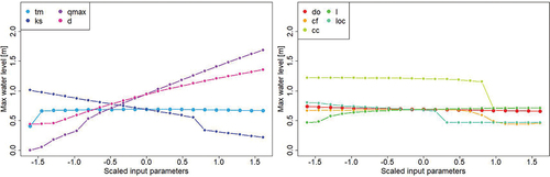
Table 3. Ranges and fixed values of the inputs used for the individual sensitivity analyses.

	ks [-]	qmax [m^3/s]	tm [s]	d [s]	do [s]	cf [m]	cc [m]	l [m]	loc [m]
Min	10	200	900	4500	0	2.6	7.5	1	2200
Max	20	500	3600	14,400	10,800	7.4	7.7	800	2800
Fixed value	15	300	2700	7200	5400	5	7.6	400	2500

Here we only present the results for the output P7. The trend is almost the same for the 3 other outputs. The Figure 5 shows the maximum water level in P7 as a function of scaled input parameters. On the left side, the hydraulic parameters are represented and we can see that they have much more influence than the breach parameters (on the right side). The flow (qmax), the duration (d) and the Strickler coefficient (ks) have a strong influence on the output contrary to the time to peak (tm). Regarding the breach parameters, the opening duration (do) seems to have no influence and the other inputs are a little more influent. The control level of the breach (cc) is influent because if this parameter is too high, there is no breach, which explain the step in the figure.

Finally, as the breach parameters seems to have a low influence on the outputs, we decided to do two UQ and GSA using the methodology presented in 3: one with all inputs considered being uncertain and one only with breach parameters as uncertain inputs (do, l, cf, loc, and cc).

4.2. UQ & GSA considering all the inputs uncertain

As explained previously, from the learning basis of 200 simulations with 9 inputs and 4 outputs, 4 metamodels were built and validated. The validation criteria computed with the cross validation method are available in Table 4.

Table 4. Metamodels validation criteria.

Output	RMSE	MAE	Q^2
P7	0.228	0.154	0.851
P9	0.258	0.175	0.875
P18	0.260	0.186	0.850
P20	0.309	0.209	0.840

The quality criteria are good meaning that the metamodels well represent the model. Therefore, the metamodels will be used to make new simulations useful for UQ and GSA.

4.2.1. Uncertainty quantification

For the UQ, 1000 simulations considering all inputs being independent and 1000 others considering some inputs being dependent have been made. The Figure 6 represents the outputs distributions and Figure 7 shows the outputs empirical Cumulative Distribution Functions (eCDF). First, the outputs ranges approximately from 0 to 4 m with a maximum around 1 m. A few outliers are negative but they have no physical meaning, there are due to the metamodels errors. The values equal to 0 mean that there is no breach or the breach is too small which do not impact the water level in the floodplain. The outputs densities nearly follow log normal distributions and we note a different behaviour of the output P7 with respect to the 3 other outputs. The outputs distributions of the points P9, P18 and P20 show plateaus which do not exist at the point P7, located upstream and not far from the river (Figure 1). Then, we note a significant difference between the case where all inputs are independent (in red) and the one where they are not (in blue). The difference is especially pronounced in the tail distribution.

Figure 6. Maximum water level distributions at the 4 output points considering independent inputs (in red) or dependent inputs (in blue).

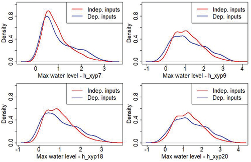
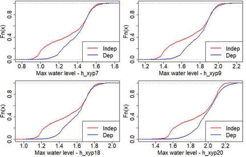
Figure 7. eCDFfor the maximum water level distributions at the 4 output points considering independent inputs (in red) or dependent inputs (in blue).

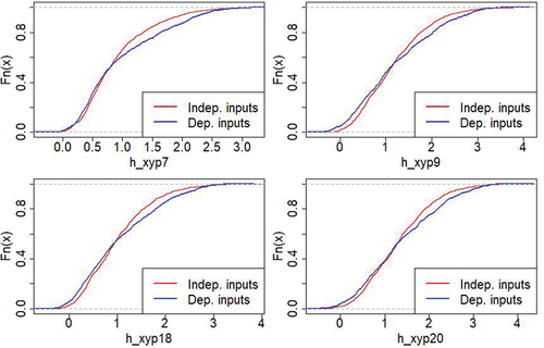
For example, for the output P7, 95% of the outputs are below 2.04 m if the inputs are considered being independent and 95% are below 2.36 m if some inputs are dependent. There is more than 30 cm of difference which is significant.

4.2.2. Global sensitivity analysis

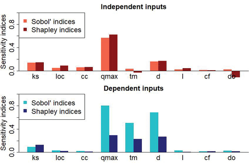
Two GSA have been made, one allowing to compute the first-order Sobol’ indices (left graph in Figure 8) and one to compute the Shapley indices (right graph in Figure 8). The Figure 8 illustrates the indices for all inputs contrary to Figure 9 which shows the indices only for the output P7. Theses graphs show.

• The behaviour of the 4 outputs is similar almost all considering the Sobol’ indices. With the Shapley indices, there are a little more differences but the parameters ranking remains the same;

• In case of dependent inputs or not and for both types of indices, the 5 breach parameters and ks have a very small influence on the outputs;

• Considering independent inputs, qmax has a strong influence and d is also influent. tm has no influence but when these three parameters are considered being dependent, they all have a strong influence;

• Regarding the output P7 and the case with dependent inputs, the ranking parameter is the same for both types of indices: the most influent inputs by order of importance are qmax, d, tm and ks;

Figure 8. 1st order Sobol’ indices (on the left) and Shapley indices (on the right) for the 9 uncertain inputs, considering independent inputs (circles) or dependent inputs (triangles). The indices are represented for the 4 outputs.

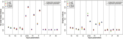
Figure 9. Comparison between the sensitivity indices (Sobol’ and Shapley) for the 9 inputs at the P7 output, considering independent inputs (upper graph) or not (lower graph).

4.3. UQ & GSA considering only the 5 breach parameters being uncertain

For this part, we built a new learning basis of 200 simulations only with 5 uncertain inputs. The hydraulic parameters are fixed (qmax = 400 m³/s, tm = 45 min, d = 2h30 and ks = 15) and the breach parameters are randomly sampled in the ranges presented in Table 2. We chose a small flow in order to see the breach effect on the outputs. In fact, if the flow is too high, the breach effect is negligible. Once the outputs computed, 4 new metamodels are built and validated. The validation criteria computed with the cross validation method are available in Table 5.

Table 5. Metamodels validation criteria.

Output	RMSE	MAE	Q^2
P7	0.103	0.068	0.892
P9	0.098	0.064	0.831
P18	0.102	0.07	0.822
P20	0.098	0.062	0.826

The validation criteria are good and similar to the ones calculated in part 4.2, meaning that the metamodels well represent the model. Thus, they will be used to make new simulations useful for the following UQ and GSA.

4.3.1. Uncertainty quantification

Using the distributions presented in Table 2 and the metamodels previsouly built, two datasets with 1000 simulations each, have been made. The first one contains only independent inputs and for the second one, some breach parameters are dependent (cf. copulas in Table 2). The Figures 10 and 11 shows the outputs distributions and eCDF.

Figure 10. Maximum water level distributions at the 4 output points considering independent inputs (in red) or dependent inputs (in blue).

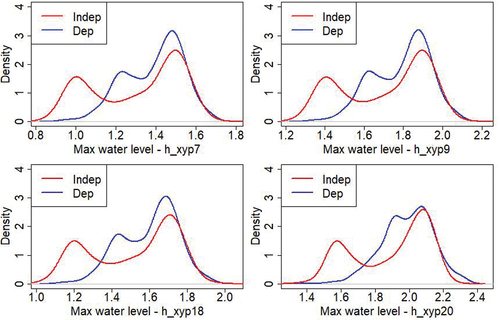
Figure 11. eCDF for the maximum water level distributions at the 4 output points considering independent inputs (in red) or dependent inputs (in blue).

In this case, the variation range is smaller than previsouly. In fact, the breach parameters are less influent than the hydraulic ones. The difference between the maximum outputs and the minimum outputs is around 1 m here and around 4 m in the case with 9 uncertain inputs. All outputs distributions present two peaks, in the case of independent inputs or not. The outputs P7, P9 and P18 show similar distributions contrary to P20. Once again, we note a significant difference between the case where all inputs are independent (in red) and the one where they are not (in blue). Here the difference is especially marked for low output values. The difference in the tail distribution is less obvious.

For instance, considering the output P7, 95% of the outputs are below 1.58 m if the inputs are considered independent and 95% are below 1.59 m if some inputs are dependent, which is insignificant (n.b. 20% are below 1.02 m with independent inputs, and below 1.24 with some dependent inputs).

4.3.2. Global sensitivity analysis

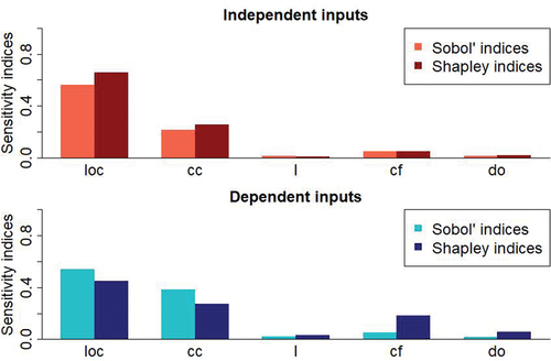
The same types of GSA than previsously have been made with the uncertain breach parameters (Sobol’ indices for all outputs on the left graph in Figure 8 and Shapley indices for all outputs on the right graph in Figure 12). The Figure 13 shows the indices only for the output P7. The findings from these graphs are;

• The behaviour of the 4 outputs is similar almost all considering the case with independent inputs and the Sobol’ indices. With the Shapley indices, there are a little more differences but the parameters ranking remains the same;

• Regarding the Sobol’ indices, only loc and cc seem to have an influence on the outputs but regarding the Shapley indices, also cf and do seem to be influent;

• The ranking parameter is always the same, regarding the type of indices and the case with independent inputs or not. The most influent inputs by order of importance are loc, cc, cf, do and l;

• There are a few differences between the cases with independent inputs or not. The only significant difference is for the parameter cf. It seems non influent regarding the independent case and the Sobol’ indices but regarding the Shapley indices in case of dependent inputs, it seems to have more influence. For instance for the output P9, which is downstream and close to the river, cf has as much influence as cc.

Figure 12. 1st order Sobol’ indices (on the left) and Shapley indices (on the right) for the breach uncertain parameters considering independent inputs (circles) or dependent inputs (triangles). The indices are represented for the 4 outputs.

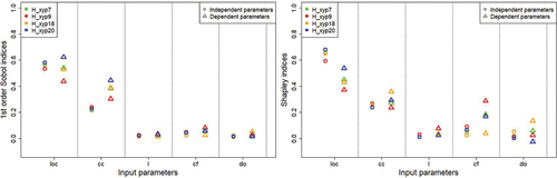
Figure 13. Comparison between the sensitivity indices (Sobol’ and Shapley) for the 5 breach parameters at the P7 output, considering independent inputs (upper graph) or not (lower graph).

5. Discussion

In this study, we simulated relatively low flows to see the breach effect on the outputs. In fact, if the flow is too high, the water passes widely over the dyke and the floodplain is inundated in case of dyke breach or not. It is why we made a second uncertainty analysis with only breach parameters. In a real case of application, extreme floods will be simulated.

Regarding the hydrograph parameters, the maximum flow (qmax) has a strong effect on the outputs and if the 3 hydrograph parameters are considered being dependent, they all have a major effect. It shows that the dependence between hydrograph parameters should not be neglected.

Regarding the breach parameters, the breach location (loc) and the control level (cc) have an important effect which seems normal in this simple case study. If the water level does not reach the control level, there is no breach and if the breach is located upstream (low loc) the water level reach faster the control level than if the breach centre is located downstream (high loc). For the breach dimensions, the parameters (l and cf) seem to have no effet or very few. Maybe with higher ranges and in a real case of application, they will be more influent.

In the part 4.3 where only breach parameters are considered, the differences between the case with independent inputs and the other one are more evident than in the part 4.2 (with all parameters considered) but the variation ranges are lower. We can imagine that in a real case of application, the differences will be higher which implies to take into account the dependence between inputs in future studies.

In both cases (parts 4.2 and 4.3), the sum of Sobol’ indices is much higher than 1 which not allows to estimate the share of variance of the output explained by each input, contrary to the sum of Shapley indices which is equal to 1. Therefore, if the objective is only to rank parameters, the Sobol’ indices can be used as the ranking is the same than the one with Shapley indices. Otherwise, to explain the share of variance of the output of one parameter, the Shapley indices are more suitable.

6. Conclusions and perspectives

In this work intended to provide a methodology to evaluate the effects of the dependence consideration between input parameters on the outputs, we chose to use a very simple case of application and to focus on hydraulic and breach parameters. After a first statistical analysis of input parameters (analyses of parameters probability distributions and dependences through copulas), we launched 200 simulations with the coupling tool Funz/TELEMAC-2D. Then kriging metamodels were built to make more simulations with low computational time. Finally, UQ and GSA were processed using the metamodels and considering independent inputs or not. We studied two cases, one with all the inputs (9 inputs) considered being uncertain and one with only breach parameters considered being uncertain.

Regarding the UQ, the output distribution is not the same with independent inputs or not. In case of 9 uncertain inputs the tail distribution differs. When some inputs are considered being dependent, the probability of exceeding some extreme values is higher than to the one with independent inputs. It confirms that the dependence should not be neglected in UQ studies. The differences are also visible in case of uncertain breach parameters but in all the distribution and not only in the tail. Finally, the output distribution is more reduced with only uncertain breach parameters than with uncertain breach and hydraulic parameters.

Regarding the GSA, two methods were tested, one allowing to calculate the Sobol’ first order sensitivity indices and one to compute the Shapley indices. Both show that when hydrograph parameters are considered being dependent, the 3 hydrograph parameters have a strong influence on the outputs contrary to the case with independent parameters. When only breach parameters are considered, the differences between the cases with independent or dependent inputs are less significant but there are. Finally, even if the ranking parameter is the same with Sobol’ first order and Shapley indices, the Sobol’ first order indices, in case of dependent inputs, do not allow to directly estimate the share of variance of the output due to each input, contrary to the Shapley indices.

In a near future, this methodology will be applied to the large 2D-model of the Loire river between Gien and Orleans. First this method will be just applied using the same parameters than in the current study and simulating breaches where historical breaches are known. Later we would like to improve some points: take into account the hydrographs shapes and not only use triangular hydrographs as input, integrate dykes fragility curves as model input because the breaches locations are deeply uncertain and consider over types of breaches and not only breaches by overflow.

Acknowledgments

We would like to thank Jérémy Rohmer from BRGM who provided the R-codes to compute the first-order Sobol’ sensitivity indices and Yann Richet from IRSN for building the coupling tool Funz/TELEMAC-2D.

Disclosure statement

No potential conflict of interest was reported by the author(s).

Data availability statement

The data that support the findings of this study are openly available in:

• the TELEMAC-2D “examples” for the simplified 2D model of inundation (telemac2d\breach) in http://www.opentelemac.org/index.php/component/jdownloads/summary/45-releases/1412-telemac-mascaret-v7p2r0-examples?Itemid=0;

• the “Banque Hydro” for the dataset of the Loire River (flow data at the station “La Loire à Gien” – K4180010) in http://www.hydro.eaufrance.fr/.

References

- Apel, H., Merz, B., & Thieken, A. H. (2008). Quantification of uncertainties in flood risk assessments. International Journal of River Basin Management, 6(2), 1–13. https://doi.org/10.1080/15715124.2008.9635344
- Bacchi, V., Duluc, C.-M., Bardet, L., Bertrand, N., & Rebour, V. (2018). Feedback from uncertainties propagation research projects conducted in different hydraulic fields: Outcomes for engineering projects and nuclear safety assessment. In Advances in hydroinformatics (pp. 221–241). Springer.
- Bacchi, V., Richet, Y., Bertrand, N., Moiriat, D., & Duluc, C., (2018). Beyond a sensitivity study of levee-breach geometry using an inversion algorithm: Application to a simplified river case., Conference CMWR 2018: Computational Methods in Water Resources XXII, Saint-Malo, France, 4–7 June 2018
- Balistrocchi, M., Ranzi, R., & Bacchi, B. (2014). Multivariate statistical analysis of flood variables by copulas: Two Italian case studies (pp. 12). Conference Paper: 3rd IAHR Europe Congress.
- Bertrand, N., Liquet, M., Moiriat, D., Bardet, L., Duluc, CM.et al (2018) Uncertainties of a 1D hydraulic Model with levee breaches: The benchmark Garonne. In: Gourbesville P., Cunge J., and Caignaert G. (eds) Advances in Hydroinformatics. Springer Water. Springer, Singapore
- Da Veiga, S., Wahl, F., & Gamboa, F. (2009, November). Local polynomial estimation for sensitivity analysis on models with correlated inputs. Technometrics, 51(4), 452–463. https://doi.org/10.1198/TECH.2009.08124.
- Domeneghetti, A., Vorogushyn, S., Castellarin, A., Merz, B., & Brath, A. (2013, August). Probabilistic flood hazard mapping: Effects of uncertain boundary conditions. Hydrology and Earth System Sciences, 17(8), 3127–3140. https://doi.org/10.5194/hess-17-3127-2013.
- DREAL Centre. (2011). Étude de dangers des digues de classe A de la Loire moyenne – Étude des brèches du val d’Orléans (code C4) – Annexe – Fiches de brèches.
- Dupuy, D., Helbert, C., & Franco, J. (2015). DiceDesign and DiceEval: Two R packages for design and analysis of computer experiments. Journal of Statistical Software, 65(11), 1–38. https://doi.org/10.18637/jss.v065.i11.
- Fang, K.-T., Li, R., & Sudjianto, A. (2005). Design and modeling for computer experiments. CRC press.
- Gratiet, L. L., Marelli, S., & Sudret, B. (2016). Metamodel-based sensitivity analysis: Polynomial chaos expansions and Gaussian processes. arXiv preprint arXiv:1606.04273
- Hervouet, J. M., & Ata, R. (2017). User manual of opensource software TELEMAC-2D (Report). EDF-R&D. www.opentelemac.org
- Iooss, B., Janon, A., Pujol, G., Broto, B., Boumhaout, K., Da Veiga, S., Delage, T., Fruth, J., Gilquin, L., & Guillaume, J. (2020). Sensitivity: Global sensitivity analysis of model outputs. R package version 1.24.0. Package available in https://cran.r-project.org/package=sensitivity
- Iooss, B., Mahévas, S., Makowski, D., & Monod, H. (2013). Analyse de sensibilité et exploration de modèles : Application aux sciences de la nature et de l’environnement. Editions Quae.
- Iooss, B., & Prieur, C. (2018). Shapley effects for sensitivity analysis with dependent inputs: Comparisons with Sobol’ indices, numerical estimation and applications. International Journal for Uncertainty Quantification, 39.
- Jacques, J., Lavergne, C., & Devictor, N. (2006, October). Sensitivity analysis in presence of model uncertainty and correlated inputs. Reliability Engineering & System Safety, 91(10–11), 1126–1134. https://doi.org/10.1016/j.ress.2005.11.047.
- The issue number is 76. The complete reference is: Korswagen, P. A., Jonkman, S. N., & Terwel, K. C. (2019). The issue number is 76. The complete reference is. Structural Safety, 76(june 2019), pp 135–148 https://doi.org/10.1016/j.strusafe.2018.08.001.
- Li, C., & Mahadevan, S. (2016). An efficient modularized sample-based method to estimate the first order Sobol׳ index. Reliability Engineering & System Safety, 153(September 2016), pp 110–121 https://doi.org/10.1016/j.ress.2016.04.012.
- Li, C., & Mahadevan, S. (2016, September). An efficient modularized sample-based method to estimate the first-order Sobol׳ index. Reliability Engineering & System Safety, 153, 110–121. https://doi.org/10.1016/j.ress.2016.04.012.
- Mara, T. A., Tarantola, S., & Annoni, P. (2015). Non-parametric methods for global sensitivity analysis of model output with dependent inputs. Environmental Modelling & Software, 72(2015), pp 173–183.
- Marrel, A., Iooss, B., Van Dorpe, F., & Volkova, E. (2008). An efficient methodology for modeling complex computer codes with Gaussian processes. Computational Statistics & Data Analysis, 52(10), 4731–4744. https://doi.org/10.1016/j.csda.2008.03.026.
- Mazo, G. (2014). Construction et estimation de copules en grande dimension. PhD Thesis, Université de Grenoble PhD Thesis
- McKay, M. D. (1995). Evaluating prediction uncertainty. Nuclear Regulatory Commission.
- McRae, G. J., Tilden, J. W., & Seinfeld, J. H. (1982). Global sensitivity analysis – A computational implementation of the Fourier amplitude sensitivity test (FAST). Computers & Chemical Engineering, 6(1), 15–25. https://doi.org/10.1016/0098-1354(82)80003-3.
- Nagler, T., Schepsmeier, U., Stoeber, J., Brechmann, E. C., Graeler, B., & Erhardt, T. (2019). VineCopula: Statistical inference of Vine Copulas. R package version 2.3.0. Package available in https://cran.r-project.org/package=VineCopula
- Nelsen, R. B. (2007). An introduction to copulas. Springer Science & Business Media.
- Owen, A. B., & Prieur, C. (2016, October). On Shapley value for measuring importance of dependent inputs. arXiv:1610.02080 [Math, Stat] [ Online]. Retrieved February 13, 2019, from http://arxiv.org/abs/1610.02080.
- Owen, A. B. (2014, janv). Sobol’ indices and Shapley value. SIAM/ASA Journal on Uncertainty Quantification, 2(1), 245–251. https://doi.org/10.1137/130936233.
- Pheulpin, L., Bacchi, V., and Bertrand, N. (2019). Analyse de sensibilité des paramètres de rupture des digues : Application au cas de la Garonne. Conference Digues Maritimes et Fluviales de Protection contre les Inondations, Digues 2019, Aix-en-Provence, France. pp. Art N°8. https://doi.org/10.5281/zenodo.2530017.
- Pheulpin, L., Bacchi, V., & Bertrand, N. (2020). Comparison between two hydraulic models (1D and 2D) of the Garonne River: Application to uncertainty propagations and sensitivity analyses of levee breach parameters. In Advances in hydroinformatics (pp. 991–1007). Springer.
- Ratto M, Tarantola S, Saltelli A, Young PC.et al Accelerated estimation of sensitivity indices using state dependent parametermodels. In: Hanson KM, and Hemez FM, editors, Sensitivity analysis of model output, Proceedings of the 4th international conference on sensitivity analysis of model output (SAMO 2004). Santa Fe, New Mexico; March 8–11 2004. p. 61–70.
- Richet, Y., & Bacchi, V. (2019). Inversion algorithm for civil flood defense optimization: Application to two-dimensional numerical model of the Garonne River in France. Frontiers in Environmental Science, 7, 160. https://doi.org/10.3389/fenvs.2019.00160.
- Roustant, O., Ginsbourger, D., & Deville, Y. (2012). DiceKriging, DiceOptim: Two R packages for the analysis of computer experiments by kriging-based metamodeling and optimization. Journal of Statistical Software, 51(1), 1–55. https://doi.org/10.18637/jss.v051.i01.
- Saltelli, A., Ratto, M., Andres, T., Campolongo, F., Cariboni, J., Gatelli, D., Saisana, M., & Tarantola, S. (2008). Global sensitivity analysis: The primer. John Wiley & Sons.
- Saltelli, A., Tarantola, S., Campolongo, F., & Ratto, M. (2004). Sensitivity analysis in practice: A guide to assessing scientific models. John Wiley & Sons.
- Saltelli, A. (2002). Making best use of model evaluations to compute sensitivity indices. Computer Physics Communications, 145(2), 280–297. https://doi.org/10.1016/S0010-4655(02)00280-1.
- Sanyal, J. (2017, juill). Uncertainty in levee heights and its effect on the spatial pattern of flood hazard in a floodplain. Hydrological Sciences Journal, 62(9), 1483–1498. https://doi.org/10.1080/02626667.2017.1334887.
- Song, E., Nelson, B., and Staum, J. (2016). Shapley effects for global sensitivity analysis: Theory and computation, SIAM/ASA. Journal on Uncertainty Quantification, 4(1), 1060–1083.
- Vorogushyn, S., Apel, H., & Merz, B. (2011, January). The impact of the uncertainty of dike breach development time on flood hazard. Physics and Chemistry of the Earth, Parts A/B/C, 36(7–8), 319–323. https://doi.org/10.1016/j.pce.2011.01.005.
- Wahl, T. L. (2004). Uncertainty of predictions of embankment dam breach parameters. Journal of Hydraulic Engineering, 130(5), 389–397. https://doi.org/10.1061/(ASCE)0733-9429(2004)130:5(389).