Operational hydrometeorological forecasting on the Rhône River in France: moving toward a seamless probabilistic approach

ABSTRACT

Compagnie Nationale du Rhône (CNR) has operated the Rhône River since 1934 according to three core missions – hydropower generation, inland navigation and irrigation – using 19 run of-river multi-purpose hydropower schemes. To ensure hydraulic safety and optimise hydro power production and commercialisation, CNR developed a range of hydrometeorological forecasting tools, currently run every day in real time by CNR forecasters. The first is an hourly deterministic tool, giving forecasts up to the next 4 days. This tool does not allow quantification of uncertainties, which is a key issue to improve forecasts and take better operational decisions. At the same time, national meteorological centres provide ensemble meteorological forecasts, and thus information about uncertainty. Therefore, CNR is developing a chain of ensemble forecasting tools based on ensemble meteorological forecasts and various post-processing methods. These tools provide hourly/daily hydrological forecasts up to the next 4/12 days. The operational use of such a probabilistic forecasting chain is intended to facilitate decision-making processes. All these tools have been designed to leave large room for human expertise. This paper presents the tools described above, but also their interaction with human forecasters as well as the first attempts to link them together to add consistency between the different forecast types.

RESUME

Compagnie Nationale du Rhône (CNR) pilote la concession du Rhône français depuis 1934, et développe les activités sur le fleuve selon trois missions principales – la génération d’hydroélectricité, la navigation sur le fleuve, et l’irrigation des terres agricoles – grâce à 19 aménagements hydroélectriques fonctionnant au fil de l’eau. Afin de garantir la sécurité hydraulique, et d’optimiser la production d’hydroélectricité et sa commercialisation, CNR a développé un panel d’outils de prévisions hydrométéorologiques, proposant des prévisions météorologiques, des prévisions hydrologiques ou encore des prévisions de production et leur optimisation. Ces outils sont utilisés quotidiennement par des prévisionnistes CNR, en complément de leur expertise, afin d’éditer des bulletins de situation hydrologique à destination de divers services, dont les gestionnaires d’aménagements. Un premier outil propose des prévisions horaires déterministes sur les 4 prochains jours. Cet outil ne permet pas de prendre en compte les multiples incertitudes provenant de différentes sources. Quantifier ces incertitudes est l’une des clés d’amélioration des prévisions. En parallèle, les centres météorologiques nationaux et internationaux fournissent des prévisions météorologiques d’ensemble, basées sur plusieurs scénarios équiprobables, et permettant ainsi d’obtenir des informations sur les incertitudes météorologiques. En conséquence, CNR développe une chaine d’outils de prévisions d’ensemble, basés sur ces prévisions météorologiques, de multiples modèles et différentes méthodes de post-traitement. Avec cette information sur les incertitudes, l’utilisation opérationnelle de cette chaine tend à faciliter le processus de décision (gestion des inondations, vente d’énergie, etc.). Le but de ce papier est de présenter l’ensemble des outils opérationnels utilisés afin d’établir des prévisions quotidiennes prenant en compte les incertitudes. L’organisation de CNR autour de ces outils ainsi que l’utilisation qu’en font les prévisionnistes sera également détaillée. Enfin, ce papier présentera les premières tentatives de mise en cohérence des prévisions fournies par ces différentes chaines d’outils.

KEYWORDS:

• Hydrometeorological forecasts
• operational tools
• hydropower production optimisation
• probabilistic forecasting

MOTS CLES:

• Prévisions hydrométéorologiques
• outils opérationnels
• optimisation de la production hydroélectrique
• prévisions d’ensemble

1. Introduction

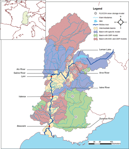
In 1934 Compagnie Nationale du Rhône (CNR) received from the French government the concession of the Rhône River to develop and operate the river according to three core missions: hydropower generation, inland navigation and irrigation. Over the past 85 years, CNR has designed and built 19 run-of-river multi-purpose hydropower schemes with a total installed capacity of 3021 MW. The Rhône River is a major river in France (approx. 95,000 km² and 1600 m³/s at Beaucaire – downstream Rhône River) and is subject to various climatic influences, as well as human activities (see Figure 1 for the area covered by the Rhône River basin).

Figure 1. Map of the Rhône River basin divided into 48 sub-catchments. Hydrometeorological models set up by CNR in each sub-basin for the short-term tools are presented in colour.

Like many operators worldwide, whether for flood warning purposes from local (Addor et al., 2011) to continental scales (Thielen et al., 2009a), or for hydropower production (Desaint et al., 2009), CNR developed its own streamflow forecasting system (Bompart et al., 2008). This system is composed of various hydrometeorological forecasting tools, adapted to different stakes: production valorisation, maintenance scheduling, support for operators (floods and low flows), optimisation for the electricity balancing market, etc.

Historically, the first tool to be set up was an hourly deterministic hydrometeorological forecasting chain, dedicated to short-term forecasts (up to 4 days ahead). This tool, based on meteorological forecasts subject to human expertise, provides an estimation of the Rhône River tributaries’ streamflow. It makes the most of all available hydrological and meteorological knowledge to produce the most accurate and informative predictions possible, as advocated by Pagano et al. (2014). This historical tool, of primary importance for CNR, is used daily by forecasters, and is essential for hydraulic safety as well as hydropower production optimisation.

Quantifying uncertainties coming from various sources (observations, meteorology, modelling, hydraulic propagation, etc.) is a key issue to improve forecasts and to provide better estimations of extreme events. Today several national and international meteorological centres provide ensemble meteorological forecasts: as an example, the International Grand Global Ensemble (TIGGE; Bougeault et al., 2010) project gathers access to ensemble predictions from more than 10 global numerical weather prediction (NWP) centres. Based on several equiprobable scenarios, the ensemble forecasts provide information on meteorological uncertainty. Those meteorological scenarios can be used as input to streamflow forecasting tools to propagate meteorological uncertainties to discharge estimations. During the last 15 years, probabilistic streamflow forecasting arising from meteorological ensembles has progressively evolved from a research field (Cloke & Pappenberger, 2009) to an operational reality (Bennett et al., 2017; Moulin et al., 2019), even if a large variety of approaches and methods can lead to ensemble predictions (Troin et al., 2021).

CNR is also developing a chain of ensemble forecasting tools, based on ensemble meteorological forecasts and various post-processing methods. These probabilistic tools are developed with the objective to meet the specific needs associated to different forecasting horizons: short-term predictions (up to 4 days ahead) for flood warning and day-ahead energy sales; mid-term forecasts (up to 14 days ahead) for maintenance scheduling and control reserve availability sales for the electricity network; and seasonal tendencies (up to 3 months ahead) for long-term energy sales. Because prediction uncertainties increase with forecasting horizons, the need to jointly use several probabilistic approaches with spatial and temporal features adapted to each target horizon is crucial to achieve the best predictability without omitting information on uncertainties (Demargne et al., 2014; Thielen et al., 2009b). The simultaneous use of several tools can result in non-coherent predictions at the juncture of specific time horizons, and thus cause discontinuities in the resulting overall forecast. Therefore, seamless approaches are developed with the aim to keep forecasts coherent along the temporal scale. Seamless forecasting chains are now commonly used in other domains such as solar (photovoltaic) power predictions (e.g. Carriere et al., 2020), where operational needs can range from very short-term horizons (1 minute ahead) to several days, forcing predictions to rely on various meteorological sources (sky imagers, satellites, NWP) and combining them with statistical approaches (Lorenz et al., 2014). Seamless approaches are also used for hydrological predictions, as illustrated by Wetterhall and Di Giuseppe (2018).

In this way, three probabilistic hydrometeorological tools have been developed at CNR. The probabilistic equivalent of the historical deterministic chain provides an ensemble of 51 hourly hydrological scenarios for the short-term horizon, using meteorological forecasts provided by the European Centre for Medium-Range Weather Forecasts (ECMWF) and two hydrological models. A second tool, dedicated to mid-term tendencies, provides an ensemble of 51 daily hydrological scenarios, considering only the meteorological uncertainty, up to 14 days ahead. A last tool provides seasonal predictions of production, up to 3 months ahead. Thus, in the end, four tools (one deterministic, three probabilistic) are used by CNR forecasters. Thanks to their information content regarding uncertainties, the operational use of these forecasting chains is intended to facilitate decision-making processes (operations during floods, energy sales, etc.), even if interpretating and communicating on probabilistic forecasts without omitting essential information always represents an operational challenge (Demeritt et al., 2010).

Drawing on its own experience acquired for many years, reinforced by the large consensus existing on the added value of human expertise on streamflow forecasting (Berthet et al., 2019; Celié et al., 2019; Moulin et al., 2019), CNR designed all its operational tools leaving a large amount of room for human expertise. However, adding expertise to a chain of three successive probabilistic forecasts is not as simple as it could be for one deterministic prediction – first, because the tools should provide mutually consistent forecasts to avoid duplicated expertise on each tool; and, second, because probabilistic streamflow forecasts should be post-processed to correct biases and are subject to spatial and temporal coherence reconstruction (Bellier et al., 2018; 2021). Thus, adding expertise while keeping this coherence represents a major operational challenge (Berthet et al., 2019).

The aim of this paper is to present the different tools described above, their interaction, and their use with the forecaster’s expertise to provide operational forecasts. Section 2 presents in detail the area operated by CNR. Section 3 focuses on the deterministic hydrometeorological chains, whereas Section 4 focuses on the probabilistic hydrometeorological chain. Section 5 deals with the interaction between these tools and CNR forecasters, as well as the first attempts to link these tools together. Section 6 then concludes the paper.

2. Area operated by CNR

CNR operates hydroelectric facilities along the French Rhône River. Figure 1 provides a map of the related catchment, as well as the main tributaries where hydrological forecasts are produced. The division of the Rhône River basin into multiple sub-basins depends on the tool used for the forecast.

The finer breakdown provides 53 sub-catchments. It is mainly used for the meteorological forecasting at hourly time steps (see Section 3.3.1 about the OPALE tool). A cut in 48 sub-catchments is used for the hydrological forecasting at an hourly time step (Section 3.3.2 about the PHARE tool). The difference between these two cuts is the Durance catchment (at the bottom right in Figure 1), divided into six sub-catchments for the meteorological forecast, and into one catchment for the hydrological forecast. This is due to the high anthropogenic influence on this basin, as well as the poor hydrological data quality associated to some stations. Figure 1 shows this division, into 48 sub-catchments. These two cuts are used for both the deterministic (Section 3) and the probabilistic (Section 4.1) hourly forecasts (short term).

Another breakdown into 24 sub-catchments is used for the probabilistic daily hydrometeorological forecasting tool presented in Section 4.2 (mid-term; see the map on the left of Figure 9), which demands less accuracy. Finally, the last tool giving seasonal tendencies (Section 4.3) considers a division into only two zones: the Upper Rhône River and the Lower Rhône River (above and below the city of Lyon).

3. Deterministic hydrometeorological chain

CNR’s deterministic hydrometeorological chain (Bompart et al., 2008) is designed for short-term forecasting (lead times from day D to day D + 4, hourly time step), to ensure hydraulic safety and to optimise hydropower production. For the hydropower production selling in markets, the forecast at day D + 1 is the most important.

3.1. Objectives

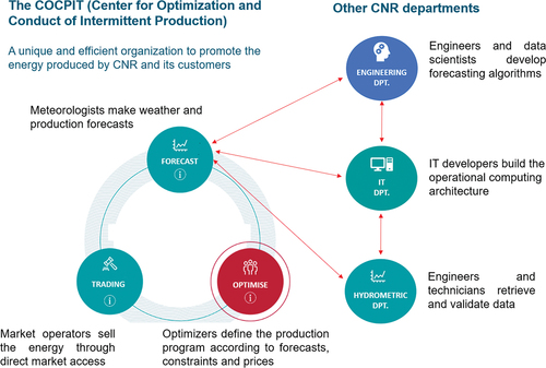
Since the liberalisation of the European energy market, which began in France in 1999 following EU Directive 96/92/EC, CNR has organised its tools to efficiently manage its production assets. Different internal players interact with each other to ensure hydraulic safety while optimising electricity production in a reactive manner (see Figure 2). One of the main challenges is the daily creation of the next day’s production program to optimise the selling of production on the energy wholesale market. This production program is based on a single scenario that represents the best CNR forecast – at the forecasting time – for the next day. Upstream of a complex and precise operational process is the estimation of the hydrological resources of the river and its tributaries. This task is carried out by the Intermittent Production Management Centre, which is particularly in charge of hydrometeorological forecasting. CNR relies on hydrometeorological forecasters to ensure operational activity, while a team of the Engineering Department oversees the development of specialised forecasting tools. Expertise plays an important and essential part in the forecasting process at CNR (Celié et al., 2019).

Figure 2. CNR organisation around the forecasting tools.

3.2. Data

Data used in this hydrometeorological chain include observed and forecasted meteorological data as well as observed discharge data. Gridded information is aggregated at the spatial scale of the 53 sub-catchments of the Rhône River (see Figure 1).

3.2.1. Observations

Six-hourly gridded meteorological observations for precipitation and temperature, as well as 15-minute time step rainfall estimated by meteorological radars, are provided by Météo-France.

Discharge data are collected through the CNR hydrological network, which gathers about 300 measurement points on the Rhône River and its main tributaries. Partnerships with other data producers allow CNR to complete its network (approx. 140 stations from CNR and 160 stations from partnerships).

3.2.2. Forecasts

Hourly gridded precipitation and temperature forecasts are provided by Météo-France. These forecasts are re-processed by CNR forecasters, as detailed in Section 3.3.1.

The altitude associated to the equivalent potential temperature at 1°C (θ’w) is also provided by Météo-France as a gridded forecast. It is used as a guess of the rain–snow limit, which is the altitude at which snow mostly turns into rain. The θ’w temperature is the temperature a parcel of air would have if (a) it was lifted until it became saturated; (b) all water vapour was condensed out, and (c) it was returned adiabatically (i.e. without transfer of heat or mass) to a pressure of 1000 millibars.

3.3. Tools

The deterministic hydrometeorological chain is made of various interconnected tools (see Figure 3). They are presented above. The meteorological tool applies to 53 sub-catchments, whereas the hydrological tool applies to 48 sub-catchments (Durance River basin is considered as one basin instead of six sub-basins in the hydrological modelling). The 48 sub-catchments are distributed as follows:

Figure 3. Schematic description of the short-term deterministic forecasting chain.

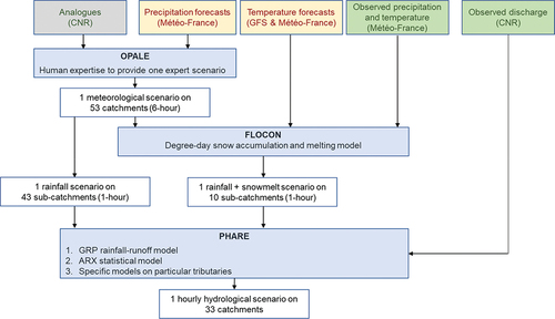
• Twenty-seven sub-basins have one or two calibrated hydrological models. This group of basins is coloured in either green or red in Figure 1;

• Six sub-basins, with a strong anthropogenic influence, have a specific model. Depending on the catchment, this model could be a mix between propagation and statistical models; it could also use energy prices as explanatory variables, or forecasts from other services operating the river. These models do not provide optimised forecasts. For this reason, CNR forecasters manually define the forecast using the result of these models as a first guess. This group of basins is coloured in purple in Figure 1;

• Eleven small tributaries do not have a model and four sub-basins are intermediate watersheds on the Rhône River. For the estimation of flows, the 11 small tributaries without hydrological models are included into those four intermediate watersheds. An estimation of the flow from these intermediate watersheds is obtained using a weighting average of flows from the main contributing tributaries. This group of basins (4 + 11) is coloured in beige in Figure 1.

In this paper, the hydrological modelling details will focus on the processes set up for the 27 sub-basins with one or two calibrated models.

3.3.1. Meteorological step: the OPALE tool

The OPALE© software is dedicated to meteorological expertise and forecasting on the 53 sub-catchments. The strategy adopted by CNR in terms of rainfall forecasting consists in having different sources of information, comparing them, adding human expertise and finally building up an “expert rainfall scenario”. CNR has several distinct and complementary sources of quantitative precipitation forecasts on 53 catchments (denoted QPF, precipitations aggregated at a sub-catchment’s scale), at a 6-hourly time step:

1. Precipitation with expertise, provided by the Météo-France regional forecast centre;

2. An analogue model (Ben Daoud et al., 2016; Bontron, 2004; Obled et al., 2002), based on the selection of past situations that are similar to the ongoing situation, in terms of synoptic variables. The selection of analogue situations is done stepwise, each step selecting a specific number of situations following a specific predictor. The first predictor is 2-m temperature, allowing a sorting by season. The second predictor is geopotential height at 500 and 1000 hPa. The final predictor is relative humidity at 850 hPa. The closest analogue situation at this step is kept, in order to obtain only one precipitation forecast at the end of this method;

3. Raw gridded precipitation outputs from various NWP models, such as AROME (Applications de la Recherche à l'Opérationnel à Méso-Echelle, Météo-France) and ARPEGE (Action de Recherche Petite Echelle Grande Echelle, Météo-France) (Météo-France), GFS (Global Forecast System, NWS) or IFS (Integrated Forecasting System, ECMWF and Météo-France) (ECMWF) (see Table 1 for the main models used by the forecasters).

   Table 1. Meteorological models.

   Model	Resolution
   GFS (NWS) National Weather Services	0.1°
   ARPEGE (Météo-France)	0.1°
   CEP Modèle du Centre Européen de Prévisions (ECMWF) European Centre for Medium-Range Weather Forecasts	0.1°
   ICON 2D and ICON (German Weather Service/Max Planck) Icosahedral Nonhydrostatic	2 and 7 km
   AROME (Météo-France)	0.01°
   EURO4 (MetOffice)	4 km
   IFS (ECMWF and Météo-France)	18 km

CNR forecasters gather the data from these three sources to provide forecasted precipitations and temperatures.

An internally developed degree-day snow accumulation and melting model, FLOCON, is run on 10 catchments influenced by snow (see Figure 1 for the related sub-basins). The forecasters construct their own expert scenario and alternative hypotheses for precipitations and snow parameters. To do that, they evaluate the rain–snow limit with other external sources (for example, webcams and collaborative sites such as www.infoclimat.fr). They also manually evaluate the snow stock from FLOCON, using satellite maps, as well as temperature forecasts by comparing them to various NWP models. For these basins, this step provides a rain/snow repartition as well as a snow stock and a snowmelt runoff.

The expert forecasted precipitation and temperature scenario is then used as input to CNR hydrological models in the hydrological tool PHARE (Section 3.3.2). For snowmelt-driven basins, the input precipitation is the sum of rainfall and snowmelt.

3.3.2. Hydrological step: the PHARE tool

PHARE is the tool dedicated to hydrological forecasting. Hydrological forecasting is performed on the main tributaries of the Rhône River and the four intermediate catchments. It uses as input the expert meteorological scenario imported from OPALE and disaggregated from the 6-hour time step to an hourly time step. The disaggregation consists in dividing the 6-hour accumulated precipitation by six and attributing the same value to each of the six resulting time steps. The second input is hourly observed discharge data since the last forecast. PHARE produces hourly time step hydrological forecasts for a maximum lead time at day D + 4. This forecast is updated at least 3 times a day.

Two types of models are implemented on most of the tributaries (the 27 in red or green in Figure 1). First, a fully statistical autoregressive-exogenous (ARX)-type model (Remesan and Mathew 2015) is calibrated on 21 sub-basins, over the 2008–2020 period. The calibration is done on high-flow events, which are selected in the calibration period. This model uses an index representing the soil humidity, called the index of previous precipitation (IPP), following Equation (1)(1) $IP{P}_t=IP{P}_{t-1}+K\ast P_{t-1}$(1) :

(1) $IP{P}_t=IP{P}_{t-1}+K\ast P_{t-1}$(1)

In Equation (1)(1) $IP{P}_t=IP{P}_{t-1}+K\ast P_{t-1}$(1) , K is a fixed coefficient and P represents precipitation.

A segmentation into flow ranges and IPP ranges is done, then regression equations are calibrated on each range. The particularity of this model is to use different equations depending on the range, so that a continuous high-flow event can use different equations. The equations use previous precipitation (6-hour time step) and previous flows (1-hour time step), as presented in Equation (2)(2) $Q_t=\hspace{0.17em}\alpha Q_{t-1}+\hspace{0.17em}\beta Q_{t-2}+\dots +\hspace{0.17em}\gamma P_{t-1}+\hspace{0.17em}\delta P_{t-2}+\dots$(2) :

(2) $Q_t=\hspace{0.17em}\alpha Q_{t-1}+\hspace{0.17em}\beta Q_{t-2}+\dots +\hspace{0.17em}\gamma P_{t-1}+\hspace{0.17em}\delta P_{t-2}+\dots$(2)

The number of previous flows and precipitation can vary following the range and the basin.

Second, a GRP (Modèle de Génie Rural Prévisionnel) model, which is a conceptual reservoir model developed by INRAE (Institut National de Recherche pour l'Agriculture et l'Environnement) (Berthet, 2010; Berthet et al., 2009), is calibrated over the 27 sub-basins. This model uses two reservoirs and needs three parameters that are calibrated using the continuous 2012–2020 period. The three parameters of the GRP model are:

• The adjustment factor of effective rainfall which contributes to finding a good water balance (by accounting for possible water exchange with underground (unitless, should be close to 1);

• The capacity of the routing store (in mm);

• The unit hydrogram (UH) time base used to account for the time lag between rainfall and streamflow (in hours).

When the GRP model is used for a forecast, all the state variables should be initialised. The first time, the model is run during 1 year before the forecast, using observed precipitation provided by Météo-France and observed discharge data. Then, for each subsequent forecast, an assimilation scheme updates the reservoir level at each step by comparing the simulated flow to the observed one. Consequently, the last level obtained (1 hour before the forecast) produces a simulated flow equal to the observed one.

On certain tributaries influenced by dams (Isère River, Ain River) or on large tributaries (Saône River), specific mixed modelling techniques combining hydraulic propagation and rainfall-runoff forecasts have been implemented. Regarding the Leman lake outflow, forecasts from Services Industriels de Genève (SIG) are taken into account. The results of these models are used as a first guess by CNR forecasters to create the final hydrological forecasts, based on their experience. The related basins are coloured in purple in Figure 1.

Lastly, the flow on the four intermediate watersheds on the Rhône River (including 11 small tributaries without models) is computed using a weighting average of flows on the main contributing tributaries (in beige in Figure 1). These different set-ups (ARX and/or GRP, specific models, intermediate watersheds) are indicated by colour in Figure 1.

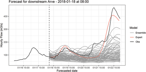
Like the meteorological step, the hydrological step involves human expertise. The different models, fed with different meteorological inputs, may result in a wide range of possible hydrological scenarios which are assessed by the forecaster to build the most probable scenario for each tributary (more details in Section 5). This final scenario, forming the deterministic reference forecast, will lastly be used as input to hydraulic propagation models (see Section 3.3.3). A result of the GRP model, the ARX model and the Expert model is provided in Figure 4 for the downstream Arve River, for a forecast at 9am on 18 January 2018.Figure 5

Figure 4. Example of results of the deterministic hydrological chain on the downstream Arve for 18January2018.

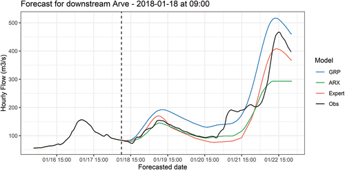
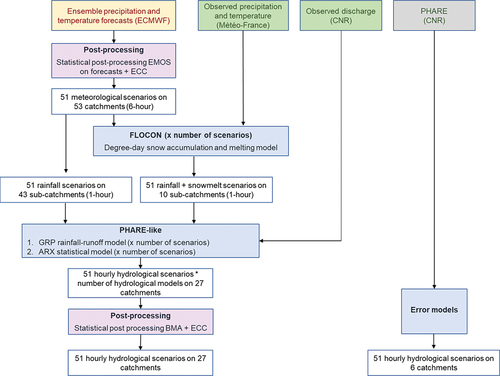
Figure 5. Schematic description of the short-term probabilistic forecasting chain.

3.3.3. Hydraulic propagation

Once validated, the forecasts on tributaries are imported into hydraulic models, which model the propagation of flows on the Rhône River. The water levels and hydroelectric production forecasts are thus computed for each hydropower development.

Depending on the hydraulic conditions, two kinds of models are considered:

• For discharges not exceeding the turbine capacity of the developments, only mean propagation times are considered. A high computation speed is necessary to optimise the power production scheduling thanks to the active storage capacity of the Rhône cascade (Piron et al., 2015). These propagation tools also integrate interfaces to perform this optimisation with respect to the operating constraints (water levels to be respected, admissible flow gradients, availability of turbines, etc.).

• For higher discharges, there is no need for optimisation (as the storage capacities are filled) and hydrograph deformations become sensible. We thus consider a one-dimensional looped-network hydraulic model with additional storage area (Grimaldi et al., 2014) covering the whole course of the Rhône River.

Once again, the human expertise is present in this hydraulic step (see Section 5).

4. Probabilistic hydrometeorological chains

Probabilistic forecasts provide information on uncertainties that is not found in a deterministic approach. Integrating this information leads to better decision-making, and thus improves the quality of governance (Ramos et al., 2013). Three probabilistic tools are introduced in this section, each developed for a specific lead time (short-, mid- and long-term). The mid- and long-term tools are already operationally used, whereas the short-term tool is still under development.

4.1. Short-term

Probabilistic meteorological forecasts have been provided by climate centres for several years. The ensemble approach allows us to quantify the uncertainty of weather models and to capture a part of climate variability. It is then possible to translate this uncertainty into hydrological forecasts. The developed tool post-processes ensemble meteorological and hydrological forecasts. Based on the PhD work of Bellier (2018), co-funded by CNR, it provides reliable spatially and temporally coherent hydrometeorological predictions. This tool is a probabilistic equivalent of OPALE + PHARE, providing hourly ensemble forecasts up to 4 days ahead. It has been under development since 2019, and a prototype version will be available to forecasters in 2022.

4.1.1. Data

The short-term forecasting chain relies on the use of precipitation and temperature forecasts from the Ensemble Prediction System (EPS; Molteni et al., 1996) provided daily by the ECMWF. CNR needs to produce forecasts at 8am CET. For this purpose, the run of 12am UTC (the day before the forecast) is used. Indeed, the run of 00UTC is not available on time for our forecasts, especially in summer (available at 9am CET time). Data consist in 51 scenarios of precipitation and temperature, available on a 0.25° x 0.25° grid and at a 6-hour time step. Each scenario is spatially aggregated over the 53 catchments. Other meteorological sources will be added in the future, such as forecasts provided by the Global Ensemble Forecast System (GEFS) model, from the National Centers for Environmental Prediction (NCEP) DOC/NOAA/NWS/NCEP/EMC. For now, the meteorological uncertainty is considered only through the EPS model, but using more than one NWP model will allow us to consider uncertainties associated with weather models. The observed data are the same as those considered for the deterministic forecasting chain: quantitative precipitation estimates, provided by Météo-France, and discharge data collected through the CNR hydrological network.

4.1.2. Methods

The methodology comprises various steps, and thus the tool is composed of different modules, following Figure 5. Ensemble forecasts available on a 6-hour time step in 53 basins are first post-processed using the ensemble model output statistics (EMOS; Gneiting et al., 2005) approach, which corrects the lack of reliability observed in the raw forecasts (an example is given in Figures 9 and 11 with the mid-term tool). The work of Bellier (2018), while confirming the dominant effect of streamflow post-processing on streamflow prediction performances as previously shown by Zalachori et al. (2012), have nonetheless proved the benefit of a two-step bias-correction methodology (post-processing of meteorological inputs + post-processing of streamflow forecasts) as compared to a single post-processing of discharge predictions only. The EMOS method is calibrated over a chosen period, where it compares ensemble forecasts to observations to fit a parametric distribution considering summary statistics from the ensemble. The calibration period depends on the post-processed variable. For precipitation, the height years before the year of the forecast are used. This number is reduced to the 4 previous years for temperature. To give an example, if a forecast is done in 2022, the 2014–2021 period will be used for precipitation and the 2018–2021 period will be used for temperature. These choices have been made after a sensibility study testing multiple calibration period configurations. It showed that updating the EMOS parameters using the most recent years improved the forecasts (not shown). Post-processed meteorological data are then re-ordered following an ensemble copula coupling approach (ECC; Schefzik et al., 2013; Bellier et al., 2017) to construct spatio-temporally coherent scenarios. At the end of this step, 51 meteorological scenarios are available.

These scenarios then serve as input to the FLOCON module for specific catchments where snow modelling is mandatory (the 10 sub-basins highlighted in Figure 1). Snowmelt outputs from FLOCON, calculated at a 6-hour time step (or post-processed precipitation if FLOCON is not used), are then temporally disaggregated at the hourly time step, as is done in the deterministic tool. They then serve as input to hydrological models, using an ARX statistical model, a GRP rainfall-runoff model, or both, depending on the catchment (see Figure 1). The same calibrated models are used for both the deterministic short-term tool (PHARE) and this tool. As for the deterministic PHARE platform, an assimilation scheme since the last forecast is also set up for the GRP modelling. At the end of this step, 51 or 102 hydrological scenarios are available on each sub-basin, depending on the number of available hydrological models.

The hydrological outputs are finally post-processed using Bayesian model averaging (BMA; Raftery et al., 2005), which fits a mixture density as predictive distribution, associating a kernel function to each ensemble member. This method is calibrated using the 4 years before the forecast. An ECC approach, adapted as proposed by Bellier et al. (2018) to deal with the specificities of hydrological data, is applied on the hydrological scenarios. Using this method, it is possible to choose the number of output hydrological scenarios, independently of the number of scenarios used as inputs. For our purposes, the selected number is 51. This finalises the process to provide 51 hourly hydrological scenarios for all the 27 sub-basins.

Six specific catchments, where mixed modelling techniques are used in PHARE, cannot be modelled using only rainfall-runoff approaches because of anthropogenic influences. For these catchments, error models have been calibrated to dress the PHARE forecast with uncertainties, transforming the deterministic forecast into a 51-member ensemble forecast. Adding human expertise to the probabilistic forecasts is not possible in the current tool, but internal studies will begin to provide this functionality.

Figure 6 provides an example of post-processed hydrological result at the same date and for the same basin than the deterministic chain in Figure 4. The deterministic hydrological scenario obtained after the expertise, called Expert in Figure 4, is also added for information. Having a probabilistic environment allows us to consider meteorological (51 scenarios) and hydrological (two models) uncertainties. It should be noted that the hydrological forecasts seem to perform less well than the hydrological forecast on the deterministic chain (Figure 4, GRP or ARX scenarios), whereas the model is the same. Indeed, whether it be for GRP or ARX, the same calibrated models are used for the deterministic chain and the probabilistic chain; they are just applied with different inputs. The two reasons for this difference in performance are (1) the input meteorological forecast, which is derived from the EPS run of 12am on 17 January 2018, 20 hours before our forecast; and (2) the lack of expertise on the meteorological forecast. Indeed, on the deterministic tool, the meteorological forecast is optimised thanks to CNR forecasters, using the last available data, only a few hours before our forecast. The use of more recent meteorological scenarios will be soon implemented for this probabilistic chain, as well as the possibility for the expert to modify the probabilistic forecasts.

Figure 6. Example of results of the probabilistic hydrological chain on the downstream Arve River for 18January2018.

4.2. Mid-term

In 2018, developments in European mechanisms used for ensuring electricity network balance (ancillary services), including new weekly tenders of control reserve availability, encouraged CNR to design a medium-range ensemble-based operational tool for predicting the Rhône River discharge. This was also motivated by the growing needs of the company for scheduling maintenance on its production assets. The development of this mid-term forecasting tool was the first use case of probabilistic hydrological forecasts at CNR. This operational tool was designed to provide quantile forecasts of average daily discharge on seven target locations along the Rhône River, for the next 14 days. For this tool, the number of sub-catchments is reduced, to achieve coherence between the time step and the surface of sub-catchments. The seven target stations are the main stations along the Rhône River. In contrast to the short-term tools, no hydraulic propagation is done to the dams, and the daily time step allows us to provide coherent forecasts, even if the river is under anthropogenic influence.

4.2.1. Data

Like the short-term chain, the mid-term forecasting chain relies on the use of the 51 forecasts of 6-hour precipitation and temperature from the EPS, provided daily by the ECMWF. After basin-scale aggregation on 24 catchments, forecasted temperature at 2 m height and cumulated precipitation are aggregated at a daily time step for the next 14 days. Observed quantitative precipitation estimates and temperature, provided by Météo-France, are also used for the calibration of the hydrological model and the post-processing approach (see Section 4.2.2).

4.2.2. Methods

The methodology is composed of multiple steps, as shown in Figure 7. Catchment-scale temperature and precipitation are used as inputs to the rainfall-runoff model, GRP. In contrast to the short-term tool, a statistical correction is not applied on the meteorological forecasts. This choice has been made for time-saving purposes, knowing that this tool is not used for the hydropower production selling on markets, and consequently does not require the same accuracy as the forecasts from the short-term chains. Bellier (2018) showed that between two choices, applying a statistical correction on streamflow only is more efficient than applying a correction on meteorological data only.

Figure 7. Schematic description of the mid-term probabilistic forecasting chain.

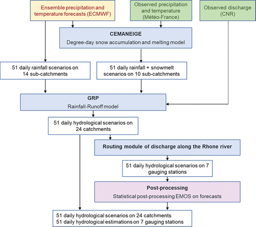
For 10 of the 24 catchments, located in mountainous areas, a snowmelt and accumulation model, CEMANEIGE (Valéry, 2010), feeds GRP. As catchments are not the same as the ones used in PHARE, GRP models are calibrated over 2012–2020 to reproduce observed daily discharge on each of the 24 considered sub-catchments. As for PHARE and the probabilistic short-term chain, the model is run during 1 year before the forecast, using observed precipitation and observed discharge data in an assimilation scheme to initialise GRP reservoirs before the forecast. A simple routine module allows us to propagate the forecasts from the tributaries towards seven gauging stations on the Rhône River.

An EMOS approach, calibrated on the 2008–2020 period, is then used on each time step to post-process forecasted streamflow on these gauging stations (Vannier et al., 2018). A validation of the EMOS approach is proposed in Section 5.2, showing the benefits of the method, in terms of bias and reliability. In contrast to the short-term forecasts, no ECC approach is used. Therefore, after this stage, seven univariate daily hydrological estimations are provided. Spatial coherence is not needed as this tool is a support for expertise and hydrological estimations and does not feed another tool. These estimations are available on seven gauging stations, whereas hydrological scenarios are available on 24 catchments corresponding to the main tributaries (see the left side of Figure 9).

An example forecast is given on the right side of Figure 9, under the “Raw” experiment for the hydrological forecasts derived from GRP and under the “Raw + EMOS” experiment for the hydrological forecast post-processed with EMOS.

4.3. Long-term (seasonal)

To optimise the commercialisation of its production, CNR needs to anticipate production trends for the 3 coming months. To do so, CNR performs monthly probabilistic production forecasts based on a statistical relationship using hydrometeorological data as input and calibrated with past data. For this tool, the Rhône River basin is divided into two zones: the Upper Rhône River and the Lower Rhône River (above and below the city of Lyon).

4.3.1. Data

CNR uses various types of data to perform its monthly production forecasts:

1. Potential production data aggregated at a monthly time step. Potential production is the production that CNR would have produced on the Rhône River considering operating constraints (such as current environmental flows) and no unavailability of production groups;

2. Information on operating constraints and the availability of production groups in the coming months;

3. Hydrometeorological data. CNR uses Météo-France CROCUS snow water equivalent (Vionnet et al., 2012), monthly Météo-France observed precipitation aggregated at catchment’s scale and observed flows from CNR stations on the Rhône River;

4. Seasonal forecasts from meteorological centres, for example from Météo-France.

4.3.2. Methods

The production forecast is based on a statistical model linking the temporal variation of potential production (the predictand) and hydrometeorological variables (the predictors), such as precipitation on the Rhône River main catchments, snow water equivalent on the Rhône River main tributaries and flows at CNR stations.

The relation is calibrated for each month of the forecast. For example, the calibration will link production during spring months to snow water equivalents in the Alps, or production during autumn and winter months to precipitation on specific catchments. Once calibrated, the forecaster applies the relation with the latest available data (flow, catchment precipitation and potential production of the previous month). The calibrated statistical relationship also needs information that is not known when the forecast is performed, such as rainfall for the coming months. To provide this, the forecaster defines qualitative meteorological trends (temperature, precipitations) on the Rhône River catchment for the 3 coming months, using available seasonal forecasts. For each month, the observed rainfall and temperature data of the previous years are used as input data to the statistical relationship, except for the years less consistent with the expected trends, which are discarded.

The uncertainty of this production forecast is based on the meteorological uncertainty for the coming months and on the goodness of fit of the statistical relationship. They are mixed to provide an ensemble forecast made of 100 potential productions for each month. This ensemble potential production forecast is then transformed into production using current and forecasted group unavailabilities and operating constraints, which are expressed as a percentage of the potential production.

The forecaster runs the model with different predictors. These runs, based on a multi-parameterisation of the model, are called scenarios. These scenarios allow us to study the sensitivity of the forecast quantiles to the input data. Finally, the forecaster analyses the various scenarios to issue the reference forecast. For this purpose, the forecaster weights each scenario according to the predictors used and the quality of the model in the calibration period. The reference forecast is calculated as the weighted average of the different scenarios and is later used by the team in charge of valuing production on the electricity market.

Figure 8 presents an example result, with three scenarios of production on the entire Rhône River basin made in December 2017 for January 2018, after the forecasters’ evaluation. Values of production on the y-axis have been voluntarily erased. Figure 8 shows that the forecasters predicted a wet trend, with a correct reliability. On the three scenarios, the 50^th and 95^th forecasted quantiles are above the historical ones, meaning that production in January 2018 is forecasted to be higher than a mean production computed on a reference period, by more than 50% of the ensemble members. The forecasted 5^th quantile is lower than the historical one, meaning that at least 5% of the forecasts predict a lower production than the historical one.

Figure 8. Forecasting scenarios of monthly production for January 2018 realised in December 2017.

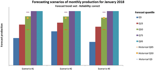
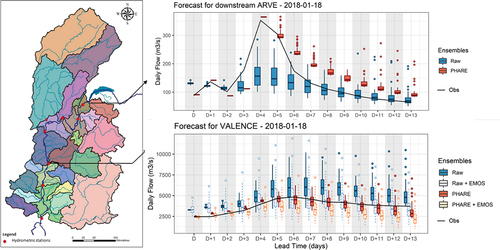
Figure 9. Probabilistic daily forecasts obtained for 18 January 2018, for two stations, with (PHARE, in red) and without (Raw, in blue) the integration of PHARE. The firstday of the forecast is named “D”. The EMOS post-processing appears in light blue for the Raw experiment, and orange for the PHARE experiment.

5. Human expertise and coherence between the tools

Human expertise is at the heart of CNR forecasts, and the above tools provide first estimates of hydrometeorological situations for different lead times on the Rhône River basin that can potentially be adjusted by forecasters. These adjustments are fully integrated into the deterministic chain (see Section 3 on OPALE and PHARE) and their integration is under development for the probabilistic tools. The mid- and long-term tools (Sections 4.2 and 4.3, respectively) allow simple human expertise, and further developments will be undertaken to integrate full human expertise into the short-term probabilistic forecasts (Section 4.1). These different tools are complementary, but they need to propagate the expertise in a coherent manner to provide an ensemble of hydrometeorological scenarios for different lead times. This section aims to provide an overview of the first attempts made to add some coherence between the hydrometeorological forecasting chains.

5.1. The role of forecasters in hydrometeorological tools

In the deterministic framework (see Section 3), forecasters analyse meteorological forecasts from various mesoscale models such as GFS, CEP and ICON Icosahedral Nonhydrostatic (see Table 1) to identify the preferred synoptic path over the forecast horizon. From this analysis, they use their expertise to build the most appropriate and probable precipitation scenario from the OPALE interface, considering the known biases of the different NWP models. With this same tool, the forecasters adjust the forecast of the rain–snow limit, defining a more accurate partitioning between liquid and solid precipitation. They also check snow data from the French weather forecast services as well as webcams available at some ski resorts. Then, forecasters estimate the merged inputs to each basin. At this stage, the forecasters have built the total incoming water (rainfall + snowmelt) for each catchment. This expert scenario is then used as input data for the hydrological step (the PHARE tool). In the case of meteorologically uncertain situations or flood events, a second expert precipitation scenario can be drawn. This alternative scenario is often used to consider a less probable weather evolution.

Regarding the hydrological step, forecasters create an expert hydrological scenario for each basin, considering the results of different hydrological models as a first guess. The expertise brought by the forecasters in this hydrological step includes knowledge of the hypotheses of the different models. To give an example based on Figure 4, according to personal experience, the forecaster knows that the GRP model tends to overestimate flows for similar hydrometeorological situations. The peak simulated by this model is above a 5-year return period flood, which represents a very high flow for mid-January. The forecaster chose to follow the dynamics of the GRP-model but also to slightly moderate the flow on short lead times and to limit the peak.

Finally, the forecasters define an optimised production program on the hydraulic tools, while ensuring hydraulic safety. They can thus define a reservoir management program for each hydropower development, that makes the best use of CNR limited intra-day storage. The forecasters can indeed define a program with increased production (and reservoir emptying) when electricity prices are high and decreased production (and reservoir filling) when electricity prices are low.

The need for longer lead times led CNR to develop a mid-term tool that includes an outlook of meteorological uncertainties with probabilistic forecasts (see Section 4.2). Here again, it is possible to include human expertise by manually shifting the median value of the 51 scenarios on the 24 catchments, for each of the 14 forecasted days. The initial spread around the median is kept and applied around the new median to provide a shifted box plot composed by the 51 values. The propagation module and the EMOS correction are then applied using the expertise on the catchments.

These two complementary tools are run in parallel by CNR forecasters who add manual expertise into the forecasts. In practice, information from both tools is useful to facilitate the inclusion of expertise into the other tool, and forecasters often must switch between the tools to make the information coherent. This is further complicated by the need to provide concise, practical, and coherent information to the final users for all the lead times (Day + 4 and Day + 14). This problem has led to the development of techniques to unify the two mentioned tools.

The forecasters also add their expertise into the long-term (seasonal) forecasts. They run the long-term model with different predictors and then weight the resulting estimations, based on the chosen predictors and the quality of the model (see Section 4.3.2).

5.2. Seamless combination of forecasts

First attempts to connect the deterministic short-term tool, PHARE (Section 3.3.2), and the probabilistic mid-term tool (Section 4.2) have been made. To do so, the outputs of PHARE (providing an hourly forecast with human expertise up to 4 days ahead) have been used in the mid-term probabilistic tool (providing daily probabilistic forecasts or estimations for the next 14 days). PHARE outputs available at the same stations as the ones used in the probabilistic tool are aggregated at a daily time step on their 4 days of availability. They are then used as observations in the data assimilation scheme of the probabilistic tool. To recall, the data assimilation scheme consists in defining the routing reservoir level in GRP, in order to match simulated to observed streamflow. Consequently, the probabilistic meteorological forecasts are only used from the 5^th day in the future.

Figure 9 provides an example of this combination for the forecast taking place on 18 January 2018. Two experiments are available for the downstream Arve River basin: the Raw experiment, which is the GRP output; and the PHARE experiment, which is the result of the above combination, using PHARE on the first 4 days as observations in the forecast. The GRP model is then run from the 5^th day. The added value of the integration of PHARE is clear as the flow peak is correctly estimated with the PHARE experiment, and not with the Raw experiment. Figure 9 also provides an example for the Valence Rhône River gauging station (bottom line). Two more experiments are available for this station, with the post-processing of the Raw and PHARE experiments with the EMOS method. Here again, the added value of the PHARE experiment is quite clear on this date. The EMOS method increases reliability, particularly on the first 4 days of the forecast where the PHARE experiment provides an ensemble with a small dispersion.

To assess the overall performance of the different experiments, the continuous ranked probability score (CRPS; Hersbach, 2000) is computed for each lead time, for the forecasts in the 2008–2020 period. This score is equivalent to a quadratic measure of the difference between the forecast cumulative density function and the observed cumulative density function. Figure 10 provides the continuous ranked probability skill score (CRPSS), computed following Equation (3)(3) $CRPSS=1-\hspace{0.17em}\frac{CRPS}{CRP{S}_{ref}}$(3) :

Figure 10. CRPSS obtained for the three different experiments, using the Raw experiment as a reference, on the seven gauging stations on the Rhône River.

(3) $CRPSS=1-\hspace{0.17em}\frac{CRPS}{CRP{S}_{ref}}$(3)

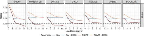
The CRPSS has an optimal value of 1. A value between 0 and 1 means that the evaluated experiment performs better than the one used as reference, whereas a value of less than 0 means that the evaluated experiment performs worse than the one used as reference. The reference experiment used is the Raw experiment. Three scores are then obtained for each lead time, with the Raw + EMOS, PHARE, and PHARE + EMOS experiments. Figure 10 shows that the PHARE + EMOS experiment has the best score, with a CRPSS of around 0.5 for the first forecasted days, slowly decreasing to around 0.25 for the last lead times, joining the CRPSS from the Raw + EMOS experiment. The added value of the integration of PHARE is quite visible for the first lead times but drops between the 5^th and 6^th days if the EMOS post-processing is not used. This is due to the reliability term composing the CRPS, the experiments with PHARE having less reliability than the Raw experiment, especially for the Upper Rhône River stations (before Ternay).

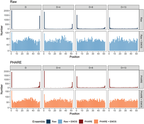
Figure 11 confirms the importance of the EMOS post-processing method, showing a ranking diagram for four different lead times for the Valence station and the four experiments. This rank histogram counts the number of days the observation is at a position between 1 and 52 in the ensemble, for each lead time (the period of reference is 2008–2020). A position of 1 means that the ensemble overestimates the observation, whereas a position of 52 means that the ensemble underestimates the observation. A reliable forecast is obtained when the rank histogram is flat, meaning an equivalent distribution of the observation inside the ensemble. The Raw experiment is under-dispersive at the first lead time and biased at the other lead times, whereas the PHARE experiment is constantly biased. The EMOS post-processing approach allows us to retrieve a quite flat histogram, and to largely improve reliability, for both the Raw and PHARE experiments.

Figure 11. Rank histogram for the four experiments at the first lead time (day D) and 4, 8 and 13 days after (D + 4, D + 8, D + 13) for the Valence station.

Improving the coherence between these tools – and thus, their forecasts – results in a better understanding of the long-term processes for the forecasters, and in technical support for the expertise. As evaluated in Figures 9, 10 and 11, the added value of the PHARE + EMOS forecasts is significant. This combination integrates the expertise into the probabilistic mid-term tool. This development is also considered to combine the mid-term probabilistic tool (Section 4.2) with the sub-seasonal probabilistic tool (Section 4.3).

5.3. Ongoing developments

Ongoing developments aim to improve the seamless combination presented in Section 5.2 by keeping the uncertainty provided by probabilistic forecasts on the first lead times while assimilating the deterministic forecasts from PHARE. The technique presented in Section 5.2 will then be used to link all the tools (short-term, mid-term and long-term) to create a unique forecasting outlook for the Rhône River.

An important task remains to find a way to combine the human expertise of forecasters with short-term probabilistic forecasts, without losing the valuable information they provide on uncertainties. This implies the necessity to rethink the way expertise on scenarios should be used, as well as the scale (both temporal and spatial) at which to perform it.

Furthermore, a complete redesign of the PHARE tool is being undertaken to visually integrate the results of the probabilistic tools. This step will provide figures displaying deterministic forecasts as lines, but also probabilistic forecasts in various forms (box plots, lines, statistics), overlying the deterministic results. This will allow forecasters to assess the coherence between deterministic and probabilistic forecasts and to add expertise considering the results of all the different tools.

6. Conclusion and perspectives

This article introduces the different tools used at CNR to provide hydrometeorological forecasts at different lead times on the tributaries of the Rhône River. Four complementary tools are currently used by CNR forecasters to manage the river and to optimise hydropower production for the energy wholesale market. Deterministic hourly hydrometeorological forecasts are available for the next 4 days with the OPALE and PHARE tools. A probabilistic version of these tools is currently being developed to consider hydrometeorological uncertainties. A daily probabilistic tool provides hydrometeorological data up to the next 14 days, here again for optimisation production purposes and due to the need to schedule maintenance on hydroelectric facilities. Finally, a seasonal probabilistic tool provides seasonal estimates of production for the next 3 months. All these tools are adapted to the forecasting context in terms of computational time. The short-term deterministic chain takes approximately 5 minutes to run, the short-term probabilistic chain takes approximately 15 to 20 minutes, and the mid-term probabilistic chain takes approximately 5 minutes.

These tools are combined with human expertise, which plays an important role in the design of the forecasts. The expertise of the forecasters is fully integrated in the short-term deterministic tool, and studies are in progress to allow its integration into the probabilistic tools. The development of all these tools has further increased the need for coherence between the different forecasts, and first attempts have been made to combine information between the short-term and mid-term hydrological forecasts.

Other developments will also focus on the downstream part of the forecasting chain, i.e. on the use of probabilistic hydrological forecasts in the decision-making process. CNR is committed to an ambitious project to develop a new version of an automated optimisation tool (POMMIER) dedicated to facilitating the joint optimisation of the Rhône assets with the CNR intermittent wind and solar power generation. This tool will consider uncertainties using ensemble coherent production forecasts from the three types of energy, and market price scenarios. Such a tool will use as input the results of the probabilistic forecasting chain described here for hydropower production.

Disclosure statement

No potential conflict of interest was reported by the authors.

References

- Addor, N., Jaun, S., Fundel, F., & Zappa, M. (2011). An operational hydrological ensemble prediction system for the city of Zurich (Switzerland): Skill, case studies and scenarios. Hydrology and Earth System Sciences, 15(7), 1–18. https://doi.org/10.5194/hess-15-2327-2011
- Bellier, J. (2018). Prévisions hydrologiques probabilistes dans un cadre multivarié : Quels outils pour assurer fiabilité et cohérence spatio-temporelle ? [PhD thesis in Ocean, Atmosphère].
- Bellier, J., Bontron, G., & Zin, I. (2017). Using meteorological analogues for reordering postprocessed precipitation ensembles in hydrological forecasting. Water Resources Research, 53(12), 10085–10107. https://doi.org/10.1002/2017WR021245
- Bellier, J., Zin, I., & Bontron, G. (2018). Generating coherent ensemble forecasts after hydrological postprocessing: adaptations of ECC‐based methods. Water Resources Research, 54(8), 5741–5762. https://doi.org/10.1029/2018WR022601
- Bellier, J., Bontron, G., & Zin, I. (2021). Selecting components in a probabilistic hydrological forecasting chain: The benefits of an integrated evaluation. LHB: Hydroscience Journal, 107(1), 1938352. https://doi.org/10.1080/27678490.2021.1936825
- Ben Daoud, A., Sauquet, E., Bontron, G., Obled, C., & Lang, M. (2016). Daily quantitative precipitation forecasts based on the analogue method: Improvements and application to a French large river basin. Atmospheric Research, 169(A), 147–159. https://doi.org/10.1016/j.atmosres.2015.09.015
- Bennett, J. C., Wang, Q. J., Robertson, D. E., Schepen, A., Li, M., & Michael, K. (2017). Assessment of an ensemble seasonal streamflow forecasting system for Australia. Hydrology and Earth System Sciences, 21(12), 6007–6030. https://doi.org/10.5194/hess-21-6007-2017
- Berthet, L. (2010). Prévision des crues au pas de temps horaire : pour une meilleure assimilation de l’information de débit dans un modèle hydrologique [PhD thesis in Hydrology]. Institut des Sciences et Industries du Vivant et de l’Environnement, AgroParisTech.
- Berthet, L., Andréassian, V., Perrin, C., & Javelle, P. (2009). How crucial is it to account for the antecedent moisture conditions in flood forecasting? Comparison of event-based and continuous approaches on 178 catchments. Hydrology and Earth System Sciences, 13(6), 819–831. https://doi.org/10.5194/hess-13-819-2009
- Berthet, L., Valéry, A., Garçon, R., Marty, R., Moulin, L., Puygrenier, D., Piotte, O., Le Lay, M., Janet, B., & Duquesne, F. (2019). Cohérence des prévisions et place de l’expertise : Les nouveaux défis pour la prévision des crues. La Houille Blanche, 1, 5–12.
- Bompart, P., Bontron, G., Celié, S., & Haond, M. (2008). An operational hydrometeorological forecasting chain for CNR’s hydroelectric production needs. La Houille Blanche, 5, 54–60.
- Bontron, G. (2004). Prévision quantitative des précipitations: Adaptation probabiliste par recherche d’analogues. Utilisation des réanalyses NCEP-NCAR et application aux précipitations du Sud-Est de la France [PhD thesis]. Institut National Polytechnique de Grenoble.
- Bougeault P., Toth, Z., Bishop, C., Brown, B., Burridge, D., Chen, D. H., Ebert, B., Fuentes, B., Hamill, T. M., Mylne, K., Nicolau, J., Paccagnella, T., Park, Y.-Y., Parsons, D., Raoult, B., Schuster, D., Silva Dias, P., Swinbank, R., Takeuchi, Y., Tennant, W., Wilson, L., & Worley, S. (2010). The THORPEX interactive grand global ensemble. Bulletin of the American ,Meteorological Society, 91(8), 1059–1072. https://doi.org/10.1175/2010bams2853.1
- Carriere, T., Vernay, C., Pitaval, S., & Kariniotakis, G. (2020, May). A novel approach for seamless probabilistic photovoltaic power forecasting covering multiple time frames. IEEE Transactions on Smart Grid, 11(3), 2281–2292. https://doi.org/10.1109/TSG.2019.2951288
- Celié, S., Bontron, G., Ouf, D., & Pont, E. (2019). Apport de l’expertise dans la prévision hydrométéorologique opérationnelle. La Houille Blanche, 105(2), 55–62. https://doi.org/10.1051/lhb/2019015
- Cloke, H. L., & Pappenberger, F. (2009). Ensemble flood forecasting: A review. Journal of Hydrology, 375(3–4), 613–626. https://doi.org/10.1016/j.jhydrol.2009.06.005
- Demargne, J., Wu, L., Regonda, S. K., Brown, J. D., Lee, H., He, M., Seo, D., Hartman, R., Herr, H. D., Fresch, M., Schaake, J., & Zhu, Y. (2014). The science of NOAA’s operational hydrologic ensemble forecast service. Bulletin of the American Meteorological Society, 95(1), 79–98. https://doi.org/10.1175/BAMS-D-12-00081.1
- Demeritt, D., Nobert, S., Cloke, H. L., & Pappenberger, F. (2010). Challenges in communicating and using ensembles in operational flood forecasting. Meteorological Applications, 17(2), 209–222. https://doi.org/10.1002/met.194
- Desaint, B., Nogues, P., Perret, C., & Garçon, R. (2009). La prévision hydrométéorologique opérationnelle: L’expérience d’Electricité de France. La Houille Blanche, 95(5), 39–46. https://doi.org/10.1051/lhb/2009054
- Gneiting, T., Raftery, A. E., Westveld, A. H., & Goldman, T. (2005). Calibrated probabilistic forecasting using ensemble model output statistics and minimum CRPS estimation. Monthly Weather Review, 133(5), 1098–1118. https://doi.org/10.1175/MWR2904.1
- Grimaldi, L., Bontron, G., Balayn, P. (2014). Hydraulic modelling for Rhône River operation. In P. Gourbesville, J. Cunge, & G. Caignaert (Eds.), Advances in hydroinformatics (pp. 35–45). Springer Hydrogeology. https://doi.org/10.1007/978-981-4451-42-0_4
- Hersbach, H. (2000). Decomposition of the continuous ranked probability score for ensemble prediction systems. Weather and Forecasting, 15(5), 559–570. https://doi.org/10.1175/1520-0434(2000)015<0559:DOTCRP>2.0.CO;2
- Lorenz, E., Kühnert, J., Heinemann, D. (2014). Overview of irradiance and photovoltaic power prediction. In A. Troccoli, L. Dubus, & S. Haupt (Eds.), Weather matters for energy (pp. 429–454). Springer. https://doi.org/10.1007/978-1-4614-9221-4_21
- Molteni, F., Buizza, R., Palmer, T. N., & Petroliagis, T. (1996). The ECMWF ensemble prediction system: Methodology and validation. Quarterly Journal of the Royal Meteorological Society, 122(529), 73–119. https://doi.org/10.1002/qj.49712252905
- Moulin, L., Abonnel, A., Puygrenier, D., Valéry, A., & Garçon, R. (2019). Prévision hydrométéorologique opérationnelle à EDF-DTG – Progrès récents et état des lieux en 2018. La Houille Blanche, 105(2), 44–54. https://doi.org/10.1051/lhb/2019014
- Obled, C., Bontron, G., & Garçon, R. (2002). Quantitative precipitation Forecasts: A statistical adaptation of model outputs through an analog sorting approach. Atmospheric Research, 63(3/4), 303–324. https://doi.org/10.1016/S0169-8095(02)00038-8
- Pagano, T. C., Wood, A. W., Ramos, M., Cloke, H. L., Pappenberger, F., Clark, M. P., Cranston, M., Kavetski, D., Mathevet, T., Sorooshian, S., & Verkade, J. S. (2014). Challenges of operational river forecasting. Journal of Hydrometeorology, 15(4), 1692–1707. https://doi.org/10.1175/JHM-D-13-0188.1
- Piron, V., Bontron, G., & Pochat, M. (2015). Operating a hydropower cascade to optimize energy management. Hydropower & Dams, 22(5). https://www.hydropower-dams.com/articles/operating-a-hydropower-cascade-to-optimize-energy-management/
- Raftery, A. E., Gneiting, A., Balabdaoui, F., & Polakowski, M. (2005). Using Bayesian model averaging to calibrate forecast ensemble. Monthly Weather Review, 133(5), 1155–1174. https://doi.org/10.1175/MWR2906.1
- Ramos, M. H., Van Andel, S. J., & Pappenberger, F. (2013). Do probabilistic forecasts lead to better decisions? Hydrology and Earth System Sciences, 17(6), 2219–2232. https://doi.org/10.5194/hess-17-2219-2013
- Remesan, R., & Mathew, J. (2015). Hydrological data driven modelling. A case study approach. Springer.
- Schefzik, R., Thorarinsdottir, T., & Gneiting, T. (2013). Uncertainty quantification in complex simulation models using ensemble copula coupling. Statistical Science, 28(4), 616–640. https://doi.org/10.1214/13-STS443
- Thielen, J., Bartholmes, J., Ramos, M.-H., & De Roo, A. (2009a). The European flood alert system part 1: Concept and development. Hydrology and Earth System Sciences, 13(2), 125–140. https://doi.org/10.5194/hess-13-125-2009
- Thielen, J., Bogner, K., Pappenberger, F., Kalas, M., Del Medicoa, M., & de Rooa, A. (2009b). Monthly-, medium-, and short-range flood warning: Testing the limits of predictability. Meteorological Applications, 16 (1), 77–90. (2009). https://doi.org/10.1002/met.140
- Troin, M., Arsenault, R., Wood, A. W., Brissette, F., & Martel, J.-L. (2021). Generating ensemble streamflow forecasts: A review of methods and approaches over the past 40 years. Water Resources Research, 57(7), e2020WR028392. https://doi.org/10.1029/2020WR028392
- Valéry, A. (2010). Modélisation précipitations – Débit sous influence nivale. Élaboration d’un module neige et évaluation sur 380 bassins versants [PhD Thesis]. AgroParisTech.
- Vannier, O., Celie, S., Legrand, S., & Bellier, J. (2018). A first use case of operationnal ensemble discharge forecasts for hydropower production on the Rhône River: Evaluation on several post-processing methods. 2018 HEPEX Workshop.
- Vionnet, V., Brun, E., Morin, S., Boone, A., Faroux, S., Le Moigne, P., Martin, E., & Willemet, J.-M. (2012). The detailed snowpack scheme Crocus and its implementation in SURFEX v7.2. Geoscientific Model Development, 5(3), 773–791. https://doi.org/10.5194/gmd-5-773-2012
- Wetterhall, F., & Di Giuseppe, F. (2018). The benefit of seamless forecasts for hydrological predictions over Europe. Hydrology and Earth System Sciences, 22(6), 3409–3420. https://doi.org/10.5194/hess-22-3409-2018
- Zalachori, I., Ramos, M. H., Garçon, R., Mathevet, T., & Gailhard, J. (2012). Statistical processing of forecasts for hydrological ensemble prediction: A comparative study of different bias correction strategies. Advances in Science and Research, 8(1), 135–141. https://doi.org/10.5194/asr-8-135-2012