Evaluation of Value-at-Risk (VaR) using the Gaussian Mixture Models

Abstract

The normality of the distribution of stock returns is one of the basic assumptions in financial mathematics. Empirical studies, however, undermine the validity of this assumption. In order to flexibly fit complex non-normal distributions, this article applies a Gaussian Mixture Model (GMM) in the context of Value-at-Risk (VaR) estimation. The study compares the forecasting ability of GMM with other widespread VaR approaches, scrutinizing the data on the daily log-returns for a wide range of “S&P 500” stocks in two periods: from 2006 to 2010 and from 2016 to 2021. The statistical and graphical analysis revealed that GMM quickly and adequately adjusts to significant and rapid stock market changes, although the remaining methods delay. The study also found that the ratio of short-term and long-term standard deviations significantly improves the GMM and other methods’ ability to predict VaR, reflecting the observed features of analyzed stock log-returns.

Keywords:

• Gaussian Mixture Model
• normal distribution
• heavy tails
• Value-at-Risk
• Monte-Carlo simulations
• backtesting

1. Introduction

Many applied financial mathematics models rely on efficient market hypothesis and perceive stock returns as independent and normally distributed. Yet Mandelbrot (1963) revealed that financial data is more likely to follow asymmetric, heavy-tailed distributions that admit large deviations. Frequent and severe socioeconomic changes further undermine the reliability of the normality assumption. In 2020, the announcement of the coronavirus pandemic led to rapid market behavior changes when staying-at-home consumers significantly reduced their spending on non-basic goods and services. These excess savings allowed US households, just in 6 months (November 2020–April 2021), to invest more money in stock funds than in the earlier 12 years, respectively, 569 and 452 bln. USD (Cox 2021). In 2022, the annual US inflation hiked at 7.5%—the heights not seen in 40 years (Cox 2022). Besides, Russia’s invasion of Ukraine in February 2022, nuclear war threats, and the energy crisis boosted uncertainty of future economic growth, adding to further reduction of the “S&P 500”, “Nasdaq 100”, and other US stock prices (Dey 2022). The nature of the most recent events, hence, differs from that of the global financial crisis of 2007–2008, which was purely rooted in the distortions related to financial markets. In a financial crisis, asset prices see a steep decline in value, businesses and consumers are unable to pay their debts, and financial institutions experience liquidity shortages. A financial crisis is often associated with a panic or a bank run, during which investors sell off assets or withdraw money from savings accounts because they fear that the value of those assets will drop if they remain in a financial institution.

In responding to the above shocks, effective risk management becomes an integral part of investments that aim to mitigate possible losses and earn higher returns. For nearly 30 years, one of the most widespread risk assessment methods is the Value-at-Risk (VaR) model. VaR estimates the value that the loss will not exceed with X percent probability in the next N days (Hull 2015). However, since 2012, the Basel Committee has initiated discussions on the need to change the VaR model to Expected Shortfall (ES) (Hull 2015). Such a change should appear in the new publication of regulations “Basel IV” for which the implementation date is postponed to January 2025. VaR is the basis of the ES model, as the latter calculates the conditional expectation of losses exceeding the VaR value. In the future, after the ES model is implemented in businesses and more technical standards are defined, it can serve as a standalone research topic.

Variance-Covariance (VC), Historical Modeling (HM), and Monte-Carlo (MC) simulation methods are among the most widespread VaR calculation approaches. In 1996, “JP Morgan” published VaR technical documentation introducing the VC approach (Morgan 1996). Although the VaR model was already known and applied by then, the “JP Morgan” paper drastically popularized its application. The VC method assumes the normal distribution of the profit-loss (PL) measure. Meanwhile, the HM approach asserts that the historical PL distribution remains the same as in the historical period, and there is no need to define an exact theoretical distribution (Hull 2015). The MC simulation method is similar to the historical one but, instead of taking historical data distribution, generates the changes in risk factors using, for example, a geometric Brownian motion (GBM) process in which a Gaussian distribution appears.

Developing more realistic VaR methods that, contrary to VC and MC GBM methods, do not rely on the often invalid normality assumption, as a reasonable option, researchers propose the Gaussian Mixture Model (GMM). Tan (2005), Tan and Tokinaga (2007), Tan and Chu (2012) showed that the GMM distribution can adequately account for key stylized facts such as heavy tails and asymmetry, being relatively simple compared to distributions such as Student or Generalized Normal.

Furthermore, Contreras (2014) assessed the VaR model, comparing such methods as parametric Delta, HM, and Delta-GMM. Bypassing exact derivation, Contreras showed that the VaR metric for Delta-GMM follows from solving $F_L(q_{\alpha };\mathit{\omega },\mathit{\mu },\mathit{\sigma })-\alpha =0$ with respect to q_α, where F_L is the loss distribution function; $\mathit{\omega },\mathit{\mu },\mathit{\sigma }$ are GMM parameters (see Section 3); q_α is an α-quantile. The empirical results revealed that GMM and HM likewise predict VaR values for the portfolio, which consists of stocks, bonds, and currency derivatives. However, GMM adapts to varying risk factors much faster by changing 𝝎 parameters (see Section 3). The VaR method based on the assumption of normality performed the worst, which significantly underestimated values. Similar conclusions are in Cuevas-Covarrubias et al. (2017) paper, where the authors propose to reconsider the appropriateness of the normal distribution in risk management and quantitative finance theory, paying more attention to the GMM.

Sarkar et al. (2018) and Wang et al. (2020) allocate the GMM to unsupervised machine learning approaches when the parameters of the model are estimated using K-means and Expectation-Maximization (EM) algorithms. Despite the widespread view that the behavior of financial markets resembles a black box with hardly predictable outputs, GMM can discover and independently learn relationships and structures in large data arrays, based on which researchers get meaningful insights about the analyzed data.

Our research elaborates on the Seyfi et al. (2021) paper that describes how to predict VaR values using GMM together with clustering algorithms. The authors also conclude that the GMM method can better account for the risks in the tails and adapt more quickly to volatile market conditions. In addition, the authors proposed to adjust the stock returns obtained with GMM by multiplying them by the ratio σ_[70]∕σ_[250], where σ_[x] is the standard deviation of the last x days, arguing that this will allow the model to adapt even faster to changing market conditions. VaR models are often used in conjunction with Exponential Weighted Moving Averages (EWMAs) by assigning exponentially declining weights to older observations (Morgan 1996). Such a multiplier is based on a tuning parameter λ which can be chosen based on cross-validation. In contrast, the distinctive aspect of σ_[70]∕σ_[250] is that it is estimated directly from stock return data. Besides, this volatility multiplier similarly improves VaR prediction accuracy with a shorter calibration period for VaR models, although simultaneously satisfying regulatory requirements that the model be calibrated for at least one year (approx. 250 days) based on historical observations. To ensure a fair comparison across methods, our paper incorporates the volatility multiplier into all examined VaR approaches, encompassing traditional methods. Moreover, we evaluate the benefits and drawbacks of this supplementary multiplier for one-day VaR predictions through visual representation and statistical backtesting analysis.

This article aims to show that the GMM is a practical financial modeling tool and can be significantly superior to other widespread VaR methods in predicting losses even in periods of increased volatility: the 2007–2008 global financial crisis and the market shock caused by COVID-19. Furthermore, additional statistical analysis revealed that the GMM distribution closely tracks the observed unimodal and heavy-tailed distribution (see Definition 3.1 and considerations below) of the analyzed stock log-returns. Accordingly, a sufficient condition for the unimodal probability density of GM distribution with two components is given, along with the necessary extended proofs. In addition, the conditions are formulated to define when the tails of the GM distribution can be heavier than the tails of a single normal distribution. Moreover, it has been noticed that the GMM can be used as an additional tool in market risk reporting, including VaR model breach analysis. Information about GMM components and their weights helps determine whether the market is currently experiencing increased or decreased volatility and whether positive or negative returns prevail. Also, a detailed backtesting of different VaR methods and a comparative analysis of predictions nominated the GMM method as the most appropriate, closely followed by the HM approach, while the normality assumption-based VC and MC methods were the least fit for the analyzed data.

The article is structured as follows. Section 2 analyses the features of the data taken in the periods that include the financial crisis (2006–2010) and COVID-19 pandemic (2016–2021) events. Section 3 discusses the theoretical underpinnings and practical aspects of the GMM approach applied in the VaR context. Section 4 provides a backtesting methodology, while Section 5 scrutinizes one-day VaR model predictions comparing with the outcomes of two analyzed periods. Section 6 concludes.

2. Data analysis

According to Taleb (2008), the metaphor “black swan” refers to shocking and unforeseen events (e.g., war, financial crisis, pandemic, energy supply shortage). In financial markets, such events can cause extremely significant losses. Adams and Thornton (2013) conclude that VaR models are useful in predicting losses with a high confidence level, but they are incapable of predicting extreme or catastrophic losses based on historical data.

Seeking a more accurate identification of the differences between the VaR methods, we conducted a comparative analysis of the stock market data for two extremely volatile periods. The first period is from 01/03/2006 to 12/31/2010 (a total of 1,260 trading days), which includes the global financial crisis of 2007–2008. The second is the market turbulence period caused by the COVID-19 pandemic—from 01/04/2016 to 12/31/2021 (a total of 1,511 trading days). In addition to stressful periods, the selected time ranges also include more stable intervals, allowing comparisons of the models’ performances to be made between calm and volatile intervals, as the model should be able to work adequately in different volatility periods. Even for very stable time intervals, the model may not be the most appropriate due to the possibility of becoming too conservative, resulting in higher capital requirements and inefficient use of capital.

In this study, an equally weighted portfolio of almost all “S&P 500” index stocks¹ is used. In total, 416 stocks are analyzed, while other stocks are eliminated to have identical and comparable portfolios across both time periods. Box plots below display the main characteristics of all stocks analyzed.

The descriptive statistics of 2006–2010 in Figure 1 show that approximately half of the stocks have positively skewed distributions, while the other half are negatively skewed. For positively skewed stocks, average of log-returns is larger than the median, which means that distributions have heavier right tails. Furthermore, the kurtosis coefficients are far from zero, indicating that density functions of stock return distributions decay faster and they have heavier tails than the normal distribution. In addition, the Jarque-Bera test³ rejects the hypothesis of normality of log-returns for all analyzed stocks.

Figure 1. Descriptive statistics of stock log-returns², 2006–2010.²The charts are improved by removing a few outlier values for skewness (less than -6) and kurtosis (greater than 100).

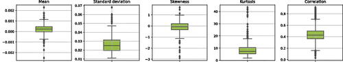
Heavier tails of the log-returns distribution indicate that investments are riskier. Also, the correlation among various stock pairs is positive, resulting in a lower diversification benefit, overreaction to systematic risk, and higher portfolio volatility. These conclusions follow from the Law of Diversification pioneered by Harry Markowitz (1952) in Modern Portfolio Theory. Assessing the diversification impact is straightforward: compare the sum of individual stock VaR measures to that of a portfolio. Higher-correlated stocks result in a smaller diversification effect. For instance, AmerisourceBergen (ABC) and Arthur J. Gallagher & Co. (AJG) have a correlation of 0.23, while Albemarle Corporation (ALB) and Weyerhaeuser (WY) show 0.61. A portfolio with less correlated stocks boasts 59% diversification, whereas a more correlated portfolio sees a 10% smaller effect.

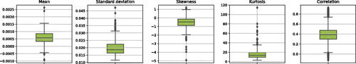
On the other hand, results for the 2016–2021 period in Figure 2 show that the majority of stocks have a negatively skewed distribution. This statistic has a median value below zero and numerous outlying negative values. Such skewness measures indicate that the mean is less than the median, i.e., the data likely has large negative outliers too. Also, in the COVID-19 pandemic period, kurtosis values were substantially higher than in 2006–2010, providing even greater confidence in rejecting normality hypotheses and bringing JB test p-values for all stocks close to zero. However, the distribution of standard deviations associated with the average log-returns uncertainty is relatively smaller than during the global financial crisis. Although the correlation among various stock pairs is mainly positive, there are also negative coefficients, which were not observed during the stressful period of 2006–2010.

Figure 2. Descriptive statistics of stock log-returns, 2016–2021.

3. Gaussian Mixture Model

Gaussian Mixture Model (GMM) is a probabilistic model based on the assumption that the data originates from a finite number of Gaussian distributions (Rudin 2021). In general, the data generation process with mixture models involves two steps:

1. Generate latent variables $z_i|\mathit{\omega }\sim \mathrm{Categorical}(\mathit{\omega })$, where $\mathit{\omega }=\{{\omega }_1,\dots ,{\omega }_{N_c}\}$ is a vector of mixture weights, ${\sum }_{j=1}^{N_c}{\omega }_j=1,0<{\omega }_j<1$;

2. Simulate $x_i|z_i=j\sim N({\mu }_j,{\mathrm{\Sigma }}_j)$ variables based on z_i values, where μ_j, Σ_j – the mean and covariance matrix of the j-th cluster, $j=1,\dots ,N_c$.

Thus, the density of the GMM is the weighted sum of $N(\mathit{\mu }\in {\mathbb{R}}^k,\mathbf{\Sigma }\in {\mathbb{R}}^{k\times k})$ probability density functions: $$\begin{array}{l}p(x_i)=\sum _{j=1}^{N_c}{\omega }_{j}f(x_i|{\mu }_j,{\mathrm{\Sigma }}_j).\end{array}$$

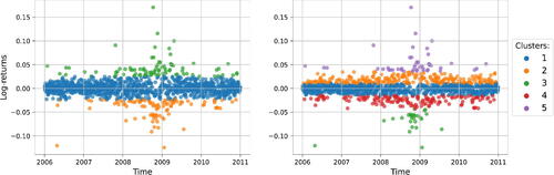
The main idea of the GMM is that each component (cluster) is a distinct normal distribution that describes different data sets. In the market risk context, such groups denote stock market states, e.g., the state of increased volatility or, conversely, decreased (see Figure 3, the color represents the state with the highest probability). Moreover, mixture weights $P(z_i=j|\mathit{\omega })={\omega }_j$ show how often market states change. For instance, suppose there is a recent escalation in market volatility paired with an abnormal increase in negative returns. Then, the GMM allocates higher weights to the normal distribution, whose parameters (mean and variance) accurately reflect this market condition. As a result, it is less likely to choose other normal distributions when simulating returns. This strategic weighting mechanism (regime-switching) assists the GMM model in adapting more swiftly to changing market conditions, ultimately resulting in more accurate log-return estimates.

Figure 3. Clustering “Microsoft” (MSFT) log-returns with GMM N_c = 3 and N_c = 5, 2006–2010.

3.1. Statistical properties

This subsection examines the unimodality and tail heaviness of the Gaussian Mixture (GM) distribution. For simplicity, the analysis uses the GM model with two components.

3.1.1. Unimodal density

The density curve of any unimodal distribution reaches its maximum value only at one point x = ν (mode), and values of function decrease when x recedes from ν. However, the distribution of stock log-returns can have more than one mode, but in this case, the unimodal distribution would not be appropriate. In the presence of other modes, the unimodal distribution would generate biased, inaccurate stock log-returns, and result in biased risk measures.

Analyzing the histograms of stock log-returns can help intuitively test if the data distribution is unimodal. Due to the wide range of “S&P 500” stocks, the unimodality of each distribution of stock log-returns is tested statistically with the Hartigan Dip (HD) test. This test determines whether the data distribution is similar to the unimodal distribution (Hartigan and Hartigan 1985). The outcomes of the HD test⁴ reveal that the hypothesis of unimodality is accepted for all stocks across two periods because p-values are greater than α = 0. 01. This short analysis shows that distributions of analyzed stock log-returns are unimodal. Therefore, an accurate assessment of the data-generating process requires determining the conditions when the GM distribution is unimodal.

Eisenberger (1964) derived sufficient conditions when GM distribution is unimodal or bimodal.

Lemma 3.1.

(Eisenberger 1964)Set that $Y_i\sim N({\mu }_i,{\sigma }_i^2),i=1,2$ are components of the Gaussian Mixture distribution. Density of Gaussian Mixture p(x, ω) is unimodal for all ω, $0<\omega <1$ when the following inequality is satisfied: $$\begin{array}{l}({\mu }_2-{\mu }_1{)}^2<{\displaystyle \frac{27{\sigma }_1^2{\sigma }_2^2}{4({\sigma }_1^2+{\sigma }_2^2)}}.\end{array}$$

The proof of Lemma 3.1 is provided in Appendix, including the additional theoretical justification of the inequality’s right-hand side omitted in the original proof.

3.1.2. Heavier tails

Heavier tails are a paramount feature of GM distribution that allows for evaluating stock log-returns more accurately, while normal distribution is incapable of such implementation.

Lemma 3.2.

(Feller 1968)Suppose that $X\sim N(0,1)$ and x > 0. Tails of the standard normal distribution $\mathrm{\Phi }(x)={\displaystyle \frac{1}{\sqrt{2\pi }}}{\int }_{-\mathrm{\infty }}^x{\mathrm{e}}^{-u^2/2}\mathrm{du}$ meets the following inequalities: (1) $$\begin{array}{l}{\displaystyle \frac{1}{\sqrt{2\pi }}}({\displaystyle \frac{1}{x}}-{\displaystyle \frac{1}{x^3}}){\mathrm{e}}^{-x^2/2}\le 1-\mathrm{\Phi }(x)=\overline{\mathrm{\Phi }}(x)\le {\displaystyle \frac{1}{x\sqrt{2\pi }}}{\mathrm{e}}^{-x^2/2}.\end{array}$$(1)

Assume that $Y\sim N(\mu ,{\sigma }^2)$. According to (1(1) $$\begin{array}{l}{\displaystyle \frac{1}{\sqrt{2\pi }}}({\displaystyle \frac{1}{x}}-{\displaystyle \frac{1}{x^3}}){\mathrm{e}}^{-x^2/2}\le 1-\mathrm{\Phi }(x)=\overline{\mathrm{\Phi }}(x)\le {\displaystyle \frac{1}{x\sqrt{2\pi }}}{\mathrm{e}}^{-x^2/2}.\end{array}$$(1) ) we get: $$\begin{array}{ll}P(Y>x)& =P({\displaystyle \frac{Y-\mu }{\sigma }}>{\displaystyle \frac{x-\mu }{\sigma }})=\overline{\mathrm{\Phi }}\left({\displaystyle \frac{x-\mu }{\sigma }}\right)\sim {\displaystyle \frac{\sigma }{\sqrt{2\pi }x}}{\mathrm{e}}^{-(x-\mu {)}^2/2{\sigma }^2}\\ & ={\displaystyle \frac{\sigma {\mathrm{e}}^{-{\mu }^2/(2{\sigma }^2)}}{\sqrt{2\pi }x}}{\mathrm{e}}^{-x^2/(2{\sigma }^2)}{\mathrm{e}}^{\mathrm{x\mu }/{\sigma }^2},x\to \mathrm{\infty }.\end{array}$$

Definition 3.1.

Suppose that $Y_i\sim N({\mu }_i,{\sigma }_i^2),i=1,2$ and $G(x):=\mathrm{\omega P}(Y_1\le x)+(1-\omega )P(Y_2\le x)$, $0<\omega <1$. Tails of distribution with distribution function G(x) are heavier than $Y\sim N(\mu ,{\sigma }^2)$ if the following property holds: $$\begin{array}{l}{\displaystyle \frac{\overline{G}(x)}{P(Y>x)}}={\displaystyle \frac{1-G(x)}{P(Y>x)}}\to \mathrm{\infty },\text{ as }x\to \mathrm{\infty }.\end{array}$$

This property shows that the probabilities of the GM distribution for higher values of stock log-returns tend slower to zero than that of a single Gaussian distribution; hence, the ratio of tail probabilities will tend to infinity. Otherwise, the tails of the GM distribution would be lighter than a normal distribution if the ratio tends to zero.

When ${\sigma }_1\ne {\sigma }_2\ne \sigma$ and x→∞: $$\begin{array}{ll}{\displaystyle \frac{\overline{G}(x)}{P(Y>x)}}& ={\displaystyle \frac{\omega {\sigma }_1}{\sigma }}\exp \left\{x^2({\displaystyle \frac{1}{2{\sigma }^2}}-{\displaystyle \frac{1}{2{\sigma }_1^2}})\right\}\exp \{{\displaystyle \frac{{\mu }_1^2}{{\sigma }_1^2}}-{\displaystyle \frac{{\mu }^2}{{\sigma }^2}}\}\exp \left\{{\displaystyle \frac{1}{2}}({\displaystyle \frac{{\mu }^2}{{\sigma }^2}}-{\displaystyle \frac{{\mu }_1^2}{{\sigma }_1^2}})\right\}\\ & +{\displaystyle \frac{(1-\omega ){\sigma }_2}{\sigma }}\exp \left\{x^2({\displaystyle \frac{1}{2{\sigma }^2}}-{\displaystyle \frac{1}{2{\sigma }_2^2}})\right\}\exp \{{\displaystyle \frac{{\mu }_2^2}{{\sigma }_2^2}}-{\displaystyle \frac{{\mu }^2}{{\sigma }^2}}\}\exp \left\{{\displaystyle \frac{1}{2}}({\displaystyle \frac{{\mu }^2}{{\sigma }^2}}-{\displaystyle \frac{{\mu }_2^2}{{\sigma }_2^2}})\right\}\\ & =\{\begin{array}{c}\mathrm{\infty },\text{ if }min\{{\sigma }_1,{\sigma }_2\}>\sigma ,\\ \mathrm{\infty },\text{ if }{\sigma }_2<\sigma <{\sigma }_1,\\ \mathrm{\infty },\text{ if }{\sigma }_1<\sigma <{\sigma }_2,\\ 0,\text{ if }max\{{\sigma }_1,{\sigma }_2\}<\sigma \text{ -- Tails of GM are lighter than }Y\sim N(\mu ,{\sigma }^2)\text{ tails.}\end{array}\end{array}$$

For instance, Figure 4(a) shows that normal distribution can not adequately describe the distribution of AAPL stock log-returns and estimate the tail risks.

Figure 4. “Apple” (AAPL) stock log-returns, 2006–2010.

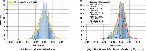
On the contrary, Figure 4(b) depicts that the distributions of the $\{1,2,5\}$ components of the GMM N_c = 5 model have tighter distributions, jointly gauging leptokurtic and asymmetric features of the empirical distribution. The distributions of the two remaining components are much flatter and approximate the tails. Hence, the combination of such distributions constructs a GM model that can better estimate the unevenness of the data distribution. These insights are in line with Tan (2005) who showed that by changing the mixture weights of components and other parameters, the GM model can better approximate various shapes of the data distributions compared to the normal, Cauchy, and Student distributions.

3.2. The evaluation of VaR based on GMM

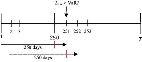
This subsection explains how to evaluate VaR using the GM model. First, we need to choose a period for the backtesting. The VaR model uses a 250-day rolling window method to calibrate and predict one-day maximum loss (Capital Requirements Regulation (575/2013) 2013; Basel Committee on Banking Supervision 2016). Then this value is compared with the historical loss. Later, a 250-day window is shifted forward by one day, and the described process repeats until the end of the backtesting interval is reached. The rolling window duration roughly uses one trading year for the initialization of VaR (see Figure 5). Hence, the operational sample size in the empirical part of the paper reduces by one year.

Figure 5. 250-day rolling window method.

For the estimation of the GM model parameters, the iterative Expectation Maximization (EM) algorithm is used instead of the maximum likelihood method, for which it is hard to optimize the log-likelihood function of GM distribution due to latent variables in the mixture model. In order to reduce computation time, instead of randomly selecting data points, the K-means⁵ algorithm is used to initialize the GM model parameters and then the EM algorithm optimizes them (see Figure 6).

Figure 6. The scheme of VaR evaluation based on the Gaussian Mixture Model.

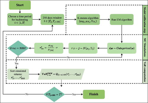
In the first step of the EM algorithm, the initial parameters are set to $({\omega }_i,{\mu }_i,{\mathrm{\Sigma }}_i),i=1,\dots ,N_c$, and then E and M steps are sequentially performed. The final step is to check the convergence of the log-likelihood function. If there is no convergence, the algorithm must repeat E and M steps.

1. E-step: estimate the posterior probabilities for each element: $$\begin{array}{l}p(z_i=k|x_i,{\theta }_t)={\displaystyle \frac{{\omega }_{k}f(x_i|{\mu }_k,{\mathrm{\Sigma }}_k)}{\sum _{j=1}^{N_c}{\omega }_{k}f(x_i|{\mu }_j,{\mathrm{\Sigma }}_j)}}=r_{\mathrm{ik}},k\in \{1,\dots ,N_c\}.\end{array}$$

2. M-step: update the parameters: $$\begin{array}{l}{\omega }_k={\displaystyle \frac{\sum _{i=1}^N{r}_{\mathrm{ik}}}{N}};{\mu }_k={\displaystyle \frac{\sum _{i=1}^N{r}_{\mathrm{ik}}{x}_i}{\sum _{i=1}^N{r}_{\mathrm{ik}}}}\text{ and }{\mathrm{\Sigma }}_k={\displaystyle \frac{\sum _{i=1}^N{r}_{\mathrm{ik}}(x_i-{\mu }_k)(x_i-{\mu }_k{)}^T}{\sum _{i=1}^N{r}_{\mathrm{ik}}}}.\end{array}$$

The next step of GMM-based VaR evaluation is to simulate latent variables z. The z = k value specifies which GMM component will generate the stock log-returns. Then obtained values multiplied by additional multiplier σ_[70]∕σ_[250]. The process repeats until the number of simulations (mc) reaches 3,000.

4. Backtesting methodology

VaR models are operational if they can assess potential losses with sufficient accuracy. Therefore, when applying these models in practice, it is always necessary to statistically evaluate whether they are fit and adequate for the available data.

Kupiec (1995) proposed the proportion of failures (PoF) test, which in this article used as described in Nieppola (2009). The PoF checks the null hypothesis that the proportion of failure—the ratio of exceptions⁶ (n) to the total number of observations (T) – is not significantly different from the chosen α level. The PoF statistic is defined as follows: $$\begin{array}{l}L{R}_{\mathrm{PoF}}=-2\ln [(1-\alpha {)}^{T-n}{\alpha }^n]-\ln \left[{(1-n/T)}^{T-n}{\left(n/T\right)}^n\right].\end{array}$$

If LR_PoF is greater than the critical value of the χ²(1) distribution, then the null hypothesis is rejected, meaning that the VaR model is not accurate enough.

Observed exceptions can be correlated and form exception clusters. Correlated losses can be extremely significant and large in a relatively short period of time. Christoffersen (1998) developed a test that evaluates not only the number of exceptions but also accounts for the dependence of losses on previous observations. However, Silva et al. (2006) noted that the test does not consider cases with more than one day between exceptions. If $L_t>{\text{VaR}}_{1-\alpha }$, where L_t is the loss at time t, then 𝟙_t = 1 indicates the appearance of exception, else 𝟙_t = 0. Let T_ij describe the number of days when the function 𝟙_t passed from the ith to the jth state (Jorion 2007). Besides, let π be the probability that an exception will occur, and π_i be the conditional probability that an exception will occur with the registration of ith event the day before: $$\begin{array}{l}{\pi }_0={\displaystyle \frac{T_{01}}{T_{00}+T_{01}}}={\displaystyle \frac{T_{01}}{T_{0\ast }}};{\pi }_1={\displaystyle \frac{T_{11}}{T_{10}+T_{11}}}={\displaystyle \frac{T_{11}}{T_{1\ast }}}\text{and}\pi ={\displaystyle \frac{T_{01}+T_{11}}{T_{00}+T_{01}+T_{10}+T_{11}}}={\displaystyle \frac{T_{\ast 1}}{T}}.\end{array}$$

Then, Christoffersen’s test statistic for evaluating the hypothesis that the exceptions are independent is: $$\begin{array}{l}L{R}_{\mathrm{ind}}=-2\ln [(1-\pi {)}^{T_{00}+T_{10}}{\pi }^{T_{01}+T_{11}}]+2\ln [(1-{\pi }_0{)}^{T_{00}}{\pi }_0^{T_{01}}(1-{\pi }_1{)}^{T_{10}}{\pi }_1^{T_{11}}],\end{array}$$ where the null hypothesis is rejected when LR_ind exceeds the critical value of the χ²(1) distribution.

The joint statistic, which takes into account both exception rates and their interdependence, is computed by adding the two defined above statistics – $L{R}_{\mathrm{CC}}=L{R}_{\mathrm{PoF}}+L{R}_{\mathrm{ind}}$, the null hypothesis of which is rejected when LR_CC is greater than the χ²(2) critical value.

The literature indicates that the probability of an exception today may not only depend on whether an exception occurred yesterday but may, for example, depend on an exception occurring one week ago (Campbell 2005). Haas (2001) introduced the Mixed Kupiec test, which estimates the number of exceptions and their dependence, taking into account that exceptions may depend on other exceptions that occurred more than a day ago: $$\begin{array}{l}L{R}_{\mathrm{mix}}=\sum _{i=2}^n-2\ln \left[{\displaystyle \frac{\alpha (1-\alpha {)}^{{\nu }_i-1}}{{\displaystyle \frac{1}{{\nu }_i}}{(1-{\displaystyle \frac{1}{{\nu }_i}})}^{{\nu }_i-1}}}\right]-2\ln \left[{\displaystyle \frac{\alpha (1-\alpha {)}^{\nu -1}}{{\displaystyle \frac{1}{\nu }}{(1-{\displaystyle \frac{1}{\nu }})}^{\nu -1}}}\right]+L{R}_{\mathrm{PoF}},\end{array}$$ where ν_i is the time between the ith and (i−1)th exception; ν is the time until the first exception. If LR_mix is greater than the χ²(n+1) critical value, then the null hypothesis is rejected and the VaR model is dynamically inaccurate.

5. Comparison of one-day VaR model predictions

This section presents a comparative analysis of the distinct VaR models’ predictions evaluated at the portfolio and individual stock levels in two disjoint periods. In the following tables, green color means that the statistical data does not contradict the test null hypothesis with p-value > 0. 01, i.e., null hypothesis cannot be rejected. Red color—the test null hypothesis is rejected. For GMM calculations, we use scikit-learn—a machine learning library that, among many other methods, includes a GMM function—mixture.GaussianMixture (scikit-learn developers 2017). High-performance computing (HPC) resources are used to perform the calculations⁷.

5.1. 2007–2010 period

This section reviews predictions for the period 2007–2010. For backtesting, each VaR method is evaluated 1,009 times using a 250-day rolling window method as defined in Section 3.2. According to the Basel II traffic light test specification⁸, during this validation period, the VaR₉₉ model is assigned to the green zone (i.e., the model is accurate) when the number of breaches is less than 16, the red zone (i.e., it is extremely likely model is inaccurate) starts at 24 breaches, otherwise—the yellow zone.

5.1.1. VaR model predictions of portfolio value

According to the number of failed tests, VaR₉₉ values are predicted the worst by VC and MC GBM methods (see Table 1). The number of exceptions for these approaches significantly exceeded 24 exceptions (i.e., Basel II test’s red zone). In addition, the results of the Kupiec test showed that the number of VaR exceptions is significantly different from the chosen model’s confidence level. But the Christoffersen test for these methods assessed that the exceptions are mutually independent, i.e., the probability that an exception will occur today is independent of what happened yesterday.

Table 1. The backtesting results (proportions of passed tests) of stock VaR estimates, 2007–2010.

Approach	Median no. of breaches	Kupiec	Christoffersen	Joint test	Mixed Kupiec
GMM Nc = 3	15	96.39	97.60*	93.27	48.08
GMM Nc = 4	15	97.06	97.36	94.95*	49.76
GMM Nc = 5	14*	97.36*	97.36	93.75	50.72*
Variance-covariance (VC)	18	69.95	96.63	64.42	24.52
Monte-Carlo (MC) GBM	19	66.35	95.67	62.02	24.76
Historical	17	89.42	97.12	84.62	32.93

*The text is bold for the best results, defined as the smallest median number of breaches and the largest proportion of passed tests.

It has been found that a GMM with N_c = 5 method is the best fit for the available data. This method resulted in the smallest number of model breaches and passed four out of five backtesting tests with relatively high p-values. However, GMM N_c = 5 and other VaR methods result in dependent exceptions when the difference between them is longer than one day, as in all cases, the null hypothesis of the Mixed Kupiec test is rejected. Despite the smallest number of exceptions, the obtained BIC values show that GMM N_c = 3 is the preferred method for the current data compared to other GMM methods. Accordingly, the BIC measure alone does not suffice to select the most suitable model. In addition, backtesting procedures should be conducted to make sure that the model is selected properly.

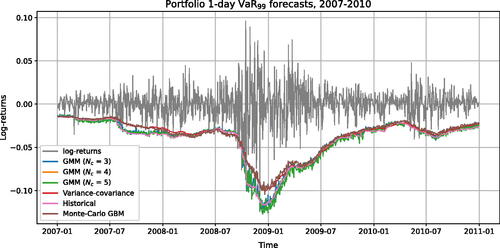
In the calmer time periods of 2007–2010, all methods predicted relatively similar VaR values (see Figure 7). However, on September 15, 2008, a “black swan” occurred—one of the largest US investment banks, Lehman Brothers, declared bankruptcy, after which market volatility increased rapidly. It is apparent that all VaR approaches provide a delayed response to such an event. However, GMM and Historical methods showed a faster response, while the remaining traditional methods were insufficiently conservative. During the crisis, the GMM machine learning approaches proactively redistribute the mixture weights based on significant recent changes in the data, leading to a higher prediction rate of negative stock returns and the lowest number of model breaches. After stock market stabilization, the additional volatility multiplier helps all VaR methods rapidly revert to pre-crisis levels, preventing them from predicting too conservative VaR values. Furthermore, it is evident that GMM methods provide more fluctuating VaR predictions than other methods. However, the formula for market risk capital requirements in the Basel III framework involves a 60-day average of 10-day VaR and 10-day Stressed VaR. Therefore, regulatory capital requirements based on GMM VaR methods will be smoother and more stable than single one-day VaR predictions.

Figure 7. VaR₉₉ forecasts for a portfolio value (PV), 2007–2010.

5.1.2. VaR model predictions for individual stocks

The individual stock level shares its aggregate—the portfolio level—differences discussed above. Table 2 provides the proportions of passed tests estimated by running each backtesting test for all analyzed stocks. A comparison of VC and MC GBM with other methods shows that they have the lowest proportion of passed tests across all backtesting tests. This indicates that these approaches often tend to underestimate VaR measures, resulting in an excessive number of model breaches that are also not independent. This striking similarity between the methods originates from the fact that both approaches rely on the normality assumption. A promising exclusion among traditional methods is the Historical approach, but GM models have higher proportions of passed tests. GM model with N_c = 5 is the most suitable method for most stock data because it exhibits the highest passing rates for Kupiec and Mixed Kupiec tests and has the smallest median number of model breaches; other GMMs come in second—overall differences are relatively small.

Table 2. The backtesting results (proportions of passed tests) of stock VaR estimates, 2017–2021.

Approach	Median no. of breaches	Kupiec	Christoffersen	Joint test	Mixed Kupiec
GMM Nc = 3	19	89.66	87.74	77.16	20.19
GMM Nc = 4	19	90.38*	88.46*	78.85	19.23
GMM Nc = 5	19	90.38*	87.02	79.57*	20.67*
Variance-covariance (VC)	29	10.82	77.88	10.34	0.96
Monte-Carlo (MC) GBM	30	9.13	77.4	6.49	1.20
Historical	22	68.27	86.78	56.73	10.58

*The text is bold for the best results, defined as the smallest median number of breaches and the largest proportion of passed tests.

The histograms in Figure 8 summarize the information regarding the distribution of recorded breaches for the different VaR methods that were estimated separately for each stock. The comparison shows that the VC and MC GBM VaR methods differ from other approaches, having distributions of model exceptions considerably shifted to the right side from the green zone and being flatter than for other approaches, indicating that the normality assumption based methods more often underestimate VaR measures.

Figure 8. Number of breaches for different individual stock VaR models, 2007–2010.

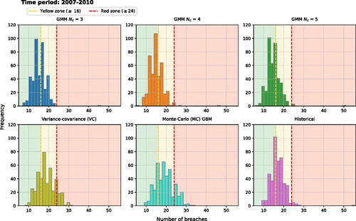
At first glance, the breach data shape seems to be similar among the GMM and Historical VaR approaches. A closer look reveals that the Historical method is characterized by a heavier right tail accompanied by an outlier representing 55 breaches. Contrary to this, GMM methods have significantly lighter right tails, with one outlier value of less than 50 model exceptions. Additionally, the Kolmogorov-Smirnov (KS) test is applied to evaluate whether breach data distributions statistically differ. Thus, there is no statistically significant difference in the distribution of breach data across the GMM methods and the pair of VC and MC GBM approaches, while distinctions for the other pairs are significant. Moreover, the GMM methods have a higher frequency of model breaches near the green zone area. It corresponds with the high proportions of passed Kupiec tests (i.e., more than 96%), while VC, MC GBM have up to 70% and Historical have 89%.

5.2. 2017–2021 period

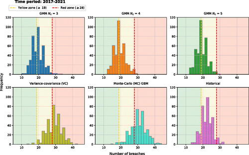
This section reviews predictions for the period 2017–2021. For backtesting, each method is evaluated 1,261 times using a 250-day rolling window method as defined in Section 3.2. Based on the Basel II traffic light test⁸, during this validation period, the VaR₉₉ model is considered an adequate model (green zone) when the quantity of model breaches is less than 19, red zone—greater or equal to 28 breaches.

5.2.1. VaR model predictions of portfolio value

In the pandemic period, VC and MC GBM methods based on normality assumptions again performed the worst (see Table 3). MC GBM among the two, is the most suboptimal way of calculating VaR for different confidence levels, having numerous dependent exceptions significantly exceeding the acceptable level. Meanwhile, the historical approach is the best method for the available data, resulting in 17 model breaches and passing two out of five tests. This is the only case in which the historical method outperformed the GMM methods. The GMM N_c = 4 is judged to be the second most fitting VaR₉₉ method for the available data with 20 exceptions when the rest of GMM have 21 and 24 exceptions. Again, it is observed that the minimum BIC value has a model that does not have the least number of exceptions. Although the GMM N_c = 3 method has the lowest BIC estimate, it produced a significantly larger number of exceptions than the GMM N_c = 4 method, which has a higher BIC estimate.

Table 3. The backtesting results (p-values) of portfolio VaR estimates, 2017–2021.

Approach	No. of breaches	Basel II	Kupiec	Christoffersen	Joint test	Mixed Kupiec
GMM Nc = 3 (BIC = 408 550)	24	PASS	0.000	0.009	0.001	0.000
GMM Nc = 4 (BIC = 858 106)	20	PASS	0.050	0.003	0.002	0.000
GMM Nc = 5 (BIC = 1 316 484)	21	PASS	0.030	0.004	0.001	0.000
Variance-covariance (VC)	33	FAIL	0.000	0.001	0.000	0.000
Monte-Carlo (MC) GBM	36	FAIL	0.000	0.003	0.000	0.000
Historical	17	PASS	0.230	0.001	0.002	0.000

Figure 9 shows that all VaR methods combined with an additional volatility multiplier can maintain the characteristics observed in the previous period, i.e., faster adaption to rapidly changed market conditions and more accurate VaR predictions. But among the other approaches, the VC and MC GBM methods appear to underestimate losses significantly more often than the others.

Figure 9. VaR₉₉ forecasts for a portfolio value (PV), 2017–2021.

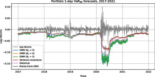
However, despite the advantages of the additional historical volatility multiplier, it is clear that none of the VaR approaches is a panacea when a “black swan” appears in the market. In this period, the “black swan” event corresponds to the sharp stock market fluctuations observed between February and March 2020. It is evident that before this event, the market volatility had calmed, so even with a volatility multiplier, it was impossible to anticipate such sudden and substantial changes using just historical data.

Additionally, one-day VaR predictions were compared across different methods during the relatively stable 2017–2019 period, preceding the COVID-19 pandemic (see Table A.1). The outcomes closely resemble our previous results, with both the GMM N_c = 5 and the Historical method demonstrating similar performance by successfully passing all backtesting tests.

5.2.2. VaR model predictions for individual stocks

Likewise, portfolio level, due to the specifics of the 2017–2021 period, the Mixed Kupiec test was usually not passed at the stock level (see Table 4). Similarly to the previous period, GMMs remained the VaR methods with the highest rate of passed tests. However, only a small fraction of individual stocks have also passed the Mixed Kupiec test, yet significant to conclude that the passing rate is higher than just random observation—a fact not refuted for normality based VC and MC approaches.

Table 4. The backtesting results (proportions of passed tests) of stock VaR estimates, 2017–2021.

Approach	edian no. of breaches	Kupiec	Christoffersen	Joint test	Mixed Kupiec
GMM Nc = 3	19	89.66	87.74	77.16	20.19
GMM Nc = 4	19	90.38*	88.46*	78.85	19.23
GMM Nc = 5	19	90.38*	87.02	79.57*	20.67*
Variance-covariance (VC)	29	10.82	77.88	10.34	0.96
Monte-Carlo (MC) GBM	30	9.13	77.4	6.49	1.20
Historical	22	68.27	86.78	56.73	10.58

*The text is bold for the best results, defined as the smallest median number of breaches and the largest proportion of passed tests.

Noteworthy, the Historical method also often passed 3 out of 4 tests for most stocks, and the numbers of exceptions are comparable to those of the GMM methods that follow analysing the histograms summarized in Figure 10. The VC and MC GBM remained the most suboptimal VaR calculation methods with flatter and significantly shifted to the red zone distribution of the number of breaches. There is a high concentration of breaches in the yellow zone for the historical method, whereas the breach distribution across green and yellow zones appears to be nearly equal in the GMM approaches. Furthermore, the KS test failed to reject the null hypothesis of similar distributions only for pairs of GMM methods.

Figure 10. Number of breaches for different individual stock VaR models, 2017–2021.

Summarizing Section 5, a comparable analysis is performed because the σ_[70]∕σ_[250] multiplier is applied to both GMM and traditional VaR methods with a focus on the latter methods as these, to our knowledge, were not previously used with flexibility increasing multiplier. In this regard, traditional VaR methods are compiled for the portfolio and individual stocks without using an additional volatility multiplier to evaluate its impact on the accuracy of one-day VaR predictions. The following plots in Figure 11 (see supplementary Figure A.1) illustrate the main idea of σ_[70]∕σ_[250] multipliers—faster adaptation to changing market conditions. VaR forecasts with additional volatility multipliers derived from historical data do not lag behind the dominating market state. When higher volatility occurs, VaR predictions become more conservative, capturing the portfolio’s risk more effectively. Otherwise, when market conditions return to more stable ones, the forecasts adjust and become less conservative, preventing inefficient use of capital.

Figure 11. Volatility σ_[70]∕σ_[250] ratio’s effect on portfolio VC VaR, 2007–2010 and 2017–2021.

Furthermore, in the “black swan” event of a financial crisis, VaR predictions without a multiplier increased only after more than a half year, except for the historical method, which showed slightly faster adaptation. In the wake of another “black swan” of the COVID-19 pandemic, similar trends are observed. Backtesting tests are generally improved by the addition of a volatility multiplier because it decreases the number of breaches. However, there are some cases where this property does not hold. With the addition of the volatility multiplier, the number of model exceptions is moderately increased for MC GBM stock VaR and historical portfolio VaR in the period from 2017 to 2021 (see Tables A.2 and A.3). There might be several factors contributing to this, including the number of Monte-Carlo simulations used or the characteristics of the multiplier that is selected. Nevertheless, this additional multiplier improves accuracy and performance, while at the same time fulfilling the main regulatory requirements of a VaR model calibration based on at least one year (approximately 250 days) of historical observations.

6. Conclusions

Primary data analysis of the 2006–2010 and 2016–2021 periods showed that the distribution of stock log-returns is statistically significantly different from Gaussian. In the first period, the empirical standard deviations of stock log-returns are significantly higher, and all stock pairs have positive correlations, while in 2016–2021, there are some negative correlations.

The theoretical part of the article presents the Gaussian Mixture Model and reveals its several important statistical properties. Graphical and statistical analysis showed that the probability densities of the analyzed stock log-returns are unimodal. Therefore, a sufficient condition is formulated when the probability density of a GM distribution consisting of two components is unimodal. Additionally, the conditions are described when the tails of the GM distribution can be heavier than the tails of a single normal distribution. However, this property does not hold if the standard deviations of both GM component distributions are less than the estimate of the standard deviation of a single normal distribution.

According to the evaluation of the accuracy of VaR predictions, none of the methods can predict “black swan” events. However, the GMM method, by fine-tuning the weights of the mixture and using the standard deviation multiplier, can adapt to the changed market conditions more quickly, which results in a more accurate assessment of risks and a reduction in the number of VaR model exceptions. Therefore, the GMM approach is judged to be the most appropriate approach for the analyzed data.

A fair comparison and proposal is, hence, to equip the other approaches with the same multiplier that, to our knowledge, was not previously considered in the literature. In this regard, GMM is the most effective, followed by the Historical method. We conclude that Variance-Covariance and Monte-Carlo GBM methods based on normality assumptions are among the least preferable VaR approaches. They underestimate VaR values and fail to properly reflect the changes in risk factors, implying correlated model exceptions.

In addition, it is observed that the GMM could be an additional tool to indicate when the market is operating in conditions of increased or, on the contrary, decreased volatility. These signals can derive from changes in the weight of the mixture. It is just a matter of finding out what market condition each component describes. In addition, it is crucial that such an assignment makes economic sense. The analysis can provide additional information when analyzing the causes of exceptions in internal VaR models and may lead to more informed investment decisions without applying any other VaR approaches.

In order to further investigate the applicability of GMM in market risk management, it is necessary to examine the statistical properties of a finite number of components rather than a two-component model. However, the derivation of these properties will be more technical. It is also crucial to derive the necessary and sufficient conditions for the density of the GM distribution to be unimodal. Furthermore, considering the transition to the new Basel regulations for market risk, the GMM method can be tested for evaluating Expected Shortfall (ES). Also, it would be beneficial to investigate the ability of GMM methods to predict VaR or ES values when the portfolio includes more complex financial instruments, such as bonds or options, and to explore working with more diversified portfolios similar to those studied by Fama and French (1993).

Moreover, the consideration of heavy-tailed distributions is important for robust risk management, particularly in capturing tail risk adequately. The methodologies proposed by Beran et al. (2014), Jordanova et al. (2016), and Figueiredo et al. (2017) explain the estimation of tail behavior and provide valuable insights into tail index estimation, offering improved accuracy and robustness. Including heavy-tails-directed VaR developments into our analysis could further increase the effectiveness of risk assessment, particularly in identifying extreme “black swan” events and tail risk. By incorporating methodologies like the t-Hill estimator, harmonic moment tail index estimator (HME), and the PORT−MO_p VaR estimator, along with other Extreme Value Theory (EVT) models, can better understand and quantify tail risk in financial portfolios. Therefore, future research could focus on combining these advanced tail estimation approaches with the VaR framework, potentially leading to more accurate and reliable risk measures, especially in cases of heavy-tailed distributions.

Disclosure statement

No potential conflict of interest was reported by the author(s).

Notes

1. Data source—“YahooFinance” (link: https://finance.yahoo.com/).

3. $\mathrm{JB}=N/6({\gamma }_1^2+({\gamma }_2-3{)}^2/4)$ is Jarque-Bera test metric, where γ₁ is skewness and γ₂ – kurtosis coefficients.

4. HDS test is applied for 250 day rolling time window (2006–2010 and 2016–2021). Therefore, hypotheses are tested based on the averages of the obtained p-values.

5. More information about the K-means algorithm can be found in works of MacQueen (1967) and Raschka (2015).

6. Exception is the case when the loss exceeds the estimated value of the VaR model (i.e., $L_{t+1}>$ VaR${}_{1-\alpha }^t$).

7. The authors are thankful for the HPC resources provided by the Information Technology Research Center of Vilnius University.

8. Yellow zone begins at a point at which the binomial probability of achieving that number or fewer breaches equals or exceeds 95% confidence level, and red zone—at a point where the probability equals or exceeds 99.99% (Basel Committee on Banking Supervision 1996).

Appendix

Appendix

A.1. Proof of Lemma 3.1

Proof.

Assume that σ₁≠σ₂ and μ₁ < μ₂. Since x = μ₁ is not a root of $p^{\prime }(x,\omega )=\{\mathrm{\omega f}(x|{\mu }_1,{\sigma }_1)+$ $(1-\omega )f(x|{\mu }_2,{\sigma }_2){\}}^{\prime }=0$, this equality can be divided by the first component of p^′(x, ω) derivative function. Then: $$\begin{array}{l}g(x,\omega )={\displaystyle \frac{p^{\prime }(x,\omega )}{A}}={\displaystyle \frac{{\mu }_2-x}{x-{\mu }_1}}h(x)={\displaystyle \frac{\omega {\sigma }_2^3}{(1-\omega ){\sigma }_1^3}},\end{array}$$ where $A={\displaystyle \frac{-\omega (x-{\mu }_1)}{{\sigma }_1^3\sqrt{2\pi }}}\exp \{-{\displaystyle \frac{(x-{\mu }_1{)}^2}{2{\sigma }_1^2}}\}$ and $h(x)=\exp \{-{\displaystyle \frac{(x-{\mu }_2{)}^2}{2{\sigma }_2^2}}+{\displaystyle \frac{(x-{\mu }_1{)}^2}{2{\sigma }_1^2}}\}$.

Function g(x, ω) is positive only in ${\mu }_1<x<{\mu }_2$. Moreover, it is continuous function because $g(x,\omega )\to 0,\text{when }x\to {\mu }_1,{\mu }_2$. The function g(x, ω) will uniquely map all positive values if it is monotonically decreasing (i.e., $g^{\prime }(x,\omega )<0$, when ${\mu }_1<x<{\mu }_2$): (A.1) $$\begin{array}{ll}{g}^{\prime }(x,\omega )& ={({\displaystyle \frac{{\mu }_2-x}{x-{\mu }_1}}h(x))}^{\prime }={\left({\displaystyle \frac{{\mu }_2-x}{x-{\mu }_1}}\right)}^{\prime }h(x)+\left({\displaystyle \frac{{\mu }_2-x}{x-{\mu }_1}}\right)h^{\prime }(x)\\ & ={\displaystyle \frac{h(x)}{{\sigma }_1^2{\sigma }_2^2(x-{\mu }_1{)}^2}}(-({\mu }_2-{\mu }_1){\sigma }_2^2{\sigma }_1^2+({\mu }_2-x{)}^2(x-{\mu }_1){\sigma }_1^2+({\mu }_2-x)(x-{\mu }_1{)}^2{\sigma }_2^2)\\ & <{\displaystyle \frac{h(x)}{{\sigma }_1^2{\sigma }_2^2(x-{\mu }_1{)}^2}}({\displaystyle \frac{4}{27}}({\sigma }_1^2+{\sigma }_2^2)({\mu }_2-{\mu }_1{)}^3-{\sigma }_1^2{\sigma }_2^2({\mu }_2-{\mu }_1)).\end{array}$$(A.1)

Thus, $g^{\prime }(x,\omega )<0$ only when: (A.2) $$\begin{array}{l}{\displaystyle \frac{4}{27}}({\sigma }_1^2+{\sigma }_2^2)({\mu }_2-{\mu }_1{)}^3-{\sigma }_1^2{\sigma }_2^2({\mu }_2-{\mu }_1)<0\Rightarrow ({\mu }_2-{\mu }_1{)}^2<{\displaystyle \frac{27{\sigma }_1^2{\sigma }_2^2}{4({\sigma }_1^2+{\sigma }_2^2)}}.\end{array}$$(A.2)

This proves that with all ω and ${\mu }_1,{\mu }_2,{\sigma }_1,{\sigma }_2$ which satisfies (A.2(A.2) $$\begin{array}{l}{\displaystyle \frac{4}{27}}({\sigma }_1^2+{\sigma }_2^2)({\mu }_2-{\mu }_1{)}^3-{\sigma }_1^2{\sigma }_2^2({\mu }_2-{\mu }_1)<0\Rightarrow ({\mu }_2-{\mu }_1{)}^2<{\displaystyle \frac{27{\sigma }_1^2{\sigma }_2^2}{4({\sigma }_1^2+{\sigma }_2^2)}}.\end{array}$$(A.2) ) inequality, there is only one x value such that $p^{\prime }(x,\omega )=0$. Moreover, it will have a maximum value since $p(x,\omega )\to 0$ when $x\to \pm \mathrm{\infty }$. However, this inequality is only a sufficient condition for unimodality of GM distribution for all $\omega ,0<\omega <1$.

Below is the additional proof of (A.1(A.1) $$\begin{array}{ll}{g}^{\prime }(x,\omega )& ={({\displaystyle \frac{{\mu }_2-x}{x-{\mu }_1}}h(x))}^{\prime }={\left({\displaystyle \frac{{\mu }_2-x}{x-{\mu }_1}}\right)}^{\prime }h(x)+\left({\displaystyle \frac{{\mu }_2-x}{x-{\mu }_1}}\right)h^{\prime }(x)\\ & ={\displaystyle \frac{h(x)}{{\sigma }_1^2{\sigma }_2^2(x-{\mu }_1{)}^2}}(-({\mu }_2-{\mu }_1){\sigma }_2^2{\sigma }_1^2+({\mu }_2-x{)}^2(x-{\mu }_1){\sigma }_1^2+({\mu }_2-x)(x-{\mu }_1{)}^2{\sigma }_2^2)\\ & <{\displaystyle \frac{h(x)}{{\sigma }_1^2{\sigma }_2^2(x-{\mu }_1{)}^2}}({\displaystyle \frac{4}{27}}({\sigma }_1^2+{\sigma }_2^2)({\mu }_2-{\mu }_1{)}^3-{\sigma }_1^2{\sigma }_2^2({\mu }_2-{\mu }_1)).\end{array}$$(A.1) ) inequality because Eisenberger (1964) proposed it in his paper without theoretical justification: $$\begin{array}{l}({\mu }_2-x{)}^2(x-{\mu }_1){\sigma }_1^2+({\mu }_2-x)(x-{\mu }_1{)}^2{\sigma }_2^2\le {\displaystyle \frac{4}{27}}({\sigma }_1^2+{\sigma }_2^2)({\mu }_2-{\mu }_1{)}^3.\end{array}$$

To prove (A.1(A.1) $$\begin{array}{ll}{g}^{\prime }(x,\omega )& ={({\displaystyle \frac{{\mu }_2-x}{x-{\mu }_1}}h(x))}^{\prime }={\left({\displaystyle \frac{{\mu }_2-x}{x-{\mu }_1}}\right)}^{\prime }h(x)+\left({\displaystyle \frac{{\mu }_2-x}{x-{\mu }_1}}\right)h^{\prime }(x)\\ & ={\displaystyle \frac{h(x)}{{\sigma }_1^2{\sigma }_2^2(x-{\mu }_1{)}^2}}(-({\mu }_2-{\mu }_1){\sigma }_2^2{\sigma }_1^2+({\mu }_2-x{)}^2(x-{\mu }_1){\sigma }_1^2+({\mu }_2-x)(x-{\mu }_1{)}^2{\sigma }_2^2)\\ & <{\displaystyle \frac{h(x)}{{\sigma }_1^2{\sigma }_2^2(x-{\mu }_1{)}^2}}({\displaystyle \frac{4}{27}}({\sigma }_1^2+{\sigma }_2^2)({\mu }_2-{\mu }_1{)}^3-{\sigma }_1^2{\sigma }_2^2({\mu }_2-{\mu }_1)).\end{array}$$(A.1) ) inequality, it only remains to verify that the following inequalities are satisfied: (A.3) $$\begin{array}{l}({\mu }_2-x{)}^2(x-{\mu }_1)\le {\displaystyle \frac{4}{27}}({\mu }_2-{\mu }_1{)}^3\text{ and }({\mu }_2-x)(x-{\mu }_1{)}^2\le {\displaystyle \frac{4}{27}}({\mu }_2-{\mu }_1{)}^3.\end{array}$$(A.3)

Let $f(x):=({\mu }_2-x{)}^2(x-{\mu }_1)=x^3-({\mu }_1+2{\mu }_2)x^2+({\mu }_2^2+2{\mu }_1{\mu }_2)x-{\mu }_1{\mu }_2^2.$

From f^′(x) = 0 follows that f(x) function in (μ₁, μ₂) has maximum at point of $x_1=(2{\mu }_1+{\mu }_2)/3$ because f^′′(x₁) < 0. Then we insert x₁ expression into f(x = x₁) to show that: $$\begin{array}{ll}f(x={\displaystyle \frac{2{\mu }_1+{\mu }_2}{3}})& ={({\mu }_2-{\displaystyle \frac{2{\mu }_1+{\mu }_2}{3}})}^2({\displaystyle \frac{2{\mu }_1+{\mu }_2}{3}}-{\mu }_1)\\ & ={\displaystyle \frac{4}{27}}({\mu }_2-{\mu }_1{)}^2\le {\displaystyle \frac{4}{27}}({\mu }_2-{\mu }_1{)}^2.\end{array}$$

Likewise, show that $f(x):=({\mu }_2-x)(x-{\mu }_1{)}^2=-x^3+({\mu }_2+2{\mu }_1)x^2-(2{\mu }_2{\mu }_1-{\mu }_1^2)x+{\mu }_2{\mu }_1^2$ function attains maximum at point of $x_2=(2{\mu }_2+{\mu }_1)/3$ and f(x = x₂) expression shows that (A.3(A.3) $$\begin{array}{l}({\mu }_2-x{)}^2(x-{\mu }_1)\le {\displaystyle \frac{4}{27}}({\mu }_2-{\mu }_1{)}^3\text{ and }({\mu }_2-x)(x-{\mu }_1{)}^2\le {\displaystyle \frac{4}{27}}({\mu }_2-{\mu }_1{)}^3.\end{array}$$(A.3) ) inequalities are satisfied. ▪

A.2. One-day VaR model predictions, 2017–2019 period

One-day VaR predictions are presented for 2017–2019 (in total of 759 observations), along with applied backtesting tests. These evaluations were conducted during a comparatively tranquil period before the emergence of the COVID-19 pandemic to assess the performance of different methods under conditions of lower volatility (Table A.1).

A.3. Volatility ratio’s effect on traditional VaRmethods

Table A.1. The backtesting results (p-values) of portfolio VaR estimates, 2017–2019 (759 observations).

Approach	No. of breaches	Basel II	Kupiec	Christoffersen	Joint test	Mixed Kupiec
GMM Nc = 3	11	PASS	0.240	0.146	0.173	0.005
GMM Nc = 4	10	PASS	0.400	0.116	0.203	0.019
GMM Nc = 5	9	PASS	0.610	0.091	0.210	0.026
Variance-covariance (VC)	18	PASS	0.000	0.007	0.000	0.000
Monte-Carlo (MC) GBM	19	PASS	0.000	0.010	0.000	0.000
Historical	8	PASS	0.870	0.068	0.187	0.023

Table A.2. Stocks VaR with and without volatility multiplier, 2007–2010 and 2017–2021.

Approach	Period	σ[70]/σ[250] ratio	Average no. of breaches	Kupiec	Christoffersen	Joint test	Mixed Kupiec
Variance-covariance (VC)	2007–2010	added	19	69.95	96.63	64.42	24.52
		removed	23	33.41	87.02	28.37	5.77
	2017–2021	added	29	10.82	77.88	10.34	0.96
		removed	27	25.24	63.46	17.31	1.20
Monte-Carlo (MC) GBM	2007–2010	added	19	66.35	95.67	62.02	24.76
		removed	24	32.93	89.66	27.16	6.49
	2017–2021	added	30	9.13	77.40	6.49	1.20
		removed	28	17.79	60.34	12.5	0.72
Historical	2007–2010	added	17	89.42	97.12	84.62	32.93
		removed	20	56.97	89.90	45.91	8.65
	2017–2021	added	22	68.27	86.78	56.73	10.58
		removed	20	91.11	66.35	59.13	5.53

Table A.3. Portfolio VaR with and without volatility multiplier, 2007–2010 and 2017–2021.

		σ[70]∕σ[250]	No. of			Joint	Mixed
Approach	Period	ratio	breaches	Kupiec	Christoffersen	test	Kupiec
Variance-covariance (VC)	2007–2010	added	33	0.000	0.135	0.000	0.000
		removed	38	0.000	0.691	0.000	0.000
	2017–2021	added	33	0.000	0.001	0.000	0.000
		removed	37	0.000	0.004	0.000	0.000
Monte-Carlo (MC) GBM	2007–2010	added	31	0.000	0.160	0.000	0.000
		removed	40	0.000	0.602	0.000	0.000
	2017–2021	added	36	0.000	0.003	0.000	0.000
		removed	38	0.000	0.005	0.000	0.000
Historical	2007–2010	added	16	0.080	0.472	0.172	0.000
		removed	31	0.000	0.160	0.000	0.000
	2017–2021	added	17	0.230	0.001	0.002	0.000
		removed	16	0.350	0.001	0.002	0.000

Figure A.1. Volatility σ_[70]∕σ_[250] ratio’s effect on traditional portfolio VaR measures, 2007–2010 and 2017–2021.

References

- Adams M, Thornton B. 2013. Black swans and VaR. J Financ Acc. 14:1–17.
- Basel Committee on Banking Supervision 1996. Supervisory framework for the use of “Backtesting” in conjunction with the internal models approach to market risk capital requirements. Basel Committee on Banking Supervision, https://www.bis.org/publ/bcbs22.pdf.
- Basel Committee on Banking Supervision 2016. Minimum capital requirements for market risk. Basel Committee on Banking Supervision, https://www.bis.org/bcbs/publ/d352.pdf?fbclid=IwAR3ttD8Rda4FcyhZwDVnYJ9fsNw6wKOhcciMBk5BOcEyIh3p0GRmDEUuAMo#
- Beran J, Schell D, Stehlík M. 2014. The harmonic moment tail index estimator: asymptotic distribution and robustness. Ann Inst Stat Math. 66:193–220. doi:10.1007/s10463-013-0412-2.
- Campbell SD. 2005. A review of backtesting and backtesting procedures. FEDS. 2005:1–23. doi:10.17016/FEDS.2005.21.
- Capital Requirements Regulation 2013. Article 365: VaR and stressed VaR calculation. Capital Requirements Regulation (575/2013), https://eur-lex.europa.eu/legal-content/EN/TXT/?uri=celex:32013R0575.
- Christoffersen PF. 1998. Evaluating interval forecasts. Int Econ Rev. 39:841. doi:10.2307/2527341.
- Contreras RJ. 2014. Market risk measures using finite gaussian mixtures. J Appl Finan Bank. 4:29–45.
- Cox, J. 2021. Investors have put more money into stocks in the last 5 months than the previous 12 years combined. https://www.cnbc.com/2021/04/09/investors-have-put-more-money-into-stocks-in-the-last-5-months-than-the-previous-12-years-combined.html.
- Cox, J. 2022. Inflation surges 7.5% on an annual basis, even more than expected and highest since 1982. https://www.cnbc.com/2022/02/10/january-2022-cpi-inflation-rises-7point5percent-over-the-past-year-even-more-than-expected.html.
- Cuevas-Covarrubias C, Inigo-Martinez J, Jimenez-Padilla R. 2017. Gaussian mixtures and financial returns. Discuss Math Probab Stat. 37:101. doi:10.7151/dmps.1190.
- Dey, E, 2022. S&P 500 plunges to nine-month low as Russia invades Ukraine. https://www.bloomberg.com/news/articles/2022-02-24/s-p-500-plunges-to-nine-month-low-as-russia-invades-ukraine.
- Eisenberger I. 1964. Genesis of bimodal distributions. Technometrics. 6:357–363. doi:10.1080/00401706.1964.10490199.
- Fama EF, French KR. 1993. Common risk factors in the returns on stocks and bonds. J Financ Econ. 33:3–56. doi:10.1016/0304-405X(93)90023-5.
- Feller, W. 1968. The normal approximation to the binomial distribution. In: An introduction to probability theory and its applications. Vol. 1 New York: Wiley. p. 174–196.
- Figueiredo F, Gomes M, Rodrigues L. 2017. Value-at-risk estimation and the port mean-of-order-p methodology. Revstat- Stat J. 15:187–204.
- Haas, M. 2001. New methods in backtesting. https://www.ime.usp.br/rvicente/risco/haas.pdf.
- Hartigan AJ, Hartigan MP. 1985. The Dip test of unimodality. Ann Stat. 13:70–84.
- Hull, JC. 2015. London: Pearson education. Value at risk. In: Options, futures, and other derivatives 9th ed., 494–520.
- Jordanova P, Fabián Z, Hermann P, Střelec L, Rivera A, Girard S, Torres S, Stehlík M. 2016. Weak properties and robustness of t-Hill estimators. Extremes. 19:591–626. doi:10.1007/s10687-016-0256-2.
- Jorion, P. 2007. Backtesting VaR. In: Value at risk: the new benchmark for managing financial risk, 3rd ed.New York: McGraw-Hill. p. 153–158.
- Kupiec PH. 1995. Techniques for verifying the accuracy of risk measurement models. JOD. 3:73–84. doi:10.3905/jod.1995.407942.
- Macqueen, J. 1967. Some methods for classification and analysis of multivariate observations. Proc Fifth Berkeley Symp Math Statist Prob. 1:281– 297.
- Mandelbrot B. 1963. The variation of certain speculative prices. J BUS. 36:394. doi:10.1086/294632.
- Markowitz H. 1952. Portfolio selection*. J Finance. 7:77–91. doi:10.1111/j.1540-6261.1952.tb01525.x.
- Morgan, JP. 1996. RiskMetrics technical document. https://www.msci.com/documents/10199/5915b101-4206-4ba0-aee2-3449d5c7e95a.
- Nieppola, O. 2009. Backtestig Value-at-Risk Models. Master’s Thesis, Helsinki School of Economics. https://aaltodoc.aalto.fi/server/api/core/bitstreams/fafacabc-c1c0-4e52-b2f3-35dd99d03e71/content.
- Raschka, S. 2015. Working with unlabeled data-clustering analysis. In: Python machine learning. Birmingham: Packt Publishing, p. 311–340.
- Rudin C. 2021. Gaussian mixture models and expectation maximization. https://users.cs.duke.edu/cynthia/teaching.html.
- Sarkar D., Bali R., Sharma T. 2018. Backtesting VaR. In: Practical machine learning with Python: a problem-solver’s guide to building real-world intelligent systems. Berkeley (CA): Apress, p. 38–42.
- scikit-learn developers. 2017. scikit-learn user guide 0.18.2. https://scikit-learn.org/0.18/_downloads/scikit-learn-docs.pdf.
- Seyfi SMS, Sharifi A, Arian H. 2021. Portfolio Value-at-Risk and expected-shortfall using an efficient simulation approach based on Gaussian Mixture Model. Math Comput Simul. 190:1056–1079. doi:10.1016/j.matcom.2021.05.029.
- Silva RCA, Da Silveira Barbedo CH, Araújo GS, Das Neves, MBE. 2006. Internal models validation in Brazil: analysis of VaR backtesting methodologies, https://www.redalyc.org/articulo.oa?id=305824716005.
- Taleb, NN. 2008. The Black Swan: the impact of the highly improbable. New York: Random House.
- Tan K. 2005. Modeling returns distribution based upon radical normal distributions. J Soc Stud Ind Econ. 46:371–383.
- Tan K, Chu M. 2012. Estimation of portfolio return and value at risk using a class of Gaussian mixture distributions. Int J Bus Finance Res. 6:97–107.
- Tan K, Tokinaga S. 2007. Approximating probability distribution function based upon mixture distribution optimized by genetic algorithm and its application to tail distribution analysis using importance sampling method. J Polit Econ. 74:183–196.
- Wang Z, Ritou M, Da Cunha C, Furet B. 2020. Contextual classification for smart machining based on unsupervised machine learning by Gaussian mixture model. Int J Comput Integr Manuf. 33:1042–1054. doi:10.1080/0951192X.2020.1775302.