Assessing temporary product-specific subsidies: a time series intervention analysis

Abstract.

We propose an analytical forecasting framework to quantify the distortionary effects of product-specific subsidies. The novelty consists of a dual approach combining intervention analysis and a state-space modeling approach to construct and assess counterfactuals. Our pure intervention model approach faces challenges in identifying policy effects because, in certain sectors, these are weak and align with the crisis. We complement this approach by fitting a bivariate state-space model excluding the policy and creating counterfactual forecasts for periods of crisis. We then compare intervention analysis estimates of counterfactual series to those of observed series. Subsidizing one industry during global recessions seems unjustified and non-competitive. In our application, we use a time series of foreign and domestic order book levels during and after the temporary installation of an unprecedentedly generous car scrappage scheme in 2009. We assess implied disruptions in the automobile sector and eleven competing manufacturing industries in Germany. We find stimulus effects to be just mild, some evidence of intertemporal payback, and consumers’ windfall gains to come at the expense of other industries.

Keywords:

• Automobile industry
• Kalman filter
• intervention analysis
• counterfactual analysis

1. Introduction

The debate about fiscal stimulus or in general about the government “buying output” and the size, impact, and timing of the multiplier of government spending has a long tradition in the quantitative economics literature. Theoretical contributions, taking a supply-side perspective on the topic, include Hall (2009), Angeletos and Panousi (2009), and Strulik and Trimborn (2017). Demand-sided quantitative research focusing on macroeconomic aggregates can be found, among others, in the seminal studies by Blanchard and Perotti (2002), Barro and Redlick (2011), and Ramey (2011). In the context of an industry with high fixed costs, total market demand and price are of paramount importance as they largely determine profitability; see Goolsbee and Krueger (2015) on the United States lightweight vehicle industry. Product-specific fiscal stimulus in the vehicle sector of some G7 economies is analyzed, for example, in Adda and Cooper (2000) for France, Schiraldi (2011) for Italy, in Mian and Sufi (2012) and, to some extent, Goolsbee and Krueger (2015) for the United States. We take up the discussion with a different twist, propose a novel analytical framework to quantify intertemporally and intersectorally distortionary effects of such subsidies, and come up with new insights.

The 2015-2017 “dieselgate” emission control cheating scandal concerning leading German automobile firms and their products since 2009 led to the proposal of a quite specific scrapping subsidy to foster purchases of new diesel vehicles meeting the Euro-6 emission standard. The latter sets the currently highest standard of acceptable limits for exhaust emissions of new diesel vehicles in the European Union as of 2014. The German Federal Ministry of the Environment as well as politicians from both the liberal and the green parties rejected the idea on grounds of addressing the problem by unjustifiably favoring a dying-out technology. They argued that such a subsidy would come at the cost of other products—such as e-vehicles, public transport, or bikes—and of taxpayers. This example very well highlights the three dimensions of product-specific scrapping subsidies that we seek to explore and quantify: demand-sided effectiveness, intertemporal bias, and intersectoral bias. A comprehensive quantitative analysis may also help to qualitatively assess temporary product-specific subsidies against the backdrop of alternative measures of stabilization in times of global crisis.

To this end, we analyze the temporary installation of a “cash for clunkers” subsidy by the German government in 2009 that coincided with the perceived need for fiscal stimulus in the advent of the Great Recession. As orders and sales of the manufacturing industries started to decrease exceptionally,¹ the German government decided to introduce a scrapping bonus as part of its recovery program, “Konjunkturpaket II” in January 2009. From the 50bn Euros of the total package, 5bn Euros financed the cash for clunkers program (Haugh et al. 2010, p. 100). The individual scrapping bonus amounted to 2,500 Euros. It was granted to private consumers for scrapping a used car and buying a new one. Further detail on the German scrappage scheme is summarized in Appendix A.14. It was officially labeled an environmental policy measure, with the aim of increase the fuel efficiency of the German households’ vehicle stock. However, there is little debate that it was indeed an example of counter-cyclical fiscal policy to cushion the crisis’ negative effects on the German automobile industry. The latter is said to be the nation’s core industry, directly employing about two percent of the German working population (Schweinfurth 2009; Leuwer and Süssmuth 2018).

Microeconomically, the scrapping bonus has three main effects. First, it increases the disposable income of households (primary income effect). Second, it reduces the price of automobiles (price effect). Third, it decreases disposable income if it has to be financed via taxation (withdrawal effect). The price effect may be subdivided into a substitution effect and a secondary income effect. One problem with the scrapping bonus is that, due to the substitution effect, it will probably increase the quantity demanded in the automobile industry at the expense of other industries, i.e., induce an intersectoral bias. On the other hand, in times of crisis, consumers could postpone consumption and shift demand to more secure times after the crisis. A demand-stimulating policy is designed to counter such an effect. However, whether the resulting stimulus is strong enough to overcome such risk-averse behavior or if such behavior is present in a given context, is a priori unclear.² The quantification of intersectoral effects is a major contribution to our paper since these have been widely neglected in the literature so far. Besides, only a small fraction of car sales in 2009 might have been induced by the bonus. A major share of vehicle sales might have been carried out anyway. We can think of realized bonuses in this case as unintended windfall gains. The higher they are, the less effective the scrappage scheme becomes overall. Finally, intertemporal bias is given if consumers “squirrel away” new cars to realize bonuses. That is, households that had planned to buy a new car in 2010 or later might have simply pulled their purchase from the future to the present (strategic pull-forward effects). Mian and Sufi (2012) refer to this phenomenon as “program reversal.” This reversal or payback effect might lead to a deterioration of vehicle sales after the end of the scrapping bonus. Such an effect has been found in the aftermath of similar policy measures in Italy and France (Adda and Cooper 2000). So far, its size and timing can only be quantified by committing to models and simulations.

By combining direct estimates of stylized sectoral crisis and policy reactions using intervention models à la Box and Tiao (1975) with counterfactual outcomes based on information contained in foreign orders and netting out reaction functions, our study is the first to offer detailed quantitative assessments of demand-sided effectiveness, intertemporal bias, and intersectoral bias of a product-specific scrappage subsidy. We follow a dual approach to balance out and mitigate the drawbacks of traditional intervention analysis. Although this type of model is flexible enough to accommodate multiple interventions, the type and strength of the individual interventions may hinder a sufficiently precise estimation of all—in our case, crisis and subsidy—relevant intervention effects. Therefore, we propose a complementary framework based on Kalman filtered estimates of counterfactual time series using information contained in series unaffected by the intervention and on netting out corresponding factual and counterfactual response functions.

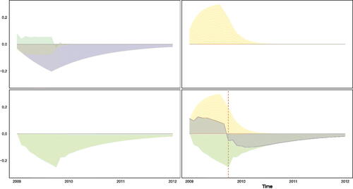
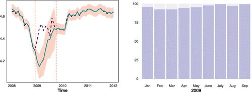
A sneak preview of our results section, given in Figure 1, makes the point: (i) demand-sided effectiveness is shown in the red colored part of its left panel; (ii) intertemporal bias in the form of program reversal is represented by the black part in the left schedule (in particular, seen against the backdrop of the black colored area in the right panel, i.e., a swelling pent-up demand in all other industries, apart from automobiles, after the ending of the subsidy); and (iii) intersectoral bias, even outnumbering effect (i), is highlighted by the red colored area in the right panel of Figure 1.

Figure 1. Distortionary effects of product-specific subsidy on new orders Note: Left panel: automobile sector; right panel: other manufacturing sectors; period: 01/2009 to 06/2012. Red part marks time span of scrappage program: 01/2009 – 09/2009.

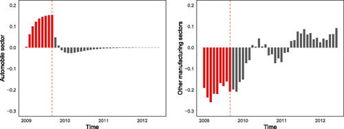
The German 2009 scrappage program, which was in international perspective the most generous one as a share of domestic GDP, amounting to 0.2 percent, is indeed perceived to profoundly have stabilized sales (Haugh et al. 2010). However, we find the demand-side effectiveness of such a temporary product-specific scrappage subsidy to be rather poor. Buyers realize substantial unintended windfall gains that are—as opposed to some alternative schemes one can think of—non-neutral with regard to the public budget. Additionally, stabilization comes, according to our estimates, at the price of a prolongation of the sectoral trough and a retardation of the subsequent recovery in the automobile industry by about one year. This has to be seen against the backdrop of the German automobile sector’s annual turnover amounting to roughly ten percent of German GDP (Schweinfurth 2009). Finally, we are the first to quantitatively document and find evidence for (net) sectoral crowding out and, hence, intersectoral bias of the measure. Thus, our summarizing findings might be seen as speaking in favor of less product-specific alternatives to induce fiscal stimulus, such as consumption vouchers with deadlines, tax incentives, or intervention support in the form of direct government purchases.

Our contribution to the literature and research agenda is to set up and apply an integrated time series approach to systematically and thoroughly disentangle and quantify the different distortions of temporary product-specific subsidies. It is based on Kalman filter estimates of counterfactual time series using information contained in series unaffected from the intervention (in our exemplary application, foreign orders) and on netting out corresponding factual and counterfactual response functions. In doing so, we rely on the identification assumption that domestic and foreign orders are not affected in a substantially different way by an aggregate income shock. This can be rationalized on the grounds of demand for German automotive brands being—due to distinctiveness and lack of international competition—of rather low and equal sensitivity to aggregate shocks (Williamson 2001; Leuwer and Süssmuth 2018).

Since our approach is not firmly based on the well-established potential outcomes model (Rubin 1974, 1978), we need to be careful with the interpretation of our results. We think our approach works well and offers valuable insights regarding the actual effects of crisis and policy on order volumes. Absent a stronger theoretical foundation, however, any causal interpretations are necessarily tentative and, strictly speaking, go beyond our analytical framework.

The remainder is organized as follows. Section 2 briefly rationalizes some theoretical considerations on product-specific subsidization regarding the use of resources and output in the total economy. After some description of our data, we introduce in Section 3 the analytical time series intervention framework to disentangle and quantify the different distortionary effects of temporary product-specific subsidies. In our application, we interpret findings step by step. Section 4 discusses our main findings. Section 5 concludes.

2. Some theoretical considerations

A scrapping bonus is an instrument of fiscal policy that may be used to stabilize an industry in times of economic crisis. To get an idea of the effects of a product-specific scrapping subsidy, we consider a basic theoretical model in the spirit of Harris and Todaro (1970). Detailed underlying equations are given in Appendix A.1. In the following, we focus on a graphical wrap-up as shown in Figure 2.

Figure 2. Transformation curve and change in sectoral output due to subsidy.

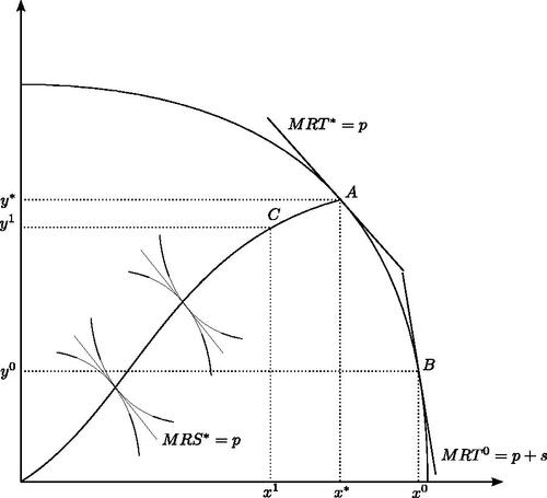
Suppose the total economy initially produces efficiently in point A with output x^* and y^*, where the latter subsumes the output of all other sectors apart from x. Input factors are rewarded their marginal product m in each sector x and remaining industries y. The introduction of a subsidy s for sector x, e.g., a scrapping bonus, will increase the demand for resources and ultimately raise output in sector x at the expense of remaining sectors y. The economy will produce in B (mere substitution effect). Note that a production in B cannot be Pareto-efficient as $MR{S}^{\ast }\ne MR{T}^0$. In case the subsidization of sector x ends, output in sector x (all other sectors y) will decrease (increase).³ Temporarily resources can be unused. Graphically, such a situation is given by point C. For initial resources R₀, production in C would be feasible; however, inputs are not fully employed, i.e., production does not fulfill technical efficiency. Eventually, as m_y decreases the economy will reach a new productively efficient equilibrium with all resources in use. Thus, the challenge is to quantify distance AB and the associated drop in y and increase in x over time of the transitory x-specific subsidy; distance BC, that is the gradual decrease in x at the end and after removal of the subsidy, possibly falling below Pareto-level x^* to x¹; distance CA, that is the recovery to initial levels x^*, y^*. Note that this process—other than shown in Figure 2—might be paralleled by some pent-up demand in y (graphically, this would imply that the concave connecting line between C and A would temporarily even exceed y^*). The final task is to assess the time it takes for re-allocating, that is for the BC, CA re-adjustment.

In the empirical application parts of our study, inefficiency will be measured by estimating a counterfactual scenario without a scrapping bonus. It allows us not only to assess how close to the origin and, hence, off x^* the output in the German automobile sector fell below an efficient level after the ending of the program, but also to assess the price, i.e., the repercussion, of this fiscal stimulus in terms of getting back to an efficient level x^*. In other words, our strategy allows us to measure the true stimulus of the program and the true dip in vehicle sales after the ending of the cash for clunkers program. Additionally, it will provide us with a measure for the actual time of recovery from this dip, i.e. the time elapsed for distance CA in Figure 2. By “true” and “actual” in the last sentences we mean corrected distance and time measures: First, this refers to distance $x^0-x^{\ast }$ corrected for unintentional windfall-profit effects, i.e., considering the volume of vehicles that would have been produced and sold between January and September 2009 anyway without the subsidy. Second, it refers to corrected distance and time elapsed measures for $x^{\ast }-x^1$ taking into account strategic pull-forward effects, i.e., considering consumers having pulled forward their purchases from the future. Naturally, such purchases deepen the cut of sales after the end of a scrappage scheme and delay subsequent recovery. We are aware of the fact that the above argumentation rests on a comparative static model. Nevertheless, we think it will be helpful in structuring and disentangling the effects of the fundamentally dynamic problem of temporary product-specific subsidies.

3. Empirical framework and analysis

The objective of our approach based on counterfactual time series in a kind of event study context is to remove the scrappage program from the observed data but to preserve the equilibrium effects of the recession; see Section 2. It is achieved by relying on three crucial identifying assumptions that are reasonably met for our study:

First, data before the financial crisis is unperturbed by external intervention and can be used to identify the true underlying noise model for each series. This assumption is comparably demanding. However, one can argue that the time from 1991 to 2007 marks a coherent period for the German economy ending with the Great Recession (Dustmann et al. 2014). Moreover, the available pre-crisis time frame of more than one and a half decades can support the assumption of the nullification of previous interventions.

Second, there is no substantial change contemporaneous with the program. It is justified as the German scrappage scheme was sector-specific and internationally exceptional in size as well as anticipatory in timing.

Third, the association of foreign with domestic orders is stable and persisted during the crisis. It is justified as demand for German cars is, due to distinctiveness and lack of international competition, in domestic and foreign markets of rather low and uniform sensitivity to aggregate income shocks (Williamson 2001).

Our methodological approach is based on intervention analysis by Box and Tiao (1975). In its aim to assess the effects of a known intervention, it is related to the potential outcomes framework—the so-called Rubin Causal Model (Holland 1986; Rubin 1974)—and accompanying econometric methods (Imbens and Rubin 2015). Nonetheless, there is a gap between both methodologies as intervention analysis decidedly focuses on a time series setting. It utilizes the information from one single time series directly. The majority of methods based on the Rubin Causal Model do not involve the use of ARIMA models which are predominant in modern time series analysis. Both difference in differences (DiD) estimators (Roth et al. 2023) and synthetic controls (Abadie et al. 2010) are not well suited when dealing with a long pre-treatment period. They are not designed to capture and use the dynamic information within a time series. On the other hand, these methods are firmly based on the potential outcome framework which is generally not the case for intervention analysis. However, unless such a theoretical foundation is established and the effect under consideration is clearly defined, intervention analysis suffers from an attribution problem. The estimated coefficients are not analytically attributable to the intervention in a precise manner and a causal interpretation of the estimated effect may not be warranted (Menchetti et al. 2021, 2022).⁴

Another time series-based method to evaluate the effects of an exogenous intervention is interrupted time series (ITS) analysis (Lopez Bernal et al. 2016). This method assumes that the evolution of a time series can be modeled with a deterministic trend in linear regression models and compares resulting trend fits before and after an intervention. The method is also not based on ARIMA models.⁵ Since our time series follow a stochastic trend and since we are interested in using long-run information on the underlying dynamic structure of the data generating process (DGP), ITS seems not appropriate for our analysis.

The following analysis is fully implemented in R. The packages used for estimation are forecast by Hyndman and Khandakar (2008), TSA by Cryer and Chan (2009), and astsa by Shumway and Stoffer (2011). Our approach on netting out factual and counterfactual response functions for domestic and foreign new orders is based on the missing value imputation procedure described in Shumway and Stoffer (2011). The descriptive statistics and Jarque-Bera tests in Table 3 have been computed with the moments package by Komsta and Novomestky (2022).

3.1. Sectoral time series

We consider seasonally adjusted monthly data from January 1991 to June 2012 on order book levels in twelve industries of the German manufacturing sector.⁶ The data is supplied as volume index by the German Statistical Office. The industries considered are electronical and optical devices, clothing, chemicals, electronics, cars, metalworking, production of paper, pharmaceutics, textiles, machines, production of metal, and vehicles other than cars. Figure 3 shows the data for the twelve considered industries separated by orders from foreign markets (green) and from inland (violet).

Figure 3. Log order book levels with foreign (green) and inland (violet) origin Note: Period: 01/1991 to 06/2012. Three vertical grey lines mark 08/2007 (beginning of the financial crisis), 09/2008 (collapse of Lehman Brothers), and 10/2009 (onset sovereign debt crisis in euro area). Red crosses indicate local turning points. Two-digit NACE ‘08 codes in parenthesis. For descriptive statistics and official descriptions see Appendix A.2.

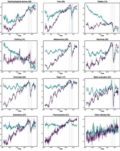
The three vertical grey lines mark the beginning of the financial crisis on August 9, 2007 (hallmarking the start of rapid increase of the interbank interest rate in the US),⁷ the collapse of Lehman Brothers in September 2008, and the beginning of the sovereign debt crisis in the euro area in October 2009, respectively. The blue shaded area in the upper panel in the middle column identifies the scrapping bonus in the automobile industry that was in place from January 2009 to September 2009. In each panel the two red crosses mark lower turning points, i.e., the minimum of orders between the first and third vertical line, respectively.

As can be seen from Figure 3, the crisis effect varies by sector. There seem to be three stylized types of reaction: industries that are seemingly unaffected by the crisis (e.g., vehicles other than cars), industries that were affected by the crisis but recovered quite fast (e.g., electronics), and industries in which orders shifted downwards and did not recover up to the end of our observation period (e.g., clothing).

The German automobile industry is the only one of the sectors shown in Figure 3 that could directly benefit from policy measures undertaken to dampen the crisis’ impact. Although the bonus was officially introduced to increase the fuel efficiency of the German households’ vehicle stock, there is no doubt it was intended as fiscal stimulus. Table A.1 in the Appendix provides wider descriptions and summary statistics of the series underlying Figure 3.

3.2. Intervention analysis

Intervention analysis, dating back to the seminal contribution by Box and Tiao (1975), is a straightforward technique to back up our approach and assess the effect of an intervention on a time series. This holds in particular with regard to potential changes of its first moment. Consider a time series {y_t} that may be modeled by some ARIMA($p,d,q$) process. An intervention model then is written as (3.1) $$\begin{array}{l}{y}_t=\nu (L)I_t+\frac{{\mathrm{\Theta }}_q(L)}{{\mathrm{\Phi }}_p(L)}{z}_t=m_t+n_t.\end{array}$$(3.1)

In (3.1(3.1) $$\begin{array}{l}{y}_t=\nu (L)I_t+\frac{{\mathrm{\Theta }}_q(L)}{{\mathrm{\Phi }}_p(L)}{z}_t=m_t+n_t.\end{array}$$(3.1) ) n_t is the noise model and m_t represents the change in the mean function due to an intervention. The lag polynomial ν(L) determines the shape and the duration of the series’ reaction to a shock. ν(L) is approximated by the following rational function (3.2) $$\begin{array}{l}\nu (L)=\frac{\omega (L)}{\delta (L)}{L}^a,\end{array}$$(3.2) where the exponent a∈ℕ₀ determines the amount of time that passes before y_t reacts to an intervention; and ω(L) and δ(L) are polynomials in L of order s and r, i.e., $\omega (L)={\omega }_0+{\omega }_{1}L+...+{\omega }_s{L}^s$ and $\delta (L)=1-{\delta }_{1}L-...-{\delta }_r{L}^r$. The coefficients ω_j in the numerator of (3.2(3.2) $$\begin{array}{l}\nu (L)=\frac{\omega (L)}{\delta (L)}{L}^a,\end{array}$$(3.2) ) capture the immediate effect of an intervention while the coefficients δ_r of the denominator model the permanent effect of the intervention.

Coefficients ν_j of ν(L) are calculated from δ(L)ν(L) = ω(L)L^a, that is $$\begin{array}{ll}& (1-{\delta }_{1}L-...-{\delta }_r{L}^r)({\nu }_0+{\nu }_{1}L+{\nu }_2{L}^2+...)\\ & =({\omega }_0+{\omega }_{1}L+...+{\omega }_s{L}^s)L^a.\end{array}$$

This implies that $$\begin{array}{l}{\nu }_j=\{\begin{array}{l}0\text{ for }j<d\\ {\delta }_1{\nu }_{j-1}+{\delta }_2{\nu }_{j-2}+...+{\delta }_r{\nu }_{j-r}+{\omega }_{j-d}\\ \text{ for }j=d,d+1,..,d+s\\ {\delta }_1{\nu }_{j-1}+{\delta }_2{\nu }_{j-2}+...+{\delta }_r{\nu }_{j-r}\text{ for }j>d+s.\end{array}\end{array}$$

In general, we can think of three different stylized types of intervention responses:

1. Impulse function (IF) (3.3) $$\begin{array}{l}{I}_t:={ϵ}_t^{(\tau )}=\{\begin{array}{l}1\text{ for }t=\tau \\ 0\text{ for }t\ne \tau ,\end{array}\end{array}$$(3.3)

2. Extended impulse function (EIF) (3.4) $$\begin{array}{l}{I}_t:={\eta }_t^{({\tau }_1,{\tau }_2)}=\{\begin{array}{l}1\text{ for }{\tau }_1\le t\le {\tau }_2\\ 0\text{ for }t\text{ else},\end{array}\end{array}$$(3.4)

3. Step function (SF) (3.5) $$\begin{array}{l}{I}_t:={\zeta }_t^{(\tau )}=\{\begin{array}{l}1\text{ for }t\ge \tau \\ 0\text{ for }t<\tau .\end{array}\end{array}$$(3.5)

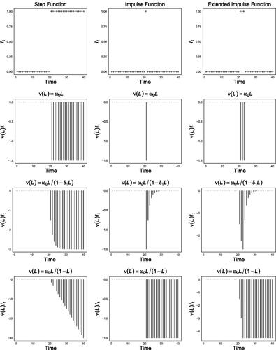
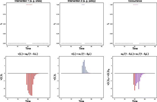
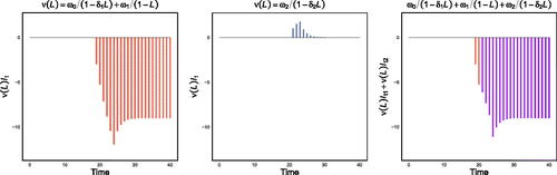
Figure 4 showcases the shape of m_t for different intervention response types along its column dimension: SF: $I_t:={\zeta }_t^{(\tau )}$ in its first column, IF: $I_t:={ϵ}_t^{(\tau )}$ in its second column, and EIF: $I_t:={\eta }_t^{({\tau }_1,{\tau }_2)}$ in its third column, respectively. Transfer function specifications are displayed along the row dimension: ν(L) = ω₀L^a with a = 0 and ${\omega }_0=(-1.5)$ in the second row, $\nu (L)={\omega }_0/(1-{\delta }_{1}L)L^a$ with a = 0, ${\omega }_0=(-1.5)$ and δ₁ = 0. 5 in the third row, $\nu (L)={\omega }_0/(1-{\delta }_{1}L)L^a$ with a = 0, ${\omega }_0=(-1.5)$ and δ₁ = 1. 0 in the fourth row, respectively.

Figure 4. Mean reaction to different intervention types and transfer functions Note: First column: $I_t:={\zeta }_t^{(\tau )}$, second column: $I_t:={ϵ}_t^{(\tau )}$, third column: $I_t:={\eta }_t^{({\tau }_1,{\tau }_2)}$. Second row: ν(L) = ω₀L^a with a = 0 and ${\omega }_0=(-1.5)$, third row: $\nu (L)={\omega }_0/(1-{\delta }_{1}L)L^a$ with a = 0, ${\omega }_0=(-1.5)$ and δ₁ = 0. 5, fourth row: $\nu (L)={\omega }_0/(1-{\delta }_{1}L)L^a$ with a = 0, ${\omega }_0=(-1.5)$ and δ₁ = 1. 0.

The Box-Tiao approach can account for multiple interventions. This feature differentiates it from more common approaches like synthetic controls or DiD which are designed to evaluate unique interventions. In our case, we have a concurrence of two separate interventions: crisis and scrappage program. Therefore, intervention analysis seems well-suited.

To additionally account for the policy, we add a second extended impulse function ${\eta }_{t,2}^{({\tau }_3,{\tau }_4)}$ with ${\tau }_3=01/2009$, ${\tau }_4=09/2009$. Due to the temporary nature of the program, we exclude a step function and assume a simple specification of low order for all sectors considered. Specifically, (3.6) $$\begin{array}{l}{m}_t^P=\frac{{\omega }_0^P}{1-{\delta }_1^{P}L}{\eta }_{t,2}^{({\tau }_3,{\tau }_4)}\end{array}$$(3.6)

A fully specified multiple intervention model that accounts for both the crisis and the policy has the general functional form (3.7) $$\begin{array}{l}{y}_t=m_t^C+m_t^P+n_t\end{array}$$(3.7) where superscript P denotes the mean function due to policy intervention and superscript C the mean function due to crisis intervention.

Figure 5 schematically shows the underlying idea. Although observing one single time series only, by specifying the functional forms of the effects of individual interventions (first and second column-panel), the method allows for disentangling the combined effect shown in the third column-panel of Figure 5.

Figure 5. Stylized transfer functions for crisis effect and scrapping bonus effect Note: The following parameter values are assumed: ${\omega }_0=(-1.5)$, δ₁ = 0. 5, ω₁ = 1. 0 and δ₂ = 0. 5.

The fitting of intervention models is an iterative and tentative process (Box and Tiao 1975; Hibbs 1974). It blends extra-econometric knowledge, structural form assumptions about the intervention as well as interpretations of the observed data in choosing an appropriate econometric specification. Specifically, we proceed along the following lines:⁸

1. Find an ARIMA($p,d,q$)-process of appropriate order for the noise model n_t based on the pre-intervention data. Determining the model order is done by minimizing the Akaike information criterion (AIC) over a sensible range of possible values for p and q. The order of integration is fixed for all our series, i.e., d = 1. Confirming with the Ljung-Box test that pre-intervention residuals are white noise completes this step.

2. Initially focus on the crisis impact: select the intervention type by visually inspecting the time series and assessing the permanent (suggesting a SF) or temporary (EIF) nature of the change during the intervention.

3. Choose functional form of transfer function for crisis impact via minimization of the AIC augmented with likelihood-ratio tests of significance. If AIC selects zero or two lags for δ(L), test model against model with one lag. Select latter specification if not significantly different from AIC-selected competitor (5% level).

4. Augment model derived in previous step: allow for second intervention (policy). Assume an extended impulse and a simple transfer function with r = 1 and s = 0 for δ(L) and ω(L), respectively.

5. Keep augmented model if AIC is lower than before and if augmented model is—at least at the 10 percent significance level—statistically different from reduced model without the policy.

6. Testing the white noise assumption of model residuals on the full available time span with the Ljung-Box test completes the procedure.

Step 5 ensures selection of models where the mean specification m_t is credible and statistically significant. Step 3 mirrors our preference for dynamically informative yet simple specifications. It acts as a safeguard against overfitting.

In the following, we estimate intervention models for foreign and domestic orders as described above and interpret the direct model outcomes.

Subsequently, we make use of the information contained in foreign orders series that were unaffected by the domestic scrappage scheme⁹ to estimate counterfactual intervention-free reactions sector by sector. This strategy allows us to assess intertemporal strategic pull-forward effects and separate them from unintentional windfall profits and intersectoral distortions.

3.3. Fitting intervention models to economic sectors

The choice of a noise model n_t is based on pre-intervention data ranging from 01/1991 to 07/2007. We exclude the time after 07/2007 as the beginning of the financial crisis is an intervention that potentially impedes the identification of the correct underlying noise model. Although a relevant intervention prior to our horizon of interest, we do not need to account for this crisis in our model. By basing the underlying noise model on—as is assumed—normal times, we capture the usual dynamics of the time series and can use this information during non-normal times. Every earlier intervention not included in our model is captured by the residuals. As long as these interventions are uncorrelated, the estimates should still be consistent. We formally check this assumption post model selection and estimation.

Appropriate AR and MA orders are found by minimizing the AIC over a reasonable range of values for p and q. All series are assumed to be integrated of order one, i.e. d = 1. An overview of the suggested noise model using the AIC, Bayesian information criterion (BIC), and corrected AIC (the AICC) is given in Table A.2 in Appendix A.3. The proposed specifications are identical in most cases. If different, the AIC tends to select longer lags and the Ljung-Box test statistic is on average higher. Yet, results are relatively stable with regard to the information criterion used.¹⁰

When setting up $m_t=m_t^C+m_t^P$, we begin by focusing on the crisis intervention captured by $m_t^C$. First, we choose the respective intervention type. In most cases, the crisis impact is modeled as an EIF ${\eta }_t^{({\tau }_1,{\tau }_2)}$ with τ₁ = 09/2008 and τ₂ = 10/2009. This seems to be a reasonable choice with regard to the course of the crisis and the general shape of the series under study. However, one might argue that the financial crisis directly carried over into the European sovereign debt crisis. In this case, the crisis impact could also be modeled as a step function ζ^τ with τ = 09/2008. Given our series at stake, this seems to be the more appropriate strategy in the case of the clothing (domestic and foreign) and pharmaceutical industries (domestic) as well as the textiles industry (foreign).¹¹ See Figure 3 for a visual impression of crisis impacts.

For most industries, we observe quite an instantaneous drop in log new orders after 09/2008. Hence, setting a = 0 in Equation (3.2) seems justified for the majority of cases. Only for the clothing industry, the series’ reaction to the collapse of Lehman Brothers is slightly delayed by about three months. Thus, we set a = 3 for this sector.

As regards the shape of the transfer function ν(L), fairly parsimonious specifications, like the ones shown in the third row of Figure 4, prove adequate. In some cases, a higher order of the polynomial δ(L) is suggested by the AIC. After comparing these models to a polynomial of order one with the likelihood-ratio test, we keep a second-order polynomial for electronics (domestic and foreign), production of paper (domestic), textiles (domestic), production of metal (domestic), and vehicles other than cars (foreign). For new domestic orders of electronical and optical devices, the AIC selects a polynomial of degree zero. When testing against a higher-order polynomial of order one, we cannot reject the null hypothesis that both models are equivalent and choose the latter more informative specification. Only in the case of foreign new orders in pharmaceutics, we keep the most simple specification due to modeling restrictions. A detailed overview of AIC-suggested models and our deliberate deviation from these suggestions in three cases is given in Table A.3 in Appendix A.4.

After fixing the mean specification for the crisis, we allow for the inclusion of the scrappage program as described in Section 3.2. Note, however, that we allow an effect of the policy on domestic demand only. Foreign orders are presumed to be unaffected by the domestic scrappage scheme. This assumption is plausible, as only German citizens were entitled to apply for the premium.

Both intervention type and transfer function for $m_t^P$ are fixed. We test the additional coefficients for joint significance and keep the restricted model without the policy in case the policy effect is not significantly different from zero, at least, at the 10 percent level. Only in case of clothing (p = 0. 001), electronics (p = 0. 018), automotive (p = 0. 000), pharmaceuticals (p = 0. 068), and the metal producing (p = 0. 081) sectors, we can reject the null hypothesis and keep the policy in the mean function.¹²

Table A.4 in the Appendix gives an overview of intervention models fitted to the log series. The last two columns of the table show the exact transfer functions. Table A.5 complements this overview. It gives for all models their estimated coefficients and standard errors with corresponding AIC and Ljung-Box test statistic based on 20 lags. The hypothesis that there is no significant residual correlation left cannot be rejected in most cases.¹³

3.4. Analyzing the non-subsidized sectors

We begin by analyzing the effect of the crisis on the non-subsidized sectors and control for the effect of the scrappage program if appropriate. A discussion of the effects of the policy is reserved for later sections. Here we focus on the estimated total effect in sectors not directly targeted by the policy.

Figure 6 plots the time series along with fitted values and respective estimated stylized crisis effect. Table 1 reports the estimated percentage decrease in vehicle orders due to the crisis k months after 09/2008 for different industries.

Table 1. Crisis effect as percentage drop in orders k months after 09/2008.

Sector	Order Origin	k										$t{|}_{m_t=0}$
			1	2	3	6	9	12	15	18	21	24
26	Inland	−3.82	−0.58	−3.33	−1.30	−2.53	−1.78	1.58	−0.96	0.59	−0.36	19
	Foreign	−4.04	−7.25	−9.79	−14.67	−17.10	−18.31	−14.86	−7.40	−3.69	−1.84	27
14	Inland	0.00	0.00	0.00	−18.11	−21.55	−22.20	−22.33	−22.35	−22.35	−22.35	∞
	Foreign	0.00	0.00	0.00	−44.39	−44.39	−44.39	−44.39	−44.39	−44.39	−44.39	∞
20	Inland	−3.99	−7.09	−9.52	−14.03	−16.17	−17.18	−13.68	−6.48	−3.07	−1.46	26
	Foreign	−3.22	−8.68	−15.03	−26.57	−18.20	−7.31	−7.60	0.89	5.98	0.88	28
27	Inland	−3.80	−10.35	−18.10	−38.60	−34.98	−25.49	−24.83	−13.29	−4.07	−6.38	33
	Foreign	−7.42	−9.44	−14.11	−21.99	−28.15	−32.43	−28.11	−21.21	−14.90	−10.72	∞
29	Inland	See section 3.4
	Foreign
25	Inland	−5.13	−9.34	−12.79	−19.83	−23.71	−25.84	−21.88	−12.05	−6.63	−3.65	31
	Foreign	−6.78	−12.30	−16.79	−25.88	−30.80	−33.46	−28.12	−15.21	−8.23	−4.45	32
17	Inland	−1.23	−3.35	−5.89	−11.36	−9.42	−4.55	−2.62	1.20	2.45	0.19	14
	Foreign	−3.12	−5.50	−7.31	−10.54	−11.96	−12.59	−9.75	−4.31	−1.91	−0.84	23
21	Inland	−2.49	−4.79	−6.90	−18.47	−24.06	−27.43	−23.76	−24.32	−25.72	−26.90	∞
	Foreign	-	-	-	-	-	-	-	-	-	-	-
13	Inland	−6.58	−6.41	−11.08	−13.91	−17.70	−18.50	−13.24	−9.19	−4.22	−3.05	30
	Foreign	−4.34	−10.70	−17.20	−27.91	−25.95	−22.38	−21.97	−22.87	−23.23	−23.07	∞
28	Inland	−7.52	−14.07	−19.80	−32.96	−41.71	−47.53	−43.88	−29.17	−19.40	−12.90	∞
	Foreign	−5.53	−12.97	−20.34	−35.41	−40.76	−41.79	−36.19	−14.88	−3.50	−0.12	21
24	Inland	−5.41	−15.04	−26.92	−48.93	−33.21	−2.95	−1.95	1.03	3.62	0.40	14
	Foreign	−8.33	−14.31	−18.59	−25.46	−27.99	−28.93	−20.95	−7.73	−2.86	−1.05	24
30	Inland	-	-	-	-	-	-	-	-	-	-	-
	Foreign	−10.66	−19.88	−27.86	−45.92	−57.61	−65.19	−59.44	−38.51	−24.95	−16.16	∞

Note: Models based on AIC. The last column indicates after how many months the effect has vanished (= 0).

Figure 6. Log series, fitted values and implied sectoral stylized reactions (crisis effect) Note: Solid line shows logarithm of raw data, red dotted line fitted values. Grey vertical lines mark 08/2007, 09/2008, and 10/2009. Results for the German automobile industry are shown separately in Section 3.5. Industry 12 vehicles other than cars is not shown due to being not significantly affected by the crisis.

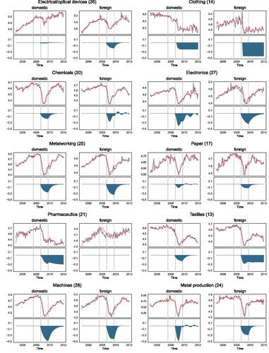
Some results stand out. First, in general, orders from abroad seem to have been affected by the crisis more severely than domestic orders. This result fits common wisdom as economies coined by strong exporting industries are generally considered to be most severely hit by an international crisis. One obvious exception is the pharmaceutical industry. Offshore orders in this particular industry seem not to have been affected post-Lehmann, whereas domestic orders decreased significantly and kept on fluctuating around a lower level than before the crisis.¹⁴ But also in the electronics, machinery, and production of metal industries foreign orders are slightly less affected by the crisis. Across industries, however, the decrease in foreign orders on average was approximately 4% higher than the one in domestic orders.

Second, concerning the absolute size of the crisis impact, the German machinery, clothing, and vehicles other than cars industries were most seriously hit; see Figure A.10 in Appendix A.12. Twelve months after the collapse of Lehman Brothers domestic (foreign) orders in the machines sector had decreased by around 47% (42%); domestic orders in the vehicles other than cars industry by 65%. Foreign orders in the clothing sector have been reduced heavily by almost 45%. This is twice the reduction in domestic orders. Finally, we find industries that did not recover up to mid-2012. These are the clothing industry (domestic and foreign), as well as foreign orders in the electronics, textiles, and vehicles other than cars industries. For domestic orders, pharmaceutics and the machinery industry show a persistent decline in order volumes after the crisis. This persistency is also indicated by $t{|}_{m_t=0}=\mathrm{\infty }$ in the last column of Table 1.

3.5. Analyzing the subsidized sector

We now turn to the automotive sector explicitly targeted by the domestic scrappage program. Precise coefficient estimates are shown in Appendix A.6. The exact transfer function is given in Appendix A.5. All estimated coefficients are highly statistically significant for both domestic and foreign orders. The Ljung-Box test rejects the null of serial correlation in the residuals for both series. For domestic orders, the likelihood-ratio test supports the inclusion of the policy with a p-value near zero. When including the policy, the crisis effect is captured by ${\omega }_0^C$ and ${\delta }_1^C$ which are expected to be negative and positive, respectively. The effect of the policy is captured by ${\omega }_0^P$ and ${\delta }_1^P$. Both are expected positive. Estimates are fully in line with these priors.

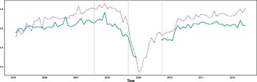
Estimation results are shown in Figure 7 and Table 2. The right column of diagrams in Figure 7 shows the log of foreign vehicle orders together with fitted values (upper panel) and the estimated crisis effect (lower panel). The left panel shows the same for domestic orders. Table 2 is the complement to Table 1. It shows the estimated impact of crisis and policy on domestic orders as well as the pure crisis effect on foreign orders in the automobile sector.

Table 2. Crisis effect as percentage drop in orders k months after 09/2008. Note: Models based on AIC. The last column indicates after how many months the effect has vanished (= 0).

Sector	Order Origin	k										$t{|}_{m_t=0}$
			1	2	3	6	9	12	15	18	21	24
29	Inland	−8.45	−14.98	−20.03	−11.62	−6.47	−5.84	−15.24	−9.40	−4.99	−2.49	28
	Foreign	−4.49	−12.39	−21.96	−41.25	−27.73	−5.56	−5.93	−1.15	5.02	2.74	22

Figure 7. Series, fitted values and estimated crisis effect and scrapping bonus effect.

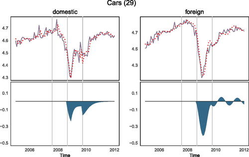
Table 2 shows the automobile industry’s reaction to the crisis. Compared to the crisis effect estimates of other industries in Table 1, the automobile sector’s reaction is not idiosyncratic. This concerns both the size of the negative effect and the fact that foreign orders were hit more severely than domestic orders. However, when comparing the stylized dips for foreign and domestic orders, the latter seem negatively affected for a longer period than foreign orders. Moreover, the implied effect for domestic orders is unique in its double-dip appearance. It points to the effects of the scrappage program that will be analyzed in more detail in the next section. In sum, we see a strong indication that the temporary product-specific subsidy has led to structural disruptions. These substantially prolong both impact and aftermath of the crisis through pull-forward effects of car sales.

Before proceeding with the disentanglement of estimated crisis and policy effects, let us consider in how far our modeling assumptions are fulfilled. Specifically, we need to check if the residuals are approximately white noise as this is the central assumption of intervention analysis à la Box and Tiao (1975). Ideally, the residuals are Gaussian white noise. However, since we assume that our underlying noise model captures the true data-generating process and that all potential interventions apart from the ones we are interested in are absorbed by the residuals, we should not expect normally distributed residuals.

Table 3 displays the corresponding robustness checks for the residuals from our estimated intervention models. It shows skewness, kurtosis, the Jarque-Bera normality test, and the Ljung-Box test for white noise. We have to reject the central assumption of white noise residuals only in two cases for domestic orders—electronics (27) and metal production (24)—and in two cases for foreign orders—textiles (13) and metal production (24). However, and as expected, in the majority of cases the Jarque-Bera null hypothesis of normality is rejected.

Table 3. Robustness checks for AIC-selected intervention models.

		Sector
		26	14	20	27	29	25	17	21	13	28	24	30
Skewness	inland	0.10	0.08	−0.66	0.77	−0.50	−0.08	0.31	−0.46	0.14	−0.11	0.15	1.49
	foreign	−0.22	0.14	0.08	0.38	0.71	0.67	−0.21	0.43	0.43	0.14	0.27	0.12
Kurtosis	inland	5.19	3.44	4.71	6.86	5.19	3.74	3.93	6.56	2.85	3.14	4.94	6.44
	foreign	3.85	6.62	3.07	3.54	7.50	4.94	3.33	4.34	4.07	3.51	4.40	2.49
Jarque-Bera	inland	0.00	0.31	0.00	0.00	0.00	0.05	0.00	0.00	0.59	0.70	0.00	0.00
	foreign	0.01	0.00	0.85	0.01	0.00	0.00	0.22	0.00	0.00	0.16	0.00	0.18
Ljung-Box	inland	0.82	0.47	0.50	0.00	0.72	0.16	0.82	0.71	0.82	0.70	0.04	0.19
	foreign	0.46	0.94	0.19	0.66	0.96	0.87	0.26	0.39	0.05	0.79	0.02	0.56

As the Jarque-Bera test is based on skewness and kurtosis, the specific constellation leading to a rejection of the null is informative in the present context. Table 3 shows that overall, the residuals—except for the other-vehicles-sector (30)—exhibit only a mild skewness. The kurtosis, however, deviates considerably from the theoretical value of three in the majority of cases where we have to reject the null of normality. This is exactly what is expected if interventions occur more frequently than implied by a normal distribution. That is, one would expect a leptokurtic distribution. Being unsystematic, multiple interventions should also balance out regarding their effective direction. If these interventions do not systematically change the way the underlying system behaves, the effects of such interventions should die out. This is what is seen when acknowledging the serially uncorrelated and symmetrically distributed residuals.

In consequence, we can still assume that our central modeling assumptions are fulfilled. Although not normally distributed, the residuals generally are symmetrically distributed and serially uncorrelated. Our models capture the general dynamics of the underlying time series without having to include additional intervention terms due to the residuals statistically behaving like independently distributed white noise. Hence, the majority of point estimates from our intervention models should be consistent.¹⁵

3.6. Disentangling by using implied filters

Given our estimates of the effects of crisis and, if appropriate, policy, we can now disentangle the individual interventions’ contributions. As discussed in Section 3.3, specifications for clothing, electronics, automotive, pharmaceuticals, and the metal producing sectors include a mean function to capture the effects of the scrappage program. However, despite being statistically significant, we exclude the clothing sector in the following analysis due to economically implausible results and negligible quantitative impact.¹⁶

Figure 8 shows the individual contributions to the total crisis and policy effect for each relevant sector. The blue area in the upper part of each quadrant marks the policy, and the red one the crisis effect. The violet area in the corresponding lower schedule shows the combined effect. This is juxtaposed with an estimate from a reduced model that lacks the policy function, shown in grey.

Figure 8. Constituents of total effect of crisis and policy. Note: Upper panel in each quadrant shows crisis effect (red) and policy effect (blue). Each quadrants lower panel shows total effect (violet) in contrast to total effect from pure crisis model without policy (grey). Shown are sectors with significant effect of scrappage program. Grey vertical lines mark 08/2007, 09/2008, and 10/2009.

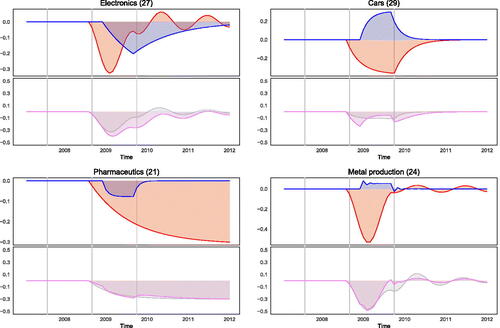
In all cases, the inclusion of the policy is relevant and alters the shape of the estimated crisis effect. For the automotive sector, the estimates confirm both a moderating and prolonging effect of the policy. The finding for the connected metal producing sector is sensible and indicates a policy-induced shortening of the crisis. In case of electronics, the policy indicates a sizeable negative effect significantly deepening and prolonging the crisis in this sector. Only in case of pharmaceutics, the overall effect is roughly the same and the policy seems to have no long-run effects of either prolonging or shortening nature.

Summing up the policy effects from the other affected sectors and comparing them to the automotive sector gives Figure 9. Our estimates support the hypothesis of intersectoral distortions. The effect on the automobile sector (upper right panel, yellow) is estimated positive throughout. The total effect on other affected sectors is negative (lower left panel, green). Their difference is positive during the program and turns negative thereafter (lower right panel). These estimates do not show indications of pent-up demand. Instead, they support the idea of a negative net effect from the policy with enduring cuts on demand over the time horizon considered.¹⁷

Figure 9. Comparing policy effect in subsidized and non-subsidized sectors Note: Upper left panel shows other sector’s individual policy reactions. Upper right panel shows automobile sector’s policy reaction. Lower left panel shows total of other sector’s effects. Lower right panel shows total effect in automobile sector (yellow), other sectors (green) and as net effect their difference (grey). Dashed red line marks end of scrappage program.

These results have to be taken with a pinch of salt. Not all findings are robust with regard to the underlying noise model; see Appendix A.9. Especially the spillover effects on other sectors are sometimes volatile in size and direction. The result for the automotive sector, however, is robust. This seems reasonable as the effect in the automobile sector counteracts the crisis by design. In other sectors we might even expect converging effects. Given the scrappage policy explicitly targets it, we can expect a large effect relative to the crisis in the automobile sector. Potential spillover effects, however, spread over multiple sectors and can be expected to be relatively low when compared to the overall crisis effect. Given we identify crisis and policy with binary indicators which differ only for 5 out of 14 months, the estimation procedure is expected to experience difficulties. We, thus, augment and complement our procedure in the next section.

3.7. Disentangling by estimating counterfactual intervention-free reactions

3.8. Strategic pull-forward effect

The German scrapping bonus, just like the cash for clunkers program (officially named “Car allowance rebate system” or briefly CARS; see Goolsbee and Krueger 2015) in the United States that the US federal government started coinciding with the phase-out of the German program, induced sales of additional cars in the short run. However, it might have led to a substantial reversal in the sense of households “front-loading” their expenditures for vehicles in the medium run (Mian and Sufi 2012). It is straightforward to suppose that consumers who had planned to buy a new car in 2010 or later anyway pulled forward their purchases of new vehicles due to the subsidy.¹⁸ This in turn could have led to a situation in which vehicle orders and purchases did not normalize after the end of the scrapping bonus or of the crisis. We may test this by using a model specification that differs from the one used hitherto. The idea is to test two different specifications for m_t against each other. The first one just as the preceding ones assumes that vehicle orders got back on track after the subsidy and/or the crisis had ended. That is, that there was no permanent shift in the mean of the series. The second possible specification presumes that orders remained on a new lower level after 2009. In this case, the mean equation for the policy $m_t^P$ has the following form (3.8) $$\begin{array}{l}[\frac{{\omega }_0}{1-{\delta }_{1}L}+\frac{{\omega }_1}{1-{\delta }_{1a}L}]{\eta }_{t,1}^{({\tau }_1,{\tau }_2)}\end{array}$$(3.8) where δ_1a = 1.

The estimated effect will then represent stylized reactions as shown in Figure 10.

Figure 10. Stylized transfer function specification for a permanent drop in vehicle orders. Note: The following parameter values are assumed: ${\omega }_0=(-1.5)$, δ₁ = 0. 5, ${\omega }_1=(-1.5)$, ω₂ = 1. 0 and δ₂ = 0. 5.

When modifying the specification of the transfer function according to (3.8(3.8) $$\begin{array}{l}[\frac{{\omega }_0}{1-{\delta }_{1}L}+\frac{{\omega }_1}{1-{\delta }_{1a}L}]{\eta }_{t,1}^{({\tau }_1,{\tau }_2)}\end{array}$$(3.8) ) the resulting estimate for ω₁ is of expected sign though not statistically significant. The AIC value of the new model increases to −864. 28. The results are economically implausible by implying a huge negative effect of the policy that would dwarf the crisis; see Figure A.11 in Appendix A.12. Thus, we conclude that the more parsimonious model is justified.

In line with our intuition, there seems to be no evidence that pull-forward sales by implying structural disruptions in the automobile market have led to a permanent decrease in vehicle orders following the crisis and/or the scrappage program. Nevertheless, “front-loading” of household expenditures on vehicles most probably prevented the German automobile industry from recovering as fast as would have been possible.¹⁹ As initially suspected, it led to a transitory decrease in vehicle orders following the end of the scrapping bonus; see Table 2. In what follows, we compute and visualize this externality by estimating the net effect of the scrappage scheme.

3.9. Unintentional windfall-profit effect

In the following, we seek to calculate the hypothetical crisis effect in the absence of a scrapping subsidy to quantify a potential and frequently debated free-rider effect of such bonus measures. The idea is to address the question of how many cars would have been ordered between January and September 2009 if there had been no subsidizing program. Thus, the aim is to assess the ineffective part of the scrappage scheme by also accounting for the fact that vehicle orders might have regained over the year after January 2009 even without the installation of the program.²⁰

This quantitative assessment is done in three steps. First, we assume that the series for domestic vehicle orders was not observed between January and September 2009; see Figure 11. Second, we transform the series for foreign and domestic orders, where the latter is only partially observed, into a state-space representation and estimate values for the missing observations by applying the Kalman filter.²¹ Based on the filtered values for the missing observations, we then can calculate what the crisis impact on the German automobile industry would have been without the scrapping subsidy, i.e., the net effect.²²

Figure 11. Log orders, missing observations 01/09 to 09/09 for inland orders (dashed).

A particular advantage of state-space modeling is its ability to treat time series with missing observations (Stoffer 1982; Jones 1980). Shumway and Stoffer (2008) describe the necessary modifications to fit multivariate state-space models to data with missing observations. The exact state-space model used in the present context, based on Equations (A.13.1(A.13.1) $$\begin{array}{l}{\mathit{y}}_t={\mathit{Z}}_t{\mathit{\alpha }}_t+{\mathit{d}}_t+{\mathit{u}}_t,t=1,...,T.\end{array}$$(A.13.1) ) and (A.13.2(A.13.2) $$\begin{array}{l}{\mathit{\alpha }}_t={\mathit{T}}_t{\mathit{\alpha }}_{t-1}+{\mathit{c}}_t+{\mathit{R}}_t{\mathit{\nu }}_t,t=1,...,T.\end{array}$$(A.13.2) ) in Appendix A.13.1, is given by $$\begin{array}{ll}{\mathit{Z}}_{\mathit{t}}& ={\mathit{R}}_{\mathit{t}}=\left(\begin{array}{cc}1& 0\\ 0& 1\end{array}\right),{\mathit{T}}_{\mathit{t}}=\left(\begin{array}{cc}{\varphi }_{11}& {\varphi }_{12}\\ {\varphi }_{21}& {\varphi }_{22}\end{array}\right),{\mathit{c}}_{\mathit{t}}={\mathit{d}}_{\mathit{t}}=\left(\begin{array}{c}0\\ 0\end{array}\right),\\ {\mathit{H}}_{\mathit{t}}& =\left(\begin{array}{cc}{\sigma }_1^2& {\sigma }_{12}\\ {\sigma }_{12}& {\sigma }_2^2\end{array}\right),{\mathit{Q}}_{\mathit{t}}=\left(\begin{array}{cc}{\sigma }_3^2& {\sigma }_{34}\\ {\sigma }_{34}& {\sigma }_4^2\end{array}\right).\end{array}$$

The corresponding observational vector 𝐲_𝐭 contains foreign and domestic orders for each sector.

Parameters are derived via ML estimation using the expectation maximization (EM) algorithm by Shumway and Stoffer (2011). Missing values are handled as described below.

The general starting point is again a model as given by Equations (A.13.1(A.13.1) $$\begin{array}{l}{\mathit{y}}_t={\mathit{Z}}_t{\mathit{\alpha }}_t+{\mathit{d}}_t+{\mathit{u}}_t,t=1,...,T.\end{array}$$(A.13.1) ) and (A.13.2(A.13.2) $$\begin{array}{l}{\mathit{\alpha }}_t={\mathit{T}}_t{\mathit{\alpha }}_{t-1}+{\mathit{c}}_t+{\mathit{R}}_t{\mathit{\nu }}_t,t=1,...,T.\end{array}$$(A.13.2) ) in the Appendix. Next, suppose that the n×1 observation vector may be partitioned ${\mathbf{\text{y}}}_{\mathbf{\text{t}}}={[{\mathbf{\text{y}}}_{\mathbf{\text{t}}}^{(1{)}^{\prime }},{\mathbf{\text{y }}}_{\mathbf{\text{t}}}^{(2{)}^{\prime }}]}^{\prime }$ with the first n_1t×1 component being observed and the second n_2t×1 component being unobserved. The partitioned measurement equation then has the form (3.9) $$\begin{array}{l}\left(\begin{array}{c}{\mathit{y}}_t^{(1)}\\ {\mathit{y}}_t^{(2)}\end{array}\right)=\left(\begin{array}{c}{\mathit{Z}}_t^{(1)}\\ {\mathit{Z}}_t^{(2)}\end{array}\right){\mathit{\alpha }}_t+\left(\begin{array}{c}{\mathit{u}}_t^{(1)}\\ {\mathit{u}}_t^{(2)}\end{array}\right),\end{array}$$(3.9) where ${\mathit{Z}}_t^{(1)}$ and ${\mathit{Z}}_t^{(2)}$ are the n_1t×m and n_2t×m partitioned measurement or observation matrices, respectively. In case of missing observations, the covariance matrix of the measurement errors between the observed and the unobserved parts is given by (3.10) $$\begin{array}{l}Cov\left(\begin{array}{c}{\mathit{u}}_t^{(1)}\\ {\mathit{u}}_t^{(2)}\end{array}\right)=\left(\begin{array}{cc}{\mathit{H}}_{11t}& {\mathit{H}}_{12t}\\ {\mathit{H}}_{21t}& {\mathit{H}}_{22t}\end{array}\right).\end{array}$$(3.10)

The most straightforward way to deal with missing observations is to keep an n-dimensional measurement equation zeroing out certain components. In case of missing observations at time t we just have to substitute 𝒚_t, 𝒁_t, and 𝑯_t in the updating Equations (A.13.10(A.13.10) $$\begin{array}{ll}{\mathit{a}}_t& ={\mathit{a}}_{t|t-1}+{\mathit{P}}_{t|t-1}{\mathit{Z}}_t^{\prime }{\mathit{F}}_t^{-1}({\mathit{y}}_t-{\mathit{y}}_{t|t-1})\\ & ={\mathit{a}}_{t|t-1}+{\mathit{P}}_{t|t-1}{\mathit{Z}}_t^{\prime }{\mathit{F}}_t^{-1}({\mathit{y}}_t-{\mathit{Z}}_t{\mathit{\alpha }}_{t|t-1}-{\mathit{d}}_t)\\ & ={\mathit{a}}_{t|t-1}+{\mathit{P}}_{t|t-1}{\mathit{Z}}_t^{\prime }{\mathit{F}}_t^{-1}{\mathit{e}}_t\end{array}$$(A.13.10) ) and (A.13.11(A.13.11) $$\begin{array}{ll}{\mathit{P}}_t& ={\mathit{P}}_{t|t-1}-\underset{\text{Kalman Gain}}{\underbrace{{\mathit{P}}_{t|t-1}{\mathit{Z}}_t{\mathit{F}}_t^{-1}}}{\mathit{Z}}_t{\mathit{P}}_{t|t-1}.\end{array}$$(A.13.11) ) from Appendix A.13.1 by (3.11) $$\begin{array}{l}{\mathit{y}}_t=\left(\begin{array}{c}{\mathit{y}}_t^{(1)}\\ \mathbf{0}\end{array}\right),{\mathit{Z}}_t=\left(\begin{array}{c}{\mathit{Z}}_t^{(1)}\\ \mathbf{0}\end{array}\right),\text{ and }{\mathit{H}}_t=\left(\begin{array}{cc}{\mathit{H}}_{11t}& \mathbf{0}\\ \mathbf{0}& {\mathit{I}}_{22t}\end{array}\right),\end{array}$$(3.11) where 𝑰_22t is the n_1t×n_2t identity matrix. Given these substitutions, the prediction errors in (A.13.8(A.13.8) $$\begin{array}{ll}{\mathit{e}}_t& ={\mathit{y}}_t-{\mathit{y}}_{t|t-1}\\ & ={\mathit{y}}_t-{\mathit{Z}}_t{\mathit{a}}_{t|t-1}-{\mathit{d}}_t\\ & ={\mathit{Z}}_t{\mathit{\alpha }}_t+{\mathit{d}}_t+{\mathit{u}}_t-{\mathit{Z}}_t{\mathit{a}}_{t|t-1}-{\mathit{d}}_t\\ & ={\mathit{Z}}_t({\mathit{\alpha }}_t-{\mathit{a}}_{t|t-1})+{\mathit{u}}_t\end{array}$$(A.13.8) ) and their MSE matrix (A.13.9(A.13.9) $$\begin{array}{l}E[{\mathit{e}}_t{\mathit{e}}_t^{\prime }]:={\mathit{F}}_t={\mathit{Z}}_t{\mathit{P}}_{t|t-1}{\mathit{Z}}_t^{\prime }+{\mathit{H}}_t.\end{array}$$(A.13.9) ) in the Appendix will look as follows (3.12) $$\begin{array}{l}{\mathit{e}}_t=\left(\begin{array}{c}{\mathit{e}}_t^{(1)}\\ \mathbf{0}\end{array}\right),\text{ and }{\mathit{F}}_t=\left(\begin{array}{cc}{\mathit{Z}}_t^{(1)}{\mathit{P}}_{t|t-1}{\mathit{Z}}_t^{(1{)}^{\prime }}+{\mathit{H}}_t& \mathbf{0}\\ \mathbf{0}& {\mathit{I}}_{22t}\end{array}\right).\end{array}$$(3.12)

Following this, the ML estimation of the state-space model via the prediction error decomposition of the log-likelihood can proceed in the same way as for the complete data case. ML estimation of the model parameters evolves according to the expectation maximization (EM) algorithm by Shumway and Stoffer (2008). See the Appendix for further detail on ML based estimation of our state-space models. Figure 12 shows domestic and foreign orders of German vehicles as black points. Additionally, the Kalman filter values (green solid line) together with $\pm 2\sqrt{{\mathit{P}}_t^{(F)}}$ prediction error bands (red area) are plotted.²³

Figure 12. Log domestic and foreign vehicle orders (black points) along with Kalman filter values (green line) and 95% prediction interval (red area).

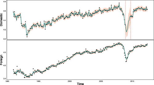
The left panel of Figure 13 zooms into the upper panel of Figure 12. The corresponding right panel shows the estimated free-rider effect (blue bars) as percentage share of domestic vehicle orders between 01/2009 and 09/2009. The mean value for the free-rider effect over time is 96.88% of domestic vehicle sales during the existence of the program. Thus, the program actually “created” additional purchases of domestic cars amounting to about 3.12% of observed sales figures during the transitory subsidization period. This figure has to be seen against the backdrop of the fact that under the German scrapping scheme—similar to the US CARS program—roughly 60 percent of subsidized purchases were foreign brands (Schweinfurth 2009, p. 4).

Figure 13. Zoom into upper panel of Figure 12 and estimated “free-rider” effect (blue bars) as percentage share of domestic vehicle orders: 01/2009 to 09/2009 Note: The ineffective part of the scrapping bonus (“free-rider” effect) is calculated based on Kalman filter values.

The estimated net effect of the scrapping subsidy in the automobile sector is plotted in Figure 14. It is based on comparing the intervention model used in Section 3.5 including policy and crisis with an identical model excluding the policy and fitted to the counterfactual series derived above. The net effect is the difference in the two implied filters. For details see Appendix A.11.

Figure 14. Distortionary effects of product-specific subsidy within automobile sector Note: Automobile sector; estimated net effect of subsidy is computed as difference of estimated crisis effect based on intervention model as outlined in section 3.5 and an intervention model without policy function fitted to counterfactual series.

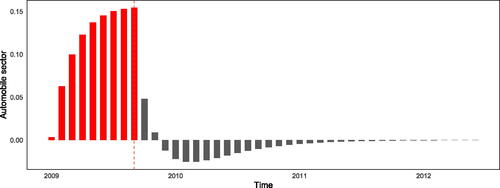
The black part in Figure 14 is the estimated negative net effect of the scrapping bonus resulting from a prolongation of the crisis effect due to structural disruptions in the automobile industry. “Front-loading” of vehicle expenditures and possibly also by subsidy-induced preference bias within the automobile sector implied a large proportion of acquired new cars and in turn a decrease in orders, production, and sales of new cars after the end of the scrapping bonus. Notably, the combined negative effect is smaller than the combined positive effect indicating a positive net effect for the automobile sector. This finding has to be assessed against the backdrop of the effect of the policy on other manufacturing sectors. This will be done in the next section.

Adda and Cooper (2000) have estimated a remarkably similar effect on expected aggregate vehicle sales following the scrapping bonuses introduced by French politicians Éduard Balladure and Alain Juppé in 1994/95 in France. Their findings for the policy effect on vehicle sales, which result from the simulation of a dynamic stochastic discrete choice model, look similar to our estimated net effect of the scrapping bonus in Germany. This especially applies to the part associated with the negative effect of the bonus on vehicle sales after the end of the policy. That is the black part in Figure 14. Thus, based on prior research, political decision-makers in Germany could have foreseen, at least in part, this negative externality of the scrapping bonus.

3.10. Substitution effect

Section 3.6 already identified an intersectoral substitution effect. Although the attribution of positive effects of the scrappage policy to the car sector is stable over different specifications, the same is not true for the attribution of negative or even positive effects of the subsidy to other manufacturing sectors.²⁴ Presumably these spillovers are negative and quantitatively smaller when compared to the positive effects for the automobile industry. A precise estimation and separation seems much harder in the first than in the latter case. We complement our previous approach by creating counterfactual series for the remaining sectors and proceed in a similar fashion as with the automobile industry.

For this purpose, we calculate the net effect of the subsidy again using the procedure described above. For the observed series, we rely on the same models and estimates as in Section 3.4. We include a policy transfer function as specified in Tables A.4 and A.5. This is justified as we assume to have found appropriate models capturing the true underlying processes. However, we suspect at least parts of the policy effects have been absorbed by the crisis transfer function.

The counterfactual series is derived in the same way as in the automobile industry. We replace the imposed missing values during the policy—01/2009 to 09/2009—with corresponding Kalman filter values (see Figure A.8 in Appendix A.10).²⁵ For each sector, we fit an identical or equivalent model to the counterfactual series. Both models differ only if the original one includes a policy transfer function, which then is excluded for the counterfactual series. The net effect of the subsidy is computed as the difference of the estimated stylized crisis effect from both models.

The resulting net effect, summed up over all sectors except the automobile and vehicles other than cars²⁶ industries is given in Figure 15. Overall, we see a sizable negative effect of the policy on other manufacturing industries during and after the program. Only with a delay of six up to 18 months does the effect turn positive. The estimates support the finding from Section 3.6 of an intersectoral bias. Beyond that, we find indications of somewhat delayed pent-up demand effects in the aftermath of the scrappage scheme.²⁷

Figure 15. Distortionary effects of product-specific subsidy within automobile sector Note: Automobile sector; estimated net effect of subsidy is computed as difference of estimated crisis effect based on intervention model as outlined in Section 3.5 and an intervention model without policy function fitted to counterfactual series.

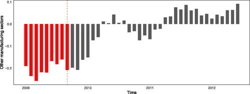
Relating these findings to the ones from the automobile sector shows that the policy is not neutral in this dimension. While the overall effect in the automobile sector is estimated positive, the overall effect in the other sectors is negative. Together with the relatively low intertemporal bias within the car sector, this indicates a dynamically not compensated shift of demand due to the policy. In other words: the scrappage scheme shifts demand to the automobile sector at the expense of the other manufacturing sectors.

Finally, it should again be stressed that our approach isn’t yet firmly based on the potential outcomes model and that our interpretation is therefore rather quasi-causal. Although we assume that our counterfactual series capture the sectoral behavior of domestic orders in the absence of the scrappage premium and that our analysis therefore estimates the effect of this policy, we admit that such an interpretation is necessarily tentative and preliminary.

4. Discussion

Many countries temporarily subsidize specific products to cushion the effects of an overall downturn in economic activity or to meet the aims of specific lobbying groups. Generally, such measures may boost sales in the short run. However, there might be intersectoral distortions through crowding out demand for other products as well as intertemporal distortions due to the temporary nature of such programs shifting purchases from the future to the present and possibly reversing the surge in sales after the end of the measure. The latter is referred to as program reversal or payback effect and cannot be quantified in terms of size and timing relying on standard time series techniques such as sales projections based on error correction models; see, e.g. Haugh et al. (2010). In general, the existing literature does not provide a coherent analytical framework to disentangle and quantify intersectoral as well as intertemporal (payback and rebound) distortions and to assess the effectiveness of such measures.

We show how such an assessment can be done using intervention analysis à la Box and Tiao (1975). Beyond this, we propose a complementary framework based on Kalman filtered estimates of counterfactual time series using information contained in series unaffected by the intervention and on netting out corresponding factual and counterfactual response functions.

In our empirical application, we study the largest car scrappage scheme in recent history installed by the German government between January and September 2009. In contrast to the perception of the scheme having substantially contributed to the stabilization of one of the European core industries, we find the demand-sided effectiveness of such a temporary product-specific subsidy to be rather poor. According to our estimates, the program created additional purchases of domestic products amounting to just about three percent of observed sales figures. Thus, buyers realized substantial unintended windfall gains that are as opposed to implications of alternatives, such as e.g., governmental sales and re-sales on the secondary market, not or less neutral with regard to the public budget. Additionally, stabilization comes, according to our estimates, at the price of a prolongation of the sectoral trough and a retardation of the subsequent recovery in the automobile industry by more than one year.

These are non-trivial costs given that the annual turnover of the automobile industry amounts to ten percent of German GDP. Furthermore and in line with basic theory, we find evidence for net sectoral crowding out and intersectoral bias of the measure concerning the vast majority of competing industries in the manufacturing sector. It might have been avoided resorting to alternative measures such as consumption vouchers with deadlines. The latter are also less prone to distributive bias, inasmuch as they do not discriminate against non-beneficiaries as is the case for households who cannot afford to buy new cars in case of scrappage programs.

Regarding the technical aspect of our analysis, both our methods have shown some limitations. Intervention models are flexible enough to accommodate multiple interventions. However, the disentanglement of their individual effects, which necessarily rests on specific functional form assumptions, hinges on the interconnection of both effects. When both are sizable and of opposite character, their identification works comparatively well. However, if both effects run together and are of unequal size, results are much less stable and probably notoriously incomplete. Building counterfactuals promises a remedy but hinges crucially on underlying identifying assumptions. Consequently, we propose a toolkit that has to be used carefully and with discretion. In cases in which no comparison is possible due to all relevant units being treated, intervention analysis and separation of contributions of individual interventions offer a way out. When multiple interventions do not affect all units, netting out corresponding factual and counterfactual response functions seems promising. Especially in the case of multiple interventions of unequal size and identical effective direction.

However, to convert our eclectic and still provisional approach into a more firmly established systematic approach for causal analysis, we need to develop a more refined theoretical framework and connect it to the well-established potential outcomes model. Although our approach is not yet fully backed up by such a precise analytical setup, we are still convinced that it constitutes a valuable tool that can produce relevant insights and findings. The sensibility and plausibility of our general results underline our perspective.

5. Conclusion

Analyzing the German car scrappage scheme 2009, we find little evidence of neutrality. Though we can confirm demand-sided effectiveness, our analysis shows both intertemporal and intersectoral bias. The resulting distortions are larger than the short-lived positive effects and exhibit a notable inertia.

In sum, our findings support the recent view of the quantitative theoretical literature that calls the usefulness of national policies to temporarily protect particular domestic industries into question by showing that they also induce technology bias favoring products of dated technology such as diesel engines (Miravete et al. 2018).

Acknowledgments

We thank the editor-in-chief, Milan Stehlik, two anonymous referees, Jesus Crespo Cuaresma, Christian Hutter, Christian Merkl, Willi Semmler, Thomas Steger, Roman Stöllinger, Marco Sunder, Timo Trimborn, Enzo Weber, and participants of the IWH Workshop on Fiscal Policy and the Great Recession, of the Recent Developments in Macroeconomics Conference at ZEW Mannheim, the ‘Modelling regime changes’ session of the International Conference on Computational and Financial Econometrics (CFE), and of seminars at Vienna University of Economics and Business, IAB/University of Erlangen-Nuremberg, and the University of Leipzig for many valuable comments and suggestions.

Disclosure statement

No potential conflict of interest was reported by the author(s).

Notes

1. However, in international terms, the dip was rather modest. Only car sales growth in Poland and China reacted even less negatively than the German one from 09/08 to 01/09; see Haugh et al. (2010, p. 95).

2. Ultimately, the circumstances allow only for a net effect to be quantified. We are indebted to one of the anonymous referees for drawing our attention to this aspect.

3. In the simple underlying model detailed in the Appendix this is due to Equation (A.1.9(A.1.9) $$\begin{array}{l}\frac{dV}{ds}=p{f}^{\prime }\frac{d{R}_x}{ds}+\underset{>0}{\underbrace{(g^{\prime }-k^{\prime })}}\frac{d{R}_y}{ds}.\end{array}$$(A.1.9) ).

4. Only recently, Menchetti et al. (2022) proposed a refined framework similar to intervention analysis by Box and Tiao (1975) but anchored in the potential outcomes framework. Like intervention analysis, their approach is based on ARIMA models and is therefore suited to complement existing methodologies like DiD or synthetic controls.

5. The demarcation between ITS analysis and intervention analysis in the sense of Box and Tiao (1975) is not clear-cut. For example, Schaffer et al. (2021) acknowledge that ITS traditionally uses segmented regression which may limit applications in case of time series with a more complex autocorrelative structure. They propose to augment ITS by allowing ARIMA components and transfer functions. Although they do not mention Box and Tiao (1975), the proposed approach is more like intervention analysis than traditional ITS and blends both methods.

6. We choose June 2012 as endpoint of our sample period as it generally marks a point of discontinuation of the official statistics on industrial new orders and corresponding sectoral series in European countries. See de Bondt et al. (2013) for detail.

7. Different from the situation at the time in the US, where subprime auto credit had been unsustainably inflated by the preceding housing and credit bubble (Goolsbee and Krueger 2015), neither credit crunch in the sense of households lacking access to credit and, thus, postponing car purchases nor the liquidation risk of the “big 3” car producers were given for Germany (Haugh et al. 2010).

8. Parameter estimates are obtained by Maximum Likelihood (ML) estimation.

9. It is noteworthy in this context that the German scrappage scheme preceded all comparable temporary programs in the OECD apart from the one installed in France. However, the latter represents the smallest among the five largest schemes for 2009 amounting to less than 8 percent of the German subsidization (Schweinfurth 2009; Haugh et al. 2010).

10. The impact of relying on the AIC instead of, for example, the BIC is shown in Figures A.5, A.6, and A.7 in Appendix A.9.

11. Considering only periods around the crisis, it looks as if the domestic textile sector was affected permanently. However, Figure 3 reveals the series has returned to its long-run trend.

12. This result is somewhat sensitive with regard to the underlying noise model. When repeating this step with a BIC-based noise model, we find the clothing, electronics, cars, pharmaceutics, machines, and other vehicles sectors to be significantly affected by the policy. See Appendix A.9.

13. The null of the model capturing the dependence structure of the time series cannot be rejected at a 5% level of significance in all but four cases.

14. As can be seen, foreign orders in the pharmaceutics sector declined already in 08/2007 while unaffected by later crisis events.

15. A graphical depiction of sample autocorrelation functions and residual histograms, given in Figures A.1 and A.2 in Appendix A.7, underscores this argument. Moreover, Figures A.3 and A.4 in Appendix A.8 show the model results when shifting the intervention period to 08/2007 – 08/2008 and analyzing the financial crisis directly. Qualitatively different from the aftermath of the Lehman Brothers collapse in September 2008, the German economy before appeared to be flourishing rather than declining.

16. To get an impression see the upper left panel in Figure A.5.

17. The positive part in the lower right panel in Figure 9 is not robust against changes in the noise model. The negative finding of a lasting negative effect, however, is still supported; see Figure A.6 in Appendix A.9.

18. This is closely linked to a “free-rider” problem, which we describe in more detail later.

19. Microeconomically, one route of reasoning for the substantially delayed rebound of consumer demand for autos might be that some households planned the acquisition of two low-price segment products for 2010 or later, and due to the subsidy not only pulled forward their purchasing but also changed their plan to acquire only one (subsidized) product from the premium price-segment. However, this contrasts with international experience suggesting a boost of low-margin segments (Haugh et al.2010). Our volume index series does not allow us to test such hypotheses.

20. Although we use the terms “counterfactual,” “effect,” and “impact,” it should be kept in mind that this is kind of a stretch. Since our analytical approach is not firmly grounded in an established causal framework, we basically borrow this wording to formulate our interpretation.

21. Thus, the values for the missing observations are estimated using the Kalman filter by making use of the information incorporated in a second series, i.e., foreign orders, which is assumed to be related to the series with missing observations. This method is advocated by Harvey and Chung (2000).

22. Note, since we do not use the Kalman Smoother at any point, our approach does not violate the non-anticipation assumption of casual analysis (Rubin 1978). Other than the Kalman Smoother, the Kalman filter always uses past and present observed values only; see Appendix A.13.2.

23. The superscript (.) ^(F) denotes Kalman filter values.

24. Compare, for example, Figure A.5 and A.6 in Appendix A.9 with Figures 8 and 9.

25. We can state that both models use the same underlying noise model n_t as all data points except for the ones between January and September 2009 are identical. Moreover, by limiting the artificially created gap of missing values to the period from January to September 2009, we also exclude the onset of the European debt crisis as a potential confounder.

26. The results in this sector are implausible, see Figure A.9 in Appendix A.11.

27. Above results are based on stretching the argument on the mirror image property of foreign and domestic orders in the automobile sector.

Appendix A

A

A.1. Model motivating Figure 2

Let the model economy consist of a sector x and all remaining industries y, where sector x is subsidized. The two divisions produce with production functions (A.1.1) $$\begin{array}{l}x=f(R_x);f^{\prime }>0\text{, }{f}^{\prime \prime }<0\end{array}$$(A.1.1) (A.1.2) $$\begin{array}{l}y=g(R_y);g^{\prime }>0\text{, }{g}^{\prime \prime }<0,\end{array}$$(A.1.2) where R denotes resources of any kind. In equilibrium the following three conditions need to hold (A.1.3) $$\begin{array}{ll}(p+s)f^{\prime }(R_x)& =m_x^0\end{array}$$(A.1.3) (A.1.4) $$\begin{array}{ll}{g}^{\prime }(R_y)& =m_y\end{array}$$(A.1.4) (A.1.5) $$\begin{array}{ll}{m}_y-c& =\pi m_x^0+(1-\pi )\alpha ,\end{array}$$(A.1.5) i.e., input factors in y (for which the price is normalized to unity) are rewarded their marginal product m. The same applies for sector x; however, market price p is upwardly biased by a (scrappage) subsidy amounting to s. In Equation (A.1.5(A.1.5) $$\begin{array}{ll}{m}_y-c& =\pi m_x^0+(1-\pi )\alpha ,\end{array}$$(A.1.5) ) c are costs of any kind due to resources shifting from one part of the economy to another, π is the probability of resources being used for production in sector x, α is the alternative use value of resources spent in sector x. Equation (A.1.5(A.1.5) $$\begin{array}{ll}{m}_y-c& =\pi m_x^0+(1-\pi )\alpha ,\end{array}$$(A.1.5) ) ensures that in equilibrium there is no flow of resources from all other sectors y into x and vice versa. π is given by (A.1.6) $$\begin{array}{l}\pi =\frac{R_x}{R_0-R_y},\end{array}$$(A.1.6) where R₀ is the total amount of resources in the model economy. Obviously, if π < 1 there are some resources unused. By simple logics, we can already say that in case the subsidization of sector x ends, R_x should decrease. As π decreases (A.1.7) $$\begin{array}{l}{m}_y-c>\pi m_x^0+(1-\pi )\alpha ,\end{array}$$(A.1.7) mobile resources are drawn from sector x into remaining sectors y. As a consequence m_y will have to decrease in order for the economy to reach a new equilibrium.

In the following, we will briefly consider the effects of a variation in s. What are the social effects of a variation of s? Social benefits are given by (A.1.8) $$\begin{array}{l}V=pf(R_x)+g(R_y)-k(R_y-R_y^0).\end{array}$$(A.1.8)

The subtractive part in (A.1.8(A.1.8) $$\begin{array}{l}V=pf(R_x)+g(R_y)-k(R_y-R_y^0).\end{array}$$(A.1.8) ) represents adjustment costs that are due to sectorally shifting resources. These costs represent social costs of any kind. Hence, the (gross) effect of a variation in s is given by (A.1.9) $$\begin{array}{l}\frac{dV}{ds}=p{f}^{\prime }\frac{d{R}_x}{ds}+\underset{>0}{\underbrace{(g^{\prime }-k^{\prime })}}\frac{d{R}_y}{ds}.\end{array}$$(A.1.9)

In order to isolate the effects of a variation in s we need to quantify dR_x∕ds and dR_y∕ds first. Thus, we need to consider all three equilibrium conditions. For the first condition, we obtain (A.1.10) $$\begin{array}{l}(p+s)f^{\prime \prime }d{R}_x+f^{\prime }ds=0\Rightarrow \frac{d{R}_x}{ds}=-\frac{f^{\prime }}{(p+s)f^{\prime \prime }}=\beta >0.\end{array}$$(A.1.10)

It is slightly more complicated to calculate dR_y∕ds. First, it requires the total derivative of the second equilibrium condition, which is simply given by (A.1.11) $$\begin{array}{l}{g}^{\prime \prime }d{R}_y=d{m}_y.\end{array}$$(A.1.11)

Second, considering the total derivative of the third equilibrium condition implies (A.1.12) $$\begin{array}{ll}d{m}_y& =(m_y^0-\alpha )d\pi ={\delta }_{x}d\pi .\end{array}$$(A.1.12)

Substituting (A.1.12(A.1.12) $$\begin{array}{ll}d{m}_y& =(m_y^0-\alpha )d\pi ={\delta }_{x}d\pi .\end{array}$$(A.1.12) ) into (A.1.11(A.1.11) $$\begin{array}{l}{g}^{\prime \prime }d{R}_y=d{m}_y.\end{array}$$(A.1.11) ), we are given (A.1.13) $$\begin{array}{l}{g}^{\prime \prime }d{R}_y={\delta }_{x}d\pi .\end{array}$$(A.1.13)

From (A.1.6(A.1.6) $$\begin{array}{l}\pi =\frac{R_x}{R_0-R_y},\end{array}$$(A.1.6) ) we see that (A.1.14) $$\begin{array}{ll}d\pi & =\frac{(R_0-R_y)d{R}_x-R_x(-d{R}_y)}{(R_0-R_y{)}^2}=\frac{(R_0-R_y)d{R}_x+R_{x}d{R}_y}{(R_0-R_y{)}^2}\\ & =\frac{d{R}_x}{R_0-R_y}+\frac{R_x}{R_0-R_y}\cdot \frac{d{R}_y}{R_0-R_y}=\frac{d{R}_x}{R_0-R_y}+\frac{\pi d{R}_y}{R_0-R_y}.\end{array}$$(A.1.14)

Combining (A.1.13(A.1.13) $$\begin{array}{l}{g}^{\prime \prime }d{R}_y={\delta }_{x}d\pi .\end{array}$$(A.1.13) ) and (A.1.12(A.1.12) $$\begin{array}{ll}d{m}_y& =(m_y^0-\alpha )d\pi ={\delta }_{x}d\pi .\end{array}$$(A.1.12) ) results in (A.1.15) $$\begin{array}{l}{g}^{\prime \prime }d{R}_y={\delta }_x\frac{d{R}_x}{R_0-R_y}+{\delta }_x\frac{\pi d{R}_y}{R_0-R_y}\iff \\ (g^{\prime \prime }-{\delta }_x\frac{\pi }{R_0-R_y})d{R}_y=\frac{{\delta }_x}{R_0-R_y}d{R}_x\end{array}$$(A.1.15)

Relationship (A.1.10(A.1.10) $$\begin{array}{l}(p+s)f^{\prime \prime }d{R}_x+f^{\prime }ds=0\Rightarrow \frac{d{R}_x}{ds}=-\frac{f^{\prime }}{(p+s)f^{\prime \prime }}=\beta >0.\end{array}$$(A.1.10) ) allows to substitute dR_x by βds and, hence, (A.1.16) $$\begin{array}{l}d{R}_y=\frac{{\delta }_x\beta ds}{(g^{\prime \prime }-\frac{{\delta }_x\pi }{R_0-R_y})(R_0-R_y)}\Rightarrow \frac{d{R}_y}{ds}=\gamma <0\end{array}$$(A.1.16)

We now know the respective signs of dR_x∕ds and dR_y∕ds. Thus, based on Equation (A.1.9(A.1.9) $$\begin{array}{l}\frac{dV}{ds}=p{f}^{\prime }\frac{d{R}_x}{ds}+\underset{>0}{\underbrace{(g^{\prime }-k^{\prime })}}\frac{d{R}_y}{ds}.\end{array}$$(A.1.9) ), it can be stated that in case s is decreased resources (and thus output) in sector x will decrease. However, this may, at least partly, be compensated by resources drawn into and output produced in sector y. If the first additive part of (A.1.9(A.1.9) $$\begin{array}{l}\frac{dV}{ds}=p{f}^{\prime }\frac{d{R}_x}{ds}+\underset{>0}{\underbrace{(g^{\prime }-k^{\prime })}}\frac{d{R}_y}{ds}.\end{array}$$(A.1.9) ) is larger than the second one, there will be inefficiency in the sense of unused resources.

These qualitative results are summarized graphically in Figure 2 in the text.

A.2. Coding of variables and descriptive statistics

Table A.1. Coding of variables. Descriptions, NACE codes and descriptive statistics for economic sectors’ foreign and domestic new orders.

Industry	Industry Number	NACE ’08 (2-digits code)	Series	Series Name	Min	Max	Mean	SD
Electronical/optical devices	Manuf. of computer,electronic and optical products	26	orders inl(and)	OIElinl	54.20	173.20	95.30	33.38
			orders for(eign)	OIElfor	33.70	166.90	79.16	35.06
Clothing	Manufacture of wearing apparel	14	orders inl	OIClinl	57.10	241.70	122.62	41.85
			orders for	OIClfor	71.10	173.90	98.42	16.88
Chemicals	Manufacture of chemicals and chemical products	20	orders inl	OIChinl	77.40	109.30	97.81	5.30
			orders for	OIChfor	58.20	115.80	85.11	14.75
Electronics	Manufacture of electrical equipment	27	orders inl	OIEdinl	75.00	141.00	99.67	8.73
			orders for	OIEdfor	43.90	145.00	84.35	24.54
Cars	Manuf. of motor vehicles, trailers, semi-trailers	29	orders inl	OICainl	57.20	117.80	89.59	12.07
			orders for	OICafor	34.40	129.00	78.15	28.45
Metalworking	Manuf. of fabricated metal products, ex. machinery	25	orders inl	OIMeinl	81.00	122.30	99.86	9.25
			orders for	OIMefor	44.90	139.60	82.15	25.70
Production of paper	Manufacture of paper and paper products	17	orders inl	OIPainl	86.20	112.20	97.97	6.34
			orders for	OIPafor	47.10	118.10	83.84	21.04
Pharmaceutics	Manuf. of basic pharmaceutical products and prep.	21	orders inl	OIPhinl	71.40	117.40	89.03	8.45
			orders for	OIPhfor	28.60	130.90	77.52	28.60
Textiles	Manufacture of textiles	13	orders inl	OITxinl	73.20	221.40	126.93	36.08
			orders for	OITxfor	75.50	109.10	94.59	7.79
Machines	Manufacture of machinery and equipment n.e.c.	28	orders inl	OIMainl	65.70	131.70	97.85	11.84
			orders for	OIMafor	50.40	143.70	84.58	25.05
Production of metal	Manufacture of basic metals	24	orders inl	OIStinl	59.40	148.70	102.33	11.03
			orders for	OIStfor	54.90	120.20	85.87	15.33
Vehicles other than cars	Manufacture of other transport equipment	30	orders inl	OIBoinl	42.10	508.10	88.55	45.94
			orders for	OIBofor	12.30	294.10	74.89	48.88

A.3. Lag selection for noise model n_t

Table A.2. Lag order selection for noise model based on minimizing different information criteria.

Industry No.	Series name	AIC	LB	BIC	LB	AICC	LB
26	OIElinl	(0,1,1)	0.3717	(0,1,1)	0.3717	(0,1,1)	0.3717
	OIElfor	(0,1,2)*	0.3222	(1,1,0)	0.0945	(0,1,2)*	0.3222
14	OIClinl	(1,1,2)*	0.9932	(0,1,1)*	0.9223	(1,1,2)*	0.9932
	OIClfor	(2,1,3)	0.6545	(0,1,2)	0.1257	(2,1,3)	0.6545
20	OIChinl	(2,1,3)	0.3903	(1,1,0)	0.1214	(2,1,3)	0.3903
	OIChfor	(1,1,0)*	0.1248	(1,1,0)	0.1398	(1,1,0)*	0.1248
27	OIEdinl	(2,1,0)	0.0134	(2,1,0)	0.0134	(2,1,0)	0.0134
	OIEdfor	(4,1,1)*	0.3248	(0,1,1)*	0.0188	(4,1,0)*	0.3469
29	OICainl	(0,1,1)	0.6884	(0,1,1)	0.6884	(0,1,1)	0.6884
	OICafor	(2,1,0)*	0.9894	(2,1,0)*	0.9894	(2,1,0)*	0.9894
25	OIMeinl	(2,1,1)	0.4441	(1,1,0)	0.2083	(2,1,1)	0.4441
	OIMefor	(1,1,1)*	0.5598	(0,1,1)*	0.5946	(0,1,1)*	0.5946
17	OIPainl	(0,1,1)	0.8908	(0,1,1)	0.8908	(0,1,1)	0.8908
	OIPafor	(0,1,1)*	0.1300	(0,1,1)	0.1489	(0,1,1)*	0.1300
21	OIPhinl	(0,1,3)	0.8585	(0,1,1)	0.5995	(0,1,3)	0.8585
	OIPhfor	(2,1,3)*	0.3834	(3,1,1)*	0.1898	(2,1,3)*	0.3834
13	OITxinl	(2,1,0)*	0.8766	(0,1,1)*	0.8073	(2,1,0)*	0.8766
	OITxfor	(2,1,0)	0.0688	(1,1,0)	0.0353	(2,1,0)	0.0688
28	OIMainl	(3,1,2)*	0.1856	(0,1,1)	0.0590	(3,1,2)*	0.1856
	OIMafor	(2,1,3)	0.9503	(1,1,2)	0.7549	(2,1,3)	0.9503
24	OIStinl	(2,1,2)	0.1858	(1,1,0)	0.0041	(2,1,2)	0.1858
	OIStfor	(0,1,1)	0.1596	(0,1,1)	0.1596	(0,1,1)	0.1596
30	OIBoinl	(2,1,1)	0.4574	(0,1,1)	0.0691	(2,1,1)	0.4574
	OIBofor	(0,1,1)*	0.6047	(0,1,1)	0.5650	(0,1,1)*	0.6047

Suggested (p,d,q)-order in parenthesis. Star denotes presence of drift parameter. LB-column shows p-value for Ljung-Box statistic (constructed on 20 lags) for suggested model (pre-crisis period 01/91 – 07/07).

A.4. Lag selection for crisis transfer function $m_t^C$

Table A.3. AIC for intervention models without scrappage program given different lag order specifications for transfer function.

NACE	domestic			foreign
Code	(0, 0)^C	(1, 0)^C	(2, 0)^C	(0, 0)^C	(1, 0)^C	(2, 0)^C
26	− 705.653	-704.999	−703.673	−675.737	-677.163	-
14	−772.803	-790.568	−789.199	−376.623	-374.638	− 381.327
20	−1192.866	-1206.921	-	−1082.89	−1098.536	-1129.521
27	−765.637	−784.715	-807.774	−583.324	−581.762	-591.614
29	−847.336	-848.733	− 849.136	−757.867	−772.342	-810.941
25	−1126.444	-1143.87	−1138.95	−855.42	-872.378	−870.19
17	−1198.885	−1205.156	-1216.537	−929.869	-932.321	−930.033
21	−909.658	-916.154	−916.03	-581.781	-	-
13	−1157.244	−1171.233	-1174.895	−1036.934	−1048.758	-1061.573
28	−966.288	-994.004	-	-	-	-737.31
24	−832.531	−844.837	-871.387	−689.444	-697.838	−695.557
30	166.398	168.312	152.423	273.985	270.38	271.826

Minimum AIC for a given series is given in italics. Chosen specification is shown in bold. Deviations from minimum AIC as described in Sections 3.2 and 3.3. Empty cells indicate non-converging models.

A.5. Overview of intervention models

Table A.4. Intervention models fitted to log series.

NACE Code	Series name	Series	nt	$m_t^C$	$m_t^P$
26	OIEl	inl(and)	ARIMA(0,1,1)	$(\frac{{\omega }_0}{1-{\delta }_{1}L}){\eta }_t^{({\tau }_1,{\tau }_2)}$	-
		for(eign)	ARIMA(0,1,2)	$(\frac{{\omega }_0}{1-{\delta }_{1}L}){\eta }_t^{({\tau }_1,{\tau }_2)}$	-
14	OICl	inl	ARIMA(1,1,2)	$(\frac{{\omega }_0}{1-{\delta }_{1}L})L^3{\zeta }_t^{\tau }$	-
		for	ARIMA(2,1,1)	$(\frac{{\omega }_0}{1-{\delta }_{1}L})L^3{\zeta }_t^{\tau }$	-
20	OICh	inl	ARIMA(2,1,3)	$(\frac{{\omega }_0}{1-{\delta }_{1}L}){\eta }_t^{({\tau }_1,{\tau }_2)}$	-
		for	ARIMA(1,1,0)	$(\frac{{\omega }_0}{1-{\delta }_{1}L}){\eta }_t^{({\tau }_1,{\tau }_2)}$	-
27	OIEd	inl	ARIMA(2,1,0)	$(\frac{{\omega }_0}{1-{\delta }_{1}L-{\delta }_2{L}^2}){\eta }_t^{({\tau }_1,{\tau }_2)}$	$(\frac{{\omega }_1}{1-{\delta }_{3}L}){\eta }_t^{({\tau }_3,{\tau }_4)}$
		for	ARIMA(4,1,1)	$(\frac{{\omega }_0}{1-{\delta }_{1}L-{\delta }_2{L}^2}){\eta }_t^{({\tau }_1,{\tau }_2)}$
29	OICa	inl	ARIMA(0,1,1)	$(\frac{{\omega }_0}{1-{\delta }_{1}L}){\eta }_t^{({\tau }_1,{\tau }_2)}$	$(\frac{{\omega }_1}{1-{\delta }_{2}L}){\eta }_t^{({\tau }_3,{\tau }_4)}$
		for	ARIMA(2,1,0)	$(\frac{{\omega }_0}{1-{\delta }_{1}L}){\eta }_t^{({\tau }_1,{\tau }_2)}$	-
25	OIMe	inl	ARIMA(2,1,1)	$(\frac{{\omega }_0}{1-{\delta }_{1}L}){\eta }_t^{({\tau }_1,{\tau }_2)}$	-
		for	ARIMA(1,1,1)	$(\frac{{\omega }_0}{1-{\delta }_{1}L}){\eta }_t^{({\tau }_1,{\tau }_2)}$	-
17	OIPa	inl	ARIMA(0,1,1)	$(\frac{{\omega }_0}{1-{\delta }_{1}L-{\delta }_2{L}^2}){\eta }_t^{({\tau }_1,{\tau }_2)}$	-
		for	ARIMA(0,1,1)	$(\frac{{\omega }_0}{1-{\delta }_{1}L}){\eta }_t^{({\tau }_1,{\tau }_2)}$	-
21	OIPh	inl	ARIMA(0,1,3)	$(\frac{{\omega }_0}{1-{\delta }_{1}L}){\zeta }_t^{\tau }$	$(\frac{{\omega }_1}{1-{\delta }_{2}L}){\eta }_t^{({\tau }_3,{\tau }_4)}$
		for	ARIMA(2,1,3)	$(\frac{{\omega }_0}{1-{\delta }_{1}L}){\eta }_t^{({\tau }_1,{\tau }_2)}$	-
13	OITx	inl	ARIMA(2,1,0)	$(\frac{{\omega }_0}{1-{\delta }_{1}L-{\delta }_2{L}^2}){\eta }_t^{({\tau }_1,{\tau }_2)}$	-
		for	ARIMA(2,1,0)	$(\frac{{\omega }_0}{1-{\delta }_{1}L}){\zeta }_t^{\tau }$	-
28	OIMa	inl	ARIMA(3,1,2)	$(\frac{{\omega }_0}{1-{\delta }_{1}L}){\eta }_t^{({\tau }_1,{\tau }_2)}$	-
		for	ARIMA(2,1,3)	$(\frac{{\omega }_0}{1-{\delta }_{1}L}){\eta }_t^{({\tau }_1,{\tau }_2)}$	-
24	OISt	inl	ARIMA(2,1,2)	$(\frac{{\omega }_0}{1-{\delta }_{1}L-{\delta }_2{L}^2}){\eta }_t^{({\tau }_1,{\tau }_2)}$	$(\frac{{\omega }_1}{1-{\delta }_{3}L}){\eta }_t^{({\tau }_3,{\tau }_4)}$
		for	ARIMA(0,1,1)	$(\frac{{\omega }_0}{1-{\delta }_{1}L}){\eta }_t^{({\tau }_1,{\tau }_2)}$	-
30	OIBo	inl	ARIMA(2,1,1)	$(\frac{{\omega }_0}{1-{\delta }_{1}L}){\eta }_t^{({\tau }_1,{\tau }_2)}$	-
		for	ARIMA(0,1,1)	$(\frac{{\omega }_0}{1-{\delta }_{1}L-{\delta }_{2}L}){\eta }_t^{({\tau }_1,{\tau }_2)}$	-

Scrappage program is included in specification if model is significantly different from restricted model (see Table A.5). Superscripts C and P denote mean function specifications for financial crisis and scrappage program respectively.

A.6. Coefficient table

Table A.5. Estimated models based on AIC. ϕ_i denotes AR, θ_i MA, and τ drift parameters from the underlying noise model. ${\delta }_i^C$ denotes financial crisis AR, ${\omega }_i^C$ financial crisis MA, ${\delta }_i^P$scrappage program AR, and ${\omega }_i^C$ scrappage program MA coefficients from the intervention model. Standard errors are shown in parenthesis below. The last column shows p-values for Ljung-Box test statistic based on 20 Lags.

Series	ϕ1	ϕ2	ϕ3	ϕ4	θ1	θ2	θ3	τ	${\delta }_1^C$	${\delta }_2^C$	${\omega }_0^C$	${\delta }_1^P$	${\omega }_0^P$	AIC	LB
OIElinl					−0.4128				−0.8482		−0.0382			−704.9991	0.8195
					(0.0564)				(0.1559)		(0.0328)
OIElfor					−0.5346	0.1216		0.0041	0.7926		−0.0404			−677.1633	0.4574
					(0.0623)	(0.0608)		(0.0023)	(0.1287)		(0.0208)
OIClinl	−0.4626				−0.1542	−0.5092		−0.0038	0.5748		−0.0951			−794.1437	0.4696
	(0.1620)				(0.1452)	(0.1017)		(0.0008)	(0.1056)		(0.0252)
OIClfor	0.8718	−0.9375			−1.4900	1.3505	−0.5422		0.0322		−0.4296			−404.7196	0.9402
	(0.0468)	(0.0549)			(0.0913)	(0.1554)	(0.0829)		(0.2799)		(0.1163)
OIChinl	−0.9035	−0.9038			0.6870	0.7990	−0.0617		0.7798		−0.0399			−1206.9215	0.5010
	(0.0851)	(0.0644)			(0.1101)	(0.0731)	(0.0773)		(0.0582)		(0.0101)
OIChfor	−0.2942							0.0017	1.6985	−0.9108	−0.0322			−1129.5210	0.1923
	(0.0598)							(0.0013)	(0.0365)	(0.0326)	(0.0043)
OIEdinl	−0.7185	−0.3738							1.7256	−0.9381	−0.0380	0.9198	−0.0308	−811.7597	0.0005
	(0.0582)	(0.0580)							(0.0225)	(0.0213)	(0.0054)	(0.0771)	(0.0120)
OIEdfor	−0.2307	−0.1700	−0.0386	−0.2127	−0.4186			0.0033	0.2728	0.5558	−0.0742			−591.6144	0.6559
	(0.2116)	(0.1452)	(0.1022)	(0.0679)	(0.2152)			(0.0016)	(0.3853)	(0.3531)	(0.0252)
OICainl					−0.4661				0.7730		−0.0845	0.6514	0.1069	−868.7223	0.7222
					(0.0600)				(0.0653)		(0.0180)	(0.1096)	(0.0222)
OICafor	−0.5932	−0.3053						0.0040	1.7611	−0.9699	−0.0449			−810.9408	0.9634
	(0.0603)	(0.0602)						(0.0016)	(0.0200)	(0.0185)	(0.0050)
OIMeinl	0.6994	0.2041			−0.9652				0.8196		−0.0513			−1143.8700	0.1581
	(0.0686)	(0.0638)			(0.0292)				(0.0485)		(0.0104)
OIMefor	−0.0958				−0.3194			0.0029	0.8148		−0.0678			−872.3785	0.8713
	(0.1625)				(0.1564)			(0.0017)	(0.0555)		(0.0152)
OIPainl					−0.4873				1.7206	−0.9025	−0.0123			−1216.5368	0.8203
					(0.0568)				(0.0716)	(0.0658)	(0.0031)
OIPafor					−0.3045			0.0029	0.7618		−0.0312			−932.3213	0.2612
					(0.0613)			(0.0017)	(0.1100)		(0.0151)
OIPhinl					−0.5147	−0.1724	0.1034		0.9198		−0.0249	0.4470	−0.0429	−921.7465	0.7099
					(0.0628)	(0.0715)	(0.0609)		(0.0572)		(0.0128)	(0.2271)	(0.0211)
OIPhfor	−0.8363	−0.7576			−0.1062	−0.0074	−0.2398	0.0048	0.0005		0.0005			−581.7806	0.3870
	(0.0809)	(0.0739)			(0.1118)	(0.1040)	(0.0897)	(0.0012)	(0.0319)		(0.0319)
OITxinl	−0.3740	−0.1702						−0.0040	−0.0256	0.7092	−0.0658			−1174.8947	0.8222
	(0.0616)	(0.0615)						(0.0010)	(0.0825)	(0.0828)	(0.0120)
OITxfor	−0.4932	−0.1122							1.4680	−0.6568	−0.0434			−1061.4025	0.0477
	(0.0626)	(0.0631)							(0.0897)	(0.0835)	(0.0095)
OIMainl	−1.7256	−0.8969	−0.1069		1.4964	0.5408		−0.0005	0.8728		−0.0752			−994.0037	0.6988
	(0.5886)	(0.7149)	(0.1959)		(0.5813)	(0.5397)		(0.0017)	(0.0312)		(0.0120)
OIMafor	−1.5047	−0.5827			1.0144	−0.0664	−0.1623		1.3460	−0.4793	−0.0553			−737.3104	0.7866
	(0.4174)	(0.3797)			(0.4332)	(0.2007)	(0.2143)		(0.2075)	(0.1910)	(0.0183)
OIStinl	−0.7100	−0.9454			0.6279	1.0000			1.7818	−0.9789	−0.0541	−0.5003	0.0804	−877.0689	0.0357
	(0.0227)	(0.0215)			(0.0144)	(0.0237)			(0.0238)	(0.0232)	(0.0075)	(0.1261)	(0.0248)
OIStfor					−0.3568				0.7174		−0.0833			−697.8380	0.0212
					(0.0575)				(0.0838)		(0.0251)
OIBoinl	0.0775	0.1449			−0.9660				−0.7084	−0.9985	0.2603			152.4230	0.1931
	(0.0645)	(0.0642)			(0.0166)				(0.0255)	(0.0396)	(0.1189)
OIBofor					−0.9023			0.0058	0.8653		−0.1066			270.3802	0.5610
					(0.0338)			(0.0026)	(0.0642)		(0.0401)

A.7. Intervention model robustness plots

Figure A.1. Sample autocorrelation functions (SACF) for residuals from estimated intervention models for up to 40 lags (underlying specification given in Table A.5).

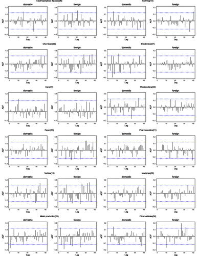
Figure A.2. Histogram and kernel density estimate for residuals (blue solid line) from estimated intervention models for up to 40 lags (underlying specification given in Table A.5). The red solid line shows a normal distribution using the residuals’ mean and standard deviation.

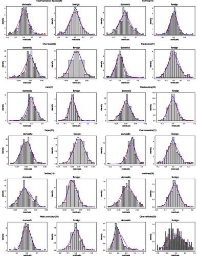
A.8. Financial crisis intervention 08/2007 – 08/2008

Figure A.3. Logarithm of original (solid line) and predicted values (dotted line) plus stylized crisis reactions for domestic new orders. Crisis is modeled as an extended impulse function with lag polynomial order r = 1 and s = 0 for δ(L) and ω(L).

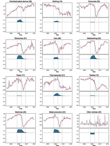
Figure A.4. Logarithm of original (solid line) and predicted values (dotted line) plus stylized crisis reactions for foreign new orders. Crisis is modeled as an extended impulse function with lag polynomial order r = 1 and s = 0 for δ(L) and ω(L).

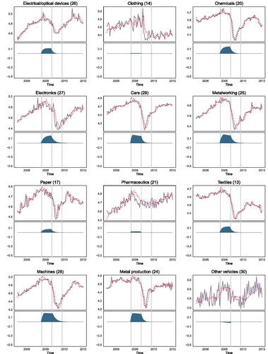
A.9. BIC-based analysis

To assess the impact of the utilized AIC-based lag-selection procedure on our findings, we repeat the analysis using the BIC. It guides selection of a noise model, while the transfer function is ultimately determined via likelihood ratio tests (see Section 3.2). The changes in the results are minor but reveal an important insight: while the stylized total sectoral dip functions are basically the same, attribution of the effects of the program to specific sectors as well as its quantification vary significantly.

Figure A.5. Stylized sectoral dips for BIC-based intervention models with significant effect of crisis and policy. Red area shows estimated crisis, blue estimated policy effect. Violet area compares combined effect of policy and crisis to estimate the reduced intervention model without the policy function.

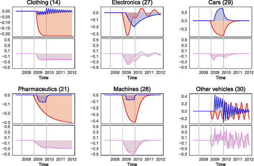
Figure A.6. Stylized sectoral dips for BIC based intervention models with significant effect of crisis and policy (exclusive sectors 14 and 30). Upper left panel shows other sector’s individual policy reactions. Upper right panel shows automobile sector’s policy reaction. Lower left panel shows total of other sector’s effects. Lower right panel shows total effect in car sector (yellow), non-car sector (green) and the net effect their difference (grey).

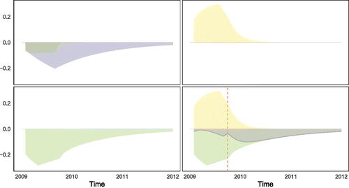
Figure A.7. Original and predicted series plus stylized sectoral dip functions from BIC based intervention models. Scrappage program is included for sectors $2,4,5,8,10,12$. Solid line shows logarithm of raw data, red dotted line fitted values. Grey vertical lines mark 08/2007, 09/2008, and 10/2009. Estimates for automobile (29) and other vehicle (30) sectors are identical to their AIC based estimates.

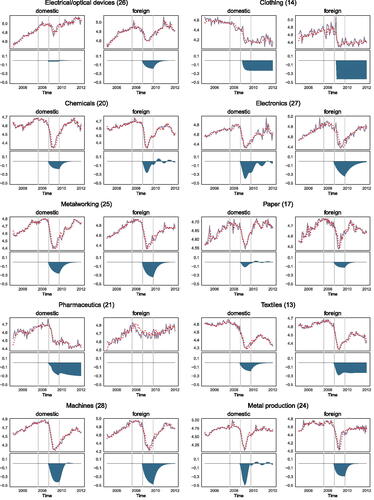
A.10. Kalman filter based counterfactual series

Figure A.8. Kalman filter-based counterfactual and original time series for logarithm of new orders with domestic origin. Dashed violet line shows observed, green solid line counterfactual time series. Red shaded area indicates 95% prediction interval. Vertical dashed red lines mark prediction period for imposed missing values. NACE sector numbers are in parenthesis.

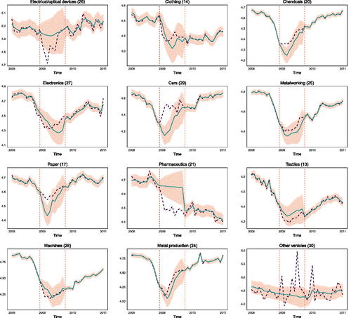
A.11. Kalman filter based sectoral net effects

Figure A.9. Kalman dilter-based comparison of implied filter for counterfactual and original time series for logarithm of new orders with domestic origin. Upper panel shows estimated effect for observed (violet) and augmented series (yellow). Lower panel shows net effect, i.e. difference between yellow and violet area from upper panel. Red part marks period of subsidy, black part time after. NACE sector numbers are in parenthesis.

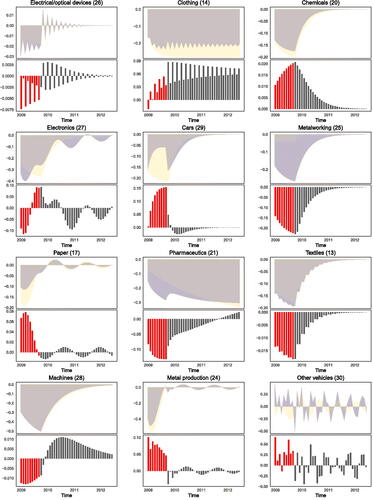
A.12. Additional plots

Figure A.10. Implied filter and model fit for other vehicles sector. Solid line shows logarithm of raw data, red dotted line fitted values. Grey vertical lines mark 08/2007, 09/2008, and 10/2009.

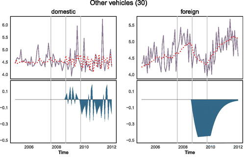
Figure A.11. Implied filter for strategic pull-forward effect model. Left panel shows cumulative effect, right and middle panels show underlying constituents. Blue area is related to scrappage program, red area to crisis.

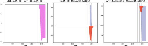
A.13. State-space models, Kalman filter, and model estimation

A.13.1. State-space models

A state-space model for a n-dimensional time series 𝒚_t consist of a measurement equation that relates the observed data to a m-dimensional state vector 𝜶_t. The generation of the state vector 𝜶_t from the past state 𝜶_t−1, for $t=1,...,T$, is determined by the state equation. The measurement equation has the form (A.13.1) $$\begin{array}{l}{\mathit{y}}_t={\mathit{Z}}_t{\mathit{\alpha }}_t+{\mathit{d}}_t+{\mathit{u}}_t,t=1,...,T.\end{array}$$(A.13.1)

In A.13.1(A.13.1) $$\begin{array}{l}{\mathit{y}}_t={\mathit{Z}}_t{\mathit{\alpha }}_t+{\mathit{d}}_t+{\mathit{u}}_t,t=1,...,T.\end{array}$$(A.13.1) 𝒁_t is an n×m matrix called measurement or observation matrix, 𝒅_t is an n×1 vector and ${\mathit{u}}_t\sim \text{iid }N(\mathbf{0},{\mathit{H}}_t)$ is an error vector. The state equation is given by (A.13.2) $$\begin{array}{l}{\mathit{\alpha }}_t={\mathit{T}}_t{\mathit{\alpha }}_{t-1}+{\mathit{c}}_t+{\mathit{R}}_t{\mathit{\nu }}_t,t=1,...,T.\end{array}$$(A.13.2)

In A.13.2(A.13.2) $$\begin{array}{l}{\mathit{\alpha }}_t={\mathit{T}}_t{\mathit{\alpha }}_{t-1}+{\mathit{c}}_t+{\mathit{R}}_t{\mathit{\nu }}_t,t=1,...,T.\end{array}$$(A.13.2) 𝑻_t is an m×m matrix called transition matrix, 𝒄_t is an m×1 vector, 𝑹_t is an m×g matrix and ${\mathit{\nu }}_t\sim \text{iid }N(\mathbf{0},{\mathit{Q}}_t)$ is a g×1 error vector. The matrices 𝒁_t, 𝒅_t, 𝑯_t, 𝑻_t, 𝒄_t, 𝑹_t and 𝑸_t are called system matrices. It is frequently assumed that the errors of the measurement and the transition equation are uncorrelated, i.e. $$\begin{array}{l}E[{\mathit{u}}_t{\mathit{\nu }}_t^{\prime }]=\mathbf{0}\mathrm{\forall }s,t=1,...,T.\end{array}$$

However, this assumption is not necessary; see Shumway and Stoffer (2011, p. 354–358) for a discussion of the case of correlated errors. Furthermore, it is assumed that the initial state is given by a normal vector $$\begin{array}{l}{\mathit{\alpha }}_0\sim N({\mathit{a}}_0,{\mathit{P}}_0);E[{\mathit{u}}_t{\mathit{a}}_0^{\prime }]=\mathbf{0},E[{\mathit{\nu }}_t{\mathit{a}}_0^{\prime }]=0,t=1,...,T.\end{array}$$

Note, that the model given in A.13.2(A.13.2) $$\begin{array}{l}{\mathit{\alpha }}_t={\mathit{T}}_t{\mathit{\alpha }}_{t-1}+{\mathit{c}}_t+{\mathit{R}}_t{\mathit{\nu }}_t,t=1,...,T.\end{array}$$(A.13.2) which includes only one lag, is not at all restrictive, as processes with higher orders may be casted into a state-space representation as well. Think for example, of an AR(2)-process $$\begin{array}{l}{y}_t={\varphi }_0+{\varphi }_1{y}_{t-1}+{\varphi }_2{y}_{t-2}+{\nu }_t,\text{with }{\nu }_t\sim \text{iid }N(0,{\sigma }^2).\end{array}$$

If we define ${\mathit{\alpha }}_t:=[y_t,y_{t-1}{]}^{\prime }$ the transition equation becomes $$\begin{array}{l}\left(\begin{array}{c}{y}_t\\ y_{t-1}\end{array}\right)=\left(\begin{array}{cc}{\varphi }_1& {\varphi }_2\\ 1& 0\end{array}\right)\left(\begin{array}{c}{y}_{t-1}\\ y_{t-2}\end{array}\right)+\left(\begin{array}{c}{\varphi }_0\\ 0\end{array}\right)+\left(\begin{array}{c}1\\ 0\end{array}\right){\nu }_t,\end{array}$$ whereas the measurement equation would be $$\begin{array}{l}{y}_t=[1,0]{\mathit{\alpha }}_t.\end{array}$$

Thus, the system matrices are $$\begin{array}{l}\mathit{T}=\left(\begin{array}{cc}{\varphi }_1& {\varphi }_2\\ 1& 0\end{array}\right),\mathit{R}=\left(\begin{array}{c}1\\ 0\end{array}\right),\mathit{c}=\left(\begin{array}{c}{\varphi }_0\\ 0\end{array}\right),Q={\sigma }^2,{\mathit{Z}}_t=[1,0],d_t=0,u_t=0\text{ and }\end{array}$$ $$\begin{array}{l}{H}_t=0.\end{array}$$

A.13.2. The Kalman filter procedure

In most cases the aim of any analysis based on a state-space model as defined by Equations (A.13.1(A.13.1) $$\begin{array}{l}{\mathit{y}}_t={\mathit{Z}}_t{\mathit{\alpha }}_t+{\mathit{d}}_t+{\mathit{u}}_t,t=1,...,T.\end{array}$$(A.13.1) ) and (A.13.2(A.13.2) $$\begin{array}{l}{\mathit{\alpha }}_t={\mathit{T}}_t{\mathit{\alpha }}_{t-1}+{\mathit{c}}_t+{\mathit{R}}_t{\mathit{\nu }}_t,t=1,...,T.\end{array}$$(A.13.2) ) will be to produce estimators for the underlying unobserved signal 𝜶_t given the data 𝒚_s, for $s=1,...,S$. Whenever s = t this problem is called filtering, while we speak of smoothing if s > t and forecasting in case s < t. The problem of finding such estimators is solved by the Kalman filter, Kalman Smoother, and forecasting recursions, respectively; see Petris et al. (2009, p. 53–72). In the following, we will focus on the derivation of the Kalman filter (i.e., s = t).

The Kalman filter is a set of recursion equations (prediction equations and updating equations) that determine the optimal estimates for the state vector 𝜶_t given the information available at time t (which we denote by I_t). The following definitions are used (A.13.3) $$\begin{array}{l}{\mathit{a}}_t:=E[{\mathit{\alpha }}_t|I_t]\end{array}$$(A.13.3) and (A.13.4) $$\begin{array}{l}{\mathit{P}}_t:=E[({\mathit{\alpha }}_t-{\mathit{a}}_t)({\mathit{\alpha }}_t-{\mathit{a}}_t{)}^{\prime }|I_t].\end{array}$$(A.13.4)

I.e., 𝒂_t is the optimal estimator of 𝜶_t based on I_t and 𝑷_t is the MSE matrix of 𝒂_t.

A.13.2.1. Prediction equations

Given 𝒂_t−1 and 𝑷_t−1 we get (A.13.5) $$\begin{array}{ll}{\mathit{a}}_{t|t-1}& =E[{\mathit{\alpha }}_t|I_{t-1}]\\ & ={\mathit{T}}_t{\mathit{a}}_{t-1}+{\mathit{c}}_t\end{array}$$(A.13.5) (A.13.6) $$\begin{array}{ll}{\mathit{P}}_{t|t-1}& =E[({\mathit{\alpha }}_t-{\mathit{a}}_{t-1})({\mathit{\alpha }}_t-{\mathit{a}}_{t-1}{)}^{\prime }|I_{t-1}]\\ & ={\mathit{T}}_t{\mathit{P}}_{t-1}{\mathit{T}}_t^{\prime }+{\mathit{R}}_t{\mathit{Q}}_t{\mathit{R}}_t.\end{array}$$(A.13.6)

The optimal predictor of 𝒚_t is then (A.13.7) $$\begin{array}{ll}{\mathit{y}}_{t|t-1}& ={\mathit{Z}}_t{\mathit{a}}_{t|t-1}+{\mathit{d}}_t\\ & ={\mathit{Z}}_t{\mathit{T}}_t{\mathit{a}}_{t-1}+{\mathit{Z}}_t{\mathit{c}}_t+{\mathit{d}}_t\\ & ={\mathit{Z}}_t({\mathit{T}}_t{\mathit{a}}_{t-1}+{\mathit{c}}_t)+{\mathit{d}}_t.\end{array}$$(A.13.7)

The prediction error and its MSE matrix are then (A.13.8) $$\begin{array}{ll}{\mathit{e}}_t& ={\mathit{y}}_t-{\mathit{y}}_{t|t-1}\\ & ={\mathit{y}}_t-{\mathit{Z}}_t{\mathit{a}}_{t|t-1}-{\mathit{d}}_t\\ & ={\mathit{Z}}_t{\mathit{\alpha }}_t+{\mathit{d}}_t+{\mathit{u}}_t-{\mathit{Z}}_t{\mathit{a}}_{t|t-1}-{\mathit{d}}_t\\ & ={\mathit{Z}}_t({\mathit{\alpha }}_t-{\mathit{a}}_{t|t-1})+{\mathit{u}}_t\end{array}$$(A.13.8) and (A.13.9) $$\begin{array}{l}E[{\mathit{e}}_t{\mathit{e}}_t^{\prime }]:={\mathit{F}}_t={\mathit{Z}}_t{\mathit{P}}_{t|t-1}{\mathit{Z}}_t^{\prime }+{\mathit{H}}_t.\end{array}$$(A.13.9)

A.13.2.2. Updating equations

In the moment 𝒚_t is observed, the optimal predictor and its MSE matrix are updated according to (A.13.10) $$\begin{array}{ll}{\mathit{a}}_t& ={\mathit{a}}_{t|t-1}+{\mathit{P}}_{t|t-1}{\mathit{Z}}_t^{\prime }{\mathit{F}}_t^{-1}({\mathit{y}}_t-{\mathit{y}}_{t|t-1})\\ & ={\mathit{a}}_{t|t-1}+{\mathit{P}}_{t|t-1}{\mathit{Z}}_t^{\prime }{\mathit{F}}_t^{-1}({\mathit{y}}_t-{\mathit{Z}}_t{\mathit{\alpha }}_{t|t-1}-{\mathit{d}}_t)\\ & ={\mathit{a}}_{t|t-1}+{\mathit{P}}_{t|t-1}{\mathit{Z}}_t^{\prime }{\mathit{F}}_t^{-1}{\mathit{e}}_t\end{array}$$(A.13.10) (A.13.11) $$\begin{array}{ll}{\mathit{P}}_t& ={\mathit{P}}_{t|t-1}-\underset{\text{Kalman Gain}}{\underbrace{{\mathit{P}}_{t|t-1}{\mathit{Z}}_t{\mathit{F}}_t^{-1}}}{\mathit{Z}}_t{\mathit{P}}_{t|t-1}.\end{array}$$(A.13.11)

A.13.2.3. Filter derivation

The derivation of the Kalman filter makes use of the following properties of a bivariate normal distribution: Given y the distribution of x is normal with (A.13.12) $$\begin{array}{ll}E[x|y]& ={\mathit{\mu }}_{x|y}={\mathit{\mu }}_x+{\mathbf{\Sigma }}_{xy}{\mathbf{\Sigma }}_{yy}^{-1}(\mathit{y}-{\mathit{\mu }}_y)\end{array}$$(A.13.12) (A.13.13) $$\begin{array}{ll}Var(x|y)& ={\mathbf{\Sigma }}_{xx}-{\mathbf{\Sigma }}_{xy}{\mathbf{\Sigma }}_{yy}^{-1}{\mathbf{\Sigma }}_{yx}.\end{array}$$(A.13.13)

For the state vector at time t = 1 we get $$\begin{array}{l}{\mathit{\alpha }}_1={\mathit{T}}_1{\mathit{\alpha }}_0+{\mathit{c}}_1+{\mathit{R}}_1{\mathit{\nu }}_1,\end{array}$$ with ${\mathit{\alpha }}_0\sim N({\mathit{a}}_0,{\mathit{P}}_0)$, ${\mathit{\nu }}_1\sim N(\mathbf{0},{\mathit{Q}}_1)$ and $E[{\mathit{\alpha }}_0{\mathit{\nu }}_1^{\prime }]=\mathbf{0}$. In a linear Gaussian state-space model, the initial state vector is normally distributed with (A.13.14) $$\begin{array}{ll}{\mathit{a}}_{1|0}& :=E[{\mathit{\alpha }}_1]={\mathit{T}}_1{\mathit{a}}_0+{\mathit{c}}_1\\ {\mathit{P}}_{1|0}& :=Var({\mathit{\alpha }}_1)={\mathit{T}}_1{\mathit{P}}_{1|0}{\mathit{T}}_1^{\prime }+{\mathit{R}}_1{\mathit{Q}}_1{\mathit{R}}_1^{\prime }.\end{array}$$(A.13.14)

From the measurement equation, we get $$\begin{array}{l}{\mathit{y}}_1={\mathit{Z}}_1{\mathit{\alpha }}_1+{\mathit{d}}_1+{\mathit{u}}_1,\end{array}$$ with ${\mathit{u}}_1\sim N(\mathbf{0},{\mathit{H}}_1)$ such that (A.13.15) $$\begin{array}{ll}{\mathit{y}}_{1|0}& :=E[{\mathit{y}}_1]={\mathit{Z}}_1{\mathit{a}}_{1|0}+{\mathit{d}}_1\\ Var({\mathit{y}}_1)& =E[({\mathit{y}}_1-{\mathit{y}}_{1|0})({\mathit{y}}_1-{\mathit{y}}_{1|0}{)}^{\prime }]\\ & =E[({\mathit{Z}}_1\{{\mathit{\alpha }}_1-{\mathit{a}}_{1|0}\}+{\mathit{u}}_1)({\mathit{Z}}_1\{{\mathit{\alpha }}_1-{\mathit{a}}_{1|0}\}+{\mathit{u}}_1{)}^{\prime }]\\ & ={\mathit{Z}}_1{\mathit{P}}_{1|0}{\mathit{Z}}_1^{\prime }+{\mathit{H}}_1.\end{array}$$(A.13.15)

Equations (A.13.14(A.13.14) $$\begin{array}{ll}{\mathit{a}}_{1|0}& :=E[{\mathit{\alpha }}_1]={\mathit{T}}_1{\mathit{a}}_0+{\mathit{c}}_1\\ {\mathit{P}}_{1|0}& :=Var({\mathit{\alpha }}_1)={\mathit{T}}_1{\mathit{P}}_{1|0}{\mathit{T}}_1^{\prime }+{\mathit{R}}_1{\mathit{Q}}_1{\mathit{R}}_1^{\prime }.\end{array}$$(A.13.14) ) and (A.13.15(A.13.15) $$\begin{array}{ll}{\mathit{y}}_{1|0}& :=E[{\mathit{y}}_1]={\mathit{Z}}_1{\mathit{a}}_{1|0}+{\mathit{d}}_1\\ Var({\mathit{y}}_1)& =E[({\mathit{y}}_1-{\mathit{y}}_{1|0})({\mathit{y}}_1-{\mathit{y}}_{1|0}{)}^{\prime }]\\ & =E[({\mathit{Z}}_1\{{\mathit{\alpha }}_1-{\mathit{a}}_{1|0}\}+{\mathit{u}}_1)({\mathit{Z}}_1\{{\mathit{\alpha }}_1-{\mathit{a}}_{1|0}\}+{\mathit{u}}_1{)}^{\prime }]\\ & ={\mathit{Z}}_1{\mathit{P}}_{1|0}{\mathit{Z}}_1^{\prime }+{\mathit{H}}_1.\end{array}$$(A.13.15) ) are the predictions equations for 𝜶₁ and 𝒚₁ at t = 0. In a next step, one has to find the distribution of 𝜶₁ conditional on 𝒚₁ being observed (updating). For this purpose, the joint normal distribution of $({\mathit{\alpha }}_1^{\prime },{\mathit{y}}_1^{\prime })$ must be determined. In finding the joint normal distribution, we use $$\begin{array}{ll}{\mathit{\alpha }}_1& ={\mathit{a}}_{1|0}+({\mathit{\alpha }}_1-{\mathit{a}}_{1|0})\\ {\mathit{y}}_1& ={\mathit{y}}_{1|0}+{\mathit{y}}_1-{\mathit{y}}_{1|0}\\ & ={\mathit{Z}}_1{\mathit{a}}_{1|0}+{\mathit{d}}_1+{\mathit{Z}}_1({\mathit{\alpha }}_1-{\mathit{a}}_{1|0})+{\mathit{u}}_1.\end{array}$$

Note that $$\begin{array}{ll}Cov({\mathit{\alpha }}_1,{\mathit{y}}_1)& =E[({\mathit{\alpha }}_1-{\mathit{a}}_{1|0})({\mathit{y}}_1-{\mathit{y}}_{1|0}{)}^{\prime }]\\ & =E[({\mathit{\alpha }}_1-{\mathit{a}}_{1|0})({\mathit{Z}}_1\{{\mathit{\alpha }}_1-{\mathit{a}}_{1|0}\}+{\mathit{u}}_1{)}^{\prime }]\\ & =E[({\mathit{\alpha }}_1-{\mathit{a}}_{1|0})(\{{\mathit{\alpha }}_1-{\mathit{a}}_{1|0}\}{\mathit{Z}}_1^{\prime }+{\mathit{u}}_1^{\prime })]\\ & =E[({\mathit{\alpha }}_1-{\mathit{a}}_{1|0})({\mathit{\alpha }}_1-{\mathit{a}}_{1|0}){\mathit{Z}}_1^{\prime }]+E[({\mathit{\alpha }}_1-{\mathit{a}}_{1|0}){\mathit{u}}_1^{\prime }]\\ & ={\mathit{P}}_{1|0}{\mathit{Z}}_1^{\prime }.\end{array}$$

Therefore, we get $$\begin{array}{l}\left(\begin{array}{c}{\mathit{\alpha }}_1\\ {\mathit{y}}_1\end{array}\right)\sim N(\left(\begin{array}{c}{\mathit{a}}_{1|0}\\ {\mathit{Z}}_1{\mathit{a}}_{1|0}+{\mathit{d}}_1\end{array}\right),\left(\begin{array}{cc}{\mathit{P}}_{1|0}& {\mathit{P}}_{1|0}{\mathit{Z}}_1^{\prime }\\ {\mathit{Z}}_1{\mathit{P}}_{1|0}& {\mathit{Z}}_1{\mathit{P}}_{1|0}{\mathit{Z}}_1^{\prime }+{\mathit{H}}_1\end{array}\right)).\end{array}$$

Now, together with A.13.12(A.13.12) $$\begin{array}{ll}E[x|y]& ={\mathit{\mu }}_{x|y}={\mathit{\mu }}_x+{\mathbf{\Sigma }}_{xy}{\mathbf{\Sigma }}_{yy}^{-1}(\mathit{y}-{\mathit{\mu }}_y)\end{array}$$(A.13.12) and A.13.13(A.13.13) $$\begin{array}{ll}Var(x|y)& ={\mathbf{\Sigma }}_{xx}-{\mathbf{\Sigma }}_{xy}{\mathbf{\Sigma }}_{yy}^{-1}{\mathbf{\Sigma }}_{yx}.\end{array}$$(A.13.13) we get $({\mathit{\alpha }}_1|{\mathit{y}}_1)\sim N({\mathit{a}}_1,{\mathit{P}}_1)$ with (A.13.16) $$\begin{array}{ll}{\mathit{a}}_1& ={\mathit{a}}_{1|0}+{\mathit{P}}_{1|0}{\mathit{Z}}_1^{\prime }({\mathit{Z}}_1{\mathit{P}}_{1|0}{\mathit{Z}}_1^{\prime }+{\mathit{H}}_1{)}^{-1}({\mathit{y}}_1-{\mathit{Z}}_1{\mathit{a}}_{1|0}-{\mathit{d}}_1)\\ & ={\mathit{a}}_{1|0}+{\mathit{P}}_{1|0}{\mathit{Z}}_1^{\prime }{\mathit{F}}_1^{-1}{\mathit{e}}_1\end{array}$$(A.13.16) (A.13.17) $$\begin{array}{ll}{\mathit{P}}_1& ={\mathit{P}}_{1|0}-{\mathit{P}}_{1|0}{\mathit{Z}}_1^{\prime }({\mathit{Z}}_1{\mathit{P}}_{1|0}{\mathit{Z}}_1^{\prime }+{\mathit{H}}_1{)}^{-1}{\mathit{Z}}_1{\mathit{P}}_{1|0}\\ & ={\mathit{P}}_{1|0}-{\mathit{P}}_{1|0}{\mathit{Z}}_1^{\prime }{\mathit{F}}_1^{-1}{\mathit{Z}}_1{\mathit{P}}_{1|0}.\end{array}$$(A.13.17)

Note that A.13.16(A.13.16) $$\begin{array}{ll}{\mathit{a}}_1& ={\mathit{a}}_{1|0}+{\mathit{P}}_{1|0}{\mathit{Z}}_1^{\prime }({\mathit{Z}}_1{\mathit{P}}_{1|0}{\mathit{Z}}_1^{\prime }+{\mathit{H}}_1{)}^{-1}({\mathit{y}}_1-{\mathit{Z}}_1{\mathit{a}}_{1|0}-{\mathit{d}}_1)\\ & ={\mathit{a}}_{1|0}+{\mathit{P}}_{1|0}{\mathit{Z}}_1^{\prime }{\mathit{F}}_1^{-1}{\mathit{e}}_1\end{array}$$(A.13.16) and A.13.17(A.13.17) $$\begin{array}{ll}{\mathit{P}}_1& ={\mathit{P}}_{1|0}-{\mathit{P}}_{1|0}{\mathit{Z}}_1^{\prime }({\mathit{Z}}_1{\mathit{P}}_{1|0}{\mathit{Z}}_1^{\prime }+{\mathit{H}}_1{)}^{-1}{\mathit{Z}}_1{\mathit{P}}_{1|0}\\ & ={\mathit{P}}_{1|0}-{\mathit{P}}_{1|0}{\mathit{Z}}_1^{\prime }{\mathit{F}}_1^{-1}{\mathit{Z}}_1{\mathit{P}}_{1|0}.\end{array}$$(A.13.17) are the Kalman filter updating equations for t = 1.

A.13.3. Maximum likelihood estimation of state-space models

Let 𝜽 denote the parameters of the state-space model. Note, that these parameters are embodied in the system matrices. The likelihood of the state-space model is calculated based on the prediction errors 𝒆_t, with $t=1,...,T$. It was Schweppe (1965) who first gave the innovations form of the likelihood function. The prediction error decomposition of the (negative) log-likelihood looks as follows (A.13.18) $$\begin{array}{l}-2\text{ ln }L(\mathit{\theta }|\mathit{y})=nT\text{ ln}(2\pi )+\sum _{t=1}^T\text{ln }|{\mathit{F}}_t(\mathit{\theta })|+\sum _{t=1}^T{\mathit{e}}_t^{\prime }(\mathit{\theta }){\mathit{F}}_t^{-1}(\mathit{\theta }){\mathit{e}}_t(\mathit{\theta }).\end{array}$$(A.13.18)

One way to estimate the unknown parameters would be to apply the Newton-Raphson algorithm. Performing a Newton-Raphson estimation evolves according to the following steps:

1. Find some initial values for the parameters: 𝜽⁽⁰⁾,

2. run the Kalman filter based on 𝜽⁽⁰⁾ to obtain ${\left\{{\mathit{e}}_t^{(0)}\right\}}_{t=1}^T$ and ${\left\{{\mathit{F}}_t^{(0)}\right\}}_{t=1}^T$,

3. run one iteration of the Newton-Raphson algorithm with the negative log likelihood as the criterion function to obtain 𝜽⁽¹⁾,

4. at iteration $j=1,2,...$ repeat steps 2. and 3. based on the respective parameter values as well as the predictions errors and MSE matrices thereof. Stop if the parameters or the likelihood stabilize, i.e., when they differ from their predecessor by some predetermined, small amount κ.

Of course, A.13.18(A.13.18) $$\begin{array}{l}-2\text{ ln }L(\mathit{\theta }|\mathit{y})=nT\text{ ln}(2\pi )+\sum _{t=1}^T\text{ln }|{\mathit{F}}_t(\mathit{\theta })|+\sum _{t=1}^T{\mathit{e}}_t^{\prime }(\mathit{\theta }){\mathit{F}}_t^{-1}(\mathit{\theta }){\mathit{e}}_t(\mathit{\theta }).\end{array}$$(A.13.18) will be a highly nonlinear and complicated function of 𝜽. Thus, it might be difficult to ensure that the Newton-Raphson algorithm does not get stuck in a local minima of the log likelihood function.

Apart from the Newton-Raphson algorithm, Shumway and Stoffer (2008) present a procedure that is based on the EM algorithm of Dempster et al. (1977) and is conceptually simpler. The basic idea of this approach is that if we could observe all the states ${\mathit{\alpha }}_T={\left\{{\mathit{\alpha }}_t\right\}}_{t=0}^T$ together with the observations ${\mathit{y}}_T={\left\{{\mathit{y}}_t\right\}}_{t=1}^T$ we could consider the complete data {𝜶_T, 𝒚_T}. The complete data likelihood could then be written as (A.13.19) $$\begin{array}{l}\begin{array}{ll}-2\text{ ln }L(\mathit{\theta }|\mathit{\alpha },\mathit{y})=& \text{ ln }|{\mathit{F}}_0|+({\mathit{\alpha }}_0-{\mathit{a}}_0{)}^{\prime }{\mathit{F}}_0^{-1}({\mathit{\alpha }}_0-{\mathit{a}}_0)\\ & +n\text{ ln }|{\mathit{Q}}_t|+\sum _{t=1}^T({\mathit{\alpha }}_t-{\mathit{T}}_t{\mathit{\alpha }}_{t-1}{)}^{\prime }{\mathit{Q}}_t^{-1}({\mathit{\alpha }}_t-{\mathit{T}}_t{\mathit{\alpha }}_{t-1})\\ & +n\text{ ln }|{\mathit{H}}_t|+\sum _{t=1}^T({\mathit{y}}_t-{\mathit{Z}}_t{\mathit{\alpha }}_t{)}^{\prime }{\mathit{H}}_t^{-1}({\mathit{y}}_t-{\mathit{Z}}_t{\mathit{\alpha }}_t).\end{array}\end{array}$$(A.13.19)

Thus, if we had the complete data, we could easily obtain the ML estimates of 𝜽. However, as this is not the case we may find the ML estimates based on the incomplete data by successively maximizing the conditional expectation of the complete data likelihood. This is done according to the following steps:

1. Find some initial values for the parameters: 𝜽⁽⁰⁾,

2. calculate the incomplete data likelihood $-\text{ ln }L({\mathit{\theta }}^{(j-1)}|\mathit{y})$; see Equation (A.13.18(A.13.18) $$\begin{array}{l}-2\text{ ln }L(\mathit{\theta }|\mathit{y})=nT\text{ ln}(2\pi )+\sum _{t=1}^T\text{ln }|{\mathit{F}}_t(\mathit{\theta })|+\sum _{t=1}^T{\mathit{e}}_t^{\prime }(\mathit{\theta }){\mathit{F}}_t^{-1}(\mathit{\theta }){\mathit{e}}_t(\mathit{\theta }).\end{array}$$(A.13.18) ),

3. at iteration $j=1,2,...$ use the Kalman filter and Kalman Smoother to obtain smoothed values for ${\mathit{\alpha }}_t^{(S)}$, ${\mathit{P}}_t^{(S)}$, and ${\mathit{P}}_{t|t-1}^{(S)}$ for $t=1,...,T$ based on the parameters 𝜽^(j−1). Use the smoothed values to calculate the conditional expectation of the complete data likelihood (A.13.20) $$\begin{array}{l}\begin{array}{ll}Q(\mathit{\theta }|{\mathit{\theta }}^{(j-1)})=& E\{-2\text{ ln }L(\mathit{\theta }|\mathit{\alpha },\mathit{y})|{\mathit{y}}_n,{\mathit{\theta }}^{(j-1)}\}\\ =& \text{ ln }|{\mathit{F}}_0|+\text{ tr }\left\{{\mathit{F}}_0^{-1}[{\mathit{P}}_0^{(S)}+({\mathit{\alpha }}_0^{(S)}-{\mathit{a}}_0){({\mathit{\alpha }}_0^{(S)}-{\mathit{a}}_0)}^{\prime }]\right\}\\ & +n\text{ ln }|{\mathit{Q}}_t|+\text{ tr }\left\{{\mathit{Q}}^{-1}[S_{11}-S_{10}{\mathit{Z}}_t^{\prime }-{\mathit{Z}}_t{S}_{10}+{\mathit{Z}}_t{S}_{00}{\mathit{Z}}_t^{\prime }]\right\}\\ & +n\text{ ln }\mathit{H}\\ & +\text{ tr }\left\{{\mathit{H}}^{-1}\sum _{t=1}^T[({\mathit{y}}_t-{\mathit{Z}}_t{\mathit{\alpha }}_t^{(S)}){({\mathit{y}}_t-{\mathit{Z}}_t{\mathit{\alpha }}_t^{(S)})}^{\prime }+{\mathit{Z}}_t{\mathit{P}}_t^{(S)}{\mathit{Z}}_t^{\prime }]\right\},\end{array}\end{array}$$(A.13.20) where $$\begin{array}{ll}{S}_{11}& =\sum _{t=1}^T({\mathit{\alpha }}_t^{(S)}{\mathit{\alpha }}_t^{(S{)}^{\prime }}+{\mathit{P}}_t^{(S)}),\\ S_{10}& =\sum _{t=1}^T({\mathit{\alpha }}_t^{(S)}{\mathit{\alpha }}_{t|t-1}^{(S{)}^{\prime }}+{\mathit{P}}_{t|t-1}^{(S)})\text{ and }\\ S_{00}& =\sum _{t=1}^T({\mathit{\alpha }}_{t|t-1}^{(S)}{\mathit{\alpha }}_{t|t-1}^{(S{)}^{\prime }}+{\mathit{P}}_{t|t-1}^{(S)}).\end{array}$$

4. Update 𝜽₀ according to $$\begin{array}{ll}{\mathit{T}}_t^{(j)}& =S_{10}{S}_{00}^{-1},\\ {\mathit{Q}}_t^{(j)}& =n^{-1}(S_{11}-S_{10}{S}_{00}^{-1}{S}_{10}^{\prime })\text{ and }\\ {\mathit{H}}_t^{(j)}& =n^{-1}\sum _{t=1}^T[({\mathit{y}}_t-{\mathit{Z}}_t{\mathit{\alpha }}_t^{(S)}){({\mathit{y}}_t-{\mathit{Z}}_t{\mathit{\alpha }}_t^{(S)})}^{\prime }+{\mathit{Z}}_t{\mathit{P}}_t^{(S)}{\mathit{Z}}_t^{\prime }]\end{array}$$ to obtain 𝜽^(j).

5. Repeat steps 2. to 4. until convergence is achieved.

Note, that in this paper, the ML estimation of the state-space model is achieved via the EM algorithm. We have set κ = 0. 001. Convergence was achieved within 17 iterations.

A.14. Cornerstones of the German scrappage program 2009

• Official name: Umweltprämie (environmental premium)

• Every owner of a car that was older in age than nine years was entitled for the scrappage premium of 2,500 Euros when buying a new car as of January 2009

• The scrappage scheme was prolonged and funds extended to an overall 5bn Euros at the end of March 2009, by decision of the government, as it became evident through estimates that the first part of the program fund (1.5bn Euros) would be depleted already by May 2009

• The program ended when the total budget of 5bn Euros was exhausted in September 2009 (Haugh et al. 2010, p. 32)

• The scheme applied to both diesel and gasoline as well as to domestic and foreign brands avoiding discrimination against foreign firms (Haugh et al. 2010, p. 17)

References

- Abadie A, Diamond A, Hainmueller J. 2010. Synthetic control methods for comparative case studies: estimating the effect of California’s Tobacco Control Program. J Am Stat Assoc. 105:493–505. doi:10.1198/jasa.2009.ap08746.
- Adda J, Cooper R. 2000. Balladurette and Juppette: a discrete analysis of scrapping subsidies. J Polit Econ. 108:778–806. doi:10.1086/316096.
- Angeletos G-M, Panousi V. 2009. Revisiting the supply side effects of government spending. J Monet Econ. 56:137–153. doi:10.1016/j.jmoneco.2008.12.010.
- Barro RJ, Redlick CJ. 2011. Macroeconomic effects from government purchases and taxes *. Quart J Econ. 126:51–102. doi:10.1093/qje/qjq002.
- Blanchard O, Perotti R. 2002. An empirical characterization of the dynamic effects of changes in government spending and taxes on output. Quart J Econ. 117:1329–1368. doi:10.1162/003355302320935043.
- Box GEP, Tiao GC. 1975. Intervention analysis with applications to economic and environmental problems. J Am Stat Assoc. 70:70–79. doi:10.1080/01621459.1975.10480264.
- Cryer JD, Chan K-S, 2009. Time series analysis. In: Springer texts in statistics. New York (NY): Springer.
- De Bondt GJ, Dieden HC, Muzikarova S, Vincze I. 2013. Introducing the ECB indicator on euro area industrial new orders. European Central Bank Occasional Paper, No. 149, Frankfurt am Main.
- Dempster AP, Laird NM, Rubin DB. 1977. Maximum likelihood from incomplete data via the EM algorithm. J Royal Stat Soc Ser B: Stat Methodol. 39:1–22. doi:10.1111/j.2517-6161.1977.tb01600.x.
- Dustmann C, Fitzenberger B, Schönberg U, Spitz-Oener A. 2014. From sick man of europe to economic superstar: Germany’s resurgent economy. J Econ Perspect. 28:167–188. doi:10.1257/jep.28.1.167.
- Goolsbee AD, Krueger AB. 2015. A retrospective look at rescuing and restructuring general motors and chrysler. J Econ Perspect. 29:3–24. doi:10.1257/jep.29.2.3.
- Hall RE. 2009. By how much does GDP rise if the government buys more output?. eca. 2009:183–249. doi:10.1353/eca.0.0069.
- Harris JR, Todaro MP. 1970. Migration, unemployment and development: a two-sector analysis. Am Econ Rev. 60:126–142.
- Harvey A, Chung C-H. 2000. Estimating the underlying change in unemployment in the UK. J Royal Stat Soc Ser A: Stat Soc. 163:303–309. doi:10.1111/1467-985X.00171.
- Haugh D, Mourougane A, Chatal O. 2010. The automobile industry in and beyond the crisis. OECD Economics Department Working Papers No. 745. doi:10.1787/18151973.
- Hibbs, DA. 1974. On analyzing the effects of policy interventions: Box-Jenkins and Box-Tiao vs. structural equation models [Ph. D. thesis]. Cambridge (MA): Center for International Studies, Massachusetts Institute of Technology.
- Holland PW. 1986. Statistics and causal inference. J Am Stat Assoc. 81:945–960. doi:10.1080/01621459.1986.10478354.
- Hyndman RJ, Khandakar Y. 2008. Automatic time series forecasting: The forecast package for R. J Stat Software. 27:1–22.
- Imbens, GW, Rubin DB. 2015. Causal inference for statistics, social, and biomedical sciences. New York: Cambridge University Press.
- Jones RH. 1980. Maximum likelihood fitting of ARMA models to time series with missing observations. Technometrics. 22:389–395. doi:10.1080/00401706.1980.10486171.
- Komsta L, Novomestky F. 2022. moments: Moments, cumulants, skewness, kurtosis and related tests, R package version 0.14.1.
- Leuwer D, Süssmuth B. 2018. The exchange rate susceptibility of European core industries, 1995–2010. World Econ. 41:358–392. doi:10.1111/twec.12541.
- Lopez Bernal J, Cummins S, Gasparrini A. 2016. Interrupted time series regression for the evaluation of public health interventions: a tutorial. Int J Epidemiol. 46:348–355.
- Menchetti F, Cipollini F, Mealli F. 2021. Estimating the causal effect of an intervention in a time series setting: the C-ARIMA approach. Preprint. Available at https://arxiv.org/abs/2103.06740.
- Menchetti F, Cipollini F, Mealli F. 2023. Combining counterfactual outcomes and ARIMA models for policy evaluation. Econometr Jol. 26:1–24. doi:10.1093/ectj/utac024.
- Mian A, Sufi A. 2012. The effects of fiscal stimulus: evidence from the 2009 cash for clunkers program*. Quart J Econ. 127:1107–1142. doi:10.1093/qje/qjs024.
- Miravete EJ, Moral MJ, Thurk J. 2018. Fuel taxation, emissions policy, and competitive advantage in the diffusion of European diesel automobiles. RAND J Econ. 49:504–540. doi:10.1111/1756-2171.12243.
- Ramey VA. 2011. Identifying government spending shocks: it’s all in the timing*. Quart J Econ. 126:1–50. doi:10.1093/qje/qjq008.
- Roth J, Sant’Anna PH, Bilinski A, Poe J. 2023. What’s trending in difference-in-differences? A synthesis of the recent econometrics literature. J Econometr. 235:2218–2244. doi:10.1016/j.jeconom.2023.03.008.
- Rubin DB. 1974. Estimating causal effects of treatments in randomized and nonrandomized studies. J Educ Psychol. 66:688–701. doi:10.1037/h0037350.
- Rubin DB. 1978. Bayesian inference for causal effects: the role of randomization. Ann Stat. 6:34–58.
- Schaffer AL, Dobbins TA, Pearson S-A. 2021. Interrupted time series analysis using autoregressive integrated moving average (ARIMA) models: a guide for evaluating large-scale health interventions. BMC Med Res Method. 21:58.
- Schiraldi P. 2011. Automobile replacement: a dynamic structural approach. RAND J Econ. 42:266–291. doi:10.1111/j.1756-2171.2011.00133.x.
- Schweinfurth A. 2009. Car-scrapping schemes: An effective economic rescue policy? The Global Subsidies Initiative Policy Brief. Winnipeg: International Institute for Sustainable Development.
- Shumway RH, Stoffer DS. 1982. An approach to time series smoothing and forecasting using the EM algorithm. J Time Series Anal. 3:253–264. doi:10.1111/j.1467-9892.1982.tb00349.x.
- Shumway RH, Stoffer DS, 2011. Time series analysis and its applications. New York: Springer.
- Stoffer DS. 1982. Estimation of parameters in a linear dynamic system with missing observations [Ph. D. dissertation]. Oakland (CA): University of California.
- Strulik H, Trimborn T. 2017. The spending multiplier in the medium run. German Econ Rev. 18:154–181. doi:10.1111/geer.12090.
- Williamson R. 2001. Exchange rate exposure and competition: evidence from the automotive industry. J Financ Econ. 59:441–475. doi:10.1016/S0304-405X(00)00093-3.