A comparison of normality tests towards convoluted probability distributions

ABSTRACT

Due to several normality tests, different studies have been conducted to compare their power through a Monte Carlo simulation. However, the data observed in practice are not as standard as the data used in the simulation studies but rather a combination of two or more distributions known as convoluted distribution. The power and Type I error of the six commonly used normality tests towards convoluted distributions were compared through a simulation study. The results showed that the Type I error and the power of all the test vary for different convoluted distributions and sample sizes. The Type I error of the Jarque–Bera (JB) test was found to be consistently high compared to the other tests. However, none of the tests have a Type I error rate that exceeds 6%. In general, all the normality tests considered have less power towards convoluted distribution, particularly for small sample sizes. However, the power of JB test towards convoluted distributions was found to be better compared to the other tests.

KEYWORDS:

• Normality test
• convoluted distribution
• Monte Carlo simulation
• type I error
• power of a test

1. Introduction

The assumption of normality in parametric statistical inference is very important and cannot be overlooked in data analysis (Lumley et al., 2002; Maas & Hox, 2004). To check this assumption, researchers usually use graphical approaches such as Q–Q plots, box plots and histograms. Despite the fact that graphical procedures are valuable and easy to use in checking the normality assumption, in some case, the interpretation of the output from the graph may be subjective (King et al., 2000). Hence, the use of formal statistical tests becomes essential in this regard (Yazici & Yolacan, 2007).

Several normality tests have been proposed in the literature with different test statistic and distribution structure (Adefisoye et al., 2016; Noughabi & Arghami, 2011; Zamanzade & Arghami, 2011, 2012; Zamanzade & Mahdizadeh, 2017). The most commonly used normality tests in the literature include Anderson–Darling test (Anderson & Darling, 1954), Shapiro–Wilk test (Shapiro & Wilk, 1965), Lilliefors test (Lilliefors, 1967), D’Agostino test (D’Agostino, 1971), Shapiro–Francia test (Shapiro & Francia, 1972) and Jarque–Bera test (Jarque & Bera, 1987). Comparison of these tests through simulation study has received attention over the years (Ahmad & Khan 2015; Yap & Sim, 2011; Yazici & Yolacan, 2007). Existing literature shows that the performance of these tests varied under different conditions such as sample size, distribution type, and so on. (Hain, 2010; Wijekularathna et al., 2022; Yap & Sim, 2011). These studies have utilised Monte Carlo simulated data conditioning on standard independent distribution. Thus, the data from this simulation are stable and uncertainty free. However, the data observed in practice are not as standard as the data used in the simulation studies but rather a combination of two or more distributions (also known as convoluted distribution) whose resultant is different or the same as the individual distributions (Monhor, 2005).

Convoluted distributions have become an important topic over the years because of its peculiar applications in diverse disciplines such as Physics, Engineering and Mathematics (Dominguez, 2015). For instance, in signal processing, a signal coming from an open place, which follows a normal distribution convolved with a noise, which also follows the normal distribution, will result in a normal distribution with different parameters (Yazici & Yolacan, 2007). These convoluted distributions do not always follow the normal distribution, but the few that follow the normal distribution do not have the bell-shaped as assumed in the existing normality tests comparison studies (Bono et al., 2017).

There is limited information in the existing literature with regard to the performance of the normality test towards convoluted distributions. This study seeks to determine the performance of the commonly used normality tests towards convoluted probability distributions. The perfomance of the test was measured based on their Type I error rate and power towards convoluted distributions.

2. Methodology and Simulation

2.1 Normality Test

Let $x_1,x_2,x_3,\dots ,x_n$ be a random sample from a specified continuous distribution. The normality tests considered in this study are performed under the null hypothesis that the sample follows a normal distribution against the alternative hypothesis that the sample follows a non-normal distribution. In this study, six commonly used normality tests were considered. These normality tests are Anderson–Darling, Shapiro–Wilk, Lilliefors, D’Agostino, Shapiro–Francia and Jarque–Bera.

2.1.1 Anderson–Darling Test

The Anderson–Darling (AD) test was proposed by Anderson and Darling (1954) to test the null hypothesis that a given data follow the normal distribution. The AD test statistic is defined as:

(1) ${\mathrm{A}}^2=-n-\frac{1}{n}\sum _{i=1}^n(2i-1)[ln(F(x_{(i)}))+ln(1-F(x_{(n-i+1)})]$(1)

where $x_{(i)}$ represents the order statistic, n represents the sample size and $F(.)$ represents the standard normal cumulative distribution function applied to $x_{(i)}.$ For a given significance level, the null hypothesis is rejected if the test statistic is greater than the critical values from the normal distribution.

2.1.2 Shapiro–Wilk Test

The Shapiro–Wilk (SW) test proposed by Shapiro and Wilk (1965) is one of the most commonly used normality tests with high power. The SW test statistic is defined as:

(2) $W={\frac{\left[\sum _{i=1}^n{a}_i{x}_{(i)}\right]}{\sum _{i=1}^n{(x_i-\bar{x})}^2}}^2$(2)

where $x_{(i)}$ is the $i^{th}$ largest ordered statistic of the sample, $\bar{x}$ is the sample mean and $a_i$ represents the special coefficients calculated using the means, variances and covariances of the ordered statistic. The value of W lies between 0 and 1. Small value of W leads to the rejection of the null hypothesis, whilst a value close to 1 indicates that the data are normally distributed. The test statistic is compared with the critical values of the sampling distribution of the test statistic.

2.1.3 Lilliefors Test

The Lilliefors (LF) test proposed by Lilliefors (1967) is an improvement of the Kolomogorov–Smirnov test to correct for small values at the tails of the probability distribution. The test compares the empirical cumulative distribution function of the sample data with cumulative distribution function of the standard normal. The LF test statistic is defined as:

(3) $\mathrm{L}=\underset{x}{max}|F^{\ast }(x)-H_n(x)|$(3)

where $H_n(x)$ is the sample cumulative distribution function and $F^{\ast }(x)$ is the normal cumulative distribution function with $\mu =\bar{x},$ the sample mean and ${\sigma }^2=s^2,$ the sample variance, defined with denominator $n-1.$ The decision on the rejection of the null hypothesis is based on the critical value reported by Lilliefors. The critical values are computed through Monte Carlo method.

2.1.4 D’Agostino Test

The D’Agostino (DA) test proposed by D’Agostino and Pearson (1973) is an omnibus test which is based on transformations of the sample skewness and kurtosis. The DA test statistic is defined as:

(4) $K^2=T^2(\sqrt{b_1})+T^2(b_2)$(4)

where

(5) $T^2={\left(\frac{\sqrt{b_1}-E(\sqrt{b_1})}{var(\sqrt{b_1})}\right)}^2+{\left(\frac{b_2-E(b_2)}{var(b_2)}\right)}^2$(5)

with $\sqrt{b_1}\mathrm{a}\mathrm{n}\mathrm{d}{b}_2$ representing the sample skewedness and kurtosis, respectively, and are defined by $\sqrt{b_1}=u_3/u_2^{3/2},b_2=u_4/u_2^2$ and $u_r={\sum }_{i=1}^n{\left(x_i-\bar{x}\right)}^r/n.$ $E(.)\mathrm{a}\mathrm{n}\mathrm{d}var(.)$ represent the exact mean and variance, respectively, of the standardized skewedness and kurtosis defined by

(6) $\mathrm{E}(\sqrt{b_1})=0,var(\sqrt{b_1})=\frac{6(n-2)}{(n+1)(n+3)},$(6)

(7) $\mathrm{E}(b_2)=\frac{3(n-1)}{(n+1)},var(b_2)=\frac{24n(n-2)(n-3)}{{(n+1)}^2(n+3)(n+5)}.$(7)

The test statistic, $K^2$, is chi-square distributed with two degrees of freedom. The null hypothesis that a given data follows normal distribution is rejected when the test statistic exceeds the critical value from the chi-square distribution.

2.1.5 Shapiro–Francia Test

The Shapiro–Francia (SF) test proposed by Shapiro and Francia (1972) is a modification of the normality test developed by Shapiro and Wilk (1965). The SF test statistic is defined as:

(8) $\mathrm{S}\mathrm{F}=\frac{{\left[\sum _{i=1}^n{b}_i{x}_{(i)}\right]}^2}{\sum _{i=1}^n{(x_{(i)}-\bar{x})}^2}$(8)

where

(9) $b{ }^{\mathrm{\prime }}=(b_1,b_2,\dots ,b_n)=\frac{m{ }^{\mathrm{\prime }}}{{(m{ }^{\mathrm{\prime }}m)}^{\frac{1}{2}}}$(9)

$m{ }^{\mathrm{\prime }}=(m_1,m_2,\dots ,m_n)$ represents a vector of expected values of standard normal ordered statistics. Contrary to the SW test, the distribution of the SF test statistic is not known and the critical values are approximated using simulation. Similar to the SW test, the null hypothesis of the SF test is rejected for small test statistic value.

2.1.6 Robust Jarque–Bera Test

The robust Jarque–Bera (JB) test proposed by Gel and Gastwirth (2008) is a modification of the normality test developed by Jarque and Bera (1987) which utilises robust measure of variance. The JB test statistic is defined as:

(10) $\mathrm{J}\mathrm{B}=\frac{n}{6}{\left(\frac{u_3}{J_n^3}\right)}^2+\frac{n}{64}{\left(\frac{u_4}{J_n^4}-3\right)}^2$(10)

where

(11) $J_n=\frac{C}{n}{\sum }_{i=1}^n|x_i-M|,C=\sqrt{\pi /2}$(11)

$u_r={\sum }_{i=1}^n{(x_i-\bar{x})}^r$ represents the sample estimate of r^th population central moment and M represents the sample median. The test statistic asymptotically has a chi-square distribution with two degrees of freedom. To improve the accuracy of the test for small- and medium-sized sample, the critical values are approximated using Monte Carlo simulation. The decision on the rejection of the null hypothesis is based on the test statistic and the simulated empirical critical values (Gel & Gastwirth, 2008).

2.2 Convolution of Distribution

The convolution of probability distributions is the integral of the product of two or more distribution functions with one variable reversed and shifted (Kang et al., 2010). Let X and Y be two independent continuous random variables with probability densities $f_X(x)\mathrm{a}\mathrm{n}\mathrm{d}{f}_Y(y)$ defined for all real numbers. Then, the convolution of $f_X\mathrm{a}\mathrm{n}\mathrm{d}{f}_Y$ is the density $f_Z$ of their sum: $Z=X+Y.$ The density of the convoluted distribution is defined as (Kang et al., 2010):

(12) $\begin{array}{rl}& f_Z(z)={\int }_{-\mathrm{\infty }}^{\mathrm{\infty }}{f}_X(z-y)f_Y(y)dy\\ & ={\int }_{-\mathrm{\infty }}^{\mathrm{\infty }}{f}_Y(z-x)f_X(x)dx\end{array}$(12)

Following the mathematical presentation of the convolution principle as defined in Equation (12)(12) $\begin{array}{rl}& f_Z(z)={\int }_{-\mathrm{\infty }}^{\mathrm{\infty }}{f}_X(z-y)f_Y(y)dy\\ & ={\int }_{-\mathrm{\infty }}^{\mathrm{\infty }}{f}_Y(z-x)f_X(x)dx\end{array}$(12) , different distributions can be convolved. Suppose the measurement from an experiment is represented by a random variable X with probability density represented by $f_x(x).$ If the uncertainty Y associated with the measurement follows a normal distribution with mean $\mu$ and variance ${\sigma }^2$, the results of the measurement then become the sum $Z=X+Y.$ There are situations where convolution of independent distributions of the same kind will result in that same distribution whilst orders can also result in different distributions (Grinstead & Snell, 2012).

2.2.1 Convolution of normal and normal distributions

Let $X$ and Y be independent random variables having the normal distributions with probability density functions (pdfs) specified, respectively, as:

(13) $f_X(x)=\frac{1}{\sqrt{2\pi }{\sigma }_X}exp\left[-\frac{{(x-{\mu }_X)}^2}{2{\sigma }_X^2}\right],for\begin{array}{c}-\mathrm{\infty }<x<\mathrm{\infty }\\ -\mathrm{\infty }<{\mu }_X<\mathrm{\infty }\\ {\sigma }_X>0\end{array}$(13)

and

(14) $f_Y(y)=\frac{1}{\sqrt{2\pi }{\sigma }_Y}exp\left[-\frac{{(y-{\mu }_Y)}^2}{2{\sigma }_Y^2}\right],for\begin{array}{c}-\mathrm{\infty }<y<\mathrm{\infty }\\ -\mathrm{\infty }<{\mu }_Y<\mathrm{\infty }\\ {\sigma }_Y>0\end{array}$(14)

where ${\mu }_X\mathrm{a}\mathrm{n}\mathrm{d}{\mu }_Y$ represent the means of the two distributions and ${\sigma }_X^2\mathrm{a}\mathrm{n}\mathrm{d}{\sigma }_Y^2$ represent the variances of the distributions. The convolution of the normal and normal distributions $Z=X+Y$ is defined as (Brandt, 1970):

(15) $f_Z(z)=\frac{1}{\sqrt{2\pi }{\sigma }_Z}exp\left[-\frac{{(z-{\mu }_Z)}^2}{2{\sigma }_Z^2}\right],for\begin{array}{c}-\mathrm{\infty }<z<\mathrm{\infty }\\ -\mathrm{\infty }<{\mu }_Z<\mathrm{\infty }\\ \sigma >0\end{array}$(15)

where ${\mu }_Z={\mu }_X+{\mu }_Y$ and ${\sigma }_Z^2={\sigma }_X^2+{\sigma }_Y^2$ represent the mean and variance of the convoluted distribution, respectively.

2.2.2 Convolution of uniform and normal distributions

Let $X$ be a random variable having the uniform distributions with the pdf defined as:

(16) $f_X(x)=\frac{1}{b-a},for\begin{array}{c}a\le x\le b\\ 0\le a<b<\mathrm{\infty }\end{array}$(16)

where $a\mathrm{a}\mathrm{n}\mathrm{d}b$ represent the parameters of the distribution. The convolution of the uniform and normal distributions $Z=X+Y$ is defined as (Brandt, 1970):

(17) $f_{X+Y}(z)=\frac{1}{(b-a)}\left\{{\psi }_0\left(\frac{b-z}{\sigma }\right)-{\psi }_0\left(\frac{a-z}{\sigma }\right)\right\}$(17)

where ${\psi }_0(\cdot )$ is the distribution function of the standard normal distribution defined as:

(18) ${\psi }_0(x)=\frac{1}{\sqrt{2\pi }}{\int }_{-\mathrm{\infty }}^x{e}^{-t^2/2}dt$(18)

2.2.3 Convolution of Student’s t and normal distributions

Let $X$ be a random variable having the Student’s t distribution with the pdf defined as:

(19) $f_X(x)=\frac{1}{\sqrt{v}\lambda B(v/2,1/2)}{\left[1+\frac{{(x-m)}^2}{v{\lambda }^2}\right]}^{-(1+v)/2},for\text{break}\begin{array}{c}-\mathrm{\infty }<x<\mathrm{\infty }\\ -\mathrm{\infty }<m<\mathrm{\infty }\\ \lambda >0,\nu >0\end{array}$(19)

where $m,\lambda and\nu$ are the parameters of the distributions and $B(\cdot ,\cdot )$ represents the beta function defined as:

(20) $B(a,b)={\int }_0^1{t}^{a-1}(1-t{)}^{b-1}dt.$(20)

The convolution of the Student’s t and the normal distributions $Z=X+Y$ is defined as (Pogány & Nadarajah, 2013).:

(21) $f_{X+Y}(z)=\frac{1}{\sqrt{2\pi v}\sigma \lambda B(v/2,1/2)}exp\left[-\frac{{(z-\mu -m)}^2}{2{\sigma }^2}\right]\text{break}I\left(\frac{{\lambda }^2\nu }{2{\sigma }^2},\frac{\lambda \sqrt{\nu }(\mu +m-z)}{{\sigma }^2},\frac{1+\nu }{2}\right)$(21)

where

(22) $I(a,b,c)={\int }_{-\mathrm{\infty }}^{\mathrm{\infty }}\frac{exp(-a{u}^2-bu)}{{(1+u^2)}^c}du.$(22)

The integral in the above expression can be computed through several numerical quadrature procedures (Pogány & Nadarajah, 2013).

2.2.4 Convolution of exponential and normal distributions

Let$\mathrm{X}$ X be a random variable having the exponential distribution with the pdf defined as:

(23) $f_X(x)=\lambda e^{-\lambda x},for\begin{array}{c}0\le x<\mathrm{\infty }\\ \lambda >0\end{array}$(23)

where $\lambda$ represents the rate parameter of the exponential distribution. The convolution of the exponential and the normal distributions $Z=X+Y$ is defined as (Barrera et al., 2006):

(24) $f_{X+Y}(z)=\frac{\lambda }{2}{e}^{\frac{\lambda }{2}(2\mu +\lambda {\sigma }^2-2z)}\mathrm{e}\mathrm{r}\mathrm{f}\mathrm{c}\left(\frac{(\mu +\lambda {\sigma }^2-z)}{\sqrt{2}{\sigma }^2}\right)$(24)

where $\mathrm{e}\mathrm{r}\mathrm{f}\mathrm{c}(\cdot )$ represents the complementary error function defined as:

(25) $\mathrm{e}\mathrm{r}\mathrm{f}\mathrm{c}(a)=1-\mathrm{e}\mathrm{r}\mathrm{f}(a)=1-\frac{2}{\sqrt{\pi }}{\int }_0^a{e}^{-t^2}dt=\frac{2}{\sqrt{\pi }}{\int }_a^{\mathrm{\infty }}{e}^{-t^2}dt.$(25)

2.2.5 Convolution of beta and normal distributions

Let $X$ be a random variable having the beta distribution with the pdf defined as:

(26) $f_X(x)=\frac{\mathrm{\Gamma }(\alpha +\beta )}{\mathrm{\Gamma }(\alpha )\mathrm{\Gamma }(\beta )}{x}^{\alpha -1}(1-x{)}^{\beta -1},for\begin{array}{c}0\le x\le 1\\ \alpha >0\\ \beta >0\end{array}$(26)

where $\alpha \mathrm{a}\mathrm{n}\mathrm{d}\beta$ represent the shape parameters of the distributions and $\mathrm{\Gamma }(\cdot )$ represents the gamma function defined as:

(27) $\mathrm{\Gamma }(a)={\int }_0^{\mathrm{\infty }}{t}^{a-1}{e}^{-t}dt.$(27)

The convolution of the beta and the normal distributions $Z=X+Y$ is defined as (Barrera et al., 2006):

(28) $f_{X+Y}(z)=\frac{1}{B(\alpha ,\beta )\sqrt{2\pi }\sigma }exp\left[-\frac{{(z-\mu )}^2}{2{\sigma }^2}\right]\text{break}\sum _{n=0}^{\mathrm{\infty }}\frac{B(\alpha +n,\beta )}{n!{(\sqrt{2}\sigma )}^n}{H}_n\left(\frac{z-\mu }{\sqrt{2}\sigma }\right)$(28)

where $B(\cdot ,\cdot )$ represents the beta function and $H_n(\cdot )$ represents the $n^{th}$ Hermite polynomial defined by

(29) $H_n(x)=(-1{)}^{n}exp(x^2)\frac{d^n}{d{x}^n}exp(-x^2)$(29)

2.2.6 Convolution of gamma and normal distributions

Let $X$ be a random variable having the gamma distribution with the pdf defined as:

(30) $f_X(x)=\frac{{\beta }^{\alpha }}{\mathrm{\Gamma }(\alpha )}{x}^{\alpha -1}{e}^{-\beta x},for\begin{array}{c}x>0\\ \alpha >0\\ \beta >0\end{array}$(30)

where $\alpha \mathrm{a}\mathrm{n}\mathrm{d}\beta$ represent the shape and rate parameters of the distributions, respectively, and $\mathrm{\Gamma }(\cdot )$ represents the gamma function. The convolution of the gamma and normal distribution $Z=X+Y$ is defined as (Sitek, 2020):

(31) $\begin{array}{rl}& f_{X+Y}(z)=\frac{2^{\frac{\alpha -3}{2}-\frac{1}{2}}{\beta }^{\alpha }{\left(\frac{1}{{\sigma }^2}\right)}^{\frac{1}{2}-\frac{\alpha }{2}}{e}^{-\frac{{(z-\mu )}^2}{2{\sigma }^2}}}{\sqrt{\pi }\sigma \mathrm{\Gamma }(\alpha )}\left(\frac{\sqrt{2}\mathrm{\Gamma }(\frac{\alpha }{2}){\hspace{0.17em}}_1{F}_1\left(\frac{\alpha }{2};\frac{1}{2};\frac{{(\beta {\sigma }^2-z+\mu )}^2}{2{\sigma }^2}\right)}{\sqrt{\frac{1}{{\sigma }^2}}}+\right.\\ & \left.2\mathrm{\Gamma }\left(\frac{\alpha +1}{2}\right)(-\beta {\sigma }^2-\mu +z){\hspace{0.17em}}_1{F}_1\left(\frac{\alpha +1}{2};\frac{3}{2};\frac{{(\beta {\sigma }^2-z+\mu )}^2}{2{\sigma }^2}\right)\right)\end{array}$(31)

where ${\hspace{0.17em}}_1{F}_1(\cdot ;\cdot ;\cdot )$ is Kummer’s confluent hypergeometric function of the first kind defined as:

(32) ${\hspace{0.17em}}_1{F}_1(a;b;c)=\frac{\mathrm{\Gamma }(b)}{\mathrm{\Gamma }(b-a)\mathrm{\Gamma }(a)}{\int }_0^1{e}^{ct}{t}^{a-1}{(1-t)}^{b-a-1}dt$(32)

2.3 Simulation Setting

The performance of the normality tests (AD, SW, LF, DA, SF and JB) towards convoluted distributions was accessed through the Monte Carlo simulation study. In the simulation process, 50,000 random samples (replications) of sizes n = 20, 30, 50, 100, 300, 500 and 1000 were generated from different convoluted distributions. These varying sample sizes were used to account for possible variations in the results due to small or large sample sizes. The performance was evaluated by the Type I error rate and power of these tests. The Type I error of the test is the probability of falsely rejecting a true null hypothesis, whilst the power of the test is the probability of making a correct decision (reject the null hypothesis) when the null hypothesis is indeed false. The study considered the Type I error rate and power of the tests at 5% significance level.

In the simulation study, both symmetric and asymmetric distributions were considered. During the simulation processes, two different versions of data were simulated. In the first version, the data were simulated from independent continuous distributions: Normal (2, 1), Uniform (0, 1), Student’s t (1), Exponential (1), Gamma (2, 1) and Beta (2, 1). In the second version, the data were simulated from the convolution of two independent continuous distributions involving: Normal (2, 1) and Normal (0, 1); Uniform (0, 1) and Normal (0, 1); Student’s t (1) and Normal (0, 1); Exponential (1) and Normal (0, 1); Gamma (2, 1) and Normal (0, 1) and Beta (2, 1) & Normal (0, 1) distributions. All computations were conducted using R (R Core Team, 2020). Sample of the R script files for the simulation can be located on GitHub (https://github.com/enaidoo/Script-file-for-normality-test.git). The simulation on the convoluted distributions was performed through the following routing:

1. Generate data from two independent continuous distributions $f_X(x)$ and $f_Y(y)$ with defined parameters as described above.

2. Convolve $f_X(x)$ and $f_Y(y)$ in (a) to form a convoluted distribution $f_Z(z)$.

3. Perform normality tests on the data obtained in (b) using the tests defined in Section 2.1.

4. Repeat the process from (a) to (c) 50,000 times for different samples and calculate the power or Type I error rate for each test by comparing the p-value of the test to the defined significance level.

3. Simulation Results and Discussion

The Type I error rate of the normality tests was compared based on the independent normal and convoluted distributions involving two normal distributions. Under this condition, the null hypothesis is true, so each of the normality tests is rejected at a nominal rate of 5%. The results from the convoluted normal-normal distribution are consistent with those of the independent normal distribution (Table 1). The results further showed that the JB test has the highest Type I error rate compared to the other five normality tests considered. The JB test remains poor for a sample size of 50 and above, whilst the Type I error rate for AD and SW tests remained the least compared to other tests. The performance between AD and SW tests varies for different sample sizes; however, the AD test performed better in terms of Type I error for sample size above 100. For sample size below 50, the LF test has the least Type I error rate compared to the other tests.

Table 1. Type I error rate of normality tests against independent Normal (2, 1) distribution, and convoluted Normal (2, 1) and Normal (0, 1) distributions with varying sample sizes

Sample size	AD	SW	LF	DA	SF	JB
Independent Normal (2, 1)
20	0.0508	0.0513	0.0481	0.0590	0.0531	0.0600
30	0.0493	0.0513	0.0479	0.0580	0.0529	0.0591
50	0.0511	0.0509	0.0514	0.0572	0.0532	0.0585
100	0.0513	0.0505	0.0539	0.0564	0.0527	0.0594
300	0.0490	0.0506	0.0507	0.0537	0.0520	0.0599
500	0.0497	0.0515	0.0513	0.0543	0.0535	0.0594
1000	0.0500	0.0511	0.0472	0.0513	0.0513	0.0584
Convoluted distribution involving Normal (2, 1) and Normal (0, 1)
20	0.0508	0.0513	0.0481	0.0590	0.0531	0.0600
30	0.0493	0.0513	0.0479	0.0580	0.0529	0.0591
50	0.0511	0.0509	0.0514	0.0572	0.0532	0.0585
100	0.0513	0.0505	0.0539	0.0564	0.0527	0.0594
300	0.0490	0.0506	0.0507	0.0537	0.0520	0.0599
500	0.0497	0.0515	0.0513	0.0543	0.0535	0.0594
1000	0.0500	0.0511	0.0472	0.0513	0.0513	0.0584

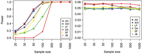
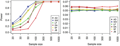
The power of all the tests based on the standard and convoluted non-normal distributions was also compared. In this case, the alternative hypothesis is true, and so each test should reject the null hypothesis at a minimum power of 95%. The results from the uniform-normal distribution are significantly different from those of the standard unform distribution (Figure 1). Thus, in the case of uniform distribution, the power of the normality test is significantly influenced by measurement uncertainty. The power of the tests towards convoluted uniform-normal distribution showed that all the tests performed poorly and none of them attained a power above 6% (Figure 1). Although, all the tests were less powerful towards uniform-normal distribution, the performance of JB test was better compared to other test. In the case of independent uniform distribution, the JB test is less powerful whilst the DA test performed better compared to the other tests.

Figure 1. Power of normality tests against independent uniform (left panel) and convoluted uniform-normal distributions (right panel) with varying sample sizes.

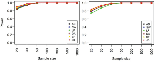
For Student’s t-normal convoluted distribution, the results suggest that the general performance of all the tests is in agreement with that of independent Student’s t distribution (Figure 2). That is, the power of the all the tests increased for an increasing sample size. In addition, all the tests attained their minimum power for a sample size of 50 and above. Thus, the performance of the normality tests remains consistent and better for Student’s t distribution in the presence of measurement uncertainty. Although, all the tests performed better for an increasing sample size, the JB test was consistently the most powerful compared to the other tests followed by the SF test with the LF test being the least powerful. The high performance of the JB test for Student’s t-normal convoluted distribution may be influenced by the fact that the resultant distribution is symmetric with long tails (Thadewald & Büning, 2007). According to Thadewald and Büning (2007,) the JB test is well behaved or has the highest power for symmetric distributions with medium up to long tails.

Figure 2. Power of normality tests against independent Student’s t (left panel) and convoluted Student’s t-normal distributions (right panel) with varying sample sizes.

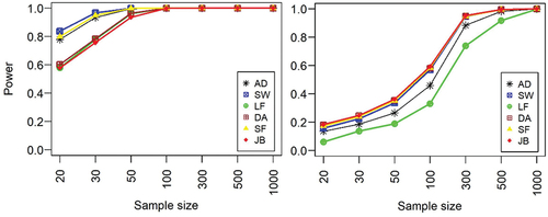
The power of the normality tests for exponential-normal convoluted distribution shows different pattern compared to the results from independent exponential distribution (Figure 3). For exponential-normal convoluted distribution, only SW, AD and JB tests attained a power of 95% at a sample size of 300 whilst the other tests attained the 95% power at sample size of above 300. In the case of standard exponential distribution data, all the tests attained 95% power at sample size of 50 and a maximum power at sample of 100. The power of all the test consistently increases for an increasing sample size for both data. The JB test was consistently the most powerful for exponential-normal distribution data, whilst the SW performs better in the case of standard exponential distribution. The JB test performs poorly in the standard exponential distribution data, whilst the LF test performs poorly in the exponential-normal convoluted distribution data.

Figure 3. Power of normality tests against independent exponential (left panel) and convoluted exponential-normal distributions (right panel) with varying sample sizes.

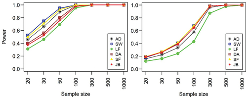
The power of the normality tests towards standard gamma and convoluted gamma-normal distributions increases for an increasing sample size (Figure 4). However, the rate of increment in power for increasing sample size is faster for standard gamma distribution compared to convoluted gamma-normal distribution. For both distributions, the power of SW test outperforms the other tests whilst the LF test consistently remains less powerful. For standard gamma distribution, all the tests attained 95% power for a sample size of 300 except the LF test, whereas in the case of standard gamma distribution, all the tests attained their 95% power for a sample size of 100.

Figure 4. Power of normality tests against independent gamma (left panel) and convoluted gamma-normal distributions (right panel) with varying sample sizes.

Similar to the uniform distribution, the power of all the tests for beta-normal distribution is significantly different from that of the standard beta distribution (Figure 5). That is, for convoluted beta-normal distribution, all the tests perform poorly in terms of power and none of them attained a power of 7% for a sample size of 1000. In the case of standard beta distribution, all the tests attained their full power for a sample of 300. Although all the tests were less powerful towards beta-normal distribution, the performance of JB test was better compared to other test. In the case of standard uniform distribution, the SW test was the most powerful whilst the JB test was the least performed test compared to the other tests.

Figure 5. Power of normality tests against independent beta (left panel) and convoluted beta-normal distributions (right) with varying sample sizes.

4. Conclusions

In this study, the performance of the normality tests (AD, SW, LF, DA, SF and JB tests) towards convoluted distributions was examined based on their Type I error and power. The comparison was done through a Monte Carlo simulation study conducted with different distributions and sample sizes. The results from the simulation experiments revealed that the Type I error rate of the JB test was high compared to the other normality tests considered. None of the tests has a Type I error against the convoluted normal-normal distribution that exceed 6%. The poor performance of the JB test in terms of Type I error is consistent with the finding in the existing literature where independent standard normal distribution was used (Mbah & Paothong, 2015; Yazici & Yolacan, 2007). In addition, the results from the convoluted normal-normal distribution were not different from those of the standard normal distribution. Thus, in the presence of measurement uncertainty which is assumed to be normally distributed, the Type I error rate of all the tests remains unaffected. These results may be influenced by the fact that the resultant distribution under the null hypothesis of all the tests does not change.

The power of all the six normality tests considered was found to be better towards convoluted Student’s t-normal, exponential-normal and gamma-normal distributions for an increasing sample size. However, in the case of convoluted uniform-normal and beta-normal distributions, the power for all the tests remained poor for an increasing sample size. Thus, the presence of measurement uncertainty significantly affects the power of normality tests for uniform and beta distributions. In general, all the normality tests considered were less powerful towards convoluted distribution, particularly for small sample sizes. However, the performance of JB test towards convoluted distributions was found to be better compared to the other tests. For standard distribution, the performance of SW test was found to be better compared to other normality tests considered. The performance of the SW as observed is in agreement with the findings in the existing literature (Adefisoye et al., 2016; Yap & Sim, 2011). Future research will consider using expected p-values computed from the competing tests rather than the power of the tests when the data are assumed to follow a convoluted probability distribution. Such an approach is considered to be optimal than the power of the test which depends on a pre-defined significance level (Mbah & Paothong, 2015; Sackrowitz & Samuel-Cahn, 1999).

Acknowledgements

The authors would like to thank the editor and anonymous reviewers for their comments on earlier drafts of this manuscript.

Disclosure statement

No potential conflict of interest was reported by the author(s).

Additional information

Funding

The authors received no direct funding for this work

Notes on contributors

Desmond Ag-Yi

Desmond Ag-Yi is a graduate of the Department of Statistics and Actuarial Science at Kwame Nkrumah University of Science and Technology, Ghana. His research areas include Statistical Modelling and Simulation.

Eric N. Aidoo

Eric N. Aidoo has a PhD in Statistics from Edith Cowan University, Western Australia. He is currently a Lecturer at the Department of Statistics and Actuarial Science at Kwame Nkrumah University of Science and Technology, Ghana. His research areas include Statistical Modelling, Simulation and Data Analytics.

References

- Adefisoye, J., Golam Kibria, B., & George, F. (2016). Performances of several univariate tests of normality: An empirical study. Journal of Biometrics and Biostatistics, 7 (4) , 1–10 https://doi.org/10.4172/2155-6180.1000322.
- Ahmad, F., & Khan, R. A. (2015). A power comparison of various normality tests. Pakistan Journal of Statistics and Operation Research, 11(3), 331–345. https://doi.org/10.18187/pjsor.v11i3.845
- Anderson, T. W., & Darling, D. A. (1954). A test of goodness of fit. Journal of the American Statistical Association, 49(268), 765–769. https://doi.org/10.1080/01621459.1954.10501232
- Barrera, N. P., Galea, M., Torres, S., & Villalón, M. (2006). Class of skew-distributions: Theory and applications in biology. Statistics, 40(4), 365–375. https://doi.org/10.1080/02331880600741780
- Bono, R., Blanca, M. J., Arnau, J., & Gómez-Benito, J. (2017). Non-normal distributions commonly used in health, education, and social sciences: A systematic review. Frontiers in Psychology, 8, 1–6. https://doi.org/10.3389/fpsyg.2017.01602
- Brandt, S. (1970). Statistical and computational methods in data analysis. Neuropadiatrie, 2(2). https://doi.org/10.1055/s-0028-1091858;https://www.jstor.org/stable/2335012
- D’Agostino, R. B. (1971). An omnibus test of normality for moderate and large size samples. Biometrika, 58(2), 341–348. https://doi.org/10.1093/biomet/58.2.341
- D’Agostino, R., & Pearson, E. S. (1973). Tests for departure from normality. Empirical results for the distributions of b2 and √b1. Biometrika, 60(3) , 613–622 https://doi.org/10.2307/2335012.
- Dominguez, A. (2015). A history of the convolution operation [Retrospectroscope]. IEEE Pulse, 6(1), 38–49. https://doi.org/10.1109/MPUL.2014.2366903
- Gel, Y. R., & Gastwirth, J. L. (2008). A robust modification of the Jarque–Bera test of normality. Economics Letters, 99(1), 30–32. https://doi.org/10.1016/j.econlet.2007.05.022
- Grinstead, C. M., & Snell, J. L. (2012). Introduction to probability. American Mathematical Soc.
- Hain, J. (2010). Comparison of common tests for normality. Diploma Thesis, Julius-Maximilians-Universität of Würzburg.
- Jarque, C. M., & Bera, A. K. (1987). A test for normality of observations and regression residuals. International Statistical Review/Revue Internationale de Statistique 55(2) , 163–172 https://doi.org/10.2307/1403192.
- Kang, J. S., Kim, S. L., Kim, Y. H., & Jang, Y. S. (2010). Generalized convolution of uniform distributions. Journal of Applied Mathematics & Informatics, 28(5–6) , 1573–1581 https://koreascience.kr/article/JAKO201008758942063.pdf.
- King, G., Tomz, M., & Wittenberg, J. (2000). Making the most of statistical analyses: Improving interpretation and presentation. American Journal of Political Science, 44(2), 347–361. https://doi.org/10.2307/2669316
- Lilliefors, H. W. (1967). On the Kolmogorov-Smirnov test for normality with mean and variance unknown. Journal of the American Statistical Association, 62(318), 399–402. https://doi.org/10.1080/01621459.1967.10482916
- Lumley, T., Diehr, P., Emerson, S., & Chen, L. (2002). The importance of the normality assumption in large public health data sets. Annual Review of Public Health, 23(1), 151–169. https://doi.org/10.1146/annurev.publhealth.23.100901.140546
- Maas, C. J., & Hox, J. J. (2004). The influence of violations of assumptions on multilevel parameter estimates and their standard errors. Computational Statistics & Data Analysis, 46(3), 427–440. https://doi.org/10.1016/j.csda.2003.08.006
- Mbah, A. K., & Paothong, A. (2015). Shapiro–Francia test compared to other normality test using expected p -value. Journal of Statistical Computation and Simulation, 85(15), 3002–3016. https://doi.org/10.1080/00949655.2014.947986
- Monhor, D. (2005). On the relevance of convolution of uniform distributions to the theory of errors. Acta Geodaetica et Geophysica Hungarica, 40(1), 59–68. https://doi.org/10.1556/AGeod.40.2005.1.5
- Noughabi, H. A., & Arghami, N. R. (2011). Monte Carlo comparison of seven normality tests. Journal of Statistical Computation and Simulation, 81(8), 965–972. https://doi.org/10.1080/00949650903580047
- Pogány, T. K., & Nadarajah, S. (2013). On the convolution of normal and t random variables. Statistics, 47(6), 1363–1369. https://doi.org/10.1080/02331888.2012.694447
- R Core Team (2020). R: A language and environment for statistical computing. R Foundation for Statistical Computing. https://www.R-project.org/
- Sackrowitz, H., & Samuel-Cahn, E. (1999). P values as random variables—expected P values. The American Statistician, 53(4) , 326–331 https://doi.org/10.2307/2686051.
- Shapiro, S. S., & Wilk, M. B. (1965). An analysis of variance test for normality (complete samples). Biometrika, 52(3–4), 591–611. https://doi.org/10.1093/biomet/52.3–4.591
- Shapiro, S. S., & Francia, R. (1972). An approximate analysis of variance test for normality. Journal of the American Statistical Association, 67(337), 215–216. https://doi.org/10.1080/01621459.1972.10481232
- Sitek, G. (2020). Sum of gamma and normal distribution. Zeszyty Naukowe. Organizacja i Zarządzanie/Politechnika Śląska, (143), 275–284 https://doi.org/10.29119/1641-3466.2020.143.22 .
- Thadewald, T., & Büning, H. (2007). Jarque–Bera test and its competitors for testing normality–a power comparison. Journal of Applied Statistics, 34(1), 87–105. https://doi.org/10.1080/02664760600994539
- Wijekularathna, D. K., Manage, A. B. W., & Scariano, S. M. (2022). Power analysis of several normality tests: A Monte Carlo simulation study. Communications in Statistics - Simulation and Computation, 51(3), 757–773. https://doi.org/10.1080/03610918.2019.1658780
- Yap, B. W., & Sim, C. H. (2011). Comparisons of various types of normality tests. Journal of Statistical Computation and Simulation, 81(12), 2141–2155. https://doi.org/10.1080/00949655.2010.520163
- Yazici, B., & Yolacan, S. (2007). A comparison of various tests of normality. Journal of Statistical Computation and Simulation, 77(2), 175–183. https://doi.org/10.1080/10629360600678310
- Zamanzade, E., & Arghami, N. R. (2011). Goodness-of-fit test based on correcting moments of modified entropy estimator. Journal of Statistical Computation and Simulation, 81(12), 2077–2093. https://doi.org/10.1080/00949655.2010.517533
- Zamanzade, E., & Arghami, N. R. (2012). Testing normality based on new entropy estimators. Journal of Statistical Computation and Simulation, 82(11), 1701–1713. https://doi.org/10.1080/00949655.2011.592984
- Zamanzade, E., & Mahdizadeh, M. (2017). Entropy estimation from ranked set samples with application to test of fit. Revista Colombiana de Estadística, 40(2), 223–241. https://doi.org/10.15446/rce.v40n2.58944