Singularly perturbed reaction diffusion problem with large spatial delay via non-standard fitted operator method

ABSTRACT

In this article, a numerical method for singularly perturbed partial differential equations of the reaction-diffusion type with a large spatial delay is constructed. The method is developed using the Crank-Nicolson method for time derivative and a non-standard finite difference method for spatial derivative on a uniform mesh. Due to the presence of a small perturbation parameter, which multiplies the highest order derivative term, the solution exhibits twin boundary layers. The solution to the problem also shows an interior layer as a result of the delay in the spatial variable. To enhance the order of convergence, the Richardson extrapolation technique is applied. The convergence analysis of the proposed scheme is given. It is proved that the resulting scheme is uniformly convergent of fourth-order accurate in both space and time variables. Numerical experiments are conducted, and the results are in agreement with the theoretical findings. In addition, comparisons are performed, and the results show that the proposed scheme gives more accurate solutions and a higher rate of convergence than previous findings in the literature.

KEYWORDS:

• Singular perturbation
• reaction diffusion problem
• nonstandard finite difference
• large space delay
• Crank-Nicolson

1 Introduction

Singularly perturbed reaction-diffusion with delay in the spatial variable arise especially in the theoretical analysis of neuronal variability, for example in determination of the behavior of a neuron to random synaptic inputs (Brdar et al., 2023; Kumar & Kumari, 2020; Stein, 1965, 1967). The first paper on this area was given in Stein (1965), where he proposed a practical model for the stochastic effects due to the neuronal variability and obtained the approximate solution to the differential difference equation model using Monte Carlo techniques. In Musila & Petr (1991), the authors generalized Stein’s model and proposed a mathematical model in terms of singularly perturbed parabolic partial differential-difference equations to consider the time evolution trajectories of the membrane potential.

Lange and Miura were the first to consider various classes of singularly perturbed ordinary differential equations with small shifts appearing in the solution and its first derivative, and they used an asymptotic approach for analysis (Lange & Miura, 1994).

Dealing with the approximate solution of a time-dependent singularly perturbed parabolic problem (SPPP) that contains a shift argument is not a simple task in contrast to problems not having a shift argument. Numerous authors have developed a number of numerical methods for the solution of SPPPs with a large or small delay in the temporal direction, to name a few (Ayele, Tiruneh, Derese et al., 2022; Babu & Bansal, 2022; Burcu, 2021; Kumar, 2021; Kumar et al., 2019; Kumar & Kumari, 2019; Negero & Duressa, 2022) and authors in Ayele, Tiruneh, Derese et al., 2022; Bansal et al., 2017; Bansal & Sharma, 2017; Choudhary & Kaushik, 2022; Daba & Duressa, 2021; Duressa & Woldaregay, 2022; Kaushik & Sharma, 2020; Kumar & Kadalbajoo, 2011; Prathap & Nageshwar Rao, 2022; Ramesh & Kadalbajoo, 2008; Woldaregay et al., 2021, have also recently achieved advancements in numerical methods for the solution of SPPP of the convection diffusion type with a delay on the spatial variable.

However, SPPP of reaction diffusion type with shift in the spatial variable is less investigated as compared to convection diffusion type problems. As far as our knowledge goes, few studies have been conducted on these problems. The authors in Kumar & Kumari (2020); Parthiban et al. (2015) considered SPPP of reaction diffusion type with a large delay in the spatial direction, the Crank-Nicolson scheme on a uniform mesh for the discretization of the time variable, and the standard finite difference scheme on a piecewise-uniform mesh for the discretization of spatial variable is applied. Furthermore, the author in Bansal & Sharma (2018) made use of the implicit Euler method on a uniform mesh, and the finite difference method on piecewise uniform meshes to discretize the temporal and spatial variables, respectively, for the problem discussed in Kumar & Kumari (2020).

In Elango et al. (2021), singularly perturbed delay differential equations (SPDDE) of the reaction diffusion type with integral boundary conditions are studied via the backward Euler scheme for the temporal direction and a standard finite difference scheme on a piecewise uniform mesh (Shishkin mesh) for the spatial discretization.

In Gobena et al. (2021), the authors designed a fitted operator scheme using a nonstandard finite difference scheme on a uniform mesh for the spatial variable discretization and the backward Euler scheme for the temporal variable discretization, for the problem in Elango et al. (2021). The problem that is discussed in Elango et al. (2021); Gobena et al. (2021) is also investigated in Hailu et al. (2022), the scheme is formulated by combining the cubic spline method in the spatial direction on a piecewise uniform mesh and the implicit Euler method in the temporal direction on uniform meshes.

In Gelu et al. (2021), SPDDE of a reaction-diffusion type with mixed-type boundary conditions is considered. The implicit Euler method on a uniform mesh for the discretization of the time derivative and the extended cubic B-spline collocation method on a Shishkin mesh for the space variable discretization is applied. Also, the SPPP of a reaction diffusion type with a large spatial delay is considered in Ejere et al. (2022). The scheme is developed by employing the central difference technique on a piecewise uniform mesh in the space direction and the weighted average ($\theta$-method) on a uniform mesh, and it is proved that the resulting scheme is an almost second-order convergent.

The authors in Brdar et al. (2023), discussed the solution of SPPP of reaction diffusion type with a large delay in the spatial direction; the standard finite element method on two different classes of layer-adapted meshes for the discretization of the space variable is used, and for the time discretization, the discontinuous Galerkin (dG) method is applied.

Inspired by the study of Brdar et al. (2023), we constructed a uniformly convergent method for SPPP of reaction diffusion type with a large shift in the spatial variable. The approach is developed using the Crank-Nicolson method for time derivatives on a uniform mesh, and in the spatial direction, a non-standard finite difference method on a uniform mesh is applied. The Richardson extrapolation technique is used in order to enhance accuracy and order of convergence. The advantages of the proposed scheme are that it is a uniformly convergent scheme without any restrictions on the number of mesh intervals, it has high accuracy and high rate of convergence, and the approach used in the scheme formulation is also easily adaptable to small delays.

Notation: $C$ and its subscripts denote positive constants independent of $\epsilon$ and mesh sizes. Also $||.||$ denotes the standard supremum norm, defined as $\mathrm{\setminus }\mathrm{b}\mathrm{r}\mathrm{e}\mathrm{a}\mathrm{k}\left|\left|f\right|\right|=\underset{\left(x,t\right)\in \bar{D}}{Sup}\left|f\left(x,t\right)\right|,$ for a function $f$ defined on domain $\bar{D}$.

2 Problem formulation

Consider the following time-dependent SPP of reaction diffusion type with large spatial delay:

(2.1) $\frac{\mathrm{\partial }u}{\mathrm{\partial }t}-{\epsilon }^2\frac{{\mathrm{\partial }}^{2}u}{\mathrm{\partial }{x}^2}+\beta (x)u(x,t)+\gamma (x)u(x-1,t)=f(x,t),(x,t)\in D,$(2.1)

subject to the following initial condition and interval boundary conditions,

(2.2) $\begin{array}{cc}\hspace{0.17em}& u\left(x,0\right)={\phi }_0\left(x\right),\left(x,0\right)\in {\mathrm{\Gamma }}_0=\left\{\left(x,t\right):0\le x\le 2\mathrm{a}\mathrm{n}\mathrm{d}t=0\right\},\\ \hspace{0.17em}& u\left(x,t\right)={\phi }_l\left(x,t\right),\left(x,t\right)\in {\mathrm{\Gamma }}_l=\left\{\left(x,t\right):\left(x,t\right)\in \left[-1,0\right]\times \mathrm{\Lambda }\right\},\\ \hspace{0.17em}& u\left(2,t\right)={\phi }_r\left(t\right),\left(2,t\right)\in {\mathrm{\Gamma }}_r=\left\{\left(2,t\right):t\in \bar{\mathrm{\Lambda }}\right\},\end{array}$(2.2)

where $0<\epsilon <<1$ is the perturbation parameter, $D=\mathrm{\Omega }\times \mathrm{\Lambda }$, $D_l=(0,1)\times \mathrm{\Lambda }$, $D_r=(1,2)\times \mathrm{\Lambda }$, $\mathrm{\Omega }=(0,2)$, and $\mathrm{\Lambda }=(0,1]$. The function $\beta (x),\gamma (x),{\phi }_0(x),{\phi }_l(x,t),{\phi }_r(t)$, and $f(x,t)$ are sufficiently smooth, bounded and independent of $\epsilon$, $\mathrm{\forall }(x,t)\in \bar{D}$. Moreover, assume that $\beta (x)$ and $\gamma (x)$ satisfy

(2.3) $\beta (x)\ge {\beta }_0>0,\gamma (x)<0\mathrm{a}\mathrm{n}\mathrm{d}\beta (x)+\gamma (x)>0,x\in \bar{\mathrm{\Omega }}.$(2.3)

where ${\beta }_0$ are constant. The solution of (2.1) satisfies $[u]=u(1^{+},t)-u(1^{-},t)=0$ and $[u_x]=\frac{\mathrm{\partial }}{\mathrm{\partial }x}(1^{+},t)-\frac{\mathrm{\partial }}{\mathrm{\partial }x}(1^{-},t)=0$ at $x=1$, here $u(1^{-},t)$ and $u(1^{+},t)$ are left- and right-side limit of $u$ at $x=1.$

The problem defined in (2.1) can be rewritten as

(2.4) ${\mathcal{L}}_{\epsilon }u(x,t)=g(x,t),$(2.4)

where

(2.5) ${\mathcal{L}}_{\epsilon }u(x,t)\equiv \left\{\begin{array}{c}\frac{\mathrm{\partial }u}{\mathrm{\partial }t}-{\epsilon }^2\frac{{\mathrm{\partial }}^{2}u}{\mathrm{\partial }{x}^2}+\beta (x)u(x,t),\mathrm{f}\mathrm{o}\mathrm{r}(x,t)\in (0,1]\times \mathrm{\Lambda },\\ \frac{\mathrm{\partial }u}{\mathrm{\partial }t}-{\epsilon }^2\frac{{\mathrm{\partial }}^{2}u}{\mathrm{\partial }{x}^2}+\beta (x)u(x,t)\\ +\gamma (x)u(x-1,t),\mathrm{f}\mathrm{o}\mathrm{r}(x,t)\in (1,2)\times \mathrm{\Lambda },\end{array}\right.$(2.5)

and

(2.6) $g(x,t)=\left(\begin{array}{c}f(x,t)-\gamma (x)\phi (x-1,t),\mathrm{f}\mathrm{o}\mathrm{r}(x,t)\in (0,1]\times \mathrm{\Lambda },\\ f(x,t),\mathrm{f}\mathrm{o}\mathrm{r}(x,t)\in (1,2)\times \mathrm{\Lambda },\end{array}\right.$(2.6)

with the given initial and boundary condition. The solution $u(x,t)$ of problem (2.1) exhibits strong interior layer at $x=1$ and parabolic boundary layers in the neighborhood ${\mathrm{\Gamma }}_l$ and ${\mathrm{\Gamma }}_r$. The boundary layer is parabolic because of the reduced problem $(\epsilon =0)$ of the (2.1) are parallel to the boundary of the domain.

3 Some analytical results

In this section, the analytical aspects of the solution of problem (2.1) and its derivatives are studied. The existence and uniqueness of the solution of problem (2.1) can be established under the assumption that the data are Hölder continuous and also satisfying the following compatibility conditions:

${\phi }_0(0)={\phi }_l(0,0),{\phi }_0(2)={\phi }_r(0),$

$\frac{\mathrm{\partial }{\phi }_l(0,0)}{\mathrm{\partial }t}-{\epsilon }^2\frac{{\mathrm{\partial }}^2{\phi }_0(0)}{\mathrm{\partial }{x}^2}+\beta (0){\phi }_0(0)+\gamma (0){\phi }_l(-1,0)=f(0,0),$

$\frac{\mathrm{\partial }{\phi }_r(0)}{\mathrm{\partial }t}-{\epsilon }^2\frac{{\mathrm{\partial }}^2{\phi }_0(2)}{\mathrm{\partial }{x}^2}+\beta (2){\phi }_0(2)+\gamma (2){\phi }_r(1,0)=f(2,0).$

The problem (2.1) has a unique solution with the above conditions and assumptions (Bansal & Sharma, 2018; Ladyzhenskaia et al., 1988; Parthiban et al., 2015).

Lemma 3.1 (Maximum principle). Suppose $\zeta (x,t)\in C^{(0,0)}(\bar{D})\cap C^{(1,0)}(D)\cap C^{(2,1)}(D_l\cup D_r)$.If $\zeta (x,t)\ge 0$, $\mathrm{\forall }(x,t)\in \mathrm{\partial }D$,and ${\mathcal{L}}_{\epsilon }\zeta (x,t)\ge 0,\mathrm{\forall }(x,t)\in (D_l\cup D_r)$ and $[{\zeta }_x](1,t)={\zeta }_x(1^{+},t)-{\zeta }_x(1^{-},t)\le 0$. Then $\zeta (x,t)\ge 0,\mathrm{\forall }(x,t)\in \bar{D}$.

Proof. Define a test function

(3.1) $\nu (x,t)=\left\{\begin{array}{c}\frac{3}{2}+\frac{x}{2},(x,t)\in {\bar{D}}_l,\\ 3-x,(x,t)\in {\bar{D}}_r.\end{array}\right.$(3.1)

Note that $\nu (x,t)>0,\mathrm{\forall }(x,t)\in \bar{D},{\mathcal{L}}_{\epsilon }\nu (x,t)>0,\mathrm{\forall }\text{break}(x,t)\in (D_l\cup D_r)$ and $[{\nu }_x](1,t)<0.$ Assume

$\eta =\mathrm{m}\mathrm{a}\mathrm{x}\{\frac{-\zeta (x,t)}{\nu (x,t)}:(x,t)\in \bar{D}\}.$

Then there exists $(x^o,t^o)\in \bar{D}$ such that $\zeta (x^o,t^o)+\eta \nu (x^o,t^o)=0$ and $\zeta (x,t)+\eta \nu (x,t)\ge 0$, $\mathrm{\forall }(x,t)\in \bar{D}.$ Therefore, the function attains minimum at $(x^o,t^o).$ Suppose the theorem doesn’t hold true, then $\eta >0$

Case 1: $(x^o,t^o)\in D_l$,

(3.2) $0\le {\mathcal{L}}_{\epsilon }\zeta (x^o,t^o)=\frac{\mathrm{\partial }\zeta }{\mathrm{\partial }t}(x^o,t^o)-{\epsilon }^2\frac{{\mathrm{\partial }}^2\zeta }{\mathrm{\partial }{x}^2}(x^o,t^o)+\beta (x^o)\zeta (x^o,t^o)<0,$(3.2)

Case 2: $(x^o,t^o)=(1,t^o)$,

$0\le [(\zeta +\eta \nu {)}_x](x^o,t^o)=[{\zeta }_x](x^o,t^o)+\eta [{\nu }_x](x^o,t^o)<0,$

Case 3: $(x^o,t^o)\in D_r$,

(3.3) $\begin{array}{cc}0\le {\mathcal{L}}_{\epsilon }\zeta \left(x^o,t^o\right)& =\frac{\mathrm{\partial }\zeta }{\mathrm{\partial }t}\left(x^o,t^o\right)-{\epsilon }^2\frac{{\mathrm{\partial }}^2\zeta }{\mathrm{\partial }{x}^2}\left(x^o,t^o\right)\\ \hspace{0.17em}& +\beta \left(x^o\right)\zeta \left(x^o,t^o\right)+\gamma \left(x^o\right)\zeta \left(x^o-1,t^o\right)\\ \hspace{0.17em}& =\frac{\mathrm{\partial }\zeta }{\mathrm{\partial }t}\left(x^o,t^o\right)-{\epsilon }^2\frac{{\mathrm{\partial }}^2\zeta }{\mathrm{\partial }{x}^2}\left(x^o,t^o\right)\\ \hspace{0.17em}& +\left(\beta \left(x^o\right)+\gamma \left(x^o\right)\right)\zeta \left(x^o,t^o\right)\\ \hspace{0.17em}& -\gamma \left(x^o\right)\left(\zeta \left(x^o,t^o\right)-\zeta \left(x^o-1,t^o\right)\right)<0.\end{array}$(3.3)

In all cases it is a contradiction. Hence, $\zeta (x,t)\ge 0,\mathrm{\forall }(x,t)\in \bar{D}$.

The next lemma demonstrates the stability of the operator ${\mathcal{L}}_{\epsilon }$ and the $\epsilon -$ uniform boundedness for the solution of (2.1) in the maximum norm.

Lemma 3.2. The solution $u(x,t)$ of problem (2.1) is bounded and satisfies the following estimate:

(3.4) $||u(x,t)|{|}_{\bar{D}}\le Cmax\{||{\mathcal{L}}_{\epsilon }u|{|}_D,||{\phi }_0(x)||,||{\phi }_l(x,t)||,||{\phi }_r(t)||\},\mathrm{\forall }(x,t)\in \bar{D}.$(3.4)

Proof. Consider a barrier function $\mathrm{\Phi }\underset{\_}{+}(x,t)=CK\nu (x,t)\underset{\_}{\text{break}}+u(x,t),(x,t)\in \bar{D}$, where $K=\mathrm{m}\mathrm{a}\mathrm{x}\{||{\mathcal{L}}_{\epsilon }u|{|}_D,||{\phi }_0(x)||,\text{break}||{\phi }_l(x,t)||,||{\phi }_r(t)||\}$ and $\nu (x,t)$ is test function. Then by taking the barrier function and Lemma 3.1,it can be easily proved. □

Lemma 3.3. The solution of the problem (2.1) satisfies the following bound:

$|u(x,t)-{\phi }_0(x)|\le Ct,(x,t)\in D.$

Proof. Please follow procedure in Roos et al. (2008).

Lemma 3.4. The solution $u(x,t)$ of (2.1) satisfies the bound

$|u(x,t)|\le C,\mathrm{\forall }(x,t)\in \bar{D}.$

Proof. Taking $|u(x,t)|=|u(x,t)-{\phi }_0(x)+{\phi }_0(t)|\le |u(x,t)-{\phi }_0(t)|+|{\phi }_0(t)|.$ Using Lemma (3.3), $|u(x,t)|\le Ct+|{\phi }_0(x)|$, and we have ${\phi }_0(x)$ is bounded and $t\in (0,T]$. Hence, we get the required result.

Lemma 3.5. Under the hypothesis of Lemma 3.3 and 3.4, the derivative of $u(x,t)$ satisfies the following bound:

$|u_t(x,t)|\le C,(x,t)\in \bar{D}.$

Proof. Please see Bansal & Sharma (2018). □

4 Description of the numerical scheme

To obtain the discrete scheme, we discretized the temporal variable and space variable separately as follows:

4.1 Temporal semi-discretization

On the time domain $[0,T]$, we use uniform mesh given by: ${\mathrm{\Lambda }}^M=\{t_j:t_j=j\mathrm{\Delta }t,\mathrm{\Delta }t=\frac{T}{M},\mathrm{f}\mathrm{o}\mathrm{r}j=0,1,\dots ,M\}$, where $M$ is the number of mesh intervals in $[0,T]$ and $\mathrm{\Delta }t$ is the time step. To approximate the temporal derivative term of (2.1) on ${\mathrm{\Lambda }}^M$, we use Crank Nicolson method as follows:

(4.1) $\frac{u^{j+1}-u^j}{\mathrm{\Delta }t}-{\epsilon }^2\frac{{\mathrm{\partial }}^2}{\mathrm{\partial }{x}^2}u(x,t_{j+1/2})+\beta (x)u(x,t_{j+1/2})+\gamma (x)u(x-1,t_{j+1/2})=f(x,t_{j+1/2}).$(4.1)

Subject to the following initial and interval boundary condition(IIBC):

(4.2) $\begin{array}{rl}& u(x,0)={\phi }_0(x),(x,0)\in {\mathrm{\Gamma }}_0\\ & =\{(x,t):0\le x\le 2\mathrm{a}\mathrm{n}\mathrm{d}t=0\},\\ & u(x,t_{j+1})={\phi }_l(x,t_{j+1}),(x,t_{j+1})\in {\mathrm{\Gamma }}_l^M\\ & =\{(x,t_{j+1}):-\delta \le x\le 0,0\le j\le M-1\},\\ & u(2,t_{j+1})={\phi }_r(t_{j+1}),(2,t_{j+1})\in {\mathrm{\Gamma }}_r^M\\ & =\{(2,t_{j+1}):0\le j\le M-1\},\end{array}$(4.2)

where

$u(x,t_{j+1/2})=\frac{u(x,t_{j+1})+u(x,t_j)}{2},f(x,t_{j+1/2})=\frac{f(x,t_{j+1})+f(x,t_j)}{2}.$

After some rearrangement the temporal semi-discretized form of (2.1) is given by

(4.3) ${\mathcal{L}}_{\epsilon }^{M}u(x,t_{j+1})=G(x,t_j),$(4.3)

where

(4.4) ${\mathcal{L}}_{\epsilon }^{M}u(x,t_{j+1})=\left\{\begin{array}{c}-{\epsilon }^2\frac{{\mathrm{\partial }}^2}{\mathrm{\partial }{x}^2}{u}^{j+1}+(\beta (x)+2/\mathrm{\Delta }t)u^{j+1},\mathrm{f}\mathrm{o}\mathrm{r}x\in (0,1],\\ -{\epsilon }^2\frac{{\mathrm{\partial }}^2}{\mathrm{\partial }{x}^2}{u}^{j+1}+(\beta (x)+2/\mathrm{\Delta }t)u^{j+1}\\ +\gamma (x,t)u(x-1,t_{j+1}),\mathrm{f}\mathrm{o}\mathrm{r}x\in (0,2),\end{array}\right.$(4.4)

where

$G(x,t_j)=\left\{\begin{array}{c}{\epsilon }^2\frac{{\mathrm{\partial }}^2}{\mathrm{\partial }{x}^2}{u}^j-(\beta (x)-2/\mathrm{\Delta }t)u^j\\ +2\gamma (x)u(x-1,t_{j+1/2})+2f(x,t_{j+1/2}),x\in (0,1],\\ {\epsilon }^2\frac{{\mathrm{\partial }}^2}{\mathrm{\partial }{x}^2}{u}^j-(\beta (x)-2/\mathrm{\Delta }t)u^j\\ +\gamma (x,t)u(x-1,t_j)+2f(x,t_{j+1/2}),x\in (1,2),\end{array}\right.$

and, $u^{j+1}(x)$ and $u_{j+1}(x)$ are the semi-discrete approximation to the exact solution $u(x,t)$ of (2.1) at the $(j+1{)}^{th}$ time level. The local truncation error of the semi-discrete method (4.3) is given by

$e_{j+1}^{\ast }=u(x,t_{j+1})-u_{j+1}(x).$

Lemma 4.1. Suppose $\zeta (x,t_{j+1})$ be a smooth function $\mathrm{\forall }x\in \bar{\mathrm{\Omega }}$. If $\zeta (0,t_{j+1})\ge 0,\zeta (2,t_{j+1})\ge 0$, ${\mathcal{L}}_{\epsilon }^M\zeta (x,t_{j+1})\ge 0,\mathrm{\forall }x\in \mathrm{\Omega }\mathrm{\setminus }\{1\}$ and $[{\zeta }_x](1,t_{j+1})={\zeta }_x(1^{+},t_{j+1})-{\zeta }_x(1^{-}\text{break},t_{j+1})\le 0$,then $\zeta (x,t_{j+1})\ge 0,\mathrm{\forall }x\in \bar{\mathrm{\Omega }}$.

Proof. Follow the same procedure as Lemma 3.1. □

Lemma 4.2. If $u(x,t_{j+1})$ satisfies problem (4.3),then the bound

(4.5) $|u(x,t_{j+1})||\le Cmax\{||{\mathcal{L}}_{\epsilon }^M{u}_{j+1}(x)||,||{\phi }_l(x,t_{j+1})||,\text{break}||{\phi }_r(t_{j+1})||,||{\phi }_0(x)||\},\mathrm{\forall }x\in [0,2].$(4.5)

Proof. Take the following barrier function: ${\mathrm{\Phi }}^{\underset{\_}{+}}(x,t_{j+1})=C\tilde{K}\nu (x,t_{j+1})\underset{\_}{+}u(x,t_{j+1}),x\in [0,2]$, where $\tilde{K}=\mathrm{m}\mathrm{a}\mathrm{x}\{||{\mathcal{L}}_{\epsilon }^{M}u(x,t_{j+1})||,||{\phi }_l(x,t_{j+1})||,||{\phi }_r(t_{j+1})||,\text{break}||{\phi }_0(t_{j+1})||\}$, and $\nu (x,t_{j+1})$ is test function. It is can be proved using barrier function and Lemma 3.1. □

Lemma 4.3. Suppose that $\left|\frac{{\mathrm{\partial }}^v}{\mathrm{\partial }{t}^v}u(x,t)\right|\le C,(x,t)\text{break}\in \bar{\mathrm{\Omega }},v=0,1,2,3$, the local truncation error associated to scheme (4.3) satisfies:

(4.6) $||e_{j+1}^{\ast }|{|}_{\mathrm{\infty }}\le C_1(\mathrm{\Delta }t{)}^3,j=0,1,2,\dots ,M-1.$(4.6)

Proof. Using Taylor’s series expansion, expand $u(x,t_{j+1})$ and $u(x,t_j)$ centered at $t_{j+1/2}$,we get

(4.7) $\frac{u(x,t_{j+1})-u(x,t_j)}{\mathrm{\Delta }t}=u_t(x,t_{j+1/2})+O((\mathrm{\Delta }t{)}^2),$(4.7)

Then substitute (4.7) into (2.1), we can get

(4.8) $\begin{array}{rl}& \frac{u(x,t_{j+1})-u(x,t_j)}{\mathrm{\Delta }t}={\epsilon }^2\frac{d}{d{x}^2}u(x,t_{j+1/2})\\ & -\beta (x)u(x,t_{j+1/2})-\gamma (x)u(x-1,t_{j+1/2})\\ & +f(x,t_{j+1/2})+O((\mathrm{\Delta }t{)}^2),\end{array}$(4.8)

where

$f(x,t_{j+1/2})=\frac{f(x,t_{j+1})+f(x,t_j)}{2}+O((\mathrm{\Delta }t{)}^2),$

$u(x,t_{j+1/2})=\frac{u(x,t_{j+1})+u(x,t_j)}{2}+O((\mathrm{\Delta }t{)}^2).$

Now, from (4.8), the local truncation error $||e_{j+1}^{\ast }||$ is the solution of the following problem:

(4.9) $\left\{\begin{array}{c}{\mathcal{L}}_{\epsilon }^M{e}_{j+1}^{\ast }=O((\mathrm{\Delta }t{)}^3),\\ e_{j+1}^{\ast }(0)=0,e_{j+1}^{\ast }(2)=0.\end{array}\right.$(4.9)

Then, using the maximum principle for the operator ${\mathcal{L}}_{\epsilon }^M$ proves the result.

Theorem 4.1 (Global error estimate). Under the hypothesis of Lemma 4.3, the global error estimate $E_{j+1}^{\ast }=u(x,t_{j+1})-u^{j+1}(x)={\sum }_{k=1}^j{e}_k^{\ast }$, associated with Crank-Nicolson scheme in the time direction at $(j+1{)}^{th}$ time level is given by:

$||E_{j+1}^{\ast }|{|}_{\mathrm{\infty }}\le C(\mathrm{\Delta }t{)}^2,forj=0,1,2,\dots ,M-1.$

Proof. Utilize the local error estimate in Lemma 4.3 to derive the global error estimates at the $(z+1{)}^{th}$ time level as follows:

(4.10) $\begin{array}{cc}||E_{z+1}^{\ast }||& =||\sum _{\rho =1}^z{e}_{\rho }^{\ast }||,z\le T/\mathrm{\Delta }t\\ \hspace{0.17em}& \le ||e_1^{\ast }||+||e_2^{\ast }||+\dots +||e_z^{\ast }||\\ \hspace{0.17em}& \le C_{1}z{(\mathrm{\Delta }t)}^3,\mathrm{b}\mathrm{y}Lemma4.3\\ \hspace{0.17em}& \le C_1(z\mathrm{\Delta }t)(\mathrm{\Delta }t{)}^2,\\ \hspace{0.17em}& \le C_{1}T{(\mathrm{\Delta }t)}^2,\mathrm{s}\mathrm{i}\mathrm{n}\mathrm{c}\mathrm{e}z\mathrm{\Delta }t\le T\\ \hspace{0.17em}& \le C{(\mathrm{\Delta }t)}^2,C_{1}T=C.\end{array}$(4.10)

Lemma 4.4. The derivatives of the solution $u(x,t_{j+1})$ of the semi-discretized problem (4.3) satisfies the following bound,for $n=0,1,2,3,4.$

(4.11) $\left|\frac{d^{n}u(x,t_{j+1})}{d{x}^n}\right|\le C\left\{\begin{array}{c}1+{\epsilon }^{-n}\left[\mathrm{e}\mathrm{x}\mathrm{p}(-x\frac{\sqrt{{\beta }_0}}{\epsilon })+\mathrm{e}\mathrm{x}\mathrm{p}(-(1-x)\frac{\sqrt{{\beta }_0}}{\epsilon })\right],x\in [0,1],\\ 1+{\epsilon }^{-n}\left[\mathrm{e}\mathrm{x}\mathrm{p}(-(x-1)\frac{\sqrt{{\beta }_0}}{\epsilon })+\mathrm{e}\mathrm{x}\mathrm{p}(-(2-x)\frac{\sqrt{{\beta }_0}}{\epsilon })\right],x\in [1,2].\end{array}\right.$(4.11)

Proof. Please refer (Bansal & Sharma, 2018; Clavero & Gracia, 2010; Manikandan et al., 2014).

4.2 Spatial discretization

The domain of the spatial variable $\bar{\mathrm{\Omega }}$ is discretized uniformly as follows:

${\bar{\mathrm{\Omega }}}^N=\{0=x_0,x_1,\dots ,x_N=2\},x_i=x_0+ih,h=\frac{2}{N},\mathrm{f}\mathrm{o}\mathrm{r}i=1,2,..,N-1,$

where $N$ is the number of mesh intervals in the spatial direction. Thus, the domain of problem (2.1) is discretized as ${\bar{D}}^{N,M}={\bar{\mathrm{\Omega }}}^N\times {\mathrm{\Lambda }}^M$. In addition, the following are some discretized subdomains used in the next section. $D_l^{\ast N,M}=\{x_1,x_2,\dots ,x_{\frac{N}{2}-1},x_{\frac{N}{2}}\}\times {\mathrm{\Lambda }}^M$, $D_l^{N,M}=\{x_1,\dots ,x_{\frac{N}{2}-1}\}\times {\mathrm{\Lambda }}^M$ and $D_r^{N,M}=\{x_{\frac{N}{2}+1},x_{\frac{N}{2}\text{break}+2}\dots ,x_{N-1}\}\times {\mathrm{\Lambda }}^M$. The non-standard finite difference method is further applied to the problem (4.3) in the subsequent sections.

4.2.1 Non-standard finite difference

The core concept of the non-standard finite difference method is to replace the denominator of the finite difference approximation of the derivatives by positive functions. For the construction of an exact finite difference scheme, consider the following constant coefficient homogeneous differential equation, corresponding to (4.3):

(4.12) $-{\epsilon }^2\frac{d}{d{x}^2}{u}^{j+1}+{\beta }^{\ast }{u}^{j+1}=0,$(4.12)

where $(\beta (x)+2/\mathrm{\Delta }t)>{\beta }^{\ast }.$ Then, from (4.12) we have two linearly independent solution, given as:

(4.13) $\mathrm{e}\mathrm{x}\mathrm{p}({\theta }_{1}x)\mathrm{a}\mathrm{n}\mathrm{d}\mathrm{e}\mathrm{x}\mathrm{p}({\theta }_{2}x),{\theta }_{1,2}=\underset{\_}{+}\sqrt{\frac{{\beta }^{\ast }}{{\epsilon }^2}},$(4.13)

where ${\theta }_{1,2}$ are the roots of its corresponding characteristic equation. Then, find a difference equation which has the same general solution as the differential equations in (4.3) at the mesh point $x_i$ given by $U_{i,j+1}=c_1\mathrm{e}\mathrm{x}\mathrm{p}({\theta }_1{x}_i)+c_2\mathrm{e}\mathrm{x}\mathrm{p}({\theta }_2{x}_i)$. Using the theory of difference equations in Mickens (1994), the following set of equations can be obtained by taking the consecutive points,

(4.14) $\left|\begin{array}{ccc}{U}_{i-1,j+1}& \mathrm{e}\mathrm{x}\mathrm{p}({\theta }_1{x}_{i-1})& \mathrm{e}\mathrm{x}\mathrm{p}({\theta }_2{x}_{i-1})\\ U_{i,j+1}& \mathrm{e}\mathrm{x}\mathrm{p}({\theta }_1{x}_i)& \mathrm{e}\mathrm{x}\mathrm{p}({\theta }_2{x}_i)\\ U_{i+1,j+1}& \mathrm{e}\mathrm{x}\mathrm{p}({\theta }_1{x}_{i+1})& \mathrm{e}\mathrm{x}\mathrm{p}({\theta }_2{x}_{i+1})\end{array}\right|=0.$(4.14)

Simplifying and substituting the values of ${\theta }_1$ and ${\theta }_2$, we obtain the exact difference scheme for (4.12) as follows:

(4.15) $U_{i-1,j+1}-2\mathrm{c}\mathrm{o}\mathrm{s}\mathrm{h}\left(\sqrt{\frac{{\beta }^{\ast }}{{\epsilon }^2}}\right)U_{i,j+1}+U_{i+1,j+1}=0.$(4.15)

After some rearrangement, we get

(4.16) $-{\epsilon }^2\frac{U_{i-1,j+1}-2U_{i,j+1}+U_{i+1,j+1}}{4\left(\frac{{\epsilon }^2}{{\beta }^{\ast }}\right)\left(\mathrm{s}\mathrm{i}\mathrm{n}{\mathrm{h}}^2\left(\frac{1}{2}h\sqrt{\frac{{\beta }^{\ast }}{{\epsilon }^2}}\right)\right)}+{\beta }^{\ast }{u}_{i,j+1}=0,\mathrm{f}\mathrm{o}\mathrm{r}i=1,2,\dots ,N-1.$(4.16)

As a result, the denominator function for the second order derivative approximation can be

(4.17) ${\mu }^2(\epsilon ,h)=4\frac{{\epsilon }^2}{{\beta }^{\ast }}\left(\mathrm{s}\mathrm{i}\mathrm{n}{\mathrm{h}}^2(\frac{h}{2}\sqrt{\frac{{\beta }^{\ast }}{{\epsilon }^2}})\right).$(4.17)

Then, (4.17) can be modified in to variable coefficient problem as follows,

(4.18) ${\mu }^2(\epsilon ,h)=4\frac{{\epsilon }^2}{{\beta }_l(x_i)}\left(\mathrm{s}\mathrm{i}\mathrm{n}{\mathrm{h}}^2(\frac{h}{2}\sqrt{\frac{{\beta }_l(x_i)}{{\epsilon }^2}})\right),i=1,2,\dots ,N-1,$(4.18)

where ${\beta }_l(x_i)=(\beta (x_i)+2/\mathrm{\Delta }t).$

4.3 Fully discrete scheme

Apply ${\mu }_i^2$ into (4.3), we obtain the following difference scheme,

(4.19) $\left\{\begin{array}{c}{\mathcal{L}}_{\epsilon ,\mu }^{M,N}{U}_{i,j+1}=G_{i,j+1},i=1,2,\dots ,N-1,j=0,1,2,\dots ,M-1,\\ \mathrm{I}\mathrm{I}\mathrm{B}\mathrm{C}\\ \left\{\begin{array}{c}{U}_{i,0}={\phi }_0(x_i),\mathrm{f}\mathrm{o}\mathrm{r}i=0,1,2,\dots ,N-1\\ U_{i,j+1}={\phi }_l(x_i,t_{j+1}),\mathrm{f}\mathrm{o}\mathrm{r}i=-\frac{N}{2},-(\frac{N}{2}-1),\dots ,0,\\ U_{N,j+1}={\phi }_r(t_{j+1}),\mathrm{f}\mathrm{o}\mathrm{r}j=0,1,2,\dots ,M-1,\end{array}\right.\end{array}\right.$(4.19)

where

${\mathcal{L}}_{\epsilon ,\mu }^{N,M}{U}_{i,j+1}=\left\{\begin{array}{c}-{\epsilon }^2\frac{U_{i-1,j+1}-2U_{i,j+1}+U_{i+1,j+1}}{{\mu }_i^2(\epsilon ,h)}+(\beta (x_i)+2/\mathrm{\Delta }t)U_{i,j+1},\\ i=1,2,..,\frac{N}{2},j=1,2,\dots ,M-1,\\ -{\epsilon }^2\frac{U_{i-1,j+1}-2U_{i,j+1}+U_{i+1,j+1}}{{\mu }_i^2(\epsilon ,h)}+(\beta (x_i)+2/\mathrm{\Delta }t)U_{i,j+1}\\ +\gamma (x_i)U_{i-\frac{N}{2},j+1},i=\frac{N}{2}+1,\frac{N}{2}+2,..,N-1,j=1,2,\dots ,M-1,\end{array}\right.$

$G_{i,j}=\left\{\begin{array}{c}{\epsilon }^2\frac{U_{i-1,j}-2U_{i,j}+U_{i+1,j}}{{\mu }_i^2(\epsilon ,h)}-(\beta (x_i)-2/\mathrm{\Delta }t)(x_i)U_{i,j}+2\gamma (x_i){\phi }_l^{j+1/2}(x_{i-\frac{N}{2}})\\ +2f(x_i,t_{j+1/2}),\mathrm{f}\mathrm{o}\mathrm{r}i=1,2,..,\frac{N}{2},j=1,2,\dots ,M-1,\\ {\epsilon }^2\frac{U_{i-1,j}-2U_{i,j}+U_{i+1,j}}{{\mu }_i^2(\epsilon ,h)}-(\beta (x_i)-2/\mathrm{\Delta }t)U_{i,j}-\gamma (x_i)U_{i-\frac{N}{2},j}\\ +2f(x_i,t_{j+1/2}),i=\frac{N}{2}+1,\frac{N}{2}+2,..,N-1,j=1,2,\dots ,M-1.\end{array}\right.$

5. Convergence analysis

Through out the analysis the differential operators $D_x^{+},D_x^{-}$ and $D_x^{+}{D}_x^{-}$ on the set of grid points, $D^{N,M}$ is defined as follows: $D_x^{+}=\frac{U_{i+1,j+1}-U_{i,j+1}}{h},D_x^{-}=\frac{U_{i,j+1}-U_{i-1,j+1}}{h}\text{break}\mathrm{a}\mathrm{n}\mathrm{d}{D}_x^{+}{D}_x^{-}=\frac{U_{i+1,j+1}-2U_{i,j}+U_{i,j+1}}{h^2}$

Lemma 5.1. (Discrete maximum principle) Suppose ${\zeta }_{0,j+1}\ge 0,{\zeta }_{N,j+1}\ge 0$. Then $L_{\epsilon ,\mu }^{N,M}{\zeta }_{i,j+1}\ge 0,\mathrm{\forall }(x_i,t_j)\in (D_l^{N,M}\cup D_r^{N,M})$ and $D_x^{+}{\zeta }_{N/2,j+1}-D_x^{-}{\zeta }_{N/2,j+1}\le 0.$ Then ${\zeta }_{i,j+1}\ge 0,\mathrm{\forall }(x_i,t_j)\in {\bar{D}}^{N,M}.$

Proof. Define a test function

(5.1) $\nu (x_i,t_{j+1})=\left\{\begin{array}{cc}\frac{3}{2}+\frac{x_i}{2},& (x_i,t_{j+1})\in {D^{\ast }}_l^{N,M},\\ 3-x_i,& (x_i,t_{j+1})\in D_r^{N,M}.\end{array}\right.$(5.1)

Note that $\nu (x_i,t_{j+1})>0,\mathrm{\forall }(x_i,t_{j+1})\in {\bar{D}}^{N,M},{\mathcal{L}}_{\epsilon ,\mu }\nu (x_i,\text{break}{t}_{j+1})>0,\mathrm{\forall }(x_i,t_{j+1})\in (D_l^{N,M}\cup D_r^{N,M})$ and $[D_x]\nu (\frac{N}{2},t_{j+1})\text{break}<0.$ Assume

$\eta =\mathrm{m}\mathrm{a}\mathrm{x}\{\frac{-\zeta (x_i,t_{j+1})}{\nu (x_i,t_{j+1})}:(x_i,t_{j+1})\in {\bar{D}}^{N,M}\}.$

Then, there exists $(x_k,t_{j+1})\in {\bar{D}}^{N,M}$ such that $\zeta (x_k,t_{j+1})+\eta \nu (x_k,t_{j+1})=0$ and $\zeta (x_i,t_{j+1})\text{break}+\eta \nu (x_i,t_{j+1})\ge 0$, $\mathrm{\forall }(x_i,t_{j+1})\in {\bar{D}}^{N,M}.$ Therefore, the function attains minimum at $(x_k,t_{j+1})$. Suppose the theorem doesn’t hold true, then $\eta >0$

Case 1: $(x_k,t_{j+1})\in D_l^{N,M}$,

$\begin{array}{rl}& 0\le {\mathcal{L}}_{\epsilon ,\mu }^{N,M}(\zeta +\eta \nu {)}_{k,j+1}=\\ & -{\epsilon }^2\frac{{(\zeta +\eta \nu )}_{k-1,j+1}-2{(\zeta +\eta \nu )}_{k,j+1}+{(\zeta +\eta \nu )}_{k+1,j+1}}{{\mu }_k^2(\epsilon ,h)}\\ & +{\beta }_l(x_k)(\zeta +\eta \nu {)}_{k,j+1}\\ & =-{\epsilon }^2\frac{{(\zeta +\eta \nu )}_{k-1,j+1}-{(\zeta +\eta \nu )}_{k,j+1})}{{\mu }_k^2(\epsilon ,h)}\\ & -{\epsilon }^2\frac{{(\zeta +\eta \nu )}_{k+1,j+1}-{(\zeta +\eta \nu )}_{k,j+1})}{{\mu }_k^2(\epsilon ,h)}\\ & +{\beta }_l(x_k)(\zeta +\eta \nu {)}_{k,j+1}l0.\end{array}$

Case 2: $(x_k,t_{j+1})=(x_{\frac{N}{2}},t_{j+1})$,

$0\le [(\zeta +\eta \nu {)}_x](x_{\frac{N}{2}},t_{j+1})=[{\zeta }_x](x_{\frac{N}{2}},t_{j+1})+\eta [{\nu }_x](x_{\frac{N}{2}},t_{j+1})<0.$

Case 3: $(x_k,t_{j+1})\in D_r^{N,M}$,

$\begin{array}{rl}& 0\le {\mathcal{L}}_{\epsilon ,\mu }^{N,M}(\zeta +\eta \nu {)}_{k,j+1}=\\ & -{\epsilon }^2\frac{{(\zeta +\eta \nu )}_{k-1,j+1}-2{(\zeta +\eta \nu )}_{k,j+1}+{(\zeta +\eta \nu )}_{k+1,j+1}}{{\mu }_k^2(\epsilon ,h)}\\ & +{\beta }_l(x_k)(\zeta +\eta \nu {)}_{k,j+1}+\gamma (x_k)(\zeta +\eta \nu {)}_{k-\frac{N}{2},j+1}\\ & =-{\epsilon }^2\frac{{(\zeta +\eta \nu )}_{k-1,j+1}-{(\zeta +\eta \nu )}_{k,j+1})}{{\mu }_k^2(\epsilon ,h)}\\ & -{\epsilon }^2\frac{{(\zeta +\eta \nu )}_{k+1,j+1}-{(\zeta +\eta \nu )}_{k,j+1})}{{\mu }_k^2(\epsilon ,h)}\\ & +({\beta }_l(x_k)+\gamma (x_k))(\zeta +\eta \nu {)}_{k,j+1}\\ & +\gamma (x_k)((\zeta +\eta \nu {)}_{k-\frac{N}{2},j+1}-(\zeta +\eta \nu {)}_{k,j+1})\\ & <0,(\mathrm{s}\mathrm{i}\mathrm{n}\mathrm{c}\mathrm{e}({\beta }_l(x_k)+\gamma (x_k))<0\mathrm{a}\mathrm{n}\mathrm{d}\gamma (x_k)<0).\end{array}$

In all the above cases, the result contradict the assumption given. Hence, the desired outcome follows.

The next uniform stability property of the operator ${\mathcal{L}}_{\epsilon ,\mu }^{N,M}$ is an immediate consequence of the discrete maximum principle.

Lemma 5.2. The solution $U_{i,j+1}$ of (4.19) satisfies the following bound:

$\begin{array}{cc}||U_{i,j+1}||\le Cmax\{||{\mathcal{L}}_{\epsilon ,\mu }^{M,N}{U}_{i,j+1}||,& \text{break}||{\phi }_l(x_i,t_{j+1})||,||{\phi }_r(t_{j+1})||,||{\phi }_0(t_{j+1})||\},\\ \hspace{0.17em}& \mathrm{\forall }(x_i,t_{j+1})\in {\bar{D}}^{N,M}.\end{array}$

Proof. Consider a barrier function ${\mathrm{\Phi }}^{\underset{\_}{+}}(x_i,\text{break}{t}_j)=C{K}^{\ast }\nu (x_i,t_{j+1})\underset{\_}{+}{U}_{i,j+1},(x_i,t_{j+1})\in {\bar{D}}^{N,M}$, where $K^{\ast }=\mathrm{m}\mathrm{a}\mathrm{x}\{||{\mathcal{L}}_{\epsilon ,\mu }^{M,N}{U}_{i,j+1}||,||{\phi }_l(x_i,t_{j+1})||,||{\phi }_r(t_{j+1})||,\text{break}||{\phi }_0(t_{j+1})||\}$, and $\nu (x_i,t_{j+1})$ is test function. It is easy to prove using barrier function and Lemma 5.1. □

5.1 Error estimates

Theorem 5.1. Let $u_{j+1}(x)\in C^4([0,2])$,then the truncation error in the spatial direction satisfies the following bound,

(5.2) ${\mathcal{L}}_{\epsilon }^{N,M}(U_{j+1}(x_i)-U_{i,j+1})\le \left\{\begin{array}{c}C{h}^2\left|1+\underset{x_i\in (0,1)\cap {\bar{\mathrm{\Omega }}}^N}{\mathrm{m}\mathrm{a}\mathrm{x}}\left[\frac{\mathrm{e}\mathrm{x}\mathrm{p}\left(-x_i\frac{\sqrt{{\beta }_0}}{\epsilon }\right)}{{\epsilon }^2}+\frac{\mathrm{e}\mathrm{x}\mathrm{p}\left(-(1-x_i)\frac{\sqrt{{\beta }_0}}{\epsilon }\right)}{{\epsilon }^2}\right]\right|,\\ C{h}^2\left|1+\underset{x_i\in (1,2)\cap {\bar{\mathrm{\Omega }}}^N}{\mathrm{m}\mathrm{a}\mathrm{x}}\left[\frac{\mathrm{e}\mathrm{x}\mathrm{p}\left(-(x_i-1)\frac{\sqrt{{\beta }_0}}{\epsilon }\right)}{{\epsilon }^2}+\frac{\mathrm{e}\mathrm{x}\mathrm{p}\left(-(2-x_i)\frac{\sqrt{{\beta }_0}}{\epsilon }\right)}{{\epsilon }^2}\right]\right|.\end{array}\right.$(5.2)

Proof. The truncation error in the spatial discretization is

(5.3) $\begin{array}{rl}& |{\mathcal{L}}_{\epsilon ,\mu }^{N,M}(u_{j+1}(x_i)-U_{i,j+1})|=|{\mathcal{L}}_{\epsilon }^{N,M}{u}_{j+1}(x_i)-{\mathcal{L}}_{\epsilon ,\mu }^{N,M}{U}_{i,j+1})|\\ & \le C\left|{\epsilon }^2(\frac{d^2}{d{x}^2}-\frac{D_x^{+}{D}_x^{-}{h}^2}{{\mu }_i^2(\epsilon ,h)})u_{j+1}(x_i)\right|\\ & \le C{\epsilon }^2\left|(\frac{d^2}{d{x}^2}-D_x^{+}{D}_x^{-})u_{j+1}(x_i)\right|\\ & +C{\epsilon }^2\left|(\frac{h^2}{{\mu }_i^2(\epsilon ,h)}-1)D_x^{+}{D}_x^{-}{u}_{j+1}(x_i)\right|\\ & \le C{\epsilon }^2{h}^2\left|\frac{d^4}{d{x}^4}{U}_{j+1}(x_i)\right|,\\ & \mathrm{s}\mathrm{i}\mathrm{n}\mathrm{c}\mathrm{e}\left|\frac{h^2}{{\mu }^2(\epsilon ,h)}-1\right|=0,\end{array}$(5.3)

Then, apply lemma 4.4 in to the truncation error bound in (5.3), and we have two cases,

Case 1: when $i\in 1,2,\dots \frac{N}{2}$,

$\begin{array}{rl}& |{\mathcal{L}}_{\epsilon }^{N,M}(u_{j+1}(x_i)-U_{i,j+1})|\\ & \le C{\epsilon }^2{h}^2\left|1+{\epsilon }^{-4}\left[\mathrm{e}\mathrm{x}\mathrm{p}(-x_i\frac{\sqrt{{\beta }_0}}{\epsilon })+\mathrm{e}\mathrm{x}\mathrm{p}(-(1-x_i)\frac{\sqrt{{\beta }_0}}{\epsilon })\right]\right|\\ & \le C{h}^2\left|{\epsilon }^2+{\epsilon }^{-2}\left[\mathrm{e}\mathrm{x}\mathrm{p}(-x_i\frac{\sqrt{{\beta }_0}}{\epsilon })+\mathrm{e}\mathrm{x}\mathrm{p}(-(1-x_i)\frac{\sqrt{{\beta }_0}}{\epsilon })\right]\right|\\ & \le C{h}^2\left|1+\underset{x_i\in (0,1)\cap {\bar{\mathrm{\Omega }}}^N}{\mathrm{m}\mathrm{a}\mathrm{x}}\left[\frac{\mathrm{e}\mathrm{x}\mathrm{p}(-x_i\frac{\sqrt{{\beta }_0}}{\epsilon })}{{\epsilon }^2}+\frac{\mathrm{e}\mathrm{x}\mathrm{p}(-(1-x_i)\frac{\sqrt{{\beta }_0}}{\epsilon })}{{\epsilon }^2}\right]\right|,\mathrm{s}\mathrm{i}\mathrm{n}\mathrm{c}\mathrm{e}0<\epsilon <<1,\end{array}$

Case 2: when $i\in \frac{N}{2}+1,\frac{N}{2}+2,\dots ,N-1$, applying the same procedure as case 1, we can obtain,

$\begin{array}{rl}& |{\mathcal{L}}_{\epsilon }^{N,M}(u_{j+1}(x_i)-U_{i,j+1})|\\ & \le C{h}^2\left|1+\underset{x_i\in (1,2)\cap {\bar{\mathrm{\Omega }}}^N}{\mathrm{m}\mathrm{a}\mathrm{x}}\left[\frac{\mathrm{e}\mathrm{x}\mathrm{p}(-(x_i-1)\frac{\sqrt{{\beta }_0}}{\epsilon })}{{\epsilon }^2}+\frac{\mathrm{e}\mathrm{x}\mathrm{p}(-(2-x_i)\frac{\sqrt{{\beta }_0}}{\epsilon })}{{\epsilon }^2}\right]\right|.\end{array}$

□

Lemma 5.3. For a uniform mesh, as $\epsilon \to 0$ the following holds:

$\begin{array}{rl}& \underset{\epsilon \to 0}{lim}\underset{x_i\in (0,1)}{max}\left[\frac{\mathrm{e}\mathrm{x}\mathrm{p}(-x_i\frac{\sqrt{{\beta }_0}}{\epsilon })}{{\epsilon }^2}+\frac{\mathrm{e}\mathrm{x}\mathrm{p}(-(1-x_i)\frac{\sqrt{{\beta }_0}}{\epsilon })}{{\epsilon }^2}\right]=0,\\ & \underset{\epsilon \to 0}{lim}\underset{x_i\in (1,2)}{max}\left[\frac{\mathrm{e}\mathrm{x}\mathrm{p}(-(x_i-1)\frac{\sqrt{{\beta }_0}}{\epsilon })}{{\epsilon }^2}+\frac{\mathrm{e}\mathrm{x}\mathrm{p}(-(2-x_i)\frac{\sqrt{{\beta }_0}}{\epsilon })}{{\epsilon }^2}\right]=0.\end{array}$

Proof. For uniform mesh $x_1=1-x_{\frac{N}{2}-1}=(x_{\frac{N}{2}+1}-1)\text{break}=2-x_{N-1}=h$

$\begin{array}{rl}& \underset{x_i\in (0,1)\cap {\bar{\mathrm{\Omega }}}^N}{\mathrm{m}\mathrm{a}\mathrm{x}}\frac{\mathrm{e}\mathrm{x}\mathrm{p}(-x_i\frac{\sqrt{{\beta }_0}}{\epsilon })}{{\epsilon }^2}\le \frac{\mathrm{e}\mathrm{x}\mathrm{p}(-x_1\frac{\sqrt{{\beta }_0}}{\epsilon })}{{\epsilon }^2}=\frac{\mathrm{e}\mathrm{x}\mathrm{p}(-\frac{\sqrt{{\beta }_0}h}{\epsilon })}{{\epsilon }^2},\\ & \underset{x_i\in (0,1)\cap {\bar{\mathrm{\Omega }}}^N}{\mathrm{m}\mathrm{a}\mathrm{x}}\frac{\mathrm{e}\mathrm{x}\mathrm{p}(-(1-x_i)\frac{\sqrt{{\beta }_0}}{\epsilon })}{{\epsilon }^2}\le \frac{\mathrm{e}\mathrm{x}\mathrm{p}(-(1-x_{\frac{N}{2}-1})\frac{\sqrt{{\beta }_0}}{\epsilon })}{{\epsilon }^2}=\frac{\mathrm{e}\mathrm{x}\mathrm{p}(-\frac{\sqrt{{\beta }_0}h}{\epsilon })}{{\epsilon }^2},\\ & \underset{x_i\in (1,2)\cap {\bar{\mathrm{\Omega }}}^N}{\mathrm{m}\mathrm{a}\mathrm{x}}\frac{\mathrm{e}\mathrm{x}\mathrm{p}(-(x_i-1)\frac{\sqrt{{\beta }_0}}{\epsilon })}{{\epsilon }^2}\le \frac{\mathrm{e}\mathrm{x}\mathrm{p}(-(x_{\frac{N}{2}+1}-1)\frac{\sqrt{{\beta }_0}}{\epsilon })}{{\epsilon }^2}=\frac{\mathrm{e}\mathrm{x}\mathrm{p}(-\frac{\sqrt{{\beta }_0}h}{\epsilon })}{{\epsilon }^2},\\ & \underset{x_i\in (1,2)\cap {\bar{\mathrm{\Omega }}}^N}{\mathrm{m}\mathrm{a}\mathrm{x}}\frac{\mathrm{e}\mathrm{x}\mathrm{p}(-(2-x_i)\frac{\sqrt{{\beta }_0}}{\epsilon })}{{\epsilon }^2}\le \frac{\mathrm{e}\mathrm{x}\mathrm{p}(-(2-x_{N-1})\frac{\sqrt{{\beta }_0}}{\epsilon })}{{\epsilon }^2}=\frac{\mathrm{e}\mathrm{x}\mathrm{p}(-\frac{\sqrt{{\beta }_0}h}{\epsilon })}{{\epsilon }^2}.\end{array}$

Then, by applying L’Hospital’s rule twice, and find the limit as follows:

$\underset{\epsilon \to 0}{\mathrm{l}\mathrm{i}\mathrm{m}}\frac{\mathrm{e}\mathrm{x}\mathrm{p}(-\frac{\sqrt{{\beta }_0}h}{\epsilon })}{{\epsilon }^2}=\underset{\frac{1}{\epsilon }\to \mathrm{\infty }}{\mathrm{l}\mathrm{i}\mathrm{m}}(\frac{2}{(\sqrt{{\beta }_0}h)\mathrm{e}\mathrm{x}\mathrm{p}(\sqrt{{\beta }_0}h\frac{1}{\epsilon })})=0.$

□

Theorem 5.2. Let $u$ and $U_{i,j+1}$ be the solutions of problem (2.1) and problem (4.19),respectively then we obtain the following estimates:

(5.4) $\underset{0<\epsilon <<1}{Sup}||u(x_i,t_{j+1})-U_{i,j+1}||\le C((\mathrm{\Delta }t{)}^2+N^{-2})$(5.4)

Proof. By applying Lemma 5.3 in to theorem 5.1, after simplification use Lemma 5.2 and 4.4, then we obtain

$\begin{array}{cc}\underset{0<\epsilon <<1}{Sup}||u(x_i,t_j)-U_{i,j+1}||& \le \underset{0<\epsilon <<1}{Sup}\left(||u(x_i,t_{j+1})-u_{j+1}(x_i)||\text{break}+||u_{j+1}(x_i)-U_{i,j+1}||\right)\le C((\mathrm{\Delta }t{)}^2+N^{-2}).\end{array}$

□

6 Richardson extrapolation technique

To obtain higher accuracy and higher order of convergence to the numerical solution of the proposed scheme, we used Richardson extrapolation technique in both spatial and temporal variable. Let $U_{i,j}^{2N,2M}$ be the solution of the discrete problem (4.19) on the mesh $D^{2N,2M}$. From Theorem 5.2, we have

(6.1) $\begin{array}{cc}u(x_i,t_j)-U_{i,j}& \le C((\mathrm{\Delta }t{)}^2+N^{-2})+O((\mathrm{\Delta }t{)}^4+N^{-4})\\ \hspace{0.17em}& \le C((\mathrm{\Delta }t{)}^2+N^{-2})+{\xi }_{N,M},(x_i,t_j)\in {\bar{D}}^{N,M},\end{array}$(6.1)

where ${\xi }_{N,M}$ is the remainder term. Then, (6.1) also holds for any step size, let’s take $\frac{h}{2}\ne 0$ and $\frac{\mathrm{\Delta }t}{2}\ne 0$ in the spatial and temporal variable respectively then, we get

(6.2) $u(x_i,t_j)-U_{i,j}^{2N,2M}\le C(((\mathrm{\Delta }t)/2{)}^2+(N/2{)}^{-2})+{\xi }_{N,M},(x_i,t_j)\in {\bar{D}}^{N,M}$(6.2)

Now to eliminate the term $C((\mathrm{\Delta }t{)}^2+N^{-2})$, subtract (6.1) from 4 times of (6.2), we get

(6.3) $4(u(x_i,t_j)-U_{i,j}^{2N,2M})-(u(x_i,t_j)-U_{i,j})\le 4{\xi }_{N,M}-{\xi }_{N,M}$(6.3)

after some simplification, we obtain

(6.4) $3u(x_i,t_j)-(4U_{i,j}^{2N,2M}-U_{i,j})\le O((\mathrm{\Delta }t{)}^4+N^{-4})$(6.4)

Therefore, we used the following extrapolation formula:

(6.5) $U_{i,j}^{Ext}=\frac{(4U_{i,j}^{2N,2M}-U_{i,j})}{3}.$(6.5)

The truncation error in the approximation of (6.5) becomes:

(6.6) $\underset{\mathrm{\forall }(x_i,t_j)\in {\bar{D}}^{N,M}}{\mathrm{m}\mathrm{a}\mathrm{x}}|u(x_i,t_j)-U_{i,j}^{Ext}|\le C((\mathrm{\Delta }t{)}^4+N^{-4})$(6.6)

For more details see Govindarao et al. (2020; Mukherjee & Natesan (2010). Following the extrapolation method, the aforementioned bound yields the following uniform error estimates:

Theorem 6.1. Let $u(x_i,t_j)$ and $U_{i,j}^{Ext}$ be the solution of problems in (2.1) and (6.5) respectively, then the proposed scheme satisfies the following error estimate

(6.7) $\underset{0<\epsilon <<1}{\mathrm{S}\mathrm{u}\mathrm{p}}\underset{\mathrm{\forall }(x_i,t_j)\in {\bar{D}}^{N,M}}{max}|u(x_i,t_j)-U_{i,j}^{Ext}|\le C((\mathrm{\Delta }t{)}^4+N^{-4}).$(6.7)

7 Numerical illustration

In this section, we test the performance of the proposed scheme through numerical experiments. Since the exact solution of the problem is not known, to compute the maximum point-wise errors, we use the double mesh principle given by the formula

• Before extrapolation

$E_{\epsilon }^{N,M}=\underset{(x_i,t_j)\in {\bar{D}}^{N,M}}{\mathrm{m}\mathrm{a}\mathrm{x}}|U^{N,M}(x_i,t_j)-U^{2N,2M}(x_{2i},t_{2j})|.$

• After extrapolation

$E_{\epsilon }^{N,M}=\underset{(x_i,t_j)\in {\bar{D}}^{N,M}}{\mathrm{m}\mathrm{a}\mathrm{x}}|(U^{Ext}{)}^{N,M}(x_i,t_j)-(U^{Ext}{)}^{2N,2M}(x_{2i},t_{2j})|.$

where $U^{N,M}(x_i,t_j)$ and $(U^{Ext}(x_i,t_j){)}^{N,M}$ denote the numerical solutions obtained by $N$ number of mesh intervals in the spatial direction and $M$ number of mesh intervals in the time direction. The corresponding rate of convergence is calculated by the formula

$R_{\epsilon }^{N,M}=\mathrm{l}\mathrm{o}{\mathrm{g}}_2\left(\frac{E_{\epsilon }^{N,M}}{E_{\epsilon }^{2N,2M}}\right).$

Also, the $\epsilon -$ uniform maximum point -wise error $E^{N,M}$ is performed by

$E^{N,M}=\underset{\epsilon }{\mathrm{m}\mathrm{a}\mathrm{x}}{E}_{\epsilon }^{N,M}.$

and the corresponding $\epsilon -$ uniform rate of convergence $R^{N,M}$ is given by

$R^{N,M}=\mathrm{l}\mathrm{o}{\mathrm{g}}_2\left(\frac{E^{N,M}}{E^{2N,2M}}\right).$

Figure 1. Surface plot of numerical solution of Example 7.1 at $N=M=64$.

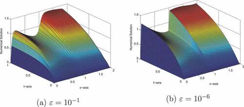
Figure 2. One dimensional plot and log-log plot for Example 7.1.

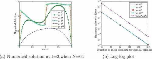
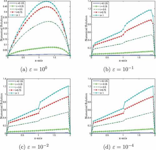
Figure 3. Numerical solution at different time levels for Example 7.1.

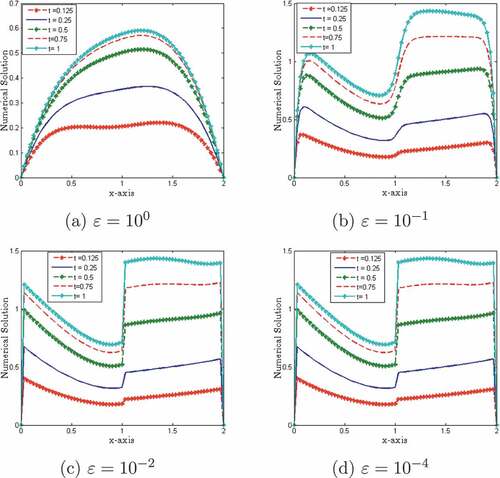
Figure 4. Surface plot of numerical solution of Example 7.2 at $N=M=128$.

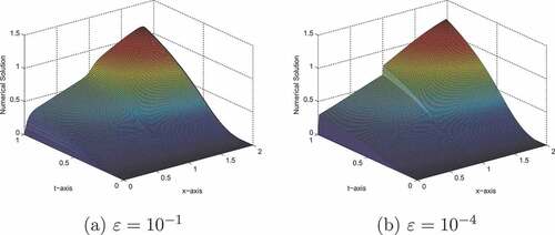
Figure 5. One dimensional plot and log-log plot for Example 7.2

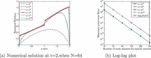
Figure 6. Numerical solution at different time levels for Example 7.2.

Example 7.1. Consider the problembrdar (Brdar et al., 2023):

(7.1) $\begin{array}{rl}& \frac{\mathrm{\partial }u}{\mathrm{\partial }t}-{\epsilon }^2\frac{{\mathrm{\partial }}^{2}u}{\mathrm{\partial }{x}^2}+2cosh(x-1)u(x,t)-(1+\frac{1}{2}{x}^2)\text{break}u(x-1,t)=e^{\frac{1}{2}x},(x,t)\in (0,2)\times (0,1],\\ & u(x,0)=0,x\in [0,2],\\ & u(x,t)=3x^2,(x,t)\in [-1,0]\times [0,1],\\ & u(2,0)=0,t\in [0,1],\end{array}$(7.1)

Example 7.2. Consider the problem (Brdar et al., 2023):

(7.2) $\begin{array}{cc}\hspace{0.17em}& \frac{\mathrm{\partial }u}{\mathrm{\partial }t}-{\epsilon }^2\frac{{\mathrm{\partial }}^{2}u}{\mathrm{\partial }{x}^2}+2cosh\left(x-1\right)u\left(x,t\right)\\ \hspace{0.17em}& -\left(1+\frac{1}{2}{x}^2\right)u\left(x-1,t\right)=f\left(x,t\right),\left(x,t\right)\in \left(0,2\right)\times \left(0,1\right],\\ \hspace{0.17em}& u\left(x,0\right)=0,x\in \left[0,2\right],\\ \hspace{0.17em}& u\left(x,t\right)=0,\left(x,t\right)\in \left[-1,0\left]\times \right[0,1\right],\\ \hspace{0.17em}& u\left(2,0\right)=0,t\in \left[0,1\right],\end{array}$(7.2)

where

(7.3) $f(x,t)=e^{\frac{1}{2}x}\left\{\begin{array}{cc}{t}^2(12-16t),& t<\frac{1}{2},\\ 1,& t\ge \frac{1}{2}.\end{array}\right.$(7.3)

The results given in Tables 1, 2, 3, 5 and 6 before and after the extrapolation technique confirm that the tabulated numerical results are in agreement with the theoretical error estimates. Figures 1, 2a and 3, and 4, 5a and 6 of the surface plot and one-dimensional plot for the numerical solution of problem in Examples 7.1 and 7.2 clearly show the behavior of the boundary layer as $\epsilon \to 0$. To demonstrate the numerical order of convergence, the maximum point-wise errors are plotted in log-log scale in 5 and 16, for Example 7.1 and Example 7.2 respectively. On the other hand, the numerical outcomes of the classical finite difference method for problem (2.1) are shown in Tables 4 and 7. From the table, it is clear that the maximum errors do not decrease significantly as the number of meshes increases; this indicates that the classical finite difference approach is not uniformly convergent.

Table 1. Computed $E_{\epsilon }^{N,M}$, $E^{N,M}$ and $R^{N,M}$ for Example 7.1, before extrapolation

	$\epsilon \downarrow$	$N/M\to$ 16/16	32/32	64/64	128/128	256/256	512/512
	${10}^{-3}$	8.5684e-04	2.4320e-04	6.4862e-05	1.6758e-05	4.2594e-06	1.0738e-06
		1.8169	1.9067	1.9525	1.9761	1.9880
	${10}^{-4}$	8.5684e-04	2.4320e-04	6.4862e-05	1.6758e-05	4.2594e-06	1.0738e-06
		1.8169	1.9067	1.9525	1.9761	1.9880
	${10}^{-5}$	8.5684e-04	2.4320e-04	6.4862e-05	1.6758e-05	4.2594e-06	1.0738e-06
		1.8169	1.9067	1.9525	1.9761	1.9880
	${10}^{-6}$	8.5684e-04	2.4320e-04	6.4862e-05	1.6758e-05	4.2594e-06	1.0738e-06
		1.8169	1.9067	1.9525	1.9761	1.9880
	${10}^{-7}$	8.5684e-04	2.4320e-04	6.4862e-05	1.6758e-05	4.2594e-06	1.0738e-06
		1.8169	1.9067	1.9525	1.9761	1.9880
	${10}^{-8}$	8.5684e-04	2.4320e-04	6.4862e-05	1.6758e-05	4.2594e-06	1.0738e-06
		1.8169	1.9067	1.9525	1.9761	1.9880
	${10}^{-9}$	8.5684e-04	2.4320e-04	6.4862e-05	1.6758e-05	4.2594e-06	1.0738e-06
		1.8169	1.9067	1.9525	1.9761	1.9880
	${10}^{-10}$	8.5684e-04	2.4320e-04	6.4862e-05	1.6758e-05	4.2594e-06	1.0738e-06
		1.8169	1.9067	1.9525	1.9761	1.9880
	${\mathbf{E}}^{\mathbf{N}\mathbf{,}\mathbf{M}}$	8.5684e-04	2.4320e-04	6.4862e-05	1.6758e-06	4.2594e-06	1.0738e-06
	${\mathbf{R}}^{\mathbf{N}\mathbf{,}\mathbf{M}}$	1.8169	1.9067	1.9525	1.9761	1.9880

Table 2. Computed $E_{\epsilon }^{N,M}$, $E^{N,M}$ and $R^{N,M}$ for Example 7.1, after extrapolation

$\epsilon \downarrow$	$N/M\to$ 16/16	32/32	64/64	128/128	256/256	512/512
${10}^{-3}$	1.1079e-06	7.7622e-08	5.1422e-09	3.4003e-10	2.1878e-11	1.3965e-12
	3.8352	3.9160	3.9187	3.9581	3.9696
${10}^{-4}$	1.1079e-06	7.7622e-08	5.1422e-09	3.4003e-10	2.1878e-11	1.3965e-12
	3.8352	3.9160	3.9187	3.9581	3.9696
${10}^{-5}$	1.1079e-06	7.7622e-08	5.1422e-09	3.4003e-10	2.1878e-11	1.3965e-12
	3.8352	3.9160	3.9187	3.9581	3.9696
${10}^{-6}$	1.1079e-06	7.7622e-08	5.1422e-09	3.4003e-10	2.1878e-11	1.3965e-12
	3.8352	3.9160	3.9187	3.9581	3.9696
${10}^{-7}$	1.1079e-06	7.7622e-08	5.1422e-09	3.4003e-10	2.1878e-11	1.3965e-12
	3.8352	3.9160	3.9187	3.9581	3.9696
${10}^{-8}$	1.1079e-06	7.7622e-08	5.1422e-09	3.4003e-10	2.1878e-11	1.3965e-12
	3.8352	3.9160	3.9187	3.9581	3.9696
${10}^{-9}$	1.1079e-06	7.7622e-08	5.1422e-09	3.4003e-10	2.1878e-11	1.3965e-12
	3.8352	3.9160	3.9187	3.9581	3.9696
${10}^{-10}$	1.1079e-06	7.7622e-08	5.1422e-09	3.4003e-10	2.1878e-11	1.3965e-12
	3.8352	3.9160	3.9187	3.9581	3.9696
${\mathbf{E}}^{\mathbf{N}\mathbf{,}\mathbf{M}}$	1.1079e-06	7.7622e-08	5.1422e-09	3.4003e-10	2.1878e-11	1.3965e-12
${\mathbf{R}}^{\mathbf{N}\mathbf{,}\mathbf{M}}$	3.8352	3.9160	3.9187	3.9581	3.9696

Table 3. Comparison for Example 7.1

Method	$\epsilon \downarrow$	$N/M\to$ 64/64	128/128	256/256	512/512
	${10}^{-2}$	7.45e-04	1.88e-04	4.74e-05	1.19e-05
(Brdar et al., 2023)		1.98	1.99	2.00
	${10}^{-4}$	7.98e-04	2.02e-04	5.13e-05	1.33e-05
		1.98	1.98	1.95
	${10}^{-6}$	2.01e-03	4.88e-04	1.36e-04	3.92e-05
		2.04	1.85	1.79
	${10}^{-10}$	2.29e-02	6.01e-03	1.66e-03	5.23e-04
		1.93	1.85	1.67
Proposed	$E^{N,M}$	6.4862e-05	1.6758e-06	4.2594e-06	1.0738e-06
before ext.	$R^{N,M}$	1.9525	1.9761	1.9880
Proposed	$E^{N,M}$	5.1422e-09	3.4003e-10	2.1878e-11	1.3965e-12
after ext.	$R^{N,M}$	3.9187	3.9581	3.9696

Table 4. Computed $E_{\epsilon }^{N,M}$ and $R^{N,M}$ for Example 7.1 using classical finite difference method(${\mu }_i(\epsilon ,h)=h$)

Method	$\epsilon \downarrow$	$N/M\to$ 16/16	32/32	64/64	128/128	256/256
before extrapolation	${10}^{-3}$	8.4795e-04	2.1577e-04	5.7871e-04	2.3376e-03	8.8871e-03
		1.9745	−1.4234	−2.0141	−1.9267
	${10}^{-4}$	8.5675e-04	2.4288e-04	6.3698e-05	2.0423e-05	9.4476e-05
		1.8186	1.9309	1.6410	−2.2097
after extrapolation	${10}^{-3}$	1.2228e-05	4.9390e-05	1.9744e-04	7.8032e-04	2.9626e-03
		2.0141	−1.9991	−1.9826	−1.9247
	${10}^{-4}$	1.1123e-06	4.9006e-07	1.9830e-06	7.9427e-06	3.1776e-05
		1.1825	−2.0166	−2.0020	−2.0002

Table 5. Computed $E_{\epsilon }^{N,M}$, $E^{N,M}$ and $R^{N,M}$ for Example 7.2 before extrapolation

$\epsilon \downarrow$	$N/M\to$ 16/16	32/32	64/64	128/128	256/256	512/512
${10}^{-3}$	1.3169e-03	3.3458e-04	8.4319e-05	2.1166e-05	5.3044e-06	1.3275e-06
	1.9767	1.9884	1.9941	1.9965	1.9985
${10}^{-4}$	1.3169e-03	3.3458e-04	8.4319e-05	2.1166e-05	5.3044e-06	1.3275e-06
	1.9767	1.9884	1.9941	1.9965	1.9985
${10}^{-5}$	1.3169e-03	3.3458e-04	8.4319e-05	2.1166e-05	5.3044e-06	1.3275e-06
	1.9767	1.9884	1.9941	1.9965	1.9985
${10}^{-6}$	1.3169e-03	3.3458e-04	8.4319e-05	2.1166e-05	5.3044e-06	1.3275e-06
	1.9767	1.9884	1.9941	1.9965	1.9985
${10}^{-7}$	1.3169e-03	3.3458e-04	8.4319e-05	2.1166e-05	5.3044e-06	1.3275e-06
	1.9767	1.9884	1.9941	1.9965	1.9985
${10}^{-8}$	1.3169e-03	3.3458e-04	8.4319e-05	2.1166e-05	5.3044e-06	1.3275e-06
	1.9767	1.9884	1.9941	1.9965	1.9985
${10}^{-9}$	1.3169e-03	3.3458e-04	8.4319e-05	2.1166e-05	5.3044e-06	1.3275e-06
	1.9767	1.9884	1.9941	1.9965	1.9985
${10}^{-10}$	1.3169e-03	3.3458e-04	8.4319e-05	2.1166e-05	5.3044e-06	1.3275e-06
	1.9767	1.9884	1.9941	1.9965	1.9985
${\mathbf{E}}^{\mathbf{N}\mathbf{,}\mathbf{M}}$	1.3169e-03	3.3458e-04	8.4319e-05	2.1166e-05	5.3044e-06	1.3275e-06
${\mathbf{R}}^{\mathbf{N}\mathbf{,}\mathbf{M}}$	1.9767	1.9884	1.9941	1.9965	1.9985

Table 6. Computed $E_{\epsilon }^{N,M}$, $E^{N,M}$ and $R^{N,M}$ for Example 7.2 after extrapolation

$\epsilon \downarrow$	$N/M\to$ 16/16	32/32	64/64	128/128	256/256	512/512
${10}^{-3}$	2.4632e-06	1.5858e-07	1.0075e-08	6.3485e-10	3.9846e-11	2.5036e-12
	3.9572	3.9763	3.9883	3.9939	3.9924
${10}^{-4}$	2.4632e-06	1.5858e-07	1.0075e-08	6.3485e-10	3.9846e-11	2.5036e-12
	3.9572	3.9763	3.9883	3.9939	3.9924
${10}^{-5}$	2.4632e-06	1.5858e-07	1.0075e-08	6.3485e-10	3.9846e-11	2.5036e-12
	3.9572	3.9763	3.9883	3.9939	3.9924
${10}^{-6}$	2.4632e-06	1.5858e-07	1.0075e-08	6.3485e-10	3.9846e-11	2.5036e-12
	3.9572	3.9763	3.9883	3.9939	3.9924
${10}^{-7}$	2.4632e-06	1.5858e-07	1.0075e-08	6.3485e-10	3.9846e-11	2.5036e-12
	3.9572	3.9763	3.9883	3.9939	3.9924
${10}^{-8}$	2.4632e-06	1.5858e-07	1.0075e-08	6.3485e-10	3.9846e-11	2.5036e-12
	3.9572	3.9763	3.9883	3.9939	3.9924
${10}^{-9}$	2.4632e-06	1.5858e-07	1.0075e-08	6.3485e-10	3.9846e-11	2.5036e-12
	3.9572	3.9763	3.9883	3.9939	3.9924
${10}^{-10}$	2.4632e-06	1.5858e-07	1.0075e-08	6.3485e-10	3.9846e-11	2.5036e-12
	3.9572	3.9763	3.9883	3.9939	3.9924
$E^{N,M}$	2.4632e-06	1.5858e-07	1.0075e-08	6.3485e-10	3.9846e-11	2.5036e-12
$R^{N,M}$	3.9572	3.9763	3.9883	3.9939	3.9924

Table 7. Computed $E_{\epsilon }^{N,M}$ and $R^{N,M}$ for Example 7.2 using classical finite difference method(${\mu }_i(\epsilon ,h)=h$)

Method	$\epsilon \downarrow$	$N/M\to$ 16/16	32/32	64/64	128/128	256/256
before extrapolation	${10}^{-3}$	1.3167e-03	3.3393e-04	3.0137e-04	1.1132e-03	4.2428e-03
		1.9793	1.4800	−1.8851	−1.9303
	${10}^{-4}$	1.3169e-03	3.3457e-04	8.4294e-05	2.1649e-05	4.5982e-05
		1.9767	1.9888	1.9611	−1.0867
after extrapolation	${10}^{-3}$	4.9576e-06	2.3776e-05	9.3936e-05	3.6945e-04	1.4139e-03
		−2.2618	−1.9822	−1.9756	−1.9362
	${10}^{-4}$	2.4491e-06	1.6465e-07	9.3794e-07	3.7449e-06	1.4924e-05
		3.8948	−2.5101	−1.9974	−1.9947

8 Conclusion

A singularly perturbed reaction diffusion problem of large spatial delay is treated via a non-standard finite difference method in the spatial direction and the Crank—Nicolson method for time derivative is applied. Due to the presence of a small perturbation parameter, the problem exhibits left- and right-side boundary layers at $x=0$ and $x=2$ respectively. In addition to these, because of the appearance of the large delay, there is an interior layer at $x=1$. To obtain higher accuracy and higher order of convergence, Richardson extrapolation is employed. The convergence analysis of the proposed scheme is discussed, and the scheme is $\epsilon -$ uniform convergent of fourth order accurate in both time and space variables. The efficiency of the proposed scheme is tested on two specific examples. The numerical outcomes indicate that the results are in agreement with the theoretical results. Moreover, comparison is made, and it is observed that the proposed scheme gives more accurate as well as a higher rate of convergence as compared to study available in the literature.

Disclosure statement

No potential conflict of interest was reported by the author(s).

Additional information

Funding

The authors received no direct funding for this research.

Notes on contributors

Awoke Andargie Tiruneh

Awoke Andargie Tiruneh received his Ph.D. and Post-Doc in mathematics from the NIT, Warangal, India. He is presently working at Bahir Dar University as an associate professor. His research interests are in the areas of applied mathematics and numerical analysis, including the theory of perturbation. He has done several publications in different reputed journal.

Getachew Adamu Derese

Getachew Adamu Derese received his Ph.D. in mathematics from IIT Kanpur, India. He is presently working at Bahir Dar University, Ethiopia, as an associate professor. His research interests are in the areas of applied mathematics and numerical analysis, including the lubrication of bearings. He has done several publications in different reputed journal.

Mulunesh Amsalu Ayele

Mulunesh Amsalu Ayele is a Ph.D. candidate at Bahir Dar University, Ethiopia. Her research interests are in the area of applied mathematics and numerical analysis, including the numerical solution of singularly perturbed differential equations.

References

- Ayele, M. A., Tiruneh, A. A., & Derese, G. A. (2022). Fitted scheme for singularly perturbed time delay reaction-diffusion problems. Iranian Journal of Numerical Analysis and Optimization. https://doi.org/10.22067/ijnao.2022.77453.1161
- Ayele, M. A., Tiruneh, A. A., Derese, G. A., & Araci, S. (2022). Uniformly convergent scheme for singularly perturbed space delay parabolic differential equation with discontinuous convection coefficient and source term. Journal of Mathematics, 2022, 1–15. https://doi.org/10.1155/2022/1874741
- Babu, G., & Bansal, K. (2022). A high order robust numerical scheme for singularly perturbed delay parabolic convection diffusion problems. Journal of Applied Mathematics and Computing, 68(1), 363–389. https://doi.org/10.1007/s12190-021-01512-1
- Bansal, K., Rai, P., & Sharma, K. K. (2017). Numerical treatment for the class of time dependent singularly perturbed parabolic problems with general shift arguments. Differential Equations and Dynamical Systems, 25(2), 327–346. https://doi.org/10.1007/s12591-015-0265-7
- Bansal, K., & Sharma, K. K. (2017). Parameter uniform numerical scheme for time dependent singularly perturbed convection-diffusion-reaction problems with general shift arguments. Numerical Algorithms, 75(1), 113–145. https://doi.org/10.1007/s11075-016-0199-3
- Bansal, K., & Sharma, K. K. (2018). Parameter-robust numerical scheme for time-dependent singularly perturbed reaction–diffusion problem with large delay. Numerical Functional Analysis and Optimization, 39(2), 127–154. https://doi.org/10.1080/01630563.2016.1277742
- Brdar, M., Franz, S., Ludwig, L., & Roos, H. G. (2023). A balanced norm error estimation for the time-dependent reaction-diffusion problem with shift in space. Applied Mathematics and Computation, 437, 127507. https://doi.org/10.1016/j.amc.2022.127507
- Burcu, G. (2021). A computational technique for solving singularly perturbed delay partial differential equations. Foundations of Computing and Decision Sciences, 46(3), 221–233. https://doi.org/10.2478/fcds-2021-0015
- Choudhary, M., & Kaushik, A. (2022). A uniformly convergent defect correction method for parabolic singular perturbation problems with a large delay. Journal of Applied Mathematics and Computing, 1–25. https://doi.org/10.1007/s12190-022-01796-x
- Clavero, C., & Gracia, J. L. (2010). On the uniform convergence of a finite difference scheme for time dependent singularly perturbed reaction-diffusion problems. Applied Mathematics and Computation, 216(5), 1478–1488. https://doi.org/10.1016/j.amc.2010.02.050
- Daba, I. T., & Duressa, G. F. (2021). Hybrid algorithm for singularly perturbed delay parabolic partial differential equations. Applications and Applied Mathematics: An International Journal (AAM), 16(1), 21. https://digitalcommons.pvamu.edu/aam/vol16/iss1/21
- Duressa, G. F., & Woldaregay, M. M. (2022). Fitted numerical scheme for solving singularly perturbed parabolic delay partial differential equations. Tamkang Journal of Mathematics, 53. https://doi.org/10.5556/j.tkjm.53.2022.3638
- Ejere, A. H., Duressa, G. F., Woldaregay, M. M., & Dinka, T. G. (2022). A uniformly convergent numerical scheme for solving singularly perturbed differential equations with large spatial delay. SN Applied Sciences, 4(12), 1–15. https://doi.org/10.1007/s42452-022-05203-9
- Elango, S., Tamilselvan, A., Vadivel, R., Gunasekaran, N., Zhu, H., Cao, J., & Xiaodi, L. (2021). Finite difference scheme for singularly perturbed reaction diffusion problem of partial delay differential equation with nonlocal boundary condition. Advances in Difference Equations, 2021(1), 1–20. https://doi.org/10.1186/s13662-021-03296-x
- Gelu, F. W., Duressa, G. F., & Kovtunenko, V. (2021). A uniformly convergent collocation method for singularly perturbed delay parabolic reaction-diffusion problem.abstract and Applied Analysis, 2021, 1–11. Hindawi. https://doi.org/10.1155/2021/8835595
- Gobena, W. T., Duressa, G. F., & Scapellato, A. (2021). Parameter-uniform numerical scheme for singularly perturbed delay parabolic reaction diffusion equations with integral boundary condition. International Journal of Differential Equations, 2021, 1–16. https://doi.org/10.1155/2021/9993644
- Govindarao, L., Mohapatra, J., & Das, A. (2020). A fourth-order numerical scheme for singularly perturbed delay parabolic problem arising in population dynamics. Journal of Applied Mathematics and Computing, 63(1), 171–195. https://doi.org/10.1007/s12190-019-01313-7
- Hailu, W. S., Duressa, G. F., & Liu, L. (2022). Parameter- uniform cubic spline method for singularly perturbed parabolic differential equation with large negative shift and integral boundary condition. Research in Mathematics, 9(1), 2151080. https://doi.org/10.1080/27684830.2022.2151080
- Kaushik, A., & Sharma, N. (2020). An adaptive difference scheme for parabolic delay differential equation with discontinuous coefficients and interior layers. Journal of Difference Equations and Applications, 26(11–12), 1450–1470. https://doi.org/10.1080/10236198.2020.1843645
- Kumar, D. (2021). A parameter-uniform scheme for the parabolic singularly perturbed problem with a delay in time. Numerical Methods for Partial Differential Equations, 37(1), 626–642. https://doi.org/10.1002/num.22544
- Kumar, K., Gupta, T., Pramod Chakravarthy, P., & Nageshwar Rao, R. (2019). An adaptive mesh selection strategy for solving singularly perturbed parabolic partial differential equations with a small delay. In. Applied Mathematics and Scientific Computing, Springer, 67–76. https://doi.org/10.1007/978-3-030-01123-9_8
- Kumar, D., & Kadalbajoo, M. K. (2011). A parameter-uniform numerical method for time-dependent singularly perturbed differential-difference equations. Applied Mathematical Modelling, 35(6), 2805–2819. https://doi.org/10.1016/j.apm.2010.11.074
- Kumar, D., & Kumari, P. (2019). A parameter-uniform numerical scheme for the parabolic singularly perturbed initial boundary value problems with large time delay. Journal of Applied Mathematics and Computing, 59(1), 179–206. https://doi.org/10.1007/s12190-018-1174-z
- Kumar, D., & Kumari, P. (2020). Parameter-uniform numerical treatment of singularly perturbed initial-boundary value problems with large delay. Applied Numerical Mathematics, 153, 412–429. https://doi.org/10.1016/j.apnum.2020.02.021
- Ladyzhenskaia, O. A., Solonnikov, V. A., & Ural’tseva, N. N. (1988). Linear and quasi-linear equations of parabolic type (Vol. 23). American Mathematical Soc.
- Lange, C. G., & Miura, R. M. (1994). Singular perturbation analysis of boundary value problems for differential-difference equations. v. small shifts with rapid oscillations. SIAM Journal on Applied Mathematics, 54(1), 273–283. https://doi.org/10.1137/s0036139992228119
- Manikandan, M., Shivaranjani, N., Miller, J. J. H., & Valarmathi, S. (2014). A parameter- uniform numerical method for a boundary value problem for a singularly perturbed delay differential equation. Advances in Applied Mathematics Springer 71–88. https://doi.org/10.1007/978-3-319-06923-4_7
- Mickens, R. E. (1994). Nonstandard finite difference models of differential equations. world scientific.
- Mukherjee, K., & Natesan, S. (2010, October). Richardson extrapolation technique for singularly perturbed parabolic convection–diffusion problems. Computing, 92(1), 1–32. https://doi.org/10.1007/s00607-010-0126-8
- Musila, M., & Petr, L. (1991). Generalized stein’s model for anatomically complex neurons. BioSystems, 25(3), 179–191. https://doi.org/10.1016/0303-2647(91)90004-5
- Negero, N. T., & Duressa, G. F. (2022). Uniform convergent solution of singularly perturbed parabolic differential equations with general temporal- lag. Iranian Journal of Science and Technology, Transactions A: Science, 46(2), 507–524. https://doi.org/10.1007/s40995-021-01258-2
- Parthiban, S., Valarmathi, S., & Franklin, V. (2015). A numerical method to solve singularly perturbed linear parabolic second order delay differential equation of reaction-diffusion type. Malaya J Matematik, 412–420.
- Prathap, T., & Nageshwar Rao, R. (2022). Uniformly convergent finite difference methods for singularly perturbed parabolic partial differential equations with mixed shifts. Journal of Applied Mathematics and Computing, 1–26. https://doi.org/10.1007/s12190-022-01802-2
- Ramesh, V. P., & Kadalbajoo, M. K. (2008). Upwind and midpoint upwind difference methods for time-dependent differential difference equations with layer behavior. Applied Mathematics and Computation, 202(2), 453–471. https://doi.org/10.1016/j.amc.2007.11.033
- Roos, H.-G., Stynes, M., & Tobiska, L. (2008). Robust numerical methods for singularly perturbed differential equations: Convection-diffusion-reaction and flow problems (Vol. 24). Springer Science & Business Media.
- Stein, R. B. (1965). A theoretical analysis of neuronal variability. Biophysical Journal, 5(2), 173–194. https://doi.org/10.1016/S0006-3495(65)86709-1
- Stein, R. B. (1967). Some models of neuronal variability. Biophysical Journal, 7(1), 37–68. https://doi.org/10.1016/S0006-3495(67)86574-3
- Woldaregay, M. M., Duressa, G. F., & Scapellato, A. (2021). Uniformly convergent hybrid numerical method for singularly perturbed delay convection- diffusion problems. International Journal of Differential Equations, 2021, 1–20. https://doi.org/10.1155/2021/6654495