Certain results on generalized Humbert-Hermite polynomials

ABSTRACT

In this article, we introduce a new class of generalized Humbert-Hermite polynomials of two variables. We are conscious that the present paper was inspired by a unified presentation of a class of two-variable Humbert’s polynomials that generalize the well-known class of Gegenbauer, Humbert, Legendre, Chebycheff, Pincherle, Horadam, Kinnsy, Horadam-Pethe, Djordjevi’c, Gould, Milovanovi’c and Djordjevi’c, Pathan, and Khan polynomials. Also, we present well-known results by analyzing the particular values of the parameter. We give the surface representation of a generalized Humbert-Hermite polynomial using some particular values of the parameters.

KEYWORDS:

• Hermite polynomials
• Humbert polynomials
• Gegenbauer polynomials
• Chebyshev polynomials
• Pathan-khan polynomials
• hypergeometric function

1. Introduction and preliminaries

The concept defines special polynomials formed from the solutions of differential equations under specified conditions. Special polynomials can be represented in various ways, including generating function, p-adic integrals, recurrence relations, degenerate versions and so on. The theory of finite differences, analytic number theory, classical analysis and statistics are the most significant polynomials applications. The present article defines a new class of generalized Humbert-Hermite polynomials of two variables and discusses their remarkable as well as some special cases. We are conscious that the present article was inspired by a unified presentation of a class of two-variable Humbert’s polynomials that generalize the well-known class of Gegenbauer, Humbert, Legendre, Chebycheff, Pincherle, Horadam, Kinnsy, Horadam-Pethe, Djordjevi’c, Gould, Milovanovi’c and Djordjevi’c, Pathan and Khan polynomials. Also, we present well-known results by analyzing the particular values of the parameter. We give the surface representation of a generalized Humbert-Hermite polynomial using some particular values of the parameters.

The two-variable Hermite polynomials (or Kampé de Fériet) (Bell, 1934; Dattoli, Lorenzutta, et al., 1999) are defined by

(1.1) ${\mathcal{H}}_{\mathit{\eta }}(\mathit{\alpha },\mathit{\beta })=\mathit{\eta }!\sum _{\mathit{r}=0}^{\left[\frac{\eta }{2}\right]}\frac{{\mathit{\beta }}^{\mathit{r}}{\alpha }^{\mathit{\eta }-2\mathit{r}}}{\mathit{r}!(\mathit{\eta }-2\mathit{r})!}.$(1.1)

These polynomials are usually defined by means of their generating function

(1.2) $e^{\alpha \ell +\beta {\ell }^2}=\sum _{\mathit{\eta }=0}^{\mathrm{\infty }}{\mathcal{H}}_{\eta }(\mathit{\alpha },\mathit{\beta })\frac{{\ell }^{\mathit{\eta }}}{\mathit{\eta }!},$(1.2)

when $\mathit{\beta }=-1$ and α is replaced by 2α, it reduces to the ordinary Hermite polynomials ${\mathcal{H}}_{\eta }(\mathit{\alpha })$ (see (Andrews, 1985)).

Now, we recall the definition of N-variable generalized Hermite polynomials ${\mathcal{H}}_{\eta }(\{\mathit{\alpha }{\}}_1^N)$ defined by ((Dattoli et al., 1996), p.602) :

(1.3) $\mathit{exp}\sum _{\mathit{i}=1}^{\mathit{N}}{x}_i{\ell }^i=\sum _{\mathit{\eta }=0}^{\mathrm{\infty }}{\mathcal{H}}_{\eta }(\{\mathit{\alpha }{\}}_1^N)\frac{{\ell }^{\eta }}{\mathit{\eta }!},$(1.3)

where $(\{\mathit{\alpha }{\}}_1^N)$ = ${\alpha }_1,{\alpha }_2,\dots ,{\alpha }_{\mathit{N}}.$

The generalized Hermite polynomials ${\mathcal{H}}_{\eta }(\{\mathit{\alpha }{\}}_1^N)$ for N = 3 also belong to the Bell type as shown in ((Dattoli, Torre, et al., 1999), p.403(26)). The Gould-Hopper polynomials $g_{\eta }^m(\mathit{\alpha },\mathit{\beta })$ (see (Dattoli et al., 1993) and (Djordjevic & Milovanovic, 2014)) are a special case of (1.3). The notation ${\mathcal{H}}_{\eta }^m(\mathit{\alpha },\mathit{\beta })$ or $g_{\eta }^m(\mathit{\alpha },\mathit{\beta })$ was given by (Dattoli et al., 1993). These are specified by

(1.4) $e^{\mathit{\alpha \ell }+\beta {\ell }^m}=\sum _{\mathit{\eta }=0}^{\mathrm{\infty }}{\mathcal{H}}_{\eta }^m(\mathit{\alpha },\mathit{\beta })\frac{{\ell }^{\mathit{\eta }}}{\mathit{\eta }!}.$(1.4)

Another generalization of Hermite polynomials is given by ${\mathcal{H}}_{\mathit{\eta },\mathit{m},\mathit{\mu }}(\mathit{\alpha },\mathit{\beta })$ in the form of the generating function (see (Pathan & Khan, 1997))

(1.5) $e^{\mathit{\gamma }(\mathit{\alpha }+\mathit{\beta })\mathit{\ell }-(\mathit{\alpha \beta }+1){\mathit{\ell }}^{\mathit{m}}}=\sum _{\mathit{\eta }=0}^{\mathrm{\infty }}{\mathcal{H}}_{\mathit{\eta },\mathit{m},\mathit{\gamma }}(\mathit{\alpha },\mathit{\beta })\frac{{\ell }^{\mathit{\eta }}}{\mathit{\eta }!},$(1.5)

when γ = 2, α = 0 or $\mathit{\gamma }=2$, β = 0, (1.5(1.5) $e^{\mathit{\gamma }(\mathit{\alpha }+\mathit{\beta })\mathit{\ell }-(\mathit{\alpha \beta }+1){\mathit{\ell }}^{\mathit{m}}}=\sum _{\mathit{\eta }=0}^{\mathrm{\infty }}{\mathcal{H}}_{\mathit{\eta },\mathit{m},\mathit{\gamma }}(\mathit{\alpha },\mathit{\beta })\frac{{\ell }^{\mathit{\eta }}}{\mathit{\eta }!},$(1.5) ) reduces to the ordinary Hermite polynomials ${\mathcal{H}}_{\eta }(\mathit{\alpha })$.

We give some attention to familiar generating relations

(1.6) $(1-2\mathit{\alpha \ell }+{\ell }^2{)}^{-\frac{1}{2}}=\sum _{\mathit{\eta }=0}^{\mathrm{\infty }}{\mathcal{P}}_{\mathit{\eta }}(\mathit{\alpha })\frac{{\ell }^{\mathit{\eta }}}{\mathit{\eta }!},$(1.6)

where ${\mathcal{P}}_{\mathit{\eta }}(\mathit{\alpha })$ is Lagendre’s polynomial (see (Rainville, 1960), p. no. 157) of the first kind

(1.7) $(1-2\mathit{\alpha \ell }+{\ell }^2{)}^{-1}=\sum _{\mathit{\eta }=0}^{\mathrm{\infty }}{\mathcal{U}}_{\mathit{\eta }}(\mathit{\alpha })\frac{{\ell }^{\mathit{\eta }}}{\mathit{\eta }!},$(1.7)

where ${\mathcal{U}}_{\mathit{\eta }}(\mathit{\alpha })$ is Chebychev polynomial (see (Rainville, 1960), p. 301, eq. no. 3) of the second kind

(1.8) $(1-2\mathit{\alpha \ell }+{\ell }^2{)}^{-\mathit{\mu }}=\sum _{\mathit{\eta }=0}^{\mathrm{\infty }}{\mathcal{C}}_{\eta }^{\mu }(\mathit{\alpha })\frac{{\ell }^{\mathit{\eta }}}{\mathit{\eta }!},$(1.8)

where ${\mathcal{C}}_{\eta }^{\mu }(\mathit{\alpha })$ is Gegenbauer’s polynomial (see (Rainville, 1960), page no. 276).

(1.9) $(1-2\mathit{\alpha \ell }+{\ell }^m{)}^{-\mathit{\mu }}=\sum _{\mathit{\eta }=0}^{\mathrm{\infty }}{\mathfrak{h}}_{\eta ,m}^{\mu }(\mathit{x})\frac{{\ell }^{\mathit{\eta }}}{\mathit{\eta }!},$(1.9)

${\mathfrak{h}}_{\eta ,m}^{\mu }(\mathit{\alpha })=\sum _{\mathit{\kappa }=0}^{\left[\frac{\eta }{m}\right]}\frac{(-1{)}^{\mathit{\kappa }}(\mathit{\mu }{)}_{\mathit{\eta }+(1-\mathit{m})\mathit{\kappa }}(\mathit{m\alpha }{)}^{\mathit{\eta }-\mathit{m\kappa }}}{\mathit{\eta }!(\mathit{\eta }-\mathit{m\kappa })!},$

where ${\mathfrak{h}}_{\eta ,m}^{\mu }(\mathit{\alpha })$ is the Humbert polynomial and m is a positive integer. The Pochhammer symbol $(\mathit{b}{)}_{\mathit{\eta }}$ is defined by

$\begin{array}{ll}(\mathit{b}{)}_{\eta }& =\frac{\mathrm{\Gamma }(\mathit{b}+\mathit{\eta })}{\mathrm{\Gamma }(\mathit{b})}\\ =\left[\begin{array}{ll}1;& \mathit{if}\mathit{\eta }=0\\ (\mathit{b})(\mathit{b}+1)(\mathit{b}+2)(\mathit{b}+\mathit{\eta }-1);& \mathit{if\eta }=1,2,3,\end{array}\right]\end{array}$

In 1965, Gould, (1965) gave the following generating relation

(1.10) $(\mathit{c}-\mathit{m\alpha \ell }+\mathit{\beta }{\ell }^m{)}^{\mathit{\rho }}=\sum _{\mathit{\eta }=0}^{\mathrm{\infty }}{\mathcal{P}}_{\mathit{\eta }}(\mathit{m},\mathit{\alpha },\mathit{\beta },\mathit{\rho },\mathit{c}){\ell }^{\mathit{\eta }},$(1.10)

where m will be a positive integer and other parameters are unrestricted in sign.

The ${\mathcal{P}}_{\eta }(\mathit{m},\mathit{\alpha },\mathit{\beta },\mathit{\rho },\mathit{c})$ is defined explicitly as ((Gould, 1965), p.699):

(1.11) $\begin{array}{ll}{\mathcal{P}}_{\eta }(\mathit{m},\mathit{\alpha },\mathit{\beta },\mathit{\rho },\mathit{c})=& \sum _{\mathit{\kappa }=0}^{\left[\frac{\eta }{m}\right]}(\genfrac{}{}{0ex}{}{\eta }{\kappa })(\genfrac{}{}{0ex}{}{\mathit{\rho }-\mathit{\kappa }}{\mathit{\eta }-\mathit{m\kappa }})c^{\mathit{\rho }-\mathit{\eta }+(\mathit{m}-1)\mathit{\kappa }}\\ \times {\beta }^{\mathit{\kappa }}(-\mathit{m\alpha }{)}^{\mathit{\eta }-\mathit{m\kappa }}.\end{array}$(1.11)

In 1989, Sinha, (1989) gave the following generating relation

(1.12) $[1-2\mathit{\alpha \ell }+{\ell }^2(2\mathit{\alpha }-1){]}^{-\mathit{\mu }}=\sum _{\mathit{\eta }=0}^{\mathrm{\infty }}{\mathcal{S}}_{\eta }^{\mu }(\mathit{\alpha }){\ell }^{\mathit{\eta }},$(1.12)

where

(1.13) ${\mathcal{S}}_{\eta }^{\mu }(\mathit{\alpha })=\sum _{\mathit{\kappa }=0}^{\left[\frac{\eta }{m}\right]}\frac{(-1{)}^{\mathit{\kappa }}(\mathit{\mu }{)}_{\mathit{\eta }-\mathit{\kappa }}(2\mathit{\alpha }{)}^{\mathit{\eta }-2\mathit{\kappa }}(2\mathit{\alpha }-1{)}^{\kappa }}{\mathit{\kappa }!(\mathit{\eta }-2\mathit{\kappa })!},$(1.13)

${\mathcal{S}}_{\eta }^{\mu }(\mathit{\alpha })$ is the generalization of Shrestha polynomial ${\mathcal{S}}_{\eta }(\mathit{\alpha })$ (see (Pathan & Khan, 1997)).

In 1991, Milovanovic & Djordjevic, (1987) (see also (Milovanovic & Djordjevic, 1991)) gave the following generating relation

(1.14) $(1-2\mathit{\alpha \ell }+{\ell }^m{)}^{-\mathit{\lambda }}=\sum _{\mathit{\eta }=0}^{\mathrm{\infty }}{\mathcal{P}}_{\eta ,m}^{\lambda }(\mathit{\alpha }){\ell }^{\mathit{\eta }},$(1.14)

where $\mathit{m}\in \mathbb{N}$ and $\mathit{\lambda }>\frac{-1}{2}$ and

(1.15) ${\mathcal{P}}_{\eta ,m}^{\lambda }(\mathit{\alpha })=\sum _{\mathit{\kappa }=0}^{\left[\frac{\eta }{m}\right]}\frac{(-1{)}^{\mathit{\kappa }}(\mathit{\lambda }{)}_{\mathit{\eta }-(\mathit{m}-1)\mathit{\kappa }}(2\mathit{\alpha }{)}^{\mathit{\eta }-\mathit{m\kappa }}}{\mathit{\kappa }!(\mathit{\eta }-\mathit{m\kappa })!},$(1.15)

It is to be noted that the polynomials represented by ${\mathcal{P}}_{\eta ,1}^{\lambda }(\mathit{\alpha })$, ${\mathcal{P}}_{\eta ,2}^{\lambda }(\mathit{\alpha })$ and ${\mathcal{P}}_{\eta ,3}^{\lambda }(\mathit{\alpha })$ are known as Horadam polynomials (Horadam, 1985), Gegenbauer polynomials (Rainville, 1960) and Horadam-Pethe polynomials (Horadam & Pethe, 1981), respectively. Many interesting generalizations of these polynomials appeared in the literature.

In particular, in 1997, Pathan & Khan, (1997), p.54) generalized these polynomials and gave the following generating relation

(1.16) $\begin{array}{ll} [\mathit{c}-\mathit{a\alpha \ell }+\mathit{b}{\ell }^m(2\mathit{\alpha }-1{)}^d{]}^{-\mathit{\mu }}& =\sum _{\mathit{\eta }=0}^{\mathrm{\infty }}{\mathcal{P}}_{\eta ,m,a,b,c,d}^{\mu }(\mathit{\alpha }){\ell }^{\mathit{\eta }}\\ =\sum _{\mathit{\eta }=0}^{\mathrm{\infty }}{\mathrm{\Theta }}_{\mathit{\eta }}(\mathit{\alpha }){\ell }^{\eta },\end{array}$(1.16)

where

(1.17) $\begin{array}{l}{\mathrm{\Theta }}_{\eta }(\mathit{\alpha }){\ell }^{\eta }\\ =\sum _{\mathit{\kappa }=0}^{[\frac{\eta }{m}]}\frac{{(-1)}^{\kappa }{c}^{-\mathit{\mu }-\mathit{n}+(\mathit{m}-1)\mathit{\kappa }}{(\mathit{\mu })}_{\mathit{n}+(1-\mathit{m})\mathit{\kappa }}{(\mathit{a\alpha })}^{\mathit{\eta }-\mathit{m\kappa }}{[\mathit{b}{(2\mathit{\alpha }-1)}^d]}^{\mathit{\kappa }}}{\mathit{\eta }!(\mathit{\eta }-\mathit{m\kappa })!}.\end{array}$(1.17)

Djordjevic () provided a generalization of various polynomials of two variables in the form

(1.18) $[1-2(\mathit{\alpha }+\mathit{\beta })\mathit{\ell }+{\ell }^m(2\mathit{\alpha \beta }+1){]}^{-\mathit{\gamma }}=\sum _{\mathit{\eta }=0}^{\mathrm{\infty }}{\mathcal{G}}_{\eta }^{\gamma ,m}(\mathit{\alpha },\mathit{\beta }){\ell }^{\mathit{\eta }},$(1.18)

where

(1.19) $\begin{array}{l}{\mathcal{G}}_{\eta }^{\gamma ,m}(\mathit{\alpha },\mathit{\beta }){\ell }^{\mathit{\eta }}\\ =\sum _{\mathit{\kappa }=0}^{\left[\frac{\eta }{m}\right]}\frac{(-1{)}^{\mathit{\kappa }}(\mathit{\gamma }{)}_{\mathit{\eta }-(\mathit{m}-1)\mathit{\kappa }}(2\mathit{\alpha }+2\mathit{\beta }{)}^{\mathit{\eta }-\mathit{m\kappa }}(2\mathit{\alpha \beta }+1{)}^{\kappa }}{\mathit{\eta }!(\mathit{\eta }-\mathit{m\kappa })!}.\end{array}$(1.19)

Note that ${\mathcal{G}}_{\eta }^{1,m}(\mathit{\alpha },\mathit{\beta })$ = ${\mathcal{G}}_{\eta }^m(\mathit{\alpha },\mathit{\beta })$ and ${\mathcal{G}}_{\mathit{\eta }}^{\frac{1}{2},\mathit{m}}(\mathit{\alpha },\mathit{\beta })$ = ${\mathcal{P}}_{\eta }^m(\mathit{\alpha },\mathit{\beta })$ where ${\mathcal{C}}_{\eta }^m(\mathit{\alpha },\mathit{\beta })$ and ${\mathcal{U}}_{\eta }^m(\mathit{\alpha },\mathit{\beta })$ are Chebyshev and Legendre polynomials of two variables respectively.

For m = 2, ${\mathcal{G}}_{\eta }^{\gamma ,m}(\mathit{\alpha },\mathit{\beta })$ reduces to a polynomial studied by (Dave, 1978)]. For m = 2 and β = 0, ${\mathcal{G}}_{\eta }^{\gamma ,m}(\mathit{\alpha },\mathit{\beta })$ reduces to a Gegenbauer polynomial and for m = 3 and β = 0, ${\mathcal{G}}_{\eta }^{\gamma ,m}(\mathit{\alpha },\mathit{\beta })$ are Horadam-Pethe polynomial (Horadam & Pethe, 1981). Further, for β = 0, ${\mathcal{G}}_{\eta }^{\gamma ,m}(\mathit{\alpha },\mathit{\beta })$ reduces to a polynomial ${\mathcal{P}}_{\eta ,m}^{\gamma }(\mathit{\alpha })$ studied by Milovanovic & Djordjevic, (1987) and Milovanovic & Djordjevic, (1991).

A generalization and unification of various polynomials mentioned above is provided by the definition of generalized Humbert polynomials in two variables given recently by Pathan & Khan, (2015) which has the generating function

(1.20) $\begin{array}{l}[\mathit{a}-(\mathit{b\alpha }+\mathit{c\beta })\mathit{\ell }+\mathit{d}{\ell }^m(\mathit{e\alpha \beta }-1{)}^g{]}^{-\mathit{\mu }}\\ =\sum _{\mathit{\eta }=0}^{\mathrm{\infty }}{\mathcal{Q}}_{\eta ,m,g,\mu }^{a,b,c,d,e}(\mathit{\alpha },\mathit{\beta }){\ell }^{\mathit{\eta }}\end{array}$(1.20)

where $\mathit{m}\in \mathbb{N}$ and h > 0 and the other parameters are unrestricted in general.

In (1.20(1.20) $\begin{array}{l}[\mathit{a}-(\mathit{b\alpha }+\mathit{c\beta })\mathit{\ell }+\mathit{d}{\ell }^m(\mathit{e\alpha \beta }-1{)}^g{]}^{-\mathit{\mu }}\\ =\sum _{\mathit{\eta }=0}^{\mathrm{\infty }}{\mathcal{Q}}_{\eta ,m,g,\mu }^{a,b,c,d,e}(\mathit{\alpha },\mathit{\beta }){\ell }^{\mathit{\eta }}\end{array}$(1.20) ), if we put a = 1, $\mathit{b}=\mathit{c}=2$, $\mathit{d}=-1$, $\mathit{e}=-2$ and g = 1, then we get a generating relation (1.18(1.18) $[1-2(\mathit{\alpha }+\mathit{\beta })\mathit{\ell }+{\ell }^m(2\mathit{\alpha \beta }+1){]}^{-\mathit{\gamma }}=\sum _{\mathit{\eta }=0}^{\mathrm{\infty }}{\mathcal{G}}_{\eta }^{\gamma ,m}(\mathit{\alpha },\mathit{\beta }){\ell }^{\mathit{\eta }},$(1.18) ) studied by (Djordjevic). For β = 1, e = 2 and c = 0, we get a generating relation (1.16(1.16) $\begin{array}{ll} [\mathit{c}-\mathit{a\alpha \ell }+\mathit{b}{\ell }^m(2\mathit{\alpha }-1{)}^d{]}^{-\mathit{\mu }}& =\sum _{\mathit{\eta }=0}^{\mathrm{\infty }}{\mathcal{P}}_{\eta ,m,a,b,c,d}^{\mu }(\mathit{\alpha }){\ell }^{\mathit{\eta }}\\ =\sum _{\mathit{\eta }=0}^{\mathrm{\infty }}{\mathrm{\Theta }}_{\mathit{\eta }}(\mathit{\alpha }){\ell }^{\eta },\end{array}$(1.16) ) studied by Pathan & Khan, (1997). For a = 1, b = 2, c = 0, d = 1 and g = 0, we get a generating relation (1.14(1.14) $(1-2\mathit{\alpha \ell }+{\ell }^m{)}^{-\mathit{\lambda }}=\sum _{\mathit{\eta }=0}^{\mathrm{\infty }}{\mathcal{P}}_{\eta ,m}^{\lambda }(\mathit{\alpha }){\ell }^{\mathit{\eta }},$(1.14) ) studied by Milovanovic & Djordjevic, (1991). For a = 1, b = 2, m = 2, y = 1, e = 2 and g = 1, we get a polynomial defined by Sinha, (1989) and for c = 0, g = 0, d = y and $\mathit{h}=-\mathit{\rho }$, we get a generating relation (1.4(1.4) $e^{\mathit{\alpha \ell }+\beta {\ell }^m}=\sum _{\mathit{\eta }=0}^{\mathrm{\infty }}{\mathcal{H}}_{\eta }^m(\mathit{\alpha },\mathit{\beta })\frac{{\ell }^{\mathit{\eta }}}{\mathit{\eta }!}.$(1.4) ) given by Gould, (1965). Some more interesting special cases which are recorded by Djordjevic & Milovanovic, (2014) can be established similarly.

Recently, Khan & Pathan, (2021) gave generalized Humbert-Hermite polynomials in two variables ${\mathit{ }}_{\mathcal{H}}{\mathcal{G}}_{\eta }^{\mu ,\gamma ,m}(\mathit{\alpha },\mathit{\beta })$, which has the generating function as follows:

(1.21) $\begin{array}{l}[1-2(\mathit{\alpha }+\mathit{\beta })\mathit{\ell }+{\ell }^m(2\mathit{\alpha \beta }+1){]}^{-\mathit{\mu }}{e}^{\gamma (\alpha +\beta )\ell -(\alpha \beta +1){\ell }^m}\\ =\sum _{\mathit{\eta }=0}^{\mathrm{\infty }}{\mathit{ }}_{\mathcal{H}}{\mathcal{G}}_{\eta }^{\mu ,\gamma ,m}(\mathit{\alpha },\mathit{\beta }){\ell }^{\mathit{\eta }},\end{array}$(1.21)

where $\mathit{m}\in \mathbb{N}$ , $\mathit{\gamma },\mathit{\mu }>0$ and the other parameters are unrestricted in sign.

Using the definition of ${\mathcal{H}}_{\mathit{\eta },\mathit{m},\mathit{\mu }}(\mathit{\alpha },\mathit{\beta })$ and ${\mathcal{G}}_{\eta }^{\mu ,m}(\mathit{\alpha },\mathit{\beta })$ given by (1.5(1.5) $e^{\mathit{\gamma }(\mathit{\alpha }+\mathit{\beta })\mathit{\ell }-(\mathit{\alpha \beta }+1){\mathit{\ell }}^{\mathit{m}}}=\sum _{\mathit{\eta }=0}^{\mathrm{\infty }}{\mathcal{H}}_{\mathit{\eta },\mathit{m},\mathit{\gamma }}(\mathit{\alpha },\mathit{\beta })\frac{{\ell }^{\mathit{\eta }}}{\mathit{\eta }!},$(1.5) ) and (1.18(1.18) $[1-2(\mathit{\alpha }+\mathit{\beta })\mathit{\ell }+{\ell }^m(2\mathit{\alpha \beta }+1){]}^{-\mathit{\gamma }}=\sum _{\mathit{\eta }=0}^{\mathrm{\infty }}{\mathcal{G}}_{\eta }^{\gamma ,m}(\mathit{\alpha },\mathit{\beta }){\ell }^{\mathit{\eta }},$(1.18) ) in (1.21(1.21) $\begin{array}{l}[1-2(\mathit{\alpha }+\mathit{\beta })\mathit{\ell }+{\ell }^m(2\mathit{\alpha \beta }+1){]}^{-\mathit{\mu }}{e}^{\gamma (\alpha +\beta )\ell -(\alpha \beta +1){\ell }^m}\\ =\sum _{\mathit{\eta }=0}^{\mathrm{\infty }}{\mathit{ }}_{\mathcal{H}}{\mathcal{G}}_{\eta }^{\mu ,\gamma ,m}(\mathit{\alpha },\mathit{\beta }){\ell }^{\mathit{\eta }},\end{array}$(1.21) ), we find the representation

(1.22) ${\mathit{ }}_{\mathcal{H}}{\mathcal{G}}_{\eta }^{\mu ,\gamma ,m}(\mathit{\alpha },\mathit{\beta })=\sum _{\mathit{\kappa }=0}^{\mathrm{\infty }}\frac{{\mathcal{H}}_{\mathit{\kappa },\mathit{m},\mathit{\gamma }}(\mathit{\alpha },\mathit{\beta }){\mathcal{G}}_{\eta -\kappa }^{\mu ,m}(\mathit{\alpha },\mathit{\beta })}{\mathit{\kappa }!}.$(1.22)

Motivated and inspired by the above works of various researchers (see Andrews, 1985; Bell, 1934; Choi et al., 2019; Dattoli et al., 1993, 1996; Dattoli, Lorenzutta, et al., 1999; Dattoli, Torre, et al., 1999; Dave, 1978; Djordjevic & Milovanovic, 2014; Djordjevic, 0000; Gould, 1965; Guan et al., 2023; Milovanovic & Djordjevic, 1991; N. Khan & Husain, 2021, 2022; N. Khan et al., 2020, 2023; Pathan & Khan, 1997, 2015, 2022; Singh et al., 2023; Sinha, 1989; Usman, Khan, Aman, & Choi, 2022; Usman, Khan, Aman, Al-Omari, et al., 2022; W. A. Khan, 2019; Zhang et al., 2023) and uses in various science areas, we introduced, studied and analyzed the generalized Humbert-Hermite polynomial and relates to all of the above polynomials mentioned. We have also discussed special cases for the particular values of the parameters and used the generating function to study their properties and related results.

2. A new class of generalized Humbert-Hermite polynomials

In this section, we present a novel kind of generalized Humbert-Hermite polynomials and discuss their remarkable properties as well as some special cases in the following form:

Definition 2.1.

For $\mathit{r}\in \mathbb{N}$ , $\mathit{g},\mathit{\gamma }>0,\mathit{\mu }>0$ and the other parameters are unrestricted in sign, we have defined the generating function.

(2.1) $\begin{array}{l}[\mathit{a}-(\mathit{b\alpha }+\mathit{c\beta })\mathit{\ell }+\mathit{d}{\ell }^m(\mathit{e\alpha \beta }-1{)}^g{]}^{-\mathit{\mu }}{e}^{\gamma (\alpha +\beta )\ell -(\alpha \beta +1){\ell }^r}\\ =\sum _{\mathit{\eta }=0}^{\mathrm{\infty }}{\mathit{ }}_{\mathcal{H}}{\mathcal{Q}}_{\eta ,m,\mu ,r,\gamma }^{a,b,c,d,e,g}(\mathit{\alpha },\mathit{\beta }){\ell }^{\mathit{\eta }},\end{array}$(2.1)

Putting some values of the parameters in polynomial (2.1(2.1) $\begin{array}{l}[\mathit{a}-(\mathit{b\alpha }+\mathit{c\beta })\mathit{\ell }+\mathit{d}{\ell }^m(\mathit{e\alpha \beta }-1{)}^g{]}^{-\mathit{\mu }}{e}^{\gamma (\alpha +\beta )\ell -(\alpha \beta +1){\ell }^r}\\ =\sum _{\mathit{\eta }=0}^{\mathrm{\infty }}{\mathit{ }}_{\mathcal{H}}{\mathcal{Q}}_{\eta ,m,\mu ,r,\gamma }^{a,b,c,d,e,g}(\mathit{\alpha },\mathit{\beta }){\ell }^{\mathit{\eta }},\end{array}$(2.1) ), we see that it contains several known polynomials (see Dattoli et al., 1993; Djordjevic & Milovanovic, 2014; Djordjevic; Gould, 1965; Horadam & Pethe, 1981; Horadam, 1985; Milovanovic & Djordjevic, 1987; Pathan & Khan, 1997, 2015; Shrestha, 1977).

Now using the definition of ${\mathcal{H}}_{\mathit{\eta },\mathit{r},\mathit{\gamma }}(\mathit{\alpha },\mathit{\beta })$ (1.5(1.5) $e^{\mathit{\gamma }(\mathit{\alpha }+\mathit{\beta })\mathit{\ell }-(\mathit{\alpha \beta }+1){\mathit{\ell }}^{\mathit{m}}}=\sum _{\mathit{\eta }=0}^{\mathrm{\infty }}{\mathcal{H}}_{\mathit{\eta },\mathit{m},\mathit{\gamma }}(\mathit{\alpha },\mathit{\beta })\frac{{\ell }^{\mathit{\eta }}}{\mathit{\eta }!},$(1.5) ) and ${\mathit{ }}_{\mathcal{H}}{\mathcal{Q}}_{\eta ,m,g,\mu }^{a,b,c,d,e}(\mathit{\alpha },\mathit{\beta })$ (1.20(1.20) $\begin{array}{l}[\mathit{a}-(\mathit{b\alpha }+\mathit{c\beta })\mathit{\ell }+\mathit{d}{\ell }^m(\mathit{e\alpha \beta }-1{)}^g{]}^{-\mathit{\mu }}\\ =\sum _{\mathit{\eta }=0}^{\mathrm{\infty }}{\mathcal{Q}}_{\eta ,m,g,\mu }^{a,b,c,d,e}(\mathit{\alpha },\mathit{\beta }){\ell }^{\mathit{\eta }}\end{array}$(1.20) ) in (2.1(2.1) $\begin{array}{l}[\mathit{a}-(\mathit{b\alpha }+\mathit{c\beta })\mathit{\ell }+\mathit{d}{\ell }^m(\mathit{e\alpha \beta }-1{)}^g{]}^{-\mathit{\mu }}{e}^{\gamma (\alpha +\beta )\ell -(\alpha \beta +1){\ell }^r}\\ =\sum _{\mathit{\eta }=0}^{\mathrm{\infty }}{\mathit{ }}_{\mathcal{H}}{\mathcal{Q}}_{\eta ,m,\mu ,r,\gamma }^{a,b,c,d,e,g}(\mathit{\alpha },\mathit{\beta }){\ell }^{\mathit{\eta }},\end{array}$(2.1) ), we get

(2.2) ${\mathit{ }}_{\mathcal{H}}{\mathcal{Q}}_{\eta ,m,\mu ,r,\gamma }^{a,b,c,d,e,g}(\mathit{\alpha },\mathit{\beta })=\sum _{\mathit{\kappa }=0}^{\mathrm{\infty }}\frac{{\mathcal{H}}_{\mathit{\kappa },\mathit{r},\mathit{\gamma }}(\mathit{\alpha },\mathit{\beta }){\mathcal{Q}}_{\eta -\kappa ,m,g,\mu }^{a,b,c,d,e}(\mathit{\alpha },\mathit{\beta })}{\mathit{\kappa }!}.$(2.2)

If we substitute $\mathit{a}=1=\mathit{g}$, d = 1, $\mathit{e}=-2$ and $\mathit{b}=\mathit{c}=2$ in (2.1(2.1) $\begin{array}{l}[\mathit{a}-(\mathit{b\alpha }+\mathit{c\beta })\mathit{\ell }+\mathit{d}{\ell }^m(\mathit{e\alpha \beta }-1{)}^g{]}^{-\mathit{\mu }}{e}^{\gamma (\alpha +\beta )\ell -(\alpha \beta +1){\ell }^r}\\ =\sum _{\mathit{\eta }=0}^{\mathrm{\infty }}{\mathit{ }}_{\mathcal{H}}{\mathcal{Q}}_{\eta ,m,\mu ,r,\gamma }^{a,b,c,d,e,g}(\mathit{\alpha },\mathit{\beta }){\ell }^{\mathit{\eta }},\end{array}$(2.1) ), then we get the result given by Khan & Pathan, (2021).

Remark 2.1.

For $\mathit{a}=\mathit{d}=\mathit{g}=1$ and $\mathit{b}=\mathit{c}=\mathit{e}=2$ in (2.2(2.2) ${\mathit{ }}_{\mathcal{H}}{\mathcal{Q}}_{\eta ,m,\mu ,r,\gamma }^{a,b,c,d,e,g}(\mathit{\alpha },\mathit{\beta })=\sum _{\mathit{\kappa }=0}^{\mathrm{\infty }}\frac{{\mathcal{H}}_{\mathit{\kappa },\mathit{r},\mathit{\gamma }}(\mathit{\alpha },\mathit{\beta }){\mathcal{Q}}_{\eta -\kappa ,m,g,\mu }^{a,b,c,d,e}(\mathit{\alpha },\mathit{\beta })}{\mathit{\kappa }!}.$(2.2) ), we get the following relation defined by Khan & Pathan, (2021):

(2.3) ${\mathit{ }}_{\mathcal{H}}{\mathcal{G}}_{\eta ,r}^{\mu ,\gamma ,m}(\mathit{\alpha },\mathit{\beta })=\sum _{\mathit{\kappa }=0}^{\mathrm{\infty }}\frac{{\mathcal{H}}_{\mathit{\kappa },\mathit{r},\mathit{\gamma }}(\mathit{\alpha },\mathit{\beta }){\mathcal{G}}_{\eta -\kappa }^{m,\mu }(\mathit{\alpha },\mathit{\beta })}{\mathit{\kappa }!}.$(2.3)

Remark 2.2.

For $\mathit{a}=\mathit{d}=1$, $\mathit{g}=\mathit{b}=2$ and $\mathit{c}=\mathit{e}=0$ in (2.2(2.2) ${\mathit{ }}_{\mathcal{H}}{\mathcal{Q}}_{\eta ,m,\mu ,r,\gamma }^{a,b,c,d,e,g}(\mathit{\alpha },\mathit{\beta })=\sum _{\mathit{\kappa }=0}^{\mathrm{\infty }}\frac{{\mathcal{H}}_{\mathit{\kappa },\mathit{r},\mathit{\gamma }}(\mathit{\alpha },\mathit{\beta }){\mathcal{Q}}_{\eta -\kappa ,m,g,\mu }^{a,b,c,d,e}(\mathit{\alpha },\mathit{\beta })}{\mathit{\kappa }!}.$(2.2) ), we get the following relation of generalized Hermite-Humbert polynomials of two variables:

(2.4) ${\mathit{ }}_{\mathcal{H}}{\mathfrak{h}}_{\eta ,r}^{\mu ,m}(\mathit{\alpha },\mathit{\beta })=\sum _{\mathit{\kappa }=0}^{\mathrm{\infty }}\frac{{\mathcal{H}}_{\mathit{\kappa },\mathit{r},\mathit{\gamma }}(\mathit{\alpha },\mathit{\beta }){\mathfrak{h}}_{\eta -\kappa ,m}^{\mu }(\mathit{\alpha })}{\mathit{\kappa }!}.$(2.4)

where ${\mathfrak{h}}_{\eta -\kappa ,m}^{\mu }(\mathit{\alpha })$ is Humbert-Hermite polynomial of one variable.

Remark 2.3.

If we choose m = 2 in (2.4(2.4) ${\mathit{ }}_{\mathcal{H}}{\mathfrak{h}}_{\eta ,r}^{\mu ,m}(\mathit{\alpha },\mathit{\beta })=\sum _{\mathit{\kappa }=0}^{\mathrm{\infty }}\frac{{\mathcal{H}}_{\mathit{\kappa },\mathit{r},\mathit{\gamma }}(\mathit{\alpha },\mathit{\beta }){\mathfrak{h}}_{\eta -\kappa ,m}^{\mu }(\mathit{\alpha })}{\mathit{\kappa }!}.$(2.4) ), we get

(2.5) ${\mathit{ }}_{\mathcal{H}}{\mathcal{C}}_{\eta ,r}^{\mu }(\mathit{\alpha },\mathit{\beta })=\sum _{\mathit{\kappa }=0}^{\mathrm{\infty }}\frac{{\mathcal{H}}_{\mathit{\kappa },\mathit{r},\mathit{\gamma }}(\mathit{\alpha },\mathit{\beta }){\mathcal{C}}_{\eta -\kappa }^{\mu }(\mathit{\alpha })}{\mathit{\kappa }!}.$(2.5)

Here ${\mathit{ }}_{\mathcal{H}}{\mathcal{C}}_{\eta }^{\mu ,\gamma }(\mathit{\alpha },\mathit{\beta })$ are generalized Hermite-Gegenbarer polynomials of two variables.

Remark 2.4.

If we choose µ = 1 in (2.5(2.5) ${\mathit{ }}_{\mathcal{H}}{\mathcal{C}}_{\eta ,r}^{\mu }(\mathit{\alpha },\mathit{\beta })=\sum _{\mathit{\kappa }=0}^{\mathrm{\infty }}\frac{{\mathcal{H}}_{\mathit{\kappa },\mathit{r},\mathit{\gamma }}(\mathit{\alpha },\mathit{\beta }){\mathcal{C}}_{\eta -\kappa }^{\mu }(\mathit{\alpha })}{\mathit{\kappa }!}.$(2.5) ), then we get

(2.6) ${\mathit{ }}_{\mathcal{H}}{\mathcal{U}}_{\mathit{\eta },\mathit{r}}(\mathit{\alpha },\mathit{\beta })=\sum _{\mathit{\kappa }=0}^{\mathrm{\infty }}\frac{{\mathcal{H}}_{\mathit{\kappa },\mathit{r},\mathit{\gamma }}(\mathit{\alpha },\mathit{\beta }){\mathcal{U}}_{\mathit{\eta }-\mathit{\kappa }}(\mathit{\alpha })}{\mathit{\kappa }!},$(2.6)

where ${\mathit{ }}_{\mathcal{H}}{\mathcal{U}}_{\mathit{\eta },\mathit{r}}(\mathit{\alpha },\mathit{\beta })$ are generalized Hermite-Chebyshev polynomials of two variables.

Remark 2.5.

If we choose $\mathit{\mu }=\frac{1}{2}$ in (2.5(2.5) ${\mathit{ }}_{\mathcal{H}}{\mathcal{C}}_{\eta ,r}^{\mu }(\mathit{\alpha },\mathit{\beta })=\sum _{\mathit{\kappa }=0}^{\mathrm{\infty }}\frac{{\mathcal{H}}_{\mathit{\kappa },\mathit{r},\mathit{\gamma }}(\mathit{\alpha },\mathit{\beta }){\mathcal{C}}_{\eta -\kappa }^{\mu }(\mathit{\alpha })}{\mathit{\kappa }!}.$(2.5) ), then we get

(2.7) ${\mathit{ }}_{\mathcal{H}}{\mathcal{P}}_{\eta }^r(\mathit{\alpha },\mathit{\beta })=\sum _{\mathit{\kappa }=0}^{\mathrm{\infty }}\frac{{\mathcal{H}}_{\mathit{\kappa },\mathit{r},\mathit{\gamma }}(\mathit{\alpha },\mathit{\beta }){\mathcal{P}}_{\mathit{\eta }-\mathit{\kappa }}(\mathit{\alpha })}{\mathit{\kappa }!},$(2.7)

where ${\mathit{ }}_{\mathcal{H}}{\mathcal{P}}_{\eta }^r(\mathit{\alpha },\mathit{\beta })$ are generalized Hermite-Legendre polynomials of two variables.

If we take $\mathit{a}=\mathit{d}=1$, g = 2, b = r, β = 0 and γ = 2, then generalized Humbert-Hermite polynomial ${\mathit{ }}_{\mathcal{H}}{\mathcal{Q}}_{\eta ,r,g,\mu ,\gamma }^{a,b,c,d,e}(\mathit{\alpha },\mathit{\beta })$ of two variables converted into Humbert-Hermite polynomial of one variable given as:

(2.8) $[1-\mathit{r\alpha \ell }+{\ell }^m{]}^{-\mathit{\mu }}{e}^{2\alpha \ell -{\ell }^r}=\sum _{\mathit{\eta }=0}^{\mathrm{\infty }}{\mathit{ }}_{\mathcal{H}}{\mathfrak{h}}_{\eta ,m}^{\mu ,r}(\mathit{\alpha }){\ell }^{\mathit{\eta }}.$(2.8)

Putting m = 2 in (2.8(2.8) $[1-\mathit{r\alpha \ell }+{\ell }^m{]}^{-\mathit{\mu }}{e}^{2\alpha \ell -{\ell }^r}=\sum _{\mathit{\eta }=0}^{\mathrm{\infty }}{\mathit{ }}_{\mathcal{H}}{\mathfrak{h}}_{\eta ,m}^{\mu ,r}(\mathit{\alpha }){\ell }^{\mathit{\eta }}.$(2.8) ), we get Hermite-Gegenbauer polynomial defined as

(2.9) $[1-2\mathit{\alpha \ell }+{\ell }^2{]}^{-\mathit{\mu }}{e}^{2\alpha \ell -{\ell }^r}=\sum _{\mathit{\eta }=0}^{\mathrm{\infty }}{\mathit{ }}_{\mathcal{H}}{\mathcal{C}}_{\eta }^{\mu }(\mathit{\alpha }){\ell }^{\mathit{\eta }}.$(2.9)

Now substituting $\mathit{\mu }=\frac{1}{2}$ and µ = 1 in (2.8(2.8) $[1-\mathit{r\alpha \ell }+{\ell }^m{]}^{-\mathit{\mu }}{e}^{2\alpha \ell -{\ell }^r}=\sum _{\mathit{\eta }=0}^{\mathrm{\infty }}{\mathit{ }}_{\mathcal{H}}{\mathfrak{h}}_{\eta ,m}^{\mu ,r}(\mathit{\alpha }){\ell }^{\mathit{\eta }}.$(2.8) ), we get the following results involving Hermite-Legendre and Hermite-Chebychev polynomials respectively;

(2.10) $[1-2\mathit{\alpha \ell }+{\ell }^2{]}^{-\frac{1}{2}}{e}^{2\alpha \ell -{\ell }^r}=\sum _{\mathit{\eta }=0}^{\mathrm{\infty }}{\mathit{ }}_{\mathcal{H}}{\mathcal{P}}_{\mathit{\eta }}(\mathit{\alpha }){\ell }^{\mathit{\eta }},$(2.10)

and

(2.11) $[1-2\mathit{\alpha \ell }+{\ell }^2{]}^{-1}{e}^{2\alpha \ell -{\ell }^r}=\sum _{\mathit{\eta }=0}^{\mathrm{\infty }}{\mathit{ }}_{\mathcal{H}}{\mathcal{U}}_{\mathit{\eta }}(\mathit{\alpha }){\ell }^{\mathit{\eta }}.$(2.11)

Theorem 2.1.

For $\mathit{r}\in \mathbb{N}$ , $\mathit{g},\mathit{\gamma }>0,\mathit{\mu }>0$ and the other parameters are unrestricted in sign holds the following relation;

(2.12) $\begin{array}{l}\sum _{\mathit{i}=0}^n\frac{{\mathcal{H}}_i^r(\mathit{\gamma \kappa }(\mathit{\alpha }+\mathit{\beta }),-\mathit{\kappa }(\mathit{\alpha \beta }+1)){\mathcal{Q}}_{\eta -i,m,\mu }^{a,b,c,d,e,g}(\mathit{\alpha },\mathit{\beta })}{\mathit{i}!} \\ =\sum _{{\eta }_1+{\eta }_2+\mathrm{n}+{\eta }_k=\mathit{\eta }}\frac{\mathcal{H}{\mathcal{Q}}_{{\eta }_1,\mathit{r},\mathit{m},\mathit{\mu },\mathit{\gamma }}^{\mathit{a},\mathit{b},\mathit{c},\mathit{d},\mathit{e},\mathit{g}}(\mathit{\alpha },\mathit{\beta })\dots \mathcal{H}{\mathcal{Q}}_{{\eta }_{\kappa },\mathit{m},\mathit{r},\mathit{\mu },\mathit{\gamma }}^{\mathit{a},\mathit{b},\mathit{c},\mathit{d},\mathit{e},\mathit{g}}(\mathit{\alpha },\mathit{\beta })}{{\eta }_1!{\eta }_2!\dots {\eta }_{\kappa }!}\end{array}$(2.12)

Proof.

Using the definition of ${\mathit{ }}_{\mathcal{H}}{\mathcal{Q}}_{n,m,r,\mu ,\gamma }^{a,b,c,d,e,g}(\mathit{\alpha },\mathit{\beta })$, given in (2.1(2.1) $\begin{array}{l}[\mathit{a}-(\mathit{b\alpha }+\mathit{c\beta })\mathit{\ell }+\mathit{d}{\ell }^m(\mathit{e\alpha \beta }-1{)}^g{]}^{-\mathit{\mu }}{e}^{\gamma (\alpha +\beta )\ell -(\alpha \beta +1){\ell }^r}\\ =\sum _{\mathit{\eta }=0}^{\mathrm{\infty }}{\mathit{ }}_{\mathcal{H}}{\mathcal{Q}}_{\eta ,m,\mu ,r,\gamma }^{a,b,c,d,e,g}(\mathit{\alpha },\mathit{\beta }){\ell }^{\mathit{\eta }},\end{array}$(2.1) ) can be written as

(2.13) $\begin{array}{l}{[\sum _{\mathit{\eta }=0}^{\mathrm{\infty }}{\mathit{ }}_{\mathcal{H}}{\mathcal{Q}}_{n,m,r,\mu ,\gamma }^{a,b,c,d,e,g}(\mathit{\alpha },\mathit{\beta }){\ell }^{\mathit{\eta }}]}^{\mathit{\kappa }}\\ =[[\mathit{a}-(\mathit{b\alpha }+\mathit{c\beta })\mathit{\ell }+\mathit{d}{\ell }^{\mathit{m}}(\mathit{e\alpha \beta }+1{)}^{\mathit{g}}{]}^{-\mathit{\mu }}{e}^{\mathit{\gamma }(\mathit{\alpha }+\mathit{\beta })\mathit{\ell }-(\mathit{\alpha \beta }+1){\mathit{\ell }}^{\mathit{r}}}{]}^{\mathit{\kappa }}\\ =[[\mathit{a}-(\mathit{b\alpha }+\mathit{c\beta })\mathit{t}+\mathit{d}{\ell }^{\mathit{m}}(\mathit{e\alpha \beta }+1{)}^{\mathit{g}}{]}^{-\mathit{\mu \kappa }}{e}^{\mathit{\gamma \kappa }(\mathit{\alpha }+\mathit{\beta })\mathit{\ell }-\mathit{\kappa }(\mathit{\alpha \beta }+1){\mathit{\ell }}^{\mathit{r}}}]\end{array}$(2.13)

Using (1.4(1.4) $e^{\mathit{\alpha \ell }+\beta {\ell }^m}=\sum _{\mathit{\eta }=0}^{\mathrm{\infty }}{\mathcal{H}}_{\eta }^m(\mathit{\alpha },\mathit{\beta })\frac{{\ell }^{\mathit{\eta }}}{\mathit{\eta }!}.$(1.4) ), we can write

$e^{\mathit{\gamma \kappa }(\mathit{\alpha }+\mathit{\beta })\mathit{\ell }-\mathit{\kappa }(\mathit{\alpha \beta }+1){\mathit{\ell }}^{\mathit{r}}}=\sum _{\mathit{i}=0}^{\mathrm{\infty }}{\mathcal{H}}_i^r[\mathit{\gamma \kappa }(\mathit{\alpha }+\mathit{\beta }),-\mathit{\kappa }(\mathit{\alpha \beta }+1)]\frac{{\ell }^{\mathit{i}}}{\mathit{i}}$

Thus, it follows (2.13(2.13) $\begin{array}{l}{[\sum _{\mathit{\eta }=0}^{\mathrm{\infty }}{\mathit{ }}_{\mathcal{H}}{\mathcal{Q}}_{n,m,r,\mu ,\gamma }^{a,b,c,d,e,g}(\mathit{\alpha },\mathit{\beta }){\ell }^{\mathit{\eta }}]}^{\mathit{\kappa }}\\ =[[\mathit{a}-(\mathit{b\alpha }+\mathit{c\beta })\mathit{\ell }+\mathit{d}{\ell }^{\mathit{m}}(\mathit{e\alpha \beta }+1{)}^{\mathit{g}}{]}^{-\mathit{\mu }}{e}^{\mathit{\gamma }(\mathit{\alpha }+\mathit{\beta })\mathit{\ell }-(\mathit{\alpha \beta }+1){\mathit{\ell }}^{\mathit{r}}}{]}^{\mathit{\kappa }}\\ =[[\mathit{a}-(\mathit{b\alpha }+\mathit{c\beta })\mathit{t}+\mathit{d}{\ell }^{\mathit{m}}(\mathit{e\alpha \beta }+1{)}^{\mathit{g}}{]}^{-\mathit{\mu \kappa }}{e}^{\mathit{\gamma \kappa }(\mathit{\alpha }+\mathit{\beta })\mathit{\ell }-\mathit{\kappa }(\mathit{\alpha \beta }+1){\mathit{\ell }}^{\mathit{r}}}]\end{array}$(2.13) ) becomes

$\begin{array}{l}\sum _{\mathit{\eta }=0}^{\mathrm{\infty }}{\mathcal{Q}}_{\eta ,m,\mu ,\gamma }^{a,b,c,d,e,g}(\mathit{\alpha },\mathit{\beta }){\ell }^{\eta }.\sum _{\mathit{i}=0}^{\mathrm{\infty }}{\mathcal{H}}_i^r[\mathit{\gamma \kappa }(\mathit{\alpha }+\mathit{\beta }),-\mathit{\kappa }(\mathit{\alpha \beta }+1)]\frac{{\ell }^i}{\mathit{i}}\\ =\sum _{\mathit{\eta }=0}^{\mathrm{\infty }}\sum _{{\eta }_1+{\eta }_2+\dots +{\eta }_{\kappa }=\mathit{\eta }}\frac{{ }_{\mathcal{H}}{\mathcal{Q}}_{{\eta }_1,\mathit{m},\mathit{r},\mathit{\mu },\mathit{\gamma }}^{\mathit{a},\mathit{b},\mathit{c},\mathit{d},\mathit{e},\mathit{g}}(\mathit{\alpha },\mathit{\beta })\dots { }_{\mathcal{H}}{\mathcal{Q}}_{{\eta }_{\kappa },\mathit{m},\mathit{r},\mathit{\mu },\mathit{\gamma }}^{\mathit{a},\mathit{b},\mathit{c},\mathit{d},\mathit{e},\mathit{g}}(\mathit{\alpha },\mathit{\beta })}{{\eta }_1!{\eta }_2!\dots {\eta }_{\kappa }!}.\end{array}$

Using series manipulation, we get

$\begin{array}{l}\sum _{\mathit{\eta }=0}^{\mathrm{\infty }}\sum _{\mathit{i}=0}^{\eta }\frac{{\mathcal{H}}_i^r[\mathit{\gamma \kappa }(\mathit{\alpha }+\mathit{\beta }),-\mathit{\kappa }(\mathit{\alpha \beta }+1)]{\mathcal{Q}}_{\eta -i,m,\mu }^{a,b,c,d,e,g}(\mathit{\alpha },\mathit{\beta }){\ell }^{\eta }}{\mathit{i}!}\\ =\sum _{\mathit{\eta }=0}^{\mathrm{\infty }}\sum _{{\eta }_1+{\eta }_2+\dots +{\eta }_{\kappa }=\mathit{\eta }}\frac{{ }_{\mathcal{H}}{\mathcal{Q}}_{{\eta }_1,\mathit{m},\mathit{r},\mathit{\mu },\mathit{\gamma }}^{\mathit{a},\mathit{b},\mathit{c},\mathit{d},\mathit{e},\mathit{g}}(\mathit{\alpha },\mathit{\beta })\dots { }_{\mathcal{H}}{\mathcal{Q}}_{{\eta }_{\kappa },\mathit{m},\mathit{r},\mathit{\mu },\mathit{\gamma }}^{\mathit{a},\mathit{b},\mathit{c},\mathit{d},\mathit{e},\mathit{g}}(\mathit{\alpha },\mathit{\beta }){\ell }^{\eta }}{{\eta }_1!{\eta }_2!\dots {\eta }_{\kappa }!}.\end{array}$

By comparing both sides, we get the desired result.

Corollary 2.1.

Putting µ = 1 in theorem (2.1), we get

(2.14) $\begin{array}{l}\sum _{\mathit{i}=0}^{\eta }\frac{{\mathcal{H}}_i^r(\mathit{\gamma \kappa }(\mathit{\alpha }+\mathit{\beta }),-\mathit{\kappa }(\mathit{\alpha \beta }+1)){\mathcal{U}}_{\eta -i,m}^{a,b,c,d,e,g}(\mathit{\alpha },\mathit{\beta })}{\mathit{i}!}\\ =\sum _{{\eta }_1+{\eta }_2+\dots +{\eta }_k=\mathit{\eta }}\frac{{ }_{\mathcal{H}}{\mathcal{U}}_{{\eta }_1,\mathit{r},\mathit{\gamma },\mathit{m}}^{\mathit{a},\mathit{b},\mathit{c},\mathit{d},\mathit{e},\mathit{g}}(\mathit{\alpha },\mathit{\beta })\dots { }_{\mathcal{H}}{\mathcal{U}}_{{\eta }_{\kappa },\mathit{m},\mathit{r},\mathit{\gamma }}^{\mathit{a},\mathit{b},\mathit{c},\mathit{d},\mathit{e},\mathit{g}}(\mathit{\alpha },\mathit{\beta })}{{\eta }_1!{\eta }_2!\dots {\eta }_{\kappa }!}\end{array}$(2.14)

Corollary 2.2.

Putting µ = 0 in theorem (2.1), we get

(2.15) $\begin{array}{l}{\mathcal{H}}_i^r(\mathit{\gamma \kappa }(\mathit{\alpha }+\mathit{\beta }),-\mathit{\kappa }(\mathit{\alpha \beta }+1))\\ =\sum _{{\mathit{\eta }}_1+{\eta }_2+\dots +{\eta }_{\mathit{\kappa }}=\mathit{\eta }}^{ }\frac{{\mathcal{H}}_{{\mathit{\eta }}_1}^{\mathit{\gamma },\mathit{r}}(\mathit{\alpha },\mathit{\beta })\dots {\mathcal{H}}_{{\mathit{\eta }}_{\mathit{\kappa }}}^{\mathit{\gamma },\mathit{r}}(\mathit{\alpha },\mathit{\beta })}{{\eta }_1!{\eta }_2!\dots {\eta }_{\mathit{\kappa }}!}.\end{array}$(2.15)

Putting $\mathit{\mu }=\mathit{y}=0$ and $\mathit{\gamma }=\mathit{r}=2$ in theorem (2.1), the result reduces to a known result of Batahan & Shehata, (2014, p.50, (2.1)).

Corollary 2.3.

For γ = 2, β = 0 and $\mathit{\alpha }\in \mathbb{C}$, we get

(2.16) $\begin{array}{l}\sum _{\mathit{m}=0}^{\left[\frac{\eta }{2}\right]}\frac{(-\mathit{\kappa }{)}^{\mathit{m}}(2\mathit{\kappa \alpha }{)}^{\mathit{\eta }-2\mathit{m}}}{\mathit{m}!(\mathit{\eta }-2\mathit{m})!}\\ =\sum _{{\mathit{\eta }}_1+{\eta }_2+\dots +{\eta }_{\mathit{\kappa }}=\mathit{\eta }}^{ }\frac{{\mathcal{H}}_{{\mathit{\eta }}_1}(\mathit{\alpha }){\mathcal{H}}_{{\mathit{\eta }}_2}(\mathit{\alpha })\dots {\mathcal{H}}_{{\mathit{\eta }}_{\mathit{\kappa }}}(\mathit{\alpha })}{{\eta }_1!{\eta }_2!\dots {\eta }_{\mathit{k}}!}.\end{array}$(2.16)

Theorem 2.2.

For $\mathit{r}\in \mathbb{N}$ , $\mathit{g},\mathit{\gamma }>0,\mathit{\mu }>0$, $\mathit{X},\mathit{Y}\in \mathbb{C}$ and the other parameters are unrestricted in sign holds the following relation;

(2.17) $\begin{array}{l}\sum _{\mathit{i}=0}^{\mathit{n}}\frac{{\mathcal{H}}_i^r(\mathit{\gamma \kappa }(\mathit{X}+\mathit{Y}),-\mathit{\kappa }(\mathit{XY}+1)){\mathcal{Q}}_{\eta -i,m,\mu }^{a,b,c,d,e,g}(\mathit{X},\mathit{Y})}{\mathit{i}!}\\ =\sum _{{\mathit{\eta }}_1+{\eta }_2+\dots +{\eta }_{\mathit{k}}=\mathit{\eta }}^{ }\frac{\mathcal{H}{\mathcal{Q}}_{{\mathit{\eta }}_1,\mathit{r},\mathit{m},\mathit{\mu },\mathit{\gamma }}^{\mathit{a},\mathit{b},\mathit{c},\mathit{d},\mathit{e},\mathit{g}}(\mathit{X},\mathit{Y})\dots {\mathit{ }}_{\mathcal{H}}{\mathcal{Q}}_{{\mathit{\eta }}_{\mathit{\kappa }},\mathit{m},\mathit{r},\mathit{\mu },\mathit{\gamma }}^{\mathit{a},\mathit{b},\mathit{c},\mathit{d},\mathit{e},\mathit{g}}(\mathit{X},\mathit{Y})}{{\eta }_1!{\eta }_2!\dots {\eta }_{\mathit{\kappa }}!}\end{array}$(2.17)

where $\mathit{X}=\sum _{\mathit{i}=0}^{\mathit{\kappa }}{X}_{\mathit{i}}$ and $\mathit{Y}=\sum _{\mathit{j}=0}^{\mathit{\kappa }}{Y}_{\mathit{j}}$

Proof.

Using the definition ${\mathit{ }}_{\mathcal{H}}{\mathcal{Q}}_{n,m,r,g,\mu ,\gamma }^{a,b,c,d,e}(\mathit{X},\mathit{Y})$, we have

(2.18) $\begin{array}{l}[[\mathit{a}-(\mathit{bX}+\mathit{cY})\mathit{\ell }+\mathit{d}{\ell }^{\mathit{m}}(\mathit{eXY}+1{)}^{\mathit{g}}{]}^{-\mathit{\mu }}{e}^{\mathit{\gamma }(\mathit{X}+\mathit{Y})\mathit{\ell }-(\mathit{XY}+1){\mathit{\ell }}^{\mathit{r}}}{]}^{\mathit{\kappa }}\\ =[[\mathit{a}-(\mathit{bX}+\mathit{cY})\mathit{\ell }+\mathit{d}{\ell }^{\mathit{m}}(\mathit{eXY}+1{)}^{\mathit{g}}{]}^{-\mathit{\mu \kappa }}{e}^{\mathit{\gamma \kappa }(\mathit{X}+\mathit{Y})\mathit{\ell }-\mathit{\kappa }(\mathit{XY}+1){\mathit{\ell }}^{\mathit{r}}}]\\ ={[\sum _{\mathit{\eta }=0}^{\mathrm{\infty }}{\mathit{ }}_{\mathcal{H}}{\mathcal{Q}}_{\eta ,m,r,\mu ,\gamma }^{a,b,c,d,e,g}(\mathit{X},\mathit{Y}){\ell }^{\mathit{\eta }}]}^{\mathit{\kappa }}.\end{array}$(2.18)

Using (2.14(2.14) $\begin{array}{l}\sum _{\mathit{i}=0}^{\eta }\frac{{\mathcal{H}}_i^r(\mathit{\gamma \kappa }(\mathit{\alpha }+\mathit{\beta }),-\mathit{\kappa }(\mathit{\alpha \beta }+1)){\mathcal{U}}_{\eta -i,m}^{a,b,c,d,e,g}(\mathit{\alpha },\mathit{\beta })}{\mathit{i}!}\\ =\sum _{{\eta }_1+{\eta }_2+\dots +{\eta }_k=\mathit{\eta }}\frac{{ }_{\mathcal{H}}{\mathcal{U}}_{{\eta }_1,\mathit{r},\mathit{\gamma },\mathit{m}}^{\mathit{a},\mathit{b},\mathit{c},\mathit{d},\mathit{e},\mathit{g}}(\mathit{\alpha },\mathit{\beta })\dots { }_{\mathcal{H}}{\mathcal{U}}_{{\eta }_{\kappa },\mathit{m},\mathit{r},\mathit{\gamma }}^{\mathit{a},\mathit{b},\mathit{c},\mathit{d},\mathit{e},\mathit{g}}(\mathit{\alpha },\mathit{\beta })}{{\eta }_1!{\eta }_2!\dots {\eta }_{\kappa }!}\end{array}$(2.14) ), we can write

$e^{\mathit{\kappa }(\mathit{X}+\mathit{Y})\mathit{\ell }-\mathit{\kappa }(\mathit{XY}+1){\mathit{\ell }}^{\mathit{r}}}=\sum _{\mathit{i}=0}^{\mathrm{\infty }}{\mathcal{H}}_i^r[\mathit{\gamma \kappa }(\mathit{X}+\mathit{Y}),-\mathit{\kappa }(\mathit{XY}+1)]\frac{{\ell }^{\mathit{i}}}{\mathit{i}}$

Thus, it follows (2.18(2.18) $\begin{array}{l}[[\mathit{a}-(\mathit{bX}+\mathit{cY})\mathit{\ell }+\mathit{d}{\ell }^{\mathit{m}}(\mathit{eXY}+1{)}^{\mathit{g}}{]}^{-\mathit{\mu }}{e}^{\mathit{\gamma }(\mathit{X}+\mathit{Y})\mathit{\ell }-(\mathit{XY}+1){\mathit{\ell }}^{\mathit{r}}}{]}^{\mathit{\kappa }}\\ =[[\mathit{a}-(\mathit{bX}+\mathit{cY})\mathit{\ell }+\mathit{d}{\ell }^{\mathit{m}}(\mathit{eXY}+1{)}^{\mathit{g}}{]}^{-\mathit{\mu \kappa }}{e}^{\mathit{\gamma \kappa }(\mathit{X}+\mathit{Y})\mathit{\ell }-\mathit{\kappa }(\mathit{XY}+1){\mathit{\ell }}^{\mathit{r}}}]\\ ={[\sum _{\mathit{\eta }=0}^{\mathrm{\infty }}{\mathit{ }}_{\mathcal{H}}{\mathcal{Q}}_{\eta ,m,r,\mu ,\gamma }^{a,b,c,d,e,g}(\mathit{X},\mathit{Y}){\ell }^{\mathit{\eta }}]}^{\mathit{\kappa }}.\end{array}$(2.18) ) becomes

$\begin{array}{l}\sum _{\mathit{\eta }=0}^{\mathrm{\infty }}{\mathcal{Q}}_{\eta ,m,\mu }^{a,b,c,d,e,g}(\mathit{X},\mathit{Y}){\ell }^{\mathit{\eta }}.\sum _{\mathit{i}=0}^{\mathrm{\infty }}{\mathcal{H}}_i^m[\mathit{\gamma \kappa }(\mathit{X}+\mathit{Y}),-\mathit{\kappa }(\mathit{XY}+1)]\frac{{\ell }^{\mathit{i}}}{\mathit{i}}\\ =\sum _{\mathit{\eta }=0}^{\mathrm{\infty }}\sum _{\mathit{n}{\mathit{\eta }}_1+{\eta }_2+\dots +{\eta }_{\mathit{\kappa }}=\mathit{\eta }}^{ }\frac{\mathcal{H}{\mathcal{Q}}_{{\mathit{\eta }}_1,\mathit{m},\mathit{r},\mathit{\mu },\mathit{\gamma }}^{\mathit{a},\mathit{b},\mathit{c},\mathit{d},\mathit{e},\mathit{g}}(\mathit{X},\mathit{Y})\dots {\mathit{ }}_{\mathcal{H}}{\mathcal{Q}}_{{\mathit{\eta }}_{\mathit{k}},\mathit{m},\mathit{r},\mathit{\mu },\mathit{\gamma }}^{\mathit{a},\mathit{b},\mathit{c},\mathit{d},\mathit{e},\mathit{g}}(\mathit{X},\mathit{Y})}{{\eta }_1!{\eta }_2!\dots {\eta }_{\mathit{\kappa }}!}.\\ \sum _{\mathit{\eta }=0}^{\mathrm{\infty }}\sum _{\mathit{i}=0}^{\mathit{\eta }}\frac{{\mathcal{H}}_i^m[\mathit{\gamma \kappa }(\mathit{X}+\mathit{Y}),-\mathit{\kappa }(\mathit{XY}+1)]{\mathcal{Q}}_{\eta ,m,\mu }^{a,b,c,d,e,g}(\mathit{X},\mathit{Y}){\ell }^{\mathit{\eta }+\mathit{i}}}{\mathit{i}!}\\ =\sum _{\mathit{\eta }=0}^{\mathrm{\infty }}\sum _{\mathit{\eta }1+{\eta }_2+\dots +{\eta }_{\mathit{k}}=\mathit{\eta }}^{ }\frac{\mathcal{H}{\mathcal{Q}}_{{\mathit{\eta }}_1,\mathit{m},\mathit{\mu },\mathit{\gamma }}^{\mathit{a},\mathit{b},\mathit{c},\mathit{d},\mathit{e},\mathit{g}}(\mathit{X},\mathit{Y})\dots {\mathit{ }}_{\mathcal{H}}{\mathcal{Q}}_{{\mathit{\eta }}_{\mathit{\kappa }},\mathit{m},\mathit{\mu },\mathit{\gamma }}^{\mathit{a},\mathit{b},\mathit{c},\mathit{d},\mathit{e},\mathit{g}}(\mathit{X},\mathit{Y}){\ell }^{\mathit{\eta }}}{{\eta }_1!{\eta }_2!\dots {\eta }_{\mathit{\kappa }}!}.\end{array}$

Using series manipulation, we get

$\begin{array}{l}\sum _{\mathit{\eta }=0}^{\mathrm{\infty }}\sum _{\mathit{i}=0}^{\mathit{\eta }}\frac{{\mathcal{H}}_i^r[\mathit{\gamma \kappa }(\mathit{X}+\mathit{Y}),-\mathit{\kappa }(\mathit{XY}+1)]{\mathcal{Q}}_{\eta -i,m,\mu }^{a,b,c,d,e,g}(\mathit{X},\mathit{Y}){\ell }^{\mathit{\eta }}}{\mathit{i}!}\\ =\sum _{\mathit{\eta }=0}^{\mathrm{\infty }}\sum _{{\mathit{\eta }}_1+{\eta }_2+\dots +{\eta }_{\mathit{\kappa }}=\mathit{\eta }}^{ }\frac{\mathcal{H}{\mathcal{Q}}_{\mathit{\eta }1,\mathit{m},\mathit{r},\mathit{\mu },\mathit{\gamma }}^{\mathit{a},\mathit{b},\mathit{c},\mathit{d},\mathit{e},\mathit{g}}(\mathit{X},\mathit{Y})\dots {\mathit{ }}_{\mathcal{H}}{\mathcal{Q}}_{{\mathit{\eta }}_{\mathit{\kappa }},\mathit{m},\mathit{r},\mathit{\mu },\mathit{\gamma }}^{\mathit{a},\mathit{b},\mathit{c},\mathit{d},\mathit{e},\mathit{g}}(\mathit{X},\mathit{Y}){\ell }^{\mathit{\eta }}}{{\eta }_1!{\eta }_2!\dots {\eta }_{\mathit{\kappa }}!}.\end{array}$

By comparing both sides, we get the desired result.

Corollary 2.4.

For any $\mathit{m}\in \mathbb{N}$, γ > 0, µ = 1 and $\mathit{X},\mathit{Y}\in \mathbb{C}$, then

(2.19) $\begin{array}{l}\sum _{\mathit{i}=0}^{\mathit{\eta }}\frac{{\mathcal{H}}_i^r(\mathit{\gamma \kappa }(\mathit{X}+\mathit{Y}),-\mathit{\kappa }(\mathit{XY}+1)){\mathcal{U}}_{\eta -i,m}^{a,b,c,d,e,g}(\mathit{X},\mathit{Y})}{\mathit{i}!}\\ =\sum _{{\mathit{\eta }}_1+{\eta }_2+...+{\eta }_{\mathit{\kappa }}=\mathit{\eta }}^{ }\frac{\mathcal{H}{\mathcal{U}}_{\mathit{\eta }1,\mathit{m},\mathit{\gamma }}^{\mathit{a},\mathit{b},\mathit{c},\mathit{d},\mathit{e},\mathit{g}}(\mathit{X},\mathit{Y})...{\mathit{ }}_{\mathcal{H}}{\mathcal{U}}_{{\mathit{\eta }}_{\mathit{\kappa }},\mathit{m},\mathit{\gamma }}^{\mathit{a},\mathit{b},\mathit{c},\mathit{d},\mathit{e},\mathit{g}}(\mathit{X},\mathit{Y})}{{\eta }_1!{\eta }_2!...{\eta }_{\mathit{\kappa }}!},\end{array}$(2.19)

Corollary 2.5.

For any $\mathit{r}\in \mathbb{N}$, γ > 0, µ = 0 and $\mathit{X},\mathit{Y}\in \mathbb{C}$, then

(2.20) $\begin{array}{l}{\mathcal{H}}_n^r(\mathit{\gamma \kappa }(\mathit{X}+\mathit{Y}),-\mathit{\kappa }(\mathit{XY}+1))\\ =\sum _{{\mathit{\eta }}_1+{\eta }_2+\dots +{\eta }_{\mathit{\kappa }}=\mathit{\eta }}^{ }\frac{{\mathcal{H}}_{{\mathit{\eta }}_1}^{\mathit{\gamma },\mathit{\mu }}(\mathit{X},\mathit{Y})\dots {\mathcal{H}}_{{\mathit{\eta }}_{\mathit{\kappa }}}^{\mathit{\gamma },\mathit{\mu }}(\mathit{X},\mathit{Y})}{{\eta }_1!{\eta }_2!\dots {\eta }_{\mathit{\kappa }}!},\end{array}$(2.20)

By putting µ = 0, $\mathit{\gamma }=\mathit{r}=2$, $X_2=\dots \mathit{X}\mathit{\kappa }=0$, $Y_1=\dots Y_{\mathit{\kappa }}=0$ and replacing X₁ by X in  Theorem (2.2), we get the known result of Batahan & Shehata, (2014, p.51, Eq. (2.4)).

Corollary 2.6.

For γ = 2, β = 0, $\mathit{r}\in \mathbb{N}$ and $\mathit{X}\in \mathbb{C}$, we get

(2.21) $\sum _{\mathit{m}=0}^{[\frac{\eta }{2}]}\frac{{(-\mathit{\kappa })}^r{(2\mathit{\kappa X})}^{\mathit{\eta }-2\mathit{r}}}{\mathit{r}!(\mathit{\eta }-2\mathit{r})!}=\sum _{{\eta }_1+{\eta }_2+\dots +{\eta }_{\kappa }=\mathit{\eta }}^{ }\frac{{\mathcal{H}}_{{\eta }_1}(\mathit{X}){\mathcal{H}}_{{\eta }_2}(\mathit{X})\dots {\mathcal{H}}_{{\eta }_{\kappa }}(\mathit{X})}{{\eta }_1!{\eta }_2!\dots {\eta }_{\kappa }!}.$(2.21)

Theorem 2.3.

For $\mathit{\nu }\in \mathbb{N}$ , g > 0, µ > 0, $\mathit{\alpha },\mathit{\beta }\in \mathbb{C}$ we have

(2.22) $\begin{array}{l}\sum _{\mathit{q}=0}^{\left[\frac{n}{m}\right]}\frac{(\mathit{\mu \nu }{)}_{\mathit{\eta }-(m-1{)}_{\mathit{q}}}{a}^{-\mathit{\mu }-\mathit{\eta }-\mathit{q}+\mathit{mq}}{(\mathit{b\alpha }+\mathit{c\beta })}^{\mathit{\eta }-\mathit{mq}}\{-\mathit{d}(\mathit{e\alpha \beta }-1{\}}^{\mathit{g}}{]}^{\mathit{q}}}{(\mathit{\eta }-\mathit{mq})!\mathit{q}!}\\ =\sum _{{\mathit{\eta }}_1+{\eta }_2+\dots +{\eta }_{\mathit{\nu }}=\mathit{\eta }}^{ }{\mathcal{Q}}_{{\mathit{\eta }}_1,\mathit{m},\mathit{\mu }}^{\mathit{a},\mathit{b},\mathit{c},\mathit{d},\mathit{e},\mathit{g}}(\mathit{\alpha },\mathit{\beta }){\mathcal{Q}}_{{\mathit{\eta }}_2,\mathit{m},\mathit{\mu }}^{\mathit{a},\mathit{b},\mathit{c},\mathit{d},\mathit{e},\mathit{g}}\\ (\mathit{\alpha },\mathit{\beta })\dots {\mathcal{Q}}_{{\mathit{\eta }}_{\mathit{\nu }},\mathit{m},\mathit{\mu }}^{\mathit{a},\mathit{b},\mathit{c},\mathit{d},\mathit{e},\mathit{g}}(\mathit{\alpha },\mathit{\beta }).\end{array}$(2.22)

Proof.

Using the power series of $[\mathit{a}-(\mathit{b\alpha }+\mathit{c\beta })\mathit{\ell }+{\mathit{d}{\mathit{\ell }}^{\mathit{m}}(\mathit{e\alpha \beta }-1{)}^{\mathit{g}}}^{-\mathit{\nu }}]$ and making the necessary series arrangements gives $[\mathit{a}-(\mathit{b\alpha }+\mathit{c\beta })\mathit{\ell }+\mathit{d}{\mathit{\ell }}^{\mathit{m}}(\mathit{e\alpha \beta }-1{)}^{\mathit{g}}{]}^{-\mathit{\mu \nu }}$

(2.23) $\sum _{\mathit{\eta }=0}^{\mathrm{\infty }}\sum _{\mathit{q}=0}^{\left[\frac{n}{m}\right]}\frac{(\mathit{\mu \nu }{)}_{\mathit{\eta }-(m-1{)}_{\mathit{q}}}{a}^{-\mathit{\mu }-\mathit{\eta }-\mathit{q}+\mathit{mq}}{(\mathit{b\alpha }+\mathit{c\beta })}^{\mathit{\eta }-\mathit{mq}}\{-\mathit{d}(\mathit{e\alpha \beta }-1{\}}^{\mathit{g}}{]}^{\mathit{q}}{\ell }^{\mathit{\eta }}}{(\mathit{\eta }-\mathit{mq})!\mathit{q}!}$(2.23)

In addition to this, we can write

(2.24) $\begin{array}{l}[\mathit{a}-(\mathit{b\alpha }+\mathit{c\beta })\mathit{\ell }+\mathit{d}{\ell }^m(\mathit{e\alpha \beta }-1{)}^g{]}^{-\mathit{\mu \nu }}\\ ={\left[{\{a-(b\alpha +c\beta )\ell +d{\ell }^m{(\mathit{e\alpha \beta }-1)}^g\}}^{-\mathit{\mu }}\right]}^{\mathit{\nu }}\\ ={\left[\sum _{\mathit{\eta }=0}^{\mathrm{\infty }}{\mathcal{Q}}_{\eta ,m,\mu }^{a,b,c,d,e,g}(\mathit{\alpha },\mathit{\beta }){\ell }^{\eta }\right]}^{\mathit{\nu }}\\ =\sum _{\mathit{\eta }=0}^{\mathrm{\infty }}\sum _{{\eta }_1+{\eta }_2+\dots +{\eta }_{\nu }=\mathit{\eta }}^{ }{\mathcal{Q}}_{{\eta }_1,\mathit{m},\mathit{\mu }}^{\mathit{a},\mathit{b},\mathit{c},\mathit{d},\mathit{e},\mathit{g}}(\mathit{\alpha },\mathit{\beta }){\mathcal{Q}}_{{\eta }_2,\mathit{m},\mathit{\mu }}^{\mathit{a},\mathit{b},\mathit{c},\mathit{d},\mathit{e},\mathit{g}}\\ (\mathit{\alpha },\mathit{\beta })\dots {\mathcal{Q}}_{{\eta }_{\nu },\mathit{m},\mathit{\mu }}^{\mathit{a},\mathit{b},\mathit{c},\mathit{d},\mathit{e},\mathit{g}}(\mathit{\alpha },\mathit{\beta }){\ell }^{\eta }\end{array}$(2.24)

Now equating the coefficient of l^η from (2.23(2.23) $\sum _{\mathit{\eta }=0}^{\mathrm{\infty }}\sum _{\mathit{q}=0}^{\left[\frac{n}{m}\right]}\frac{(\mathit{\mu \nu }{)}_{\mathit{\eta }-(m-1{)}_{\mathit{q}}}{a}^{-\mathit{\mu }-\mathit{\eta }-\mathit{q}+\mathit{mq}}{(\mathit{b\alpha }+\mathit{c\beta })}^{\mathit{\eta }-\mathit{mq}}\{-\mathit{d}(\mathit{e\alpha \beta }-1{\}}^{\mathit{g}}{]}^{\mathit{q}}{\ell }^{\mathit{\eta }}}{(\mathit{\eta }-\mathit{mq})!\mathit{q}!}$(2.23) ) and (2.24(2.24) $\begin{array}{l}[\mathit{a}-(\mathit{b\alpha }+\mathit{c\beta })\mathit{\ell }+\mathit{d}{\ell }^m(\mathit{e\alpha \beta }-1{)}^g{]}^{-\mathit{\mu \nu }}\\ ={\left[{\{a-(b\alpha +c\beta )\ell +d{\ell }^m{(\mathit{e\alpha \beta }-1)}^g\}}^{-\mathit{\mu }}\right]}^{\mathit{\nu }}\\ ={\left[\sum _{\mathit{\eta }=0}^{\mathrm{\infty }}{\mathcal{Q}}_{\eta ,m,\mu }^{a,b,c,d,e,g}(\mathit{\alpha },\mathit{\beta }){\ell }^{\eta }\right]}^{\mathit{\nu }}\\ =\sum _{\mathit{\eta }=0}^{\mathrm{\infty }}\sum _{{\eta }_1+{\eta }_2+\dots +{\eta }_{\nu }=\mathit{\eta }}^{ }{\mathcal{Q}}_{{\eta }_1,\mathit{m},\mathit{\mu }}^{\mathit{a},\mathit{b},\mathit{c},\mathit{d},\mathit{e},\mathit{g}}(\mathit{\alpha },\mathit{\beta }){\mathcal{Q}}_{{\eta }_2,\mathit{m},\mathit{\mu }}^{\mathit{a},\mathit{b},\mathit{c},\mathit{d},\mathit{e},\mathit{g}}\\ (\mathit{\alpha },\mathit{\beta })\dots {\mathcal{Q}}_{{\eta }_{\nu },\mathit{m},\mathit{\mu }}^{\mathit{a},\mathit{b},\mathit{c},\mathit{d},\mathit{e},\mathit{g}}(\mathit{\alpha },\mathit{\beta }){\ell }^{\eta }\end{array}$(2.24) ), we get the required result.

Corollary 2.7.

For $\mathit{\nu }\in \mathbb{N}$ , g > 0, µ > 0, $\mathit{\alpha },\mathit{\beta }\in \mathbb{C}$ and µ = 1 in Theorem (2.3), then

(2.25) $\begin{array}{l}\sum _{\mathit{q}=0}^{[\frac{n}{m}]}\frac{{(\mathit{\nu })}_{\mathit{\eta }-{(\mathit{m}-1)}_q}{a}^{-1-\mathit{\eta }-\mathit{q}+\mathit{mq}}{(\mathit{b\alpha }+\mathit{c\beta })}^{\mathit{\eta }-\mathit{mq}}{\{-\mathit{d}{(\mathit{e\alpha \beta }-1\}}^g]}^{\mathit{q}}}{(\mathit{\eta }-\mathit{mq})!\mathit{q}!} \\ =\sum _{{\eta }_1+{\eta }_2+\dots +{\eta }_{\nu }=\mathit{\eta }}^{ }{\mathcal{Q}}_{{\eta }_1,\mathit{m}}^{\mathit{a},\mathit{b},\mathit{c},\mathit{d},\mathit{e},\mathit{g}}(\mathit{\alpha },\mathit{\beta }){\mathcal{Q}}_{{\eta }_2,\mathit{m}}^{\mathit{a},\mathit{b},\mathit{c},\mathit{d},\mathit{e},\mathit{g}}\\ (\mathit{\alpha },\mathit{\beta })\dots {\mathcal{Q}}_{{\eta }_{\nu },\mathit{m}}^{\mathit{a},\mathit{b},\mathit{c},\mathit{d},\mathit{e},\mathit{g}}(\mathit{\alpha },\mathit{\beta }).\end{array}$(2.25)

3. Graphical representations

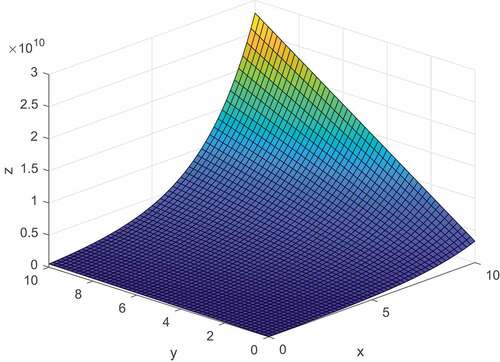
In this section, we deal with the surface plot of generalized Humbert-Hermite polynomials by using some particular values of parameters.

If we choose the values of parameters in generalized Humbert-Hermite polynomials as $\mathit{a}=5,\mathit{b}=6,\mathit{c}=7,\mathit{d}=5,\mathit{e}=3,\mathit{g}=3,\mathit{\mu }=-4,\mathit{\gamma }=4,\mathit{\ell }=0.1,\mathit{m}=8$ and r = 8 in (2.1(2.1) $\begin{array}{l}[\mathit{a}-(\mathit{b\alpha }+\mathit{c\beta })\mathit{\ell }+\mathit{d}{\ell }^m(\mathit{e\alpha \beta }-1{)}^g{]}^{-\mathit{\mu }}{e}^{\gamma (\alpha +\beta )\ell -(\alpha \beta +1){\ell }^r}\\ =\sum _{\mathit{\eta }=0}^{\mathrm{\infty }}{\mathit{ }}_{\mathcal{H}}{\mathcal{Q}}_{\eta ,m,\mu ,r,\gamma }^{a,b,c,d,e,g}(\mathit{\alpha },\mathit{\beta }){\ell }^{\mathit{\eta }},\end{array}$(2.1) ), then we have got following surface representation (see Figure 1) of generalized Humbert-Hermite polynomials. By choosing $\mathit{a}=1,\mathit{b}=2,\mathit{c}=2,\mathit{d}=5,\mathit{e}=2,\mathit{g}=1,\mathit{\mu }=-4,\mathit{\gamma }=4,\mathit{\ell }=0.1,\mathit{m}=8$ and r = 8 in (2.1(2.1) $\begin{array}{l}[\mathit{a}-(\mathit{b\alpha }+\mathit{c\beta })\mathit{\ell }+\mathit{d}{\ell }^m(\mathit{e\alpha \beta }-1{)}^g{]}^{-\mathit{\mu }}{e}^{\gamma (\alpha +\beta )\ell -(\alpha \beta +1){\ell }^r}\\ =\sum _{\mathit{\eta }=0}^{\mathrm{\infty }}{\mathit{ }}_{\mathcal{H}}{\mathcal{Q}}_{\eta ,m,\mu ,r,\gamma }^{a,b,c,d,e,g}(\mathit{\alpha },\mathit{\beta }){\ell }^{\mathit{\eta }},\end{array}$(2.1) ) then we got the surface representation (see Figure 2) of generalized Humbert Hermite polynomials given by Khan & Pathan, (2021).

Figure 1. ${\mathcal{Q}}_{\eta ,8,-4,8,4}^{5,6,7,5,3,3}\left(\mathit{\alpha },\mathit{\beta }\right)$

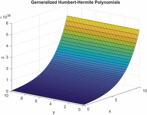
Figure 2. ${\mathcal{Q}}_{\eta ,8,-4,8,4}^{1,2,2,5,2,1}\left(\mathit{\alpha },\mathit{\beta }\right)$

4. Conclusions

The theory of multidimensional or multi-index special functions is a very relevant field of investigation to simplify a wide range of operational relations. It has also been shown that Hermite polynomials play a fundamental role in the extension of the classical special functions to the multidimensional case. In this article, we discuss a new class of generalized Humbert-Hermite polynomials and related special cases for the particular values of the parameters. We have used the generating function (2.1(2.1) $\begin{array}{l}[\mathit{a}-(\mathit{b\alpha }+\mathit{c\beta })\mathit{\ell }+\mathit{d}{\ell }^m(\mathit{e\alpha \beta }-1{)}^g{]}^{-\mathit{\mu }}{e}^{\gamma (\alpha +\beta )\ell -(\alpha \beta +1){\ell }^r}\\ =\sum _{\mathit{\eta }=0}^{\mathrm{\infty }}{\mathit{ }}_{\mathcal{H}}{\mathcal{Q}}_{\eta ,m,\mu ,r,\gamma }^{a,b,c,d,e,g}(\mathit{\alpha },\mathit{\beta }){\ell }^{\mathit{\eta }},\end{array}$(2.1) ) to study their properties and related results. We have also shown their graphical representation by taking the value of unknown parameters in (2.1(2.1) $\begin{array}{l}[\mathit{a}-(\mathit{b\alpha }+\mathit{c\beta })\mathit{\ell }+\mathit{d}{\ell }^m(\mathit{e\alpha \beta }-1{)}^g{]}^{-\mathit{\mu }}{e}^{\gamma (\alpha +\beta )\ell -(\alpha \beta +1){\ell }^r}\\ =\sum _{\mathit{\eta }=0}^{\mathrm{\infty }}{\mathit{ }}_{\mathcal{H}}{\mathcal{Q}}_{\eta ,m,\mu ,r,\gamma }^{a,b,c,d,e,g}(\mathit{\alpha },\mathit{\beta }){\ell }^{\mathit{\eta }},\end{array}$(2.1) ). Using our result (2.1(2.1) $\begin{array}{l}[\mathit{a}-(\mathit{b\alpha }+\mathit{c\beta })\mathit{\ell }+\mathit{d}{\ell }^m(\mathit{e\alpha \beta }-1{)}^g{]}^{-\mathit{\mu }}{e}^{\gamma (\alpha +\beta )\ell -(\alpha \beta +1){\ell }^r}\\ =\sum _{\mathit{\eta }=0}^{\mathrm{\infty }}{\mathit{ }}_{\mathcal{H}}{\mathcal{Q}}_{\eta ,m,\mu ,r,\gamma }^{a,b,c,d,e,g}(\mathit{\alpha },\mathit{\beta }){\ell }^{\mathit{\eta }},\end{array}$(2.1) ) to generalise the well-known class of Gegenbauer, Humbert, Legendre, Chebycheff, Pincherle, Horadam, Kinnsy, Horadam-Pethe, Djordjevi’c, Gould, Milovanovi’c and Djordjevi’c, Pathan and Khan polynomials.

Disclosure statement

No potential conflict of interest was reported by the authors.

Additional information

Notes on contributors

Nabiullah Khan

Nabiullah Khan is a Professor at the Department of Applied Mathematics, Faculty of Engineering and Technology, Aligarh Muslim University, Aligarh. His research interest includes applicable analysis, Special functions especially generating functions and integral transform. He completed his M.Phil and Ph.D. in the years 1998 and 2002 from Aligarh Muslim University. He has more than 100 research article in reputed national and international journals.

Mohammad Iqbal Khan

Mohammad Iqbal Khan is pursuing Ph.D from Department of Applied Mathematics, Faculty of Engineering and Technology at Aligarh Muslim University, Aligarh.

Saddam Husain

Saddam Husain is submitted their Ph.D thesis under the supervision of Prof. Nabiullah Khan at the Department of Applied Mathematics, Faculty of Engineering and Technology at Aligarh Muslim University, Aligarh. His research interest includes applicable analysis, Special functions especially generating functions and integral transform. He has published 14 research article and 8 are communicated in national and international SCI and Scopus journals.

Mohd Asif Shah

Mohd Asif Shah is associated professor at Department of Economics, Kebri Dehar University, Kebri Dehar, Ethiopia. He has published more than 100 research article in national and international reputed journals.

References

- Andrews, L. C. (1985). Special functions for engineers and applied mathematicians. MacMillan.
- Batahan, R. S., & Shehata, A. (2014). Hermite-Chebyshev polynomials with their generalization form. Journal of Mathematical Sciences: Advances and Applications, 29, 47–59.
- Bell, E. T. (1934). Exponential polynomials. Annals of Mathematics, 35(2), 258–277. https://doi.org/10.2307/1968431
- Choi, J., Khan, N., Usman, T., & Aman, M. (2019). Certain unified polynomials. Integral Transforms and Special Functions, 30(1), 28–40. https://doi.org/10.1080/10652469.2018.1534847
- Dattoli, G., Chiccoli, C., Lorenzutta, S., Maino, G., & Torre, A. (1993). Generalized Bessel functions and generalized Hermite polynomials. Journal of Mathematical Analysis and Applications, 178(2), 509–516. https://doi.org/10.1006/jmaa.1993.1321
- Dattoli, G., Lorenzutta, S., & Cesarano, C. (1999). Finite sums and generalized forms of Bernoulli polynomials. Rendiconti di Mathematica, 19, 385–391.
- Dattoli, G., Lorenzutta, S., Maino, G., Torre, A., & Cesarano, C. (1996). Generalized Hermite polynomials and supergaussian forms. Journal of Mathematical Analysis and Applications, 203(3), 597–609. https://doi.org/10.1006/jmaa.1996.0399
- Dattoli, G., Torre, A., & Lorenzutta, S. (1999). Operational identities and properties of ordinary and generalized special functions. Journal of Mathematical Analysis and Applications, 236(2), 399–414.
- Dave, C. K. (1978). Another generalization of Gegenbauer polynomials. Journal of the Indian Academy of Mathematics, 1(2), 42–45.
- Djordjevic, G. B. A generalization of Gegenbauer polynomial with two variables. Indian Journal of Pure Applied Mathematics.
- Djordjevic, G. B., & Milovanovic, G. V. (2014). Special classes of polynomials. University of Nis, Faculty of Technology Leskovac.
- Gould, H. W. (1965). Inverse series relations and other expansions involving Humbert polynomials. Duke Mathematical Journal, 32(4), 697–711. https://doi.org/10.1215/S0012-7094-65-03275-8
- Guan, H., Khan, W. A., & Kızılateş, C. (2023). On generalized bivariate (p, q)-bernoulli-fibonacci polynomials and generalized bivariate (p, q)-bernoulli-lucas polynomials. Symmetry, 15(4), 943. https://doi.org/10.3390/sym15040943
- Horadam, A. F. (1985). Gegenbauer polynomials revisited. Fibonacci Quarterly, 23(4), 294–299.
- Horadam, A. F., & Pethe, S. (1981). Polynomials associated with Gegenbauer polynomials. Fibonacci Quarterly, 19(5), 393–398.
- Khan, W. A. (2019). Certain results for the Hermite and Chebyshev polynomials of 2-variables. Annals of Communication in Mathematics, 2(2), 84–90.
- Khan, N., Aman, M., Usman, T., & Choi, J. (2020). Legendre-Gould Hopper-based Sheffer polynomials and operational methods. Symmetry, 12(12), 2051. https://doi.org/10.3390/sym12122051
- Khan, N., & Husain, S. (2021). Analysis of Bell based Euler polynomials and their application. International Journal of Applied and Computational Mathematics, 7(5), 195. https://doi.org/10.1007/s40819-021-01127-x
- Khan, N., Husain, S. (2022). Certain study of generalized Apostol-Bernoulli poly-daehee polynomials and its properties. Indian Journal of Mathematics.
- Khan, N., Husain, S., Usman, T., & Araci, S. (2023). A new family of Apostol-Genocchi polynomials associated with their certain identities. Applied Mathematics in Science and Engineering, 31(1), 1–19. https://doi.org/10.1080/27690911.2022.2155641
- Khan, W. A., & Pathan, M. A. (2021). On a class of Humbert-Hermite polynomials, December 2021. Novi Sad Journal of Mathematics, 51(1), 1–11. https://doi.org/10.30755/NSJOM.05832
- Milovanovic, G. V., & Djordjevic, G. B. (1987). On some properties of Humbert’s polynomials. Fibonacci Quarterly, 25(4), 356–360.
- Milovanovic, G. V., & Djordjevic, G. B. (1991). On some properties of Humbert’s polynomials II. Facta Universitatis Series: Mathematics and Informatics, 6, 23–30.
- Pathan, M. A., & Khan, M. A. (1997). On polynomials associated with Humbert’s polynomials. Publications de l’Institut Mathématique (beograd)(ns), 62(76), 53–62.
- Pathan, M. A., & Khan, N. U. (2015). A unified presentation of a class of generalized Humbert polynomials in two variables. ROMAI Journal, 11(2), 185–199.
- Pathan, M. A., & Khan, W. A. (2022). On a class of generalized Humbert-Hermite polynomials via generalized Fibonacci polynomials. Turkish Journal of Mathematics, 46(3), 929–945. https://doi.org/10.55730/1300-0098.3133
- Rainville, E. D. (1960). Special functions. The Macmillan Company. Reprinted by Chelsea publishing Company, 1971, Bronx, New York.
- Shrestha, N. B. (1977). Polynomial associated with Legendre polynomials. Nepali Mathematics of Science and Reports Triv Universities, 2(1), 1–7.
- Singh, V., Khan, W. A., Sharma, A., Certain properties and their Volterra integral equation associated with the second kind Chebyshev matrix polynomials in two variables, In Frontiers in Industrial and Applied Mathematics: FIAM-2021, Punjab, India, December 21–22 (pp. 49–65). Singapore: Springer Nature Singapore. (2023).
- Sinha, S. K. (1989). On a polynomial associated with Gegenbauer polynomial. Proceedings of the National Academy of Sciences, India Section A, 59(3), 439–455.
- Usman, T., Khan, N., Aman, M., Al-Omari, S., Nonlaopon, K., & Choi, J. (2022). Some generalized properties of poly-daehee numbers and polynomials based on apostol-genocchi polynomials. Mathematics, 10(14), 2502. https://doi.org/10.3390/math10142502
- Usman, T., Khan, N., Aman, M., & Choi, J. (2022). A family of generalized Legendre-based apostol-type polynomials. Axioms, 11(1), 29.
- Zhang, C., Khan, W. A., & Kızılateş, C. (2023). On (p, q)-fibonacci and (p, q)-lucas polynomials associated with changhee numbers and their properties. Symmetry, 15(4), 851. https://doi.org/10.3390/sym15040851