New approach of convergent numerical method for singularly perturbed delay parabolic convection-diffusion problems

ABSTRACT

In this paper, a parameter-uniform convergent numerical scheme is provided for solving singularly perturbed parabolic convection-diffusion differential equations with a large delay. A priori bounds on the exact solution and its derivatives derived by asymptotic analysis of the problem are provided.. The problem is discretized by the Crank-Nicolson method on uniform mesh in time direction and a fitted operator upwind finite difference method on uniform mesh in spatial direction. The fitting factor is derived from the zeroth-order asymptotic expansion of the exact solution and then introduced for the term containing the singular perturbation parameter. The convergence analysis is given for the proposed numerical method using the barrier function approach and the Peano kernel. We proved the scheme is uniformly convergent with first -order in space and second order in time, both independent of the perturbation parameter. Numerical experiments are presented to support the theoretical findings.

KEYWORDS:

• Fitted operator
• convection-diffusion
• boundary layer
• delay differential equations
• Crank-Nicolson
• peano kernel
• zeroth-order expansion

PUBLIC INTEREST STATEMENT

Singularly perturbed delay differential equations arise from many biological, chemical, and physical systems which are characterized by both spatial and temporal variables. In these equations, the highest derivative is multiplied by a small parameter known as perturbation parameter and also involving at least one delay term with respect to time. Classical finite difference numerical methods on uniform mesh for these equations are unstable and fail to give a good accurate result, because of the presence of the perturbation parameter. The present work developed a nonclassical parameter-uniform convergent numerical scheme based on fitted operator approach for solving parabolic convection-diffusion version of these problems.

1. Introduction

A differential equation is said to be a singularly perturbed delay differential equation (SPDDE) if its highest order derivative term is multiplied by a small perturbation parameter and contains at least one delay term.

Types of SPDDEs appear in many branches of science. To mention a few of them, Model of neural networks (Murat, 2006), chemostat (Zhao, 1995), tumor growth (Villasana & Radunskaya, 2003), circadian rhythms (Smolen et al., 2002), epidemiology (Cooke et al., 1999) and the respiratory system are few of them to be mentioned. In these models, the delay can represent gestation times, incubation periods, and transport delays (Govindarao & Mohapatra, 2018). As an illustrative example, the delayed mathematical model of automatically controlled furnace to produce metal sheet is given by the equation (Wu, 1996)

where denotes the distribution of temperature in a metal sheet and ɛ is a perturbation parameter which satisfies Here, v is the velocity of material strip and f represents a distributed temperature source function. Both v and f depend on time-delayed temperature distribution . A fixed delay of length τ is introduced due to the controlling device’s finite speed. In biological modeling (Bansal et al., 2017), the delay describes primary infection, drug therapy, and immune response.

Existing of the perturbation parameter produces large variation of the solution as it tends to zero. A region where this variation occurs is called boundary layer. This steep gradient or unexpectedly large variation results in failure of classical numerical methods. Because of this, there is growing interest (Debela & Duressa, 2020) in the numerical treatment of such differential equations.

A parameter uniform numerical method for singularly perturbed delay partial differential equations has been developed by many authors. Some of them are listed here. (S. Kumar, (2014) designed uniform convergent layer-adapted numerical methods for a class of initial value problems of quasilinear singularly perturbed first-order delay differential equations using the backward Euler scheme and a high-order hybrid scheme, which is a blend of the Trapezoidal scheme and the backward Euler scheme. (S. Kumar & Kumar, (2017) proposed a hybrid finite difference scheme for a singularly parametrized singularly perturbed first-order delay differential problem on Shishkin and Bakhvalov meshes. They have shown that the method is uniformly convergent of order two (up to logarithmic factor). These authors (S. Kumar & Kumar, 2014) also studied a numerical approximation for a singularly perturbed reaction-diffusion differential equation with delay. They employed a hybrid scheme of HODIE type on a generalized Shishkin mesh and proved that the scheme is second order in temporal variable and fourth order in spatial variable. This singularly perturbed reaction-diffusion differential equation with delay equation was studied by (Singh et al., (2018). The authors used a domain decomposition method and showed that the method was uniformly convergent. (Gupta et al., (2018) developed a higher order numerical approximation for singularly differential convection-diffusion equation involving delay and advance parameters. They used a hybrid scheme of modified midpoint upwind type on a piecewise-uniform Shishkin mesh in spatial direction and Euler implicit scheme on uniform mesh in time direction. Their study shows that the scheme is a parameter uniform convergent order two (up to logarithmic factor).

A class of singularly perturbed large delay parabolic partial differential equations of convection–—diffusion were treated numerically. Recently, authors proposed a parameter uniform finite difference scheme to solve these kinds of problems. Some of them used nonstandard numerical methods likeare, second order a robust numerical method by (Negero & Duressa, (2021, 2022), a higher order robust numerical scheme by (Babu & Bansal, (2022), an exponentially fitted operator finite difference method by (Woldaregay et al., (2021), stable finite difference shcemescheme by (Podila & Kumar, (2020) and second order a robust method of line by (Mbroh et al., (2020).

The aforementioned authors used the nonstandard (Mickens, 2005) or fitted mesh methods for either the central or upwind finite difference. Some other parameter-uniform numerical approximation for singularly perturbed problems based on fitted mesh, domain decomposition, and gride equidistribution approach can be found in the works by Rao and Kumar (2012); S. Kumar et al. (2020); S. Kumar et al., (2022); S. Kumar and Kumar (2016); Rao and Kumar (2011) and the reference therein. In this paper, we propose a parametric uniform convergent upwind exponentially fitted scheme by Crank–—Nicolson time discretization and calculateing a fitting factor from zeroth-order asymptotic expansion of the solution. We analyze convergence of the proposed scheme by barrier function approach and Peano kernel. To the best of our knowledge, this is the first nonstandard numerical scheme for the concerned problem that combines Crank–-Nicolson time discretization with the fitted operator upwind finite difference method, where the fitting factor is calculated from zero-order expansion of exact solution of the continuous problem.

The remaining of the paper is structured as follows: In Section 1, continuous problem formulation and its analytic solution and derivative behavior via bounds are discussed. Section 2 describes an upwind exponentially fitted scheme which is developed by calculating the stabilizing fitting factor. Uniformly convergence analysis of the method is discussed in Section 3. In Section 4, numerical experimentation is carried out in order to verify the theoretical result and to illustrate the accuracy of the method. A summary of the main conclusions is given at the last section.

Throughout the paper, haves taken a generic positive constants which are independent of mesh size, mesh point, and perturbation parameter.

In the following sections denote standard supremum norm and is defined as defined on domain Q.

2. Continuous problem

In this section, we present bounds on the solution and its derivative of a model problem under consideration.

2.1. Problem formulation

We consider the following a one-dimensional singularly perturbed delay parabolic convection-diffusion problem:

(1)

where

(2)

is the singular perturbation parameter and τ > 0 is delay parameter.

. where . Functions on and on Γ are sufficiently smooth, bounded functions, and independent of ɛ. In addition . The terminal time T is assumed to be positive integral multiple of delay parameter τ. Under these conditions, the solution of model problem Eq. (1)(1) exhibits boundary layer at x = 1.

2.2. Bounds on the solution and its derivatives

For The existence and uniqueness of the solution of Eq. (1)(1) on the domain Q is guaranteed by Hlder continuity of the problem data with exponent , along with the following compatibility conditions:

(3)

and

(4)

Under these conditions, Eq.(1(1) ) has unique solution (Ansari et al., 2007). To obtain error estimate for the scheme, we require strong regularity conditions for the solution Eqn (1(1) ). To achieve this, we make the assumption that the problem’s data satisfy strong compatibility conditions at the corner points so that .

Lemma 1.

(Maximum Principle).

Assume , such that , for all and for all . Then, , for all

Proof.

Let such that , assume , it is clear that and From extreme value theorem in Calculus we have, and and then from Eq. (1)(1) -Eq. (2)(2) and we have

which is a contradiction to the assumption made . Hence the Lemma.

Lemma 2.

The solution of Eq. (1)(1) satisfies the following estimate:

Proof.

Refer Negero and Duressa (2021).

Lemma 3.

The solution of Eq. (1)(1) satisfies the following bound:

Proof.

Using Lemma 2

Next Lemma gives uniform stability estimate for solution of Eq. (1)(1) .

Lemma 4.

The solution of Eq. (1)(1) satisfies

Proof.

Introduce barrier functions such that

We have

and for all

By using maximum principle, we obtain the required result.

The following theorem shows the bounds and the existence and uniqueness of derivatives of solution for Eq. (1)(1)

Theorem 2.1

The derivatives of the solution of Eq. (1)(1) satisfy

where l and m are non-negative integers.

Proof.

Refer Salama and Al-Amery (2017).

3. Numerical scheme

In this section, we discuss a numerical method which comprises the Crank–-Nicolson finite difference method for temporal derivative and upwind exponential fitting scheme for spatial derivative on uniform mesh.

3.1. Time discretization

We use uniform mesh for the considered time domain with time step size as , where M +1 denote the number of mesh points in time interval . For temporal lag τ, , p +1 is the number of mesh points in time-interval . Recall that for some positive integer m. Crank–-Nicolson finite difference scheme is used for time derivative discretization for problem Eq. (1)(1) and we obtain semi-discretized problem

(5)

where , , whereas denote the semi-discretized approximation of the exact solution at time level.

Lemma 5.

(Semi-discrete maximum principle).

For sufficiently smooth function , if and for all , then for all .

Proof.

Assume be such that and . From calculus property, we have and . Thus, , which contradict to the hypothesis made . Therefore, for all .

Now consider local and global error estimate. The local truncation error of Eq. (5)(5) at time level is given by , where is solution of the following equation:

This error measures the contribution of each time step to the global error of the time semidiscretization, which is defined, at the instant t_i; as ,

Lemma 6.

If for , in the time direction local error estimate satisfy

(6)

and global error estimate satisfy

(7)

Proof.

By applying Taylor series approximation, we obtain the following central difference formula.

(8)

where After some manipulation, we get,

Now from the definition of , we have

where Since , it is solution of the boundary value problem

(9)

Using Lemma 5 for the operator , we obtain local error estimate

Global error estimate at i time level is

The next lemma provides a bound for the derivatives of solution of Eq. (5)(5) .

Lemma 7.

The solution of Eq. (5)(5) satisfiesy

(10)

Proof.

Refer Bansal and Sharma (2017).

3.2. Spatial discretization

Consider uniform mesh, , . Let define difference operator on U_j

(11)

To stabilize the discretization method, a general strategy we follow is adding artificial diffusion (or artificial viscosity) for the term containing singular perturbation parameter in the given differential equation. This artificial diffusion is introduced by means of fitting factor σ. Consider two-point boundary value problem

(12)

on , where and . Assume that , and f are arbitrary smooth. Asymptotic solution of Eq. (12)(12) is exist and is unique (O’Malley, 1991; O’Malley, 1974,; (Ejere et al., 2022) and expressed as

(13)

where . u_i represents the smooth outer solution and R_i is boundary layer correction which decay to zero as the stretch fast variable tends to infinity. Further, R_i satisfiesy the homogeneous equation of Eq (12)(12) . Asymptotic expansion of zeros order for Eq. (13)(13) is given by , where u₀ is the reduced solution (by making ɛ = 0) at Eq. (12)(12) . R₀ is right boundary layer correction. R₀ satisfiesy the homogeneous differential equation

Solving this equation, we get , so that . The constant A is to be determined. Then,

(14)

Using given boundary condition, we obtain . Now Eq. (14)(14) becomes

(15)

For detail, a reader can refer O’Malley (1991). Compute Eq. (15)(15) in a limit case at as . Let

(16)

Now let us determine the fitting factor σ. Since our scheme is fitted operator upwind finite difference for spatial derivative, then Eq. (12)(12) becomes

(17)

(18)

Computing this expression in both sides as h → 0 using Eq. (16(16) ) , we get

(19)

As a necessary condition for uniform convergence, Roos et al. (2008) take

(20)

which is Bernoulli function form. Numerical methods, like above, whose coefficients involve exponential function are known collectively as exponentially fitted scheme (Roos et al.,(2008). Hence, σ is called exponentially fitted factor. Exponentially fitting is widely used in semiconductor device modeling problem. By applying σ with upwind finite difference for first-order spatial derivative of problem Eq. (5)(5) , we achieve full discretization scheme as

(21)

where Rearranging the terms in Eq. (21)(21) , we get the following system of equations

(22)

The coefficients are given by

(23)

(24)

Lemma 8.

(Discrete Maximum principle).

Let be any mesh on Q. Assume that the mesh function satisfies and . Then, , for all , implies on

Proof.

Let k be such that and suppose that . It is clear that . Therefore,

which is false. Hence, and for all j,

4. Convergence analysis

In this section, we prove convergence of the developed scheme through stability and consistency.

4.1. Stability

The following lemma provides existence and uniqueness of discrete solution.

Lemma 9.

(Discrete Comparison Principle).

The difference operator , with and specified, has a solution. If , and , then

Proof.

The matrix associated with operator is the size of with and for It is easily to observe that the coefficient matrix is diagonally dominant. Thus, it satisfies the property of M matrix. For detail, refer Kellogg and Tsan (1978).

Definition 1.

Roos et al. (2008) A discrete problem is stable in the discrete maximum norm if there exists a constant K (the stability constant) that is independent of h, such that

(25)

for all mesh functions U_h.

The following Lemma enables us to get a bound for .

Lemma 10.

Let . Then, , where C > 0 does not depend on

Proof.

Lemma 11.

The upwind scheme Eq. (22)(22) is uniformly stable with respect to the perturbation parameter

(26)

with stability constant C₁, which is independent of ɛ and

Proof.

Introduce barrier functions ,

By applying the discrete maximum principle on , we obtain Eq. (26)(26) . In view of Definition 1 and Lemma 10, the stability constant is , whereλ is the lower bound of

Lemma 12.

If be any mesh function so that , then

Proof.

Let . Consider two mesh functions defined by . Clearly and

The use of discrete maximum principle, gives the required result.

4.2. Consistency

We now consider truncation error associated with the difference operator . For simplicity, let . Define truncation error at some fixed time level as

(27)

Theorem 4.1

Assume are sufficiently smooth so that . Then the numerical solution of Eq. (22)(22) satisfies

(28)

Proof.

From Peano kernel theorem as in Kellogg and Tsan (1978) for smooth function u(x), we obtain the formulas

(29)

(30)

(31)

(32)

(33)

(34)

and thus,

(35)

(36)

We are doing at some fixed time level, say at i +1, so for convenience we omit it in the calculation (i.e. it appear as superscript).

(37)

Using Eq. (32)(32) and Eq. (36)(36) , the equation Eq. (37)(37) becomes

(38)

From differential equation Eq. (12)(12) ,

and Eq. (31)(31) , we have

(39)

Using Eqs. (37)(37) , (38(38) ), and (39(39) ) with some manipulations, we have

(40)

Dividing both sides by , and again with some manipulations, we can get the following. Recall

(41)

From MacLaurin expansion , we have for . Thus,

This implies

(42)

Using Eq. (41)(41) and Eq. (42)(42) , we have

(43)

That is

(44)

(45)

Using Lemma 7

(46)

(47)

Lemma 13.

For all positive integer k on a fixed mesh, the following is true

Proof.

Consider partition of the interval . Clearly, and . For , we have

Let Then, , as ɛ → 0. Repeated application of L’Hospital’s rule gives

Thus, the proof is completed.

Theorem 4.2

The upwind scheme Eq. (22)(22) is first order uniformly convergent in the discrete maximum norm

(48)

Proof.

Use Lemmas 12, 13, and Theorem 4.1.

The following theorem gives the main result of the paper for ɛ-uniform convergence of the numerical solution.

Theorem 4.3

Let u and U are the continuous and numerical solution of Eq. (1)(1) and Eq. (22)(22) , respectively. We get the following estimate:

(49)

Proof.

Combine error estimate done for temporal and spatial.

5. Numerical result

In this section, to validate the theoretical result, we do numerical experiment on two test problems on rectangular uniform mesh .

Example 1.

Consider the following singularly perturbed time-delay parabolic convection-diffusion problem (Gowrisankar & Natesan, 2017)

Example 2.

Consider singularly perturbed delay parabolic initial boundary value problem (D. Kumar & Kumari, 2019):

Since exact solutions of the test problems are not known, so to find maximum point-wise error, we use double mesh principle. The maximum point-wise error and the corresponding order of convergence are computed as

The uniform error and the corresponding uniform order of convergence are calculated as

Figure 1 and Figure 2 show the numerical solution of problems in Examples 1 and 2, respectively, with specified values of ɛ given there. From both figures, we observe the existence of a boundary layer in the neighbor of x = 1 and how the boundary layer behaves as ɛ → 0. Thus, as ɛ → 0, visibility of the boundary layer increases. Tables 1 and 2 give maximum point-wise error, and the corresponding order of convergence for Examples 1 and 2, respectively, for different values of . From these tables we observe that, as ɛ gets smaller and smaller, the maximum point-wise error becomes almost the same. This means the proposed method is not affected by ɛ in calculating the numerical solution of given examples; it is ɛ-uniform and stable. One also observes that, when the given mesh is refined, maximum point-wise error decreases. The last row gives the order of convergence as illustrative for smaller value of ɛ. Figure. 3 displays the plot of N versus maximum point-wise errors in log-log scale for both Examples 1 and 2. As N increases, the monotonically decreasing behavior of the maximum point-wise errors can be observed from the Figure 3. This figure also confirms that the proposed method is almost first-order accurate and is ɛ –- uniformly convergent and stable. The second-order convergence of the temporal discretization is depicted in Table 3. To confirm that the proposed method works better than Gowrisankar and Natesan (2017) and Podila and Kumar (2020), we compared our result in Table 4 for Example 1.

Figure 1. Numerical solution of example 1, with .

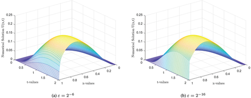
Figure 2. Numerical solution of example 2, with .

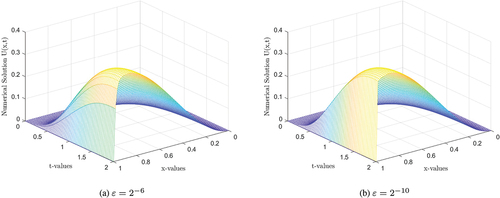
Figure 3. Log-log plot of maximum point-wise error 3a for Example 1 and 3b for Example 2.

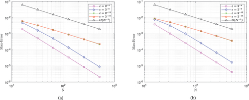
Table 1. Example 1: Maximum point-wise error of the numerical solution

2^0	2.9090	9.8737	2.1590	5.3272	1.3244	3.3037e-07
2^−2	7.6105	1.7672	4.5283	1.1344	2.8292	7.0758e-07
2^−4	1.8970	5.2094	1.3386	3.3689	8.4366	2.1100
2^−6	4.8505	1.6428	5.1394	1.3746	3.4989	8.7869
2^−8	5.9178	3.2448	1.4222	4.6993	1.3173	3.4968
2^−10	5.9184	3.2992	1.7383	8.7450	3.7411	1.2166
2^−12	5.9184	3.2992	1.7387	8.9106	4.5079	2.2243
2^−14	5.9184	3.2992	1.7387	8.9106	4.5088	2.2678
2^−16	5.9184	3.2992	1.7387	8.9106	4.5088	2.2678
2^−18	5.9184	3.2992	1.7387	8.9106	4.5088	2.2678
2^−20	5.9184	3.2992	1.7387	8.9106	4.5088	2.2678
	5.9184	3.2992	1.7387	8.9106	4.5088	2.2678
	0.843090968	0.92410721	0.964414543	0.982779063	0.991450104

Table 2. Example 2: Maximum point-wise error of the numerical solution when N = M

2^0	3.2597	8.1538	2.0398	5.1000	1.2751	3.1877e-07
2^−2	1.1194	2.8266	7.0814	1.7715	4.4294	1.1074
2^−4	3.8077	1.0301	2.6297	6.6093	1.6546	4.1380
2^−6	7.8296	3.2001	9.8362	2.6170	6.6503	1.6695
2^−8	8.7350	5.0115	2.1091	8.1923	2.4829	6.5759
2^−10	8.7361	5.1124	2.7585	1.4012	5.7951	2.0602
2^−12	8.7361	5.1124	2.7590	1.4328	7.2983	3.6013
2^−14	8.7361	5.1124	2.7590	1.4328	7.2999	3.6844
2^−16	8.7361	5.1124	2.7590	1.4328	7.2999	3.6844
2^−18	8.7361	5.1124	2.7590	1.4328	7.2999	3.6844
2^−20	8.7361	5.1124	2.7590	1.4328	7.2999	3.6844
	8.7361	5.1124	2.7590	1.4328	7.2999	3.6844
	0.772988652	0.889855262	0.945308214	0.972888636	0.986447004

Table 3. Maximum absolute error and rate of convergence of the scheme in temporal direction

	Example 1				Example 2
	N = 16	64	256		N = 16	64	256
	M = 10	20	40		M = 16	32	64
2^−10	5.9184	1.7386	3.7644		8.7361	2.8319	6.0301
	1.7673	2.2075			1.6252	2.2315
2^−12	5.9184	1.7389	4.5281		8.7361	2.8324	7.5551
	1.7670	1.9412			1.6249	1.9065
2^−14	5.9184	1.7389	4.5290		8.7361	2.8324	7.5569
	1.7670	1.9409			1.6249	1.9062
2^−16	5.9184	1.7389	4.5290		8.7361	2.8324	7.5569
	1.7670	1.9409			1.6249	1.9062
2^−18	5.9184	1.7389	4.5290		8.7361	2.8324	7.5569
	1.7670	1.9409			1.6249	1.9062
2^−20	5.9184	1.7389	4.5290		8.7361	2.8324	7.5569
	1.7670	1.9409			1.6249	1.9062
	5.9184	1.7389	4.5290		8.7361	2.8324	7.5569
	1.7670	1.9409			1.6249	1.9062

Table 4. Comparison of uniform error and order of convergence for Example 1 at with Gowrisankar and Natesan (2017)

Method	N = 16	32	64	128	256	512
	M = 10	20	40	80	160	320
Proposed method
	5.9184	3.2992	1.7387	8.9106	4.5079	2.2243
	0.8431	0.9241	0.9644	0.9831	1.0191
Method byin(Gowrisankar & Natesan,(2017)
	9.7396e-02	7.0964e-02	4.6232e-02	2.8377e-02	1.6719e-02	9.5805
	0.4568	0.6182	0.7042	0.7632	0.8033
Method byin(Podila & Kumar,(2020)
	7.4252	4.0993	2.1528	1.1033	5.5835
	0.8571	0.9292	0.9644	0.9826

6. Conclusion

In this paper, we have proposed a fitted operator numerical approach to solve singularly perturbed large delay parabolic conviction-diffusion problem with Dirichlet boundary conditions. The behavior of a continuous solution is examined via the bounds of the solution and its derivative. The temporal and spatial domains are discretized with uniform mesh. The numerical scheme consists of the Crank–-Nicolson scheme for time derivative and the upwind scheme for first-order spatial derivative. Due to the presence of a perturbation parameter, the problem exhibits right side boundary layer. The fitting factor is introduced for controlling variation of solution in the boundary layer region.; The perturbation parameter ɛ affecting the highest derivative is replaced by the fitting factor. The convergence of the proposed scheme is discussed and investigated theoretically via stability and consistency. The stability of the scheme is proved by using the technique of solution bound by constructing barrier functions. The consistency of the scheme is proved by the truncation error estimate in integral form. We have developed a parameter-uniform error bound for the proposed method, which is second order in time and first order in spatial, ). The theoretical results are validated by two test examples. As a practical interest, for our future work, we will apply the scheme for nonlinear singularly perturbed parabolic convection–—diffusion problems with degenerate coefficients. An interested researcher can also extend the proposed method for other meaningful mathematical models with large time delay.

Acknowledgements

The authors express their thanks to the anonymous reviewers for valuable comments and suggestions which improved the paper.

Disclosure statement

No potential conflict of interest was reported by the author(s).

Additional information

Funding

This research received no specific funding from public, private, or non-profit funding agencies.

Notes on contributors

Zerihun Ibrahim Hassen

Zerihun Ibrahim Hassen is a PhD candidate at the Department of Mathematics, College of Natural and Computational Sciences, Arba Minch University, Ethiopia. His research interest includes development of numerical methods for the delay partial differential equation and applied mathematics.

Gemechis File Duressa

Gemechis File Duressa holds an M.Sc. from Addis Ababa University in Ethiopia and a Ph.D. from the National Institute of Technology in Warangal, India. He is currently employed as a full professor of mathematics and Director of the School of graduate studies at Jimma University in Ethiopia. So far, he published more than 164 research articles in national and international reputable journals. His research interests span on the areas of numerical solutions of differential equations, mainly on singularly perturbed ordinary and partial differential equations. He made numerous contributions in serving as a reviewer, assistant editor and editor for various national and international Journals.

References

- Ansari, A., Bakr, S., & Shishkin, G. (2007). A parameter-robust finite difference method for singularly perturbed delay parabolic partial differential equations. Journal of Computational and Applied Mathematics, 205(1), 552–566. https://doi.org/10.1016/j.cam.2006.05.032
- Babu, G., & Bansal, K. (2022). A high order robust numerical scheme for singularly perturbed delay parabolic convection diffusion problems. Journal of Applied Mathematics and Computing, 68(1), 363–389. https://doi.org/10.1007/s12190-021-01512-1
- Bansal, K., Rai, P., & Sharma, K. K. (2017). Numerical treatment for the class of time dependent singularly perturbed parabolic problems with general shift arguments. Differential Equations and Dynamical Systems, 25(2), 327–346. https://doi.org/10.1007/s12591-015-0265-7
- Bansal, K., & Sharma, K. K. (2017). Parameter uniform numerical scheme for time dependent singularly perturbed convection-diffusion-reaction problems with general shift arguments. Numerical Algorithms, 75(1), 113–145. https://doi.org/10.1007/s11075-016-0199-3
- Cooke, K., Van den Driessche, P., & Zou, X. (1999). Interaction of maturation delay and nonlinear birth in population and epidemic models. Journal of Mathematical Biology, 39(4), 332–352. https://doi.org/10.1007/s002850050194
- Debela, H. G., & Duressa, G. F. (2020). Accelerated fitted operator finite difference method for singularly perturbed delay differential equations with non-local boundary condition. Journal of the Egyptian Mathematical Society, 28(1), 1–16. https://doi.org/10.1186/s42787-020-00076-6
- Ejere, A. H., Duressa, G. F., Woldaregay, M. M., Dinka, T. G., & Migorski, S. (2022). An exponentially fitted numerical scheme via domain decomposition for solving singularly perturbed differential equations with large negative shift. Journal of Mathematics, 2022, 1–13. https://doi.org/10.1155/2022/7974134
- Govindarao, L., & Mohapatra, J. (2018). A second order numerical method for singularly perturbed delay parabolic partial differential equation. Engineering Computations, 36(2), 420–444. https://doi.org/10.1108/EC-08-2018-0337
- Gowrisankar, S., & Natesan, S. (2017). Ɛ-uniformly convergent numerical scheme for singularly perturbed delay parabolic partial differential equations. International Journal of Computer Mathematics, 94(5), 902–921. https://doi.org/10.1080/00207160.2016.1154948
- Gupta, V., Kumar, M., & Kumar, S. (2018). Higher order numerical approximation for time dependent singularly perturbed differential-difference convection-diffusion equations. Numerical Methods for Partial Differential Equations, 34(1), 357–380. https://doi.org/10.1002/num.22203
- Kellogg, R. B., & Tsan, A. (1978). Analysis of some difference approximations for a singular perturbation problem without turning points. Mathematics of Computation, 32(144), 1025–1039. https://doi.org/10.1090/S0025-5718-1978-0483484-9
- Kumar, S. (2014). Layer-adapted methods for quasilinear singularly perturbed delay differential problems. Applied Mathematics and Computation, 233, 214–221. https://doi.org/10.1016/j.amc.2014.02.002
- Kumar, S., & Kumar, M. (2014). High order parameter-uniform discretization for singularly perturbed parabolic partial differential equations with time delay. Computers & Mathematics with Applications, 68(10), 1355–1367. https://doi.org/10.1016/j.camwa.2014.09.004
- Kumar, S., & Kumar, M. (2016). Analysis of some numerical methods on layer adapted meshes for singularly perturbed quasilinear systems. Numerical Algorithms, 71(1), 139–150. https://doi.org/10.1007/s11075-015-9989-2
- Kumar, S., & Kumar, M. (2017). A second order uniformly convergent numerical scheme for parameterized singularly perturbed delay differential problems. Numerical Algorithms, 76(2), 349–360. https://doi.org/10.1007/s11075-016-0258-9
- Kumar, D., & Kumari, P. (2019). A parameter-uniform numerical scheme for the parabolic singularly perturbed initial boundary value problems with large time delay. Journal of Applied Mathematics and Computing, 59(1), 179–206. https://doi.org/10.1007/s12190-018-1174-z
- Kumar, S., Kumar, S.K., & Kumar, M. (2020). A robust numerical method for a two-parameter singularly perturbed time delay parabolic problem. Computational and Applied Mathematics, 39(3), 1–25. https://doi.org/10.1007/s40314-020-01236-1
- Kumar, S., Vigo-Aguiar, J., & Vigo-Aguiar, J. (2022). A parameter-uniform grid equidistribution method for singularly perturbed degenerate parabolic convection–diffusion problems. Journal of Computational and Applied Mathematics, 404, 113273. https://doi.org/10.1016/j.cam.2020.113273
- Mbroh, N. A., Noutchie, S. C. O., & Massoukou, R. Y. M. (2020). A robust method of lines solution for singularly perturbed delay parabolic problem. Alexandria Engineering Journal, 59(4), 2543–2554. https://doi.org/10.1016/j.aej.2020.03.042
- Mickens, R. E. (2005). Advances in the applications of nonstandard finite difference schemes. World Scientific. https://doi.org/10.1142/5884, https://doi.org/10.1142/5884
- Murat, Y. S. (2006). Comparison of fuzzy logic and artificial neural networks approaches in vehicle delay modeling. Transportation Research Part C: Emerging Technologies, 14(5), 316–334. https://doi.org/10.1016/j.trc.2006.08.003
- Negero, N. T., & Duressa, G. F. (2021). A method of line with improved accuracy for singularly perturbed parabolic convection–diffusion problems with large temporal lag. Results in Applied Mathematics, 11, 100174. https://doi.org/10.1016/j.rinam.2021.100174
- Negero, N. T., & Duressa, G. F. (2022). A method of line with improved accuracy for singularly perturbed parabolic convection–diffusion problems with large temporal lag. Tamkang Journal of Mathematics, 11, 100174. https://doi.org/10.1016/j.rinam.2021.100174/
- O’Malley, R. E., Jr. (1974). Introduction to singular perturbations. volume 14. applied mathematics and mechanics. (Tech. Rep). New York Univ Ny Courant Inst of Mathematical Sciences.
- O’Malley, R. E. (1991). Singular perturbation methods for ordinary differential equations (Vol. 89). Springer. https://doi.org/10.1007/978-1-4612-0977-5
- Podila, P. C., & Kumar, K. (2020). A new stable finite difference scheme and its convergence for time-delayed singularly perturbed parabolic PDEs. Computational and Applied Mathematics, 39(3), 1–16. https://doi.org/10.1007/s40314-020-01170-2
- Rao, S. C. S., & Kumar, S. (2011). An almost fourth order uniformly convergent domain decomposition method for a coupled system of singularly perturbed reaction–diffusion equations. Journal of Computational and Applied Mathematics, 235(11), 3342–3354. https://doi.org/10.1016/j.cam.2011.01.047
- Rao, S. C. S., & Kumar, S. (2012). Second order global uniformly convergent numerical method for a coupled system of singularly perturbed initial value problems. Applied Mathematics and Computation, 219(8), 3740–3753. https://doi.org/10.1016/j.amc.2012.09.075
- Roos, H. G., Stynes, M., & Tobiska, L. (2008). Robust numerical methods for singularly perturbed differential equations: Convection-diffusion-reaction and flow problems (Vol. 24). Springer Science & Business Media. https://doi.org/10.1007/978-3-540-34467-4
- Salama, A., & Al-Amery, D. (2017). A higher order uniformly convergent method for singularly perturbed delay parabolic partial differential equations. International Journal of Computer Mathematics, 94(12), 2520–2546. https://doi.org/10.1080/00207160.2017.1284317
- Singh, J., Kumar, S., & Kumar, M. (2018). A domain decomposition method for solving singularly perturbed parabolic reaction-diffusion problems with time delay. Numerical Methods for Partial Differential Equations, 34(5), 1849–1866. https://doi.org/10.1002/num.22256
- Smolen, P., Baxter, D. A., & Byrne, J. H. (2002). A reduced model clarifies the role of feedback loops and time delays in the drosophila circadian oscillator. Biophysical Journal, 83(5), 2349–2359. https://doi.org/10.1016/S0006-34950275249-1
- Villasana, M., & Radunskaya, A. (2003). A delay differential equation model for tumor growth. Journal of Mathematical Biology, 47(3), 270–294. https://doi.org/10.1007/s00285-003-0211-0
- Woldaregay, M. M., Aniley, W. T., Duressa, G. F., & Macias Diaz, J. E. (2021). Novel numerical scheme for singularly perturbed time delay convection-diffusion equation. Advances in Mathematical Physics, 2021, 1–13. https://doi.org/10.1155/2021/6641236
- Wu, J. (1996). Theory and applications of partial functional differential equations. Vol. 119. Springer Science & Business Media. https://doi.org/10.1007/978-1-4612-4050-1
- Zhao, T. (1995). Global periodic-solutions for a differential delay system modeling a microbial population in the chemostat. Journal of Mathematical Analysis and Applications, 193(1), 329–352. https://doi.org/10.1006/jmaa.1995.1239