Fitted numerical scheme for singularly perturbed parabolic differential- difference with time lag

ABSTRACT

This paper deals with the numerical treatment of a singularly perturbed parabolic differential-difference equation with time delay. Taylor’s series expansion is employed to approximate the terms with shift arguments in both spatial and time directions. The resulting problem is discretized using the implicit Euler method and fitted exponential cubic spline methods for time and space variables, respectively. The stability and uniform convergence of the proposed scheme are investigated. The scheme is proved to be uniformly convergent with the order of convergence $O(\mathrm{\Delta }t+{\ell }^2)$. A model test problem is considered to validate the applicability and efficiency of the scheme. It is observed that the proposed scheme provides more accurate results than methods available in the literature.

KEYWORDS:

• Singular perturbation problem
• differential-difference equation
• implicit Euler method
• exponential cubic spline method

MATHEMATICS SUBJECT CLASSIFICATION:

• 35B25
• 35K67
• 65M12

1. Introduction

In this study, we consider the following singularly perturbed parabolic differential-difference equation (SPPDDE) with time delay on the domain $D=G_z\times G_t=(0,1)\times (0,T],\mathrm{\Gamma }={\mathrm{\Gamma }}_l\cup {\mathrm{\Gamma }}_b\cup {\mathrm{\Gamma }}_r$ of the form:

(1.1) $\{\begin{array}{l}\frac{\partial u(z,t)}{\partial t}-\epsilon \frac{{\partial }^{2}u(z,t)}{\partial z^2}+a(z)\frac{\partial u(z,t)}{\partial z}+b(z)u(z-\delta ,t)+c(z)u(z,t)\\ +d(z)u(z-\eta ,t)=-f(z,t)u(z,t-\xi )+g(z,t),(z,t)\in D,\\ u(z,t)={\psi }_b(z,t),(z,t)\in {\mathrm{\Gamma }}_b,\\ u(z,t)={\psi }_l(z,t),\mathrm{\forall }\in {\mathrm{\Gamma }}_l=\{(z,t):-\delta \le z\le 0,t\in {\bar{G}}_t\},\\ u(z,t)={\psi }_r(z,t),\mathrm{\forall }\in {\mathrm{\Gamma }}_r=\{(z,t):1\le z\le 1+\eta ,t\in {\bar{G}}_t\},\end{array}$(1.1)

where ${\mathrm{\Gamma }}_l$ and ${\mathrm{\Gamma }}_r$ are the left and right sides of the rectangular domain D corresponding to z = 0 and z = 1, respectively. ${\mathrm{\Gamma }}_b=[0,1]\times [-\xi ,0]$. $0<\epsilon \ll 1$ is a singular perturbation parameter, η is positive shift (advance) parameter, δ and ξ are negative shift (delay) parameters in space and time direction, respectively, and $\delta ,\eta ,\xi =o(\epsilon ),\delta ,\eta ,\xi >0$. The functions $a(z),b(z),c(z),d(z),f(z),g(z,t),{\psi }_b(z,t),{\psi }_l(z,t)$ and ${\psi }_r(z,t)$ on Γ are assumed to be sufficiently smooth, bounded and independent of ɛ.

The model problem (1.1(1.1) $\{\begin{array}{l}\frac{\partial u(z,t)}{\partial t}-\epsilon \frac{{\partial }^{2}u(z,t)}{\partial z^2}+a(z)\frac{\partial u(z,t)}{\partial z}+b(z)u(z-\delta ,t)+c(z)u(z,t)\\ +d(z)u(z-\eta ,t)=-f(z,t)u(z,t-\xi )+g(z,t),(z,t)\in D,\\ u(z,t)={\psi }_b(z,t),(z,t)\in {\mathrm{\Gamma }}_b,\\ u(z,t)={\psi }_l(z,t),\mathrm{\forall }\in {\mathrm{\Gamma }}_l=\{(z,t):-\delta \le z\le 0,t\in {\bar{G}}_t\},\\ u(z,t)={\psi }_r(z,t),\mathrm{\forall }\in {\mathrm{\Gamma }}_r=\{(z,t):1\le z\le 1+\eta ,t\in {\bar{G}}_t\},\end{array}$(1.1) ) is used to describe the time evolution trajectories of the membrane potential when ξ = 0 (Musila & Lánsk’y, 1991) and used to describe a furnace used to process metal sheets when $\delta =\eta =0$ (Wang, 1963). The dual presence of singular perturbations and shift arguments in both space and time directions in Eq. (1.1)(1.1) $\{\begin{array}{l}\frac{\partial u(z,t)}{\partial t}-\epsilon \frac{{\partial }^{2}u(z,t)}{\partial z^2}+a(z)\frac{\partial u(z,t)}{\partial z}+b(z)u(z-\delta ,t)+c(z)u(z,t)\\ +d(z)u(z-\eta ,t)=-f(z,t)u(z,t-\xi )+g(z,t),(z,t)\in D,\\ u(z,t)={\psi }_b(z,t),(z,t)\in {\mathrm{\Gamma }}_b,\\ u(z,t)={\psi }_l(z,t),\mathrm{\forall }\in {\mathrm{\Gamma }}_l=\{(z,t):-\delta \le z\le 0,t\in {\bar{G}}_t\},\\ u(z,t)={\psi }_r(z,t),\mathrm{\forall }\in {\mathrm{\Gamma }}_r=\{(z,t):1\le z\le 1+\eta ,t\in {\bar{G}}_t\},\end{array}$(1.1) increases the difficulty of obtaining oscillation-free solutions by applying classical numerical methods. To solve such types of equations, one can look for non-classical numerical methods. The most common non-classical competitive computational schemes developed for Eq. (1.1)(1.1) $\{\begin{array}{l}\frac{\partial u(z,t)}{\partial t}-\epsilon \frac{{\partial }^{2}u(z,t)}{\partial z^2}+a(z)\frac{\partial u(z,t)}{\partial z}+b(z)u(z-\delta ,t)+c(z)u(z,t)\\ +d(z)u(z-\eta ,t)=-f(z,t)u(z,t-\xi )+g(z,t),(z,t)\in D,\\ u(z,t)={\psi }_b(z,t),(z,t)\in {\mathrm{\Gamma }}_b,\\ u(z,t)={\psi }_l(z,t),\mathrm{\forall }\in {\mathrm{\Gamma }}_l=\{(z,t):-\delta \le z\le 0,t\in {\bar{G}}_t\},\\ u(z,t)={\psi }_r(z,t),\mathrm{\forall }\in {\mathrm{\Gamma }}_r=\{(z,t):1\le z\le 1+\eta ,t\in {\bar{G}}_t\},\end{array}$(1.1) and related problems are based on the fitted operator and the fitted mesh approach. For the details of these techniques, one can refer (Doolan et al., 1980; Roos et al., 2008; Shishkin & Shishkina, 2008).

Most of the published works to date have concentrated on singularly perturbed parabolic differential equations with either space delay(s) or time delay, but not both. For instance, the authors in (Daba & Duressa, 2021, 2021a, 2021b, 2021c, 2022a, 2022b, 2022c; Kumar, 2018; Nageshwar Rao & Chakravarthy, 2019; Ramesh & Priyanga, 2019) have suggested different computational techniques for singularly perturbed differential equations with delay/and advance parameter(s). In the articles (Govindarao & Mohapatra, 2020; Govindarao et al., 2019, 2019; Gupta et al., 2019; Negero & Duressa, 2022; Sumit et al., 2020), the authors have presented several parameter numerical schemes for singularly perturbed parabolic differential problems with a time lag. Recently, the numerical treatment of coupled systems of multiple scales, a class of singularly perturbed one- and two-dimensional non-smooth data and non-linear problems have been investigated. For example, an a posteriori based convergence analysis for a nonlinear singularly perturbed system of delay differential equations can observe on an adaptive mesh at (Das, 2019). A parameter uniform numerical method is developed for a two-parameter singularly perturbed parabolic partial differential equation with discontinuous convection coefficient and source term in (Chandru et al., 2019). (Saini et al., 2023) have proposed computational cost reduction for a coupled system of multiple-scale reaction-diffusion problems, with mixed-type boundary conditions having boundary layers. (Shiromani et al., 2023) have suggested a higher-order hybrid-numerical approximation for a class of singularly perturbed two-dimensional convection-diffusion elliptic problems with non-smooth convection and source terms. In (Srivastava et al., 2023), Srivastava et al. have introduced a theoretical study of the fractional-order p-Laplacian nonlinear Hadamard type turbulent flow models having the Ulam-Hyers stability.

More recently (Sahu & Mohapatra, 2021), and (Reddy & Mohapatra, 2023) have developed an $\epsilon -$uniform numerical scheme for singularly perturbed differential equations having both mixed shifts in space and delays in time directions. However, as we have seen from the literature survey, very limited competitive numerical methods exist for solving Eq. (1.1)(1.1) $\{\begin{array}{l}\frac{\partial u(z,t)}{\partial t}-\epsilon \frac{{\partial }^{2}u(z,t)}{\partial z^2}+a(z)\frac{\partial u(z,t)}{\partial z}+b(z)u(z-\delta ,t)+c(z)u(z,t)\\ +d(z)u(z-\eta ,t)=-f(z,t)u(z,t-\xi )+g(z,t),(z,t)\in D,\\ u(z,t)={\psi }_b(z,t),(z,t)\in {\mathrm{\Gamma }}_b,\\ u(z,t)={\psi }_l(z,t),\mathrm{\forall }\in {\mathrm{\Gamma }}_l=\{(z,t):-\delta \le z\le 0,t\in {\bar{G}}_t\},\\ u(z,t)={\psi }_r(z,t),\mathrm{\forall }\in {\mathrm{\Gamma }}_r=\{(z,t):1\le z\le 1+\eta ,t\in {\bar{G}}_t\},\end{array}$(1.1) . To minimize the observed gap, in this article, a parameter uniformly convergent numerical scheme is proposed for Eq. (1.1)(1.1) $\{\begin{array}{l}\frac{\partial u(z,t)}{\partial t}-\epsilon \frac{{\partial }^{2}u(z,t)}{\partial z^2}+a(z)\frac{\partial u(z,t)}{\partial z}+b(z)u(z-\delta ,t)+c(z)u(z,t)\\ +d(z)u(z-\eta ,t)=-f(z,t)u(z,t-\xi )+g(z,t),(z,t)\in D,\\ u(z,t)={\psi }_b(z,t),(z,t)\in {\mathrm{\Gamma }}_b,\\ u(z,t)={\psi }_l(z,t),\mathrm{\forall }\in {\mathrm{\Gamma }}_l=\{(z,t):-\delta \le z\le 0,t\in {\bar{G}}_t\},\\ u(z,t)={\psi }_r(z,t),\mathrm{\forall }\in {\mathrm{\Gamma }}_r=\{(z,t):1\le z\le 1+\eta ,t\in {\bar{G}}_t\},\end{array}$(1.1) .

When $\delta ,\eta ,\xi <\epsilon$, the use of Taylor’s series expansion for the terms containing shift arguments is valid (Tian, 2002). Thus, on applying Taylor’s series expansion on the terms with shifts of Eq. (1.1)(1.1) $\{\begin{array}{l}\frac{\partial u(z,t)}{\partial t}-\epsilon \frac{{\partial }^{2}u(z,t)}{\partial z^2}+a(z)\frac{\partial u(z,t)}{\partial z}+b(z)u(z-\delta ,t)+c(z)u(z,t)\\ +d(z)u(z-\eta ,t)=-f(z,t)u(z,t-\xi )+g(z,t),(z,t)\in D,\\ u(z,t)={\psi }_b(z,t),(z,t)\in {\mathrm{\Gamma }}_b,\\ u(z,t)={\psi }_l(z,t),\mathrm{\forall }\in {\mathrm{\Gamma }}_l=\{(z,t):-\delta \le z\le 0,t\in {\bar{G}}_t\},\\ u(z,t)={\psi }_r(z,t),\mathrm{\forall }\in {\mathrm{\Gamma }}_r=\{(z,t):1\le z\le 1+\eta ,t\in {\bar{G}}_t\},\end{array}$(1.1) , we have

(1.2) $\{\begin{array}{l}u(z-\delta ,t)=u(z,t)-\delta u_z(z,t)+\frac{{\delta }^2}{2}{u}_{zz}(z,t)+O({\delta }^3),\\ u(z+\eta ,t)=u(z,t)+\eta u_z(z,t)+\frac{{\eta }^2}{2}{u}_{zz}(z,t)+O({\eta }^3),\\ u(z,t-\xi )=u(z,t)-\xi u_t(z,t)+O({\xi }^2).\end{array}$(1.2)

Substituting Eq. (1.2)(1.2) $\{\begin{array}{l}u(z-\delta ,t)=u(z,t)-\delta u_z(z,t)+\frac{{\delta }^2}{2}{u}_{zz}(z,t)+O({\delta }^3),\\ u(z+\eta ,t)=u(z,t)+\eta u_z(z,t)+\frac{{\eta }^2}{2}{u}_{zz}(z,t)+O({\eta }^3),\\ u(z,t-\xi )=u(z,t)-\xi u_t(z,t)+O({\xi }^2).\end{array}$(1.2) into Eq. (1.1)(1.1) $\{\begin{array}{l}\frac{\partial u(z,t)}{\partial t}-\epsilon \frac{{\partial }^{2}u(z,t)}{\partial z^2}+a(z)\frac{\partial u(z,t)}{\partial z}+b(z)u(z-\delta ,t)+c(z)u(z,t)\\ +d(z)u(z-\eta ,t)=-f(z,t)u(z,t-\xi )+g(z,t),(z,t)\in D,\\ u(z,t)={\psi }_b(z,t),(z,t)\in {\mathrm{\Gamma }}_b,\\ u(z,t)={\psi }_l(z,t),\mathrm{\forall }\in {\mathrm{\Gamma }}_l=\{(z,t):-\delta \le z\le 0,t\in {\bar{G}}_t\},\\ u(z,t)={\psi }_r(z,t),\mathrm{\forall }\in {\mathrm{\Gamma }}_r=\{(z,t):1\le z\le 1+\eta ,t\in {\bar{G}}_t\},\end{array}$(1.1) , we obtain

(1.3) $\{\begin{array}{l}{\text{£}}_{c_{\epsilon }}u(z,t)=F(z)\frac{\partial u(z,t)}{\partial t}-c_{\epsilon }\frac{{\partial }^{2}u(z,t)}{\partial z^2}+p(z)\frac{\partial u(z,t)}{\partial z}\\ +q(z)u(z,t)=g(z,t),(z,t)\in D,\\ u(z,0)={\psi }_b(z,0),z\in {\bar{G}}_z,\\ u(0,t)={\psi }_l(1,t),u(1,t)={\psi }_r(1,t),t\in {\bar{G}}_t,\end{array}$(1.3)

where $F(z)=(1-f(z,t)\xi ),c_{\epsilon }(z)=(\epsilon -b(z)\frac{{\delta }^2}{2}-d(z)\frac{{\eta }^2}{2}),\text{break}p(z)=(a(z)-b(z)\delta +d(z)\eta ),$ $q(z)=(b(z)+c(z)+d(z)\text{break}+f(z,t)).$ The choice of smaller $\delta ,\eta$ and ξ Eqs. (1.1)(1.1) $\{\begin{array}{l}\frac{\partial u(z,t)}{\partial t}-\epsilon \frac{{\partial }^{2}u(z,t)}{\partial z^2}+a(z)\frac{\partial u(z,t)}{\partial z}+b(z)u(z-\delta ,t)+c(z)u(z,t)\\ +d(z)u(z-\eta ,t)=-f(z,t)u(z,t-\xi )+g(z,t),(z,t)\in D,\\ u(z,t)={\psi }_b(z,t),(z,t)\in {\mathrm{\Gamma }}_b,\\ u(z,t)={\psi }_l(z,t),\mathrm{\forall }\in {\mathrm{\Gamma }}_l=\{(z,t):-\delta \le z\le 0,t\in {\bar{G}}_t\},\\ u(z,t)={\psi }_r(z,t),\mathrm{\forall }\in {\mathrm{\Gamma }}_r=\{(z,t):1\le z\le 1+\eta ,t\in {\bar{G}}_t\},\end{array}$(1.1) and (1.3(1.3) $\{\begin{array}{l}{\text{£}}_{c_{\epsilon }}u(z,t)=F(z)\frac{\partial u(z,t)}{\partial t}-c_{\epsilon }\frac{{\partial }^{2}u(z,t)}{\partial z^2}+p(z)\frac{\partial u(z,t)}{\partial z}\\ +q(z)u(z,t)=g(z,t),(z,t)\in D,\\ u(z,0)={\psi }_b(z,0),z\in {\bar{G}}_z,\\ u(0,t)={\psi }_l(1,t),u(1,t)={\psi }_r(1,t),t\in {\bar{G}}_t,\end{array}$(1.3) ) are asymptotically equivalent, because the difference between the two equations is of order of $O({\delta }^3,{\eta }^3,{\xi }^2)$. Assume that $q(z)>\theta >0,c(z)\ge 2{\lambda }_1>0,d(z)>2{\lambda }_2>0,f(z)>2{\lambda }_3>0$, for $z\in G_z$. For $c_{\epsilon }(z)>0$ and $p(z)>2{\gamma }_1>0$, the problem exhibits a layer near z = 1. For $c_{\epsilon }(z)>0$ and $p(z)\le -2{\gamma }_2<0$, the problem exhibits a layer near z = 0. Now, we consider the maximum principle and stability of the solution u in (1.3(1.3) $\{\begin{array}{l}{\text{£}}_{c_{\epsilon }}u(z,t)=F(z)\frac{\partial u(z,t)}{\partial t}-c_{\epsilon }\frac{{\partial }^{2}u(z,t)}{\partial z^2}+p(z)\frac{\partial u(z,t)}{\partial z}\\ +q(z)u(z,t)=g(z,t),(z,t)\in D,\\ u(z,0)={\psi }_b(z,0),z\in {\bar{G}}_z,\\ u(0,t)={\psi }_l(1,t),u(1,t)={\psi }_r(1,t),t\in {\bar{G}}_t,\end{array}$(1.3) ), which is important for the proposed numerical analysis (Das, 2019, Das et al., 2019, Das et al., 2020, Das et al., 2022).

Lemma 1.1.

(Maximum principle) If $u\in C^{2,1}(\bar{D})$, $u{|}_{\partial D}\text{break}\ge 0$ and ${\text{£}}_{\epsilon }u{|}_D\ge 0$, then $u{|}_{\bar{D}}\ge 0$.

Proof.

See (Reddy & Mohapatra, 2023).

An immediate consequence of Lemma 1.1 for the solution of problem (1.3(1.3) $\{\begin{array}{l}{\text{£}}_{c_{\epsilon }}u(z,t)=F(z)\frac{\partial u(z,t)}{\partial t}-c_{\epsilon }\frac{{\partial }^{2}u(z,t)}{\partial z^2}+p(z)\frac{\partial u(z,t)}{\partial z}\\ +q(z)u(z,t)=g(z,t),(z,t)\in D,\\ u(z,0)={\psi }_b(z,0),z\in {\bar{G}}_z,\\ u(0,t)={\psi }_l(1,t),u(1,t)={\psi }_r(1,t),t\in {\bar{G}}_t,\end{array}$(1.3) ) gives the next Lemma 1.2.

Lemma 1.2.

(Continuous stability estimate) Let $u(z,t)$ be the solution of the problem (1.3(1.3) $\{\begin{array}{l}{\text{£}}_{c_{\epsilon }}u(z,t)=F(z)\frac{\partial u(z,t)}{\partial t}-c_{\epsilon }\frac{{\partial }^{2}u(z,t)}{\partial z^2}+p(z)\frac{\partial u(z,t)}{\partial z}\\ +q(z)u(z,t)=g(z,t),(z,t)\in D,\\ u(z,0)={\psi }_b(z,0),z\in {\bar{G}}_z,\\ u(0,t)={\psi }_l(1,t),u(1,t)={\psi }_r(1,t),t\in {\bar{G}}_t,\end{array}$(1.3) ), then we have

$\begin{array}{ll}\Vert u\Vert \le {\theta }^{-1}\Vert g\Vert +& max\{\left|{\psi }_b(z,0)\right|,\\ & max\{\left|{\psi }_l(0,t)\right|,\left|{\psi }_r(1,t)\right|\}\},\end{array}$

where $\Vert .\Vert$ is the $L_{\mathrm{\infty }}$ norm given by $\Vert u\Vert =\underset{(z,t)\in \bar{D}}{max}\text{break}|u(z,t)|.$

Proof.

Let ${\mathrm{\Phi }}^{\pm }(z,t)$ be two barrier functions defined by

$\begin{array}{ll}{\mathrm{\Phi }}^{\pm }(z,t)=& {\theta }^{-1}\Vert g\Vert +max\{\left|{\psi }_b(z,0)\right|,max\{\left|{\psi }_l(0,t)\right|,\\ & \left|{\psi }_r(1,t)\right|\}\}\pm u(z,t).\end{array}$

Then at the initial value

$\begin{array}{ll}{\mathrm{\Phi }}^{\pm }(z,0)={\theta }^{-1}\Vert g\Vert +& max\{\left|{\psi }_b(z,0)\right|,max\{\left|{\psi }_l(0,t)\right|,\\ & \left|{\psi }_r(1,t)\right|\}\}\pm u(z,0)\ge 0.\end{array}$

and at the two end points

$\begin{array}{ll}{\mathrm{\Phi }}^{\pm }(0,t)={\theta }^{-1}\Vert g\Vert +& max\{\left|{\psi }_b(z,0)\right|,max\{\left|{\psi }_l(0,t)\right|,\\ & \left|{\psi }_r(1,t)\right|\}\}\pm u(0,t)\ge ,0,\\ {\mathrm{\Phi }}^{\pm }(1,t)={\theta }^{-1}\Vert g\Vert +& max\{\left|{\psi }_b(z,0)\right|,max\{\left|{\psi }_l(0,t)\right|,\\ & \left|{\psi }_r(1,t)\right|\}\}\pm u(1,t)\ge 0.\end{array}$

When we consider the differential operator ${\text{£}}_{\epsilon }$, on D we have

$\begin{array}{ll}& {\text{£}}_{c_{\epsilon }}{\mathrm{\Phi }}^{\pm }(z,t)=F(z)\frac{\partial {\mathrm{\Phi }}^{\pm }(z,t)}{\partial t}-c_{\epsilon }(z)\frac{{\partial }^2{\mathrm{\Phi }}^{\pm }(z,t)}{\partial z^2}\\ & +p(z)\frac{\partial {\mathrm{\Phi }}^{\pm }(z,t)}{\partial z}+q(z){\mathrm{\Phi }}^{\pm }(x,t),\\ & =q(z)({\theta }^{-1}\Vert g\Vert +max\{\left|{\psi }_b(z,0)\right|,max\{\left|{\psi }_l(0,t)\right|,\\ & \left|{\psi }_r(1,t)\right|\}\}\pm u(z,t))\pm {\text{£}}_{\epsilon }u(z,t),\\ & =q(z)({\theta }^{-1}\Vert g\Vert +max\{\left|{\psi }_b(z,0)\right|,max\{\left|{\psi }_l(0,t)\right|,\\ & \left|{\psi }_r(1,t)\right|\}\}\pm u(z,t))\pm g(z,t),\\ & =q(z)(max\{\left|{\psi }_b(z,0)\right|,max\{\left|{\psi }_l(0,t)\right|,\left|{\psi }_r(1,t)\right|\}\}\\ & \pm u(z,t))+q(z){\theta }^{-1}\Vert g\Vert \pm g(z,t).\end{array}$

We have $q(z){\theta }^{-1}\ge 1$, since $q(z)\ge \theta >0$. Using this inequality in the above inequality, we obtain

${\text{£}}_{c_{\epsilon }}{\mathrm{\Phi }}^{\pm }(z,t)\ge 0,,\mathrm{\forall }(z,t)\in \bar{D},since\Vert g\Vert \ge g(z,t).$

Hence by Lemma 1.1 we have, ${\mathrm{\Phi }}^{\pm }(z,t)\ge 0\mathrm{\forall }(z,t)\in \bar{D}$, which gives

$\begin{array}{ll}\Vert u\Vert \le {\theta }^{-1}\Vert g\Vert +& max\{\left|{\psi }_b(z,0)\right|,max\{\left|{\psi }_l(0,t)\right|,\\ & \left|{\psi }_r(1,t)\right|\}\}\end{array}$

the proof is complete.

Lemma 1.3.

The bound on the derivative of the solution $u(z,t)$ of the problem in (1.3(1.3) $\{\begin{array}{l}{\text{£}}_{c_{\epsilon }}u(z,t)=F(z)\frac{\partial u(z,t)}{\partial t}-c_{\epsilon }\frac{{\partial }^{2}u(z,t)}{\partial z^2}+p(z)\frac{\partial u(z,t)}{\partial z}\\ +q(z)u(z,t)=g(z,t),(z,t)\in D,\\ u(z,0)={\psi }_b(z,0),z\in {\bar{G}}_z,\\ u(0,t)={\psi }_l(1,t),u(1,t)={\psi }_r(1,t),t\in {\bar{G}}_t,\end{array}$(1.3) ) with respect to z is given by

$\begin{array}{ll}\left|\frac{{\partial }^{k}u(z,t)}{\partial z^k}\right|\le & C(1+c_{\epsilon }^{-k}\exp \left(\frac{-\theta (1-z)}{c_{\epsilon }}\right)),\\ & (z,t)\in \bar{D},0\le k\le 4.\end{array}$

Proof.

See (Das, 2015, 2018; Das & Vigo-Aguiar, 2019; Shakti et al., 2022)

2. Formulation of the numerical scheme

2.1. Temporal semi-discretization

We define the uniform mesh for the domain G_t as:

$\begin{array}{l}{G}_t=D_{\mathrm{\Delta }t}^M=\{t_j=j\mathrm{\Delta }t,\mathrm{\forall }j=0,2,3,\cdots ,M,\mathrm{\Delta }t=1/M\}\end{array}$

and we approximated the temporal derivative term of (1.3(1.3) $\{\begin{array}{l}{\text{£}}_{c_{\epsilon }}u(z,t)=F(z)\frac{\partial u(z,t)}{\partial t}-c_{\epsilon }\frac{{\partial }^{2}u(z,t)}{\partial z^2}+p(z)\frac{\partial u(z,t)}{\partial z}\\ +q(z)u(z,t)=g(z,t),(z,t)\in D,\\ u(z,0)={\psi }_b(z,0),z\in {\bar{G}}_z,\\ u(0,t)={\psi }_l(1,t),u(1,t)={\psi }_r(1,t),t\in {\bar{G}}_t,\end{array}$(1.3) ) by employing the implicit Euler method, which gives

(2.1) $\{\begin{array}{ll}& (F(z)+\mathrm{\Delta }t{\text{£}}_{c_{\epsilon }}^M)U(z,t_{j+1})=-c_{\epsilon }{U}_{zz}(z,t_{j+1})\\ & +p(z,t_{j+1})U_z(z,t_{j+1})+q(z,t_{j+1})U(z,t_{j+1})\\ & -g(z,t_{j+1})=F(z)U(z,t_j),\\ & U(z,0)={\psi }_b(z,0),z\in {\bar{G}}_z,\\ & U(0,t_{j+1})={\psi }_l(1,t_{j+1}),U(1,t_{j+1})={\psi }_r(1,t_{j+1}),\\ & 0\le j\le M-1.\end{array}$(2.1)

Since, $p(z,t_{j+1})\ge p^{\ast }>0,\text{and}q(z,t_{j+1})\ge \theta >0,z\in {\bar{G}}_z$ Eq. (2.1)(2.1) $\{\begin{array}{ll}& (F(z)+\mathrm{\Delta }t{\text{£}}_{c_{\epsilon }}^M)U(z,t_{j+1})=-c_{\epsilon }{U}_{zz}(z,t_{j+1})\\ & +p(z,t_{j+1})U_z(z,t_{j+1})+q(z,t_{j+1})U(z,t_{j+1})\\ & -g(z,t_{j+1})=F(z)U(z,t_j),\\ & U(z,0)={\psi }_b(z,0),z\in {\bar{G}}_z,\\ & U(0,t_{j+1})={\psi }_l(1,t_{j+1}),U(1,t_{j+1})={\psi }_r(1,t_{j+1}),\\ & 0\le j\le M-1.\end{array}$(2.1) exhibits boundary located at z = 1 and admits a unique solution.

Lemma 2.1.

(Local Error Estimate) In the solution of Eq. (2.1)(2.1) $\{\begin{array}{ll}& (F(z)+\mathrm{\Delta }t{\text{£}}_{c_{\epsilon }}^M)U(z,t_{j+1})=-c_{\epsilon }{U}_{zz}(z,t_{j+1})\\ & +p(z,t_{j+1})U_z(z,t_{j+1})+q(z,t_{j+1})U(z,t_{j+1})\\ & -g(z,t_{j+1})=F(z)U(z,t_j),\\ & U(z,0)={\psi }_b(z,0),z\in {\bar{G}}_z,\\ & U(0,t_{j+1})={\psi }_l(1,t_{j+1}),U(1,t_{j+1})={\psi }_r(1,t_{j+1}),\\ & 0\le j\le M-1.\end{array}$(2.1) , the local truncation error (LTE) estimate is bounded by

${\Vert LT{E}_{j+1}\Vert }_{\mathrm{\infty }}\le C{\left(\mathrm{\Delta }t\right)}^2,$

where C is a positive constant independent of ɛ and $\mathrm{\Delta }t$.

Proof.

On applying Taylor’s series expansion on $u(z,t_{j+1})$ yields

$\begin{array}{l}u(z,t_{j+1})=u(z,t_j)+\mathrm{\Delta }t{u}_t(z,t_j)+O((\mathrm{\Delta }t{)}^2).\end{array}$

This implies

(2.2) $\frac{u(z,t_{j+1})-u(z,t_j)}{\mathrm{\Delta }t}=u_t(z,t_j)+O(\mathrm{\Delta }t).$(2.2)

Substituting Eq. (1.3)(1.3) $\{\begin{array}{l}{\text{£}}_{c_{\epsilon }}u(z,t)=F(z)\frac{\partial u(z,t)}{\partial t}-c_{\epsilon }\frac{{\partial }^{2}u(z,t)}{\partial z^2}+p(z)\frac{\partial u(z,t)}{\partial z}\\ +q(z)u(z,t)=g(z,t),(z,t)\in D,\\ u(z,0)={\psi }_b(z,0),z\in {\bar{G}}_z,\\ u(0,t)={\psi }_l(1,t),u(1,t)={\psi }_r(1,t),t\in {\bar{G}}_t,\end{array}$(1.3) into Eq. (2.2)(2.2) $\frac{u(z,t_{j+1})-u(z,t_j)}{\mathrm{\Delta }t}=u_t(z,t_j)+O(\mathrm{\Delta }t).$(2.2) we have

(2.3) $\begin{array}{ll}& \frac{u(z,t_{j+1})-u(z,t_j)}{\mathrm{\Delta }t}=-(-c_{\epsilon }(z)u_{zz}(z,t_j)+p(z,t_j)u_z(z,t_j)\\ & +q(z,t_j)u(z,t_j)-g(z,t_j))+O(\mathrm{\Delta }t).\\ & \Rightarrow (F(z)+\mathrm{\Delta }t{\text{£}}_{c_{\epsilon }}^M)u(z,t_{j+1})-\mathrm{\Delta }tg(z,t_j)+u(z,t_j)\\ & =O((\mathrm{\Delta }t{)}^2).\end{array}$(2.3)

Subtracting Eq. (2.1)(2.1) $\{\begin{array}{ll}& (F(z)+\mathrm{\Delta }t{\text{£}}_{c_{\epsilon }}^M)U(z,t_{j+1})=-c_{\epsilon }{U}_{zz}(z,t_{j+1})\\ & +p(z,t_{j+1})U_z(z,t_{j+1})+q(z,t_{j+1})U(z,t_{j+1})\\ & -g(z,t_{j+1})=F(z)U(z,t_j),\\ & U(z,0)={\psi }_b(z,0),z\in {\bar{G}}_z,\\ & U(0,t_{j+1})={\psi }_l(1,t_{j+1}),U(1,t_{j+1})={\psi }_r(1,t_{j+1}),\\ & 0\le j\le M-1.\end{array}$(2.1) from Eq. (2.3)(2.3) $\begin{array}{ll}& \frac{u(z,t_{j+1})-u(z,t_j)}{\mathrm{\Delta }t}=-(-c_{\epsilon }(z)u_{zz}(z,t_j)+p(z,t_j)u_z(z,t_j)\\ & +q(z,t_j)u(z,t_j)-g(z,t_j))+O(\mathrm{\Delta }t).\\ & \Rightarrow (F(z)+\mathrm{\Delta }t{\text{£}}_{c_{\epsilon }}^M)u(z,t_{j+1})-\mathrm{\Delta }tg(z,t_j)+u(z,t_j)\\ & =O((\mathrm{\Delta }t{)}^2).\end{array}$(2.3) , and the local truncation error $LT{E}_{j+1}=u(z,t_{j+1})-U(z,t_{j+1})$ at $(j+1)th$ is the solution of a BVP

(2.4) $\begin{array}{l}(F(z)+\mathrm{\Delta }t{\text{£}}_{c_{\epsilon }}^M)LT{E}_{j+1}=O((\mathrm{\Delta }t{)}^2),\\ LT{E}_{j+1}(0)=0=LT{E}_{j+1}(1).\end{array}$(2.4)

Hence, applying the maximum principle on the operator gives

${\Vert LT{E}_{j+1}\Vert }_{\mathrm{\infty }}\le C{\left(\mathrm{\Delta }t\right)}^2.$

Lemma 2.2.

(Global Error Estimate (GEE)) The GEE in the temporal direction of Eq. (2.1)(2.1) $\{\begin{array}{ll}& (F(z)+\mathrm{\Delta }t{\text{£}}_{c_{\epsilon }}^M)U(z,t_{j+1})=-c_{\epsilon }{U}_{zz}(z,t_{j+1})\\ & +p(z,t_{j+1})U_z(z,t_{j+1})+q(z,t_{j+1})U(z,t_{j+1})\\ & -g(z,t_{j+1})=F(z)U(z,t_j),\\ & U(z,0)={\psi }_b(z,0),z\in {\bar{G}}_z,\\ & U(0,t_{j+1})={\psi }_l(1,t_{j+1}),U(1,t_{j+1})={\psi }_r(1,t_{j+1}),\\ & 0\le j\le M-1.\end{array}$(2.1) is given by

${\Vert E_j\Vert }_{\mathrm{\infty }}\le C(\mathrm{\Delta }t),\mathrm{\forall }j\le T/\mathrm{\Delta }t.$

Proof.

Using Lemma 2.1, we obtain the following GEE at $(j)th$ time step

$\begin{array}{ll}{\Vert E_j\Vert }_{\mathrm{\infty }}& ={\Vert \sum _{i=1}^{j}LT{E}_i\Vert }_{\mathrm{\infty }},j\le T/\mathrm{\Delta }t,\\ & \le {\Vert LT{E}_1\Vert }_{\mathrm{\infty }}+{\Vert LT{E}_2\Vert }_{\mathrm{\infty }}+{\Vert LT{E}_3\Vert }_{\mathrm{\infty }}+\cdots \\ & +{\Vert LT{E}_j\Vert }_{\mathrm{\infty }},\\ & \le c_{1}j{\left(\mathrm{\Delta }t\right)}^2(\text{by Lemma}2.1),\\ & \le c_1\left(j\mathrm{\Delta }t\right)(\mathrm{\Delta }t),\\ & \le c_{1}T\left(\mathrm{\Delta }t\right)(j\mathrm{\Delta }t\le T),\\ & \le C\left(\mathrm{\Delta }t\right),\end{array}$

where $c_1,C$ are positive constants independent of ɛ and $\mathrm{\Delta }t$.

Lemma 2.3.

The solution $U(z,t_{j+1})$ of the Eq. (2.1)(2.1) $\{\begin{array}{ll}& (F(z)+\mathrm{\Delta }t{\text{£}}_{c_{\epsilon }}^M)U(z,t_{j+1})=-c_{\epsilon }{U}_{zz}(z,t_{j+1})\\ & +p(z,t_{j+1})U_z(z,t_{j+1})+q(z,t_{j+1})U(z,t_{j+1})\\ & -g(z,t_{j+1})=F(z)U(z,t_j),\\ & U(z,0)={\psi }_b(z,0),z\in {\bar{G}}_z,\\ & U(0,t_{j+1})={\psi }_l(1,t_{j+1}),U(1,t_{j+1})={\psi }_r(1,t_{j+1}),\\ & 0\le j\le M-1.\end{array}$(2.1) is bounded by

$\begin{array}{ll}{\Vert \frac{{\partial }^{m}U(z,t_{j+1})}{\partial z^m}\Vert }_{{\bar{G}}_z}\le & C(1+c_{\epsilon }^{-m}\exp \left(\frac{-(p^{\ast }(1-z))}{c_{\epsilon }}\right)),\\ & 0\le m\le 4.\end{array}$

Proof.

See (Reddy & Mohapatra, 2023).

2.1.1. Spatial discretization

We define the uniform mesh for the space domain $[0,1]$ as:

$D_{\ell }^N=\{z_i=i\ell ,\mathrm{\forall }i=1,2,3,\cdots ,N,z_0=0,z_N=1,\ell =1/N\}.$

Equation (2.1)(2.1) $\{\begin{array}{ll}& (F(z)+\mathrm{\Delta }t{\text{£}}_{c_{\epsilon }}^M)U(z,t_{j+1})=-c_{\epsilon }{U}_{zz}(z,t_{j+1})\\ & +p(z,t_{j+1})U_z(z,t_{j+1})+q(z,t_{j+1})U(z,t_{j+1})\\ & -g(z,t_{j+1})=F(z)U(z,t_j),\\ & U(z,0)={\psi }_b(z,0),z\in {\bar{G}}_z,\\ & U(0,t_{j+1})={\psi }_l(1,t_{j+1}),U(1,t_{j+1})={\psi }_r(1,t_{j+1}),\\ & 0\le j\le M-1.\end{array}$(2.1) can be rewritten as:

(2.5) $\begin{array}{l}-c_{\epsilon }{U}_{zz}(z,t_{j+1})+p(z,t_{j+1})U_z(z,t_{j+1})+r(z,t_{j+1})U(z,t_{j+1})\\ =\phi (z,t_{j+1}),U(0,t_{j+1})={\psi }_l(1,t_{j+1}),U(1,t_{j+1})\\ ={\psi }_r(1,t_{j+1}),0\le j\le M-1,\end{array}$(2.5)

where $r(z,t_{j+1})=(q(z,t_{j+1})+\frac{1}{\mathrm{\Delta }t})$ and $\phi (z,t_{j+1})=g(z,t_{j+1})+\frac{U(z,t_j)}{\mathrm{\Delta }t}$.

For the spatial discretization of Eq. (2.5)(2.5) $\begin{array}{l}-c_{\epsilon }{U}_{zz}(z,t_{j+1})+p(z,t_{j+1})U_z(z,t_{j+1})+r(z,t_{j+1})U(z,t_{j+1})\\ =\phi (z,t_{j+1}),U(0,t_{j+1})={\psi }_l(1,t_{j+1}),U(1,t_{j+1})\\ ={\psi }_r(1,t_{j+1}),0\le j\le M-1,\end{array}$(2.5) , we use an exponential cubic spline method. The approximation solution $U_i^{j+1}$ of Eq. (2.5)(2.5) $\begin{array}{l}-c_{\epsilon }{U}_{zz}(z,t_{j+1})+p(z,t_{j+1})U_z(z,t_{j+1})+r(z,t_{j+1})U(z,t_{j+1})\\ =\phi (z,t_{j+1}),U(0,t_{j+1})={\psi }_l(1,t_{j+1}),U(1,t_{j+1})\\ ={\psi }_r(1,t_{j+1}),0\le j\le M-1,\end{array}$(2.5) obtained by the segment $S_{\mathrm{△}}(z)$ passing through the points $(z_i,U_i^{j+1})$ and $(z_{i+1},U_{i+1}^{j+1})$. Each mixed spline segment $S_{\mathrm{△}}^{j+1}(z)$ has the form (Das & Natesan, 2012, 2013; Das et al., 2020; Zahra & Ashraf, 2013):

(2.6) $S_{\mathrm{△}}^{j+1}(z)=A_i{e}^{\tau (z-z_i)}+B_i{e}^{-\tau (z-z_i)}+C_i(z-z_i)+D_i,0\le i\le N.$(2.6)

where $A_i,B_i,C_i,$ and D_i are constants and $\tau \ne 0$ is a free parameter that will be used to enhance the accuracy of the method. To find the values of $A_i,B_i,C_i,$ and D_i in Eq. (2.6)(2.6) $S_{\mathrm{△}}^{j+1}(z)=A_i{e}^{\tau (z-z_i)}+B_i{e}^{-\tau (z-z_i)}+C_i(z-z_i)+D_i,0\le i\le N.$(2.6) , let us denote:

(2.7) $\begin{array}{l}{S}_{\mathrm{△}}^{j+1}(z_i)=U_i^{j+1},S_{\mathrm{△}}^{j+1}(z_{i+1})=U_{i+1}^{j+1},\\ \frac{d^2{S}_{\mathrm{△}}^{j+1}(z_i)}{d{z}^2}={\mathrm{\Xi }}_i,\frac{d^2{S}_{\mathrm{△}}^{j+1}(z_{i+1})}{d{z}^2}={\mathrm{\Xi }}_{i+1}.\end{array}$(2.7)

Differentiating twice both sides of Eq. (2.6)(2.6) $S_{\mathrm{△}}^{j+1}(z)=A_i{e}^{\tau (z-z_i)}+B_i{e}^{-\tau (z-z_i)}+C_i(z-z_i)+D_i,0\le i\le N.$(2.6) , we get

(2.8) $\frac{d^2{S}_{\mathrm{△}}^{j+1}(z)}{d{z}^2}={\tau }^2(A_i{e}^{\psi (z-z_i)}+B_i{e}^{-\psi (z-z_i)}).$(2.8)

Using the relation in Eq. (2.7)(2.7) $\begin{array}{l}{S}_{\mathrm{△}}^{j+1}(z_i)=U_i^{j+1},S_{\mathrm{△}}^{j+1}(z_{i+1})=U_{i+1}^{j+1},\\ \frac{d^2{S}_{\mathrm{△}}^{j+1}(z_i)}{d{z}^2}={\mathrm{\Xi }}_i,\frac{d^2{S}_{\mathrm{△}}^{j+1}(z_{i+1})}{d{z}^2}={\mathrm{\Xi }}_{i+1}.\end{array}$(2.7) into (2.8(2.8) $\frac{d^2{S}_{\mathrm{△}}^{j+1}(z)}{d{z}^2}={\tau }^2(A_i{e}^{\psi (z-z_i)}+B_i{e}^{-\psi (z-z_i)}).$(2.8) ) at $z=z_i$, we get

$\frac{d^2{S}_{\mathrm{△}}^{j+1}(z_i)}{d{z}^2}={\mathrm{\Xi }}_i={\tau }^2(A_i+B_i)$

and it yields

(2.9) $A_i=\frac{{\ell }^2{\mathrm{\Xi }}_i}{{\varrho }^2}-B_i.$(2.9)

where $\varrho =\tau \ell$ and $i=0,1,2,\cdots ,N$.

Again, substituting Eq. (2.7)(2.7) $\begin{array}{l}{S}_{\mathrm{△}}^{j+1}(z_i)=U_i^{j+1},S_{\mathrm{△}}^{j+1}(z_{i+1})=U_{i+1}^{j+1},\\ \frac{d^2{S}_{\mathrm{△}}^{j+1}(z_i)}{d{z}^2}={\mathrm{\Xi }}_i,\frac{d^2{S}_{\mathrm{△}}^{j+1}(z_{i+1})}{d{z}^2}={\mathrm{\Xi }}_{i+1}.\end{array}$(2.7) into (2.8(2.8) $\frac{d^2{S}_{\mathrm{△}}^{j+1}(z)}{d{z}^2}={\tau }^2(A_i{e}^{\psi (z-z_i)}+B_i{e}^{-\psi (z-z_i)}).$(2.8) ) at $z=z_{i+1}$, we obtain

$\frac{d^2{S}_{\mathrm{△}}^{j+1}(z_{i+1})}{d{z}^2}={\mathrm{\Xi }}_{i+1}={\tau }^2(A_i{e}^{\varrho }+B_i{e}^{-\varrho })$

and it gives

(2.10) $A_i=e^{-\varrho }\left(\frac{{\ell }^2{\mathrm{\Xi }}_{i+1}}{{\varrho }^2}\right)-B_i{e}^{-2\varrho }.$(2.10)

From Eqs. (2.9)(2.9) $A_i=\frac{{\ell }^2{\mathrm{\Xi }}_i}{{\varrho }^2}-B_i.$(2.9) and (2.10(2.10) $A_i=e^{-\varrho }\left(\frac{{\ell }^2{\mathrm{\Xi }}_{i+1}}{{\varrho }^2}\right)-B_i{e}^{-2\varrho }.$(2.10) ), we have

(2.11) $A_i=\frac{{\ell }^2({\mathrm{\Xi }}_{i+1}-{\mathrm{\Xi }}_i{e}^{-\varrho })}{2{\varrho }^2\sinh \left(\varrho \right)}\text{and}{B}_i=\frac{{\ell }^2({\mathrm{\Xi }}_i{e}^{\varrho }-{\mathrm{\Xi }}_{i+1})}{2{\varrho }^2\sinh \left(\varrho \right)}.$(2.11)

Taking Eq. (2.7)(2.7) $\begin{array}{l}{S}_{\mathrm{△}}^{j+1}(z_i)=U_i^{j+1},S_{\mathrm{△}}^{j+1}(z_{i+1})=U_{i+1}^{j+1},\\ \frac{d^2{S}_{\mathrm{△}}^{j+1}(z_i)}{d{z}^2}={\mathrm{\Xi }}_i,\frac{d^2{S}_{\mathrm{△}}^{j+1}(z_{i+1})}{d{z}^2}={\mathrm{\Xi }}_{i+1}.\end{array}$(2.7) into Eq. (2.6)(2.6) $S_{\mathrm{△}}^{j+1}(z)=A_i{e}^{\tau (z-z_i)}+B_i{e}^{-\tau (z-z_i)}+C_i(z-z_i)+D_i,0\le i\le N.$(2.6) at $z=z_i$ and $z=z_{i+1}$ , we obtain

$\begin{array}{ll}{S}_{\mathrm{△}}^{j+1}(z_i)=& U_i^{j+1}=A_i+B_i+D_i,\text{and}{S}_{\mathrm{△}}^{j+1}(z_{i+1})\\ =& U_{i+1}^{j+1}=A_i{e}^{\varrho }+B_i{e}^{-\varrho }+C_i\ell +D_i,\end{array}$

and which implies

(2.12) $\begin{array}{ll}{C}_i=& \frac{(U_{i+1}^{j+1}-U_i^{j+1})}{\ell }-\frac{\ell ({\mathrm{\Xi }}_{i+1}-{\mathrm{\Xi }}_i)}{{\varrho }^2},\text{and}\\ D_i=& U_i^{j+1}-\left(\frac{{\ell }^2}{{\varrho }^2}{\mathrm{\Xi }}_i\right).\end{array}$(2.12)

The first derivative continuity condition at $z=z_i$, that is $S_{\mathrm{△}-1}(z_i)$ $=S_{\mathrm{△}}(z_i)$ gives

(2.13) $\begin{array}{ll}{\ell }^2({\omega }_1{\mathrm{\Xi }}_{i-1}+2{\omega }_2{\mathrm{\Xi }}_i+{\omega }_1{\mathrm{\Xi }}_{i+1})=& (U_{i-1}^{j+1}-2U_i^{j+1}+U_{i+1}^{j+1}),\\ & i=1,2,\cdots ,N-1,\end{array}$(2.13)

where

$\begin{array}{ll}{\omega }_1=& \left(\frac{\sinh (\varrho )-\varrho }{{\varrho }^2\sinh \left(\varrho \right)}\right)\text{and}\\ {\omega }_2=& \left(\frac{2\varrho \cosh (\varrho )-2\sinh \left(\varrho \right)}{{\varrho }^2\sinh \left(\varrho \right)}\right).\end{array}$

Now from Eq. (2.5)(2.5) $\begin{array}{l}-c_{\epsilon }{U}_{zz}(z,t_{j+1})+p(z,t_{j+1})U_z(z,t_{j+1})+r(z,t_{j+1})U(z,t_{j+1})\\ =\phi (z,t_{j+1}),U(0,t_{j+1})={\psi }_l(1,t_{j+1}),U(1,t_{j+1})\\ ={\psi }_r(1,t_{j+1}),0\le j\le M-1,\end{array}$(2.5) , we have

(2.14) $\{\begin{array}{l}{c}_{\epsilon }{\mathrm{\Xi }}_{i-1}=p_{i-1}\frac{\partial U_{i-1}^{j+1}}{\partial z}+r_{i-1}{U}_{i-1}^{j+1}-p_{i-1},\\ c_{\epsilon }{\mathrm{\Xi }}_i=p_i\frac{\partial U_i^{j+1}}{\partial z}+r_i{U}_i^{j+1}-p_i,\\ c_{\epsilon }{\mathrm{\Xi }}_{i+1}=p_{i+1}\frac{\partial U_{i+1}^{j+1}}{\partial z}+r_{i+1}{U}_{i+1}^{j+1}-p_{i+1},\end{array}$(2.14)

where we approximate $\frac{\partial U_{i-1}^{j+1}}{\partial z},\frac{\partial U_i^{j+1}}{\partial z}$ and $\frac{\partial U_{i+1}^{j+1}}{\partial z}$ as

(2.15) $\{\begin{array}{l}\frac{\partial U_{i-1}^{j+1}}{\partial z}\cong \frac{-U_{i+1}^{j+1}+4U_i^{j+1}-3U_{i-1}^{j+1}}{2\ell }.\\ \frac{\partial U_i^{j+1}}{\partial z}\cong \frac{U_{i+1}^{j+1}-U_{i-1}^{j+1}}{2\ell },\\ \frac{\partial U_{i+1}^{j+1}}{\partial z}\cong \frac{3U_{i+1}^{j+1}-4U_i^{j+1}+U_{i-1}^{j+1}}{2\ell }.\end{array}$(2.15)

Substituting Eq. (2.15)(2.15) $\{\begin{array}{l}\frac{\partial U_{i-1}^{j+1}}{\partial z}\cong \frac{-U_{i+1}^{j+1}+4U_i^{j+1}-3U_{i-1}^{j+1}}{2\ell }.\\ \frac{\partial U_i^{j+1}}{\partial z}\cong \frac{U_{i+1}^{j+1}-U_{i-1}^{j+1}}{2\ell },\\ \frac{\partial U_{i+1}^{j+1}}{\partial z}\cong \frac{3U_{i+1}^{j+1}-4U_i^{j+1}+U_{i-1}^{j+1}}{2\ell }.\end{array}$(2.15) into (2.14(2.14) $\{\begin{array}{l}{c}_{\epsilon }{\mathrm{\Xi }}_{i-1}=p_{i-1}\frac{\partial U_{i-1}^{j+1}}{\partial z}+r_{i-1}{U}_{i-1}^{j+1}-p_{i-1},\\ c_{\epsilon }{\mathrm{\Xi }}_i=p_i\frac{\partial U_i^{j+1}}{\partial z}+r_i{U}_i^{j+1}-p_i,\\ c_{\epsilon }{\mathrm{\Xi }}_{i+1}=p_{i+1}\frac{\partial U_{i+1}^{j+1}}{\partial z}+r_{i+1}{U}_{i+1}^{j+1}-p_{i+1},\end{array}$(2.14) ), we have

(2.16) $\{\begin{array}{l}{c}_{\epsilon }{\mathrm{\Xi }}_{i-1}=p_{i-1}\left(\frac{-U_{i+1}^{j+1}+4U_i^{j+1}-3U_{i-1}^{j+1}}{2\ell }\right)+r_{i-1}{U}_{i-1}^{j+1}-p_{i-1},\\ c_{\epsilon }{\mathrm{\Xi }}_i=p_i\left(\frac{U_{i+1}^{j+1}-U_{i-1}^{j+1}}{2\ell }\right)+r_i{U}_i^{j+1}-p_i,\\ c_{\epsilon }{\mathrm{\Xi }}_{i+1}=p_{i+1}\left(\frac{3U_{i+1}^{j+1}-4U_i^{j+1}+U_{i-1}^{j+1}}{2\ell }\right)+r_{i+1}{U}_{i+1}^{j+1}-p_{i+1}.\end{array}$(2.16)

Substituting Eq. (2.16)(2.16) $\{\begin{array}{l}{c}_{\epsilon }{\mathrm{\Xi }}_{i-1}=p_{i-1}\left(\frac{-U_{i+1}^{j+1}+4U_i^{j+1}-3U_{i-1}^{j+1}}{2\ell }\right)+r_{i-1}{U}_{i-1}^{j+1}-p_{i-1},\\ c_{\epsilon }{\mathrm{\Xi }}_i=p_i\left(\frac{U_{i+1}^{j+1}-U_{i-1}^{j+1}}{2\ell }\right)+r_i{U}_i^{j+1}-p_i,\\ c_{\epsilon }{\mathrm{\Xi }}_{i+1}=p_{i+1}\left(\frac{3U_{i+1}^{j+1}-4U_i^{j+1}+U_{i-1}^{j+1}}{2\ell }\right)+r_{i+1}{U}_{i+1}^{j+1}-p_{i+1}.\end{array}$(2.16) into Eq. (2.13)(2.13) $\begin{array}{ll}{\ell }^2({\omega }_1{\mathrm{\Xi }}_{i-1}+2{\omega }_2{\mathrm{\Xi }}_i+{\omega }_1{\mathrm{\Xi }}_{i+1})=& (U_{i-1}^{j+1}-2U_i^{j+1}+U_{i+1}^{j+1}),\\ & i=1,2,\cdots ,N-1,\end{array}$(2.13) and rearranging, we get

(2.17) $\begin{array}{ll}& c_{\epsilon }\left(\frac{U_{i-1}^{j+1}-2U_i^{j+1}+U_{i+1}^{j+1}}{{\ell }^2}\right)=(-\frac{3{\omega }_1{p}_{i-1}}{2\ell }-\frac{{\omega }_2{p}_i}{\ell }+\frac{{\omega }_1{p}_{i+1}}{2\ell }+{\omega }_1{r}_{i-1})\\ & U_{i-1}^{j+1}+(\frac{2{\omega }_1{p}_{i-1}}{\ell }-\frac{2{\omega }_1{\varpi }_{i+1}^{j+1}}{\ell }+2{\omega }_2{r}_i)U_i^{j+1}\\ & +(-\frac{{\omega }_1{p}_{i-1}}{2\ell }+\frac{{\omega }_2{p}_i}{\ell }+\frac{3{\omega }_1{p}_{i-1}}{2\ell }+{\omega }_1{r}_{i+1})U_{i+1}^{j+1}\\ & =({\omega }_1{p}_{i-1}+{\omega }_2{p}_i+{\omega }_1{p}_{i+1}).\end{array}$(2.17)

To grip the effect of the perturbation parameter ɛ, we multiply the perturbation parameter of Eq.(2.17(2.17) $\begin{array}{ll}& c_{\epsilon }\left(\frac{U_{i-1}^{j+1}-2U_i^{j+1}+U_{i+1}^{j+1}}{{\ell }^2}\right)=(-\frac{3{\omega }_1{p}_{i-1}}{2\ell }-\frac{{\omega }_2{p}_i}{\ell }+\frac{{\omega }_1{p}_{i+1}}{2\ell }+{\omega }_1{r}_{i-1})\\ & U_{i-1}^{j+1}+(\frac{2{\omega }_1{p}_{i-1}}{\ell }-\frac{2{\omega }_1{\varpi }_{i+1}^{j+1}}{\ell }+2{\omega }_2{r}_i)U_i^{j+1}\\ & +(-\frac{{\omega }_1{p}_{i-1}}{2\ell }+\frac{{\omega }_2{p}_i}{\ell }+\frac{3{\omega }_1{p}_{i-1}}{2\ell }+{\omega }_1{r}_{i+1})U_{i+1}^{j+1}\\ & =({\omega }_1{p}_{i-1}+{\omega }_2{p}_i+{\omega }_1{p}_{i+1}).\end{array}$(2.17) ) by fitting factor $\sigma \left(\rho \right)$, we obtain

(2.18) $\begin{array}{l}(\frac{-\sigma \left(\rho \right)}{\rho }-\frac{3{\omega }_1{p}_{i-1}}{2}-{\omega }_2{p}_i+\frac{{\omega }_1{p}_{i+1}}{2}+\ell {\omega }_1{r}_{i-1})U_{i-1}^{j+1}+\\ (\frac{2\sigma \left(\rho \right)}{\rho }+2{\omega }_1{p}_{i-1}-2{\omega }_1{p}_{i+1}+2\ell {\omega }_2{r}_i^{j+1})U_i^{j+1}+\\ (\frac{-\sigma \left(\rho \right)}{\rho }-\frac{{\omega }_1{p}_{i-1}}{2}+{\omega }_2{p}_i+\frac{3{\omega }_1{p}_{i-1}}{2}+\ell {\omega }_1{r}_{i+1})U_{i+1}^{j+1}\\ =\ell ({\omega }_1{p}_{i-1}+{\omega }_2{p}_i+{\omega }_1{p}_{i+1}),\end{array}$(2.18)

where $\rho =\frac{\ell }{c_{\epsilon }}$.

Evaluating the limit of Eq. (2.18)(2.18) $\begin{array}{l}(\frac{-\sigma \left(\rho \right)}{\rho }-\frac{3{\omega }_1{p}_{i-1}}{2}-{\omega }_2{p}_i+\frac{{\omega }_1{p}_{i+1}}{2}+\ell {\omega }_1{r}_{i-1})U_{i-1}^{j+1}+\\ (\frac{2\sigma \left(\rho \right)}{\rho }+2{\omega }_1{p}_{i-1}-2{\omega }_1{p}_{i+1}+2\ell {\omega }_2{r}_i^{j+1})U_i^{j+1}+\\ (\frac{-\sigma \left(\rho \right)}{\rho }-\frac{{\omega }_1{p}_{i-1}}{2}+{\omega }_2{p}_i+\frac{3{\omega }_1{p}_{i-1}}{2}+\ell {\omega }_1{r}_{i+1})U_{i+1}^{j+1}\\ =\ell ({\omega }_1{p}_{i-1}+{\omega }_2{p}_i+{\omega }_1{p}_{i+1}),\end{array}$(2.18) as $\ell \to 0$:

(2.19) $\begin{array}{l}\underset{\ell \to 0}{lim}\left(\frac{\sigma \left(\rho \right)}{\rho }\right)(U_{i-1}^{j+1}-2U_i^{j+1}+U_{i+1}^{j+1})+({\omega }_1+{\omega }_2)\\ \underset{\ell \to 0}{lim}\left(p_i\right)(U_{i+1}^{j+1}-U_{i-1}^{j+1})=0.\end{array}$(2.19)

When the boundary layer is on the right side of the domain, from the theory of singular perturbation (O’Malley, 1974), the solution of Eq. (2.5)(2.5) $\begin{array}{l}-c_{\epsilon }{U}_{zz}(z,t_{j+1})+p(z,t_{j+1})U_z(z,t_{j+1})+r(z,t_{j+1})U(z,t_{j+1})\\ =\phi (z,t_{j+1}),U(0,t_{j+1})={\psi }_l(1,t_{j+1}),U(1,t_{j+1})\\ ={\psi }_r(1,t_{j+1}),0\le j\le M-1,\end{array}$(2.5) is of the form:

(2.20) $\begin{array}{ll}{U}^{j+1}(z)\approx & U_o^{j+1}(z)+\frac{p(1)}{p(z)}({\psi }_r^{j+1}(1)-U_0^{j+1}(1))\\ & \exp (-p(z)\frac{(1-z)}{c_{\epsilon }})+O\left(c_{\epsilon }\right),\end{array}$(2.20)

where $U_0^{j+1}(z)$ is the solution of the reduced problem:

$\begin{array}{ll}& p(z)\frac{\partial U_0^{j+1}(z)}{\partial z}+r(z)U_0^{j+1}(z)={\phi }^{j+1}(z),\text{with}\\ & U_0^{j+1}(1)={\psi }_r^{j+1}(1).\end{array}$

Using Taylor’s series expansion for p(z) about the point z = 1 and restricting to their first terms, Eq. (2.20)(2.20) $\begin{array}{ll}{U}^{j+1}(z)\approx & U_o^{j+1}(z)+\frac{p(1)}{p(z)}({\psi }_r^{j+1}(1)-U_0^{j+1}(1))\\ & \exp (-p(z)\frac{(1-z)}{c_{\epsilon }})+O\left(c_{\epsilon }\right),\end{array}$(2.20) becomes

(2.21) $\begin{array}{ll}{U}^{j+1}(z)\approx & U_0^{j+1}(z)+({\psi }_r^{j+1}(1)-U_0^{j+1}(1))\\ & \exp (-p(1)\frac{(1-z)}{c_{\epsilon }})+O\left(c_{\epsilon }\right).\end{array}$(2.21)

Equation (2.21)(2.21) $\begin{array}{ll}{U}^{j+1}(z)\approx & U_0^{j+1}(z)+({\psi }_r^{j+1}(1)-U_0^{j+1}(1))\\ & \exp (-p(1)\frac{(1-z)}{c_{\epsilon }})+O\left(c_{\epsilon }\right).\end{array}$(2.21) at $z_i=i\ell$ and as $\ell \to 0$ becomes

(2.22) $\{\begin{array}{l}\underset{\ell \to 0}{lim}{U}_{(i\ell )}^{j+1}\approx U_0^{j+1}(0)+({\psi }_r^{j+1}(1)-U_0^{j+1}(1))\\ \exp (-p(1)(\frac{1}{c_{\epsilon }}-i\rho ))+O(c_{\epsilon }),\\ \underset{\ell \to 0}{lim}{U}_{((i-1)\ell )}^{j+1}\approx U_0^{j+1}(0)+({\psi }_r^{j+1}(1)-U_0^{j+1}(1))\\ \exp (-p(1)(\frac{1}{c_{\epsilon }}-i\rho +\rho ))+O(c_{\epsilon }),\\ \underset{\ell \to 0}{lim}{U}_{((i+1)\ell )}^{j+1}\approx U_0^{j+1}(0)+({\psi }_r^{j+1}(1)-U_0^{j+1}(1))\\ \exp (-p(1)(\frac{1}{c_{\epsilon }}-i\rho -\rho ))+O(\epsilon ).\end{array}$(2.22)

Plugging the above equations into Eq. (2.19)(2.19) $\begin{array}{l}\underset{\ell \to 0}{lim}\left(\frac{\sigma \left(\rho \right)}{\rho }\right)(U_{i-1}^{j+1}-2U_i^{j+1}+U_{i+1}^{j+1})+({\omega }_1+{\omega }_2)\\ \underset{\ell \to 0}{lim}\left(p_i\right)(U_{i+1}^{j+1}-U_{i-1}^{j+1})=0.\end{array}$(2.19) , we get

(2.23) $\sigma \left(\rho \right)=p(0)\rho ({\omega }_1+{\omega }_2)\coth \left(\frac{p(1)\rho }{2}\right).$(2.23)

Finally, from Eqs. (2.18)(2.18) $\begin{array}{l}(\frac{-\sigma \left(\rho \right)}{\rho }-\frac{3{\omega }_1{p}_{i-1}}{2}-{\omega }_2{p}_i+\frac{{\omega }_1{p}_{i+1}}{2}+\ell {\omega }_1{r}_{i-1})U_{i-1}^{j+1}+\\ (\frac{2\sigma \left(\rho \right)}{\rho }+2{\omega }_1{p}_{i-1}-2{\omega }_1{p}_{i+1}+2\ell {\omega }_2{r}_i^{j+1})U_i^{j+1}+\\ (\frac{-\sigma \left(\rho \right)}{\rho }-\frac{{\omega }_1{p}_{i-1}}{2}+{\omega }_2{p}_i+\frac{3{\omega }_1{p}_{i-1}}{2}+\ell {\omega }_1{r}_{i+1})U_{i+1}^{j+1}\\ =\ell ({\omega }_1{p}_{i-1}+{\omega }_2{p}_i+{\omega }_1{p}_{i+1}),\end{array}$(2.18) and (2.23(2.23) $\sigma \left(\rho \right)=p(0)\rho ({\omega }_1+{\omega }_2)\coth \left(\frac{p(1)\rho }{2}\right).$(2.23) ), we get

(2.24) ${\text{£}}_{\epsilon }^{N,M}{U}_i^{j+1}=H_i^{j+1},i=1,2,\cdots ,N-1,$(2.24)

where

$\{\begin{array}{l}{\text{£}}_{c_{\epsilon }}^{N,M}{U}_i^{j+1}={\vartheta }_i^{-}{U}_{i-1}^{j+1}+{\vartheta }_i^c{U}_i^{j+1}+{\vartheta }_i^{+}{U}_{i+1}^{j+1},\\ {\vartheta }_i^{-}=\frac{-\sigma \left(\rho \right)}{\rho }-\frac{3{\omega }_1{p}_{i-1}}{2}-{\omega }_2{p}_i+\frac{{\omega }_1{p}_{i+1}}{2}+\ell {\omega }_1{r}_{i-1},\\ {\vartheta }_i^c=\frac{2\sigma \left(\rho \right)}{\rho }+2{\omega }_1{p}_{i-1}-2{\omega }_1{p}_{i+1}+2\ell {\omega }_2{r}_i,\\ {\vartheta }_i^{+}=-\frac{-\sigma \left(\rho \right)}{\rho }-\frac{{\omega }_1{p}_{i-1}}{2}+{\omega }_2{p}_i+\frac{3{\omega }_1{p}_{i-1}}{2}+\ell {\omega }_1{r}_{i+1},\\ H_i^{j+1}=\ell ({\omega }_1{p}_{i-1}+{\omega }_2{p}_i+{\omega }_1{p}_{i+1}).\end{array}$

For sufficiently small mesh sizes the above matrix is non-singular and $\left|{\vartheta }_i^c\right|\ge \left|{\vartheta }_i^{-}\right|+$ $\left|{\vartheta }_i^{+}\right|$ (i.e., the matrix is diagonally dominant). Hence, by (Nichols, 1989), the matrix ϑ is M-matrix and has an inverse. Therefore, the system of equations can be solved by matrix inverse with the given boundary conditions.

3. Convergence analysis

Lemma 3.1.

(Discrete Maximum Principle) If the discrete function $U_i^{j+1}$ satisfies $U_i^{j+1}\ge 0$, on $\partial D$. Then ${\text{£}}_{c_{\epsilon }}^{N,M}{U}_i^{j+1}\ge 0$ on $D^{N,M}$ implies that $U_i^{j+1}\ge 0$ at each point of ${\bar{D}}^{N,M}.$

Lemma 3.2.

(Discrete Uniform Stability) The solution $U_i^{j+1}$ of the discrete problem (2.24(2.24) ${\text{£}}_{\epsilon }^{N,M}{U}_i^{j+1}=H_i^{j+1},i=1,2,\cdots ,N-1,$(2.24) ) at $(j+1)th$ time level and $\chi =\underset{0\le i\le N}{min}\left\{r_i\right\}$, where χ is some positive constant satisfies

$\Vert U_i^{j+1}\Vert \le \frac{\Vert {\text{£}}_{c_{\epsilon }}^{N,M}{U}_i^{j+1}\Vert }{\chi }+max\{\left|U_0^{j+1}\right|,\left|U_N^{j+1}\right|\}.$

Proof.

Let define barrier functions ${\left({\Pi }_i^{j+1}\right)}^{\pm }$ as

${\left({\Pi }_i^{j+1}\right)}^{\pm }=Z\pm U_i^{j+1},$

where $Z=\frac{\Vert {\text{£}}_{c_{\epsilon }}^{N,M}{U}_i^{j+1}\Vert }{\chi }+max\{\left|U_0^{j+1}\right|,\left|U_N^{j+1}\right|\}$.

On the boundary points, we obtain

$\begin{array}{ll}{\left({\Pi }_0^{j+1}\right)}^{\pm }=& Z\pm U_0^{j+1}=\frac{\Vert {\text{£}}_{c_{\epsilon }}^{N,M}{U}_i^{j+1}\Vert }{\chi }\\ & +max\{\left|U_0^{j+1}\right|,\left|U_N^{j+1}\right|\}\pm U^{j+1}(0)\ge 0,\end{array}$

$\begin{array}{ll}{\left({\Pi }_N^{j+1}\right)}^{\pm }=& Z\pm U_N^{j+1}=\frac{\Vert {\text{£}}_{c_{\epsilon }}^{N,M}{U}_i^{j+1}\Vert }{\chi }\\ & +max\{\left|U_0^{j+1}\right|,\left|U_N^{j+1}\right|\}\pm U^{j+1}(1)\ge 0.\end{array}$

Now, on the discretized spatial domain $D_{\ell }^N$, we have

$\begin{array}{l}{\text{£}}_{\epsilon }^{N,M}{\left({\Pi }_i^{j+1}\right)}^{\pm }={\text{£}}_{c_{\epsilon }}^{N,M}(Z\pm U_i^{j+1})\\ =(\frac{-\sigma \left(\rho \right)}{\rho }-\frac{3{\omega }_1{p}_{i-1}}{2}-{\omega }_2{p}_i+\frac{{\omega }_1{p}_{i+1}}{2}+\ell {\omega }_1{r}_{i-1})(Z\pm U_{i-1}^{j+1})\\ +(\frac{2\sigma \left(\rho \right)}{\rho }+2{\omega }_1{p}_{i-1}-2{\omega }_1{p}_{i+1}+2\ell {\omega }_2{r}_i)(Z\pm U_i^{j+1})\\ +(-\frac{-\sigma \left(\rho \right)}{\rho }-\frac{{\omega }_1{p}_{i-1}}{2}+{\omega }_2{p}_i+\frac{3{\omega }_1{p}_{i-1}}{2}+\ell {\omega }_1{r}_{i+1})(Z\pm U_{i+1}^{j+1}),\end{array}$

$\begin{array}{ll}=& \pm (\frac{-\sigma \left(\rho \right)}{\rho }-\frac{3{\omega }_1{p}_{i-1}}{2}-{\omega }_2{p}_i+\frac{{\omega }_1{p}_{i+1}}{2}+\ell {\omega }_1{r}_{i-1})U_{i-1}^{j+1}\\ & \pm (\frac{2\sigma \left(\rho \right)}{\rho }+2{\omega }_1{p}_{i-1}-2{\omega }_1{p}_{i+1}+2\ell {\omega }_2{r}_i)U_i^{j+1}\\ & \pm (-\frac{-\sigma \left(\rho \right)}{\rho }-\frac{{\omega }_1{p}_{i-1}}{2}+{\omega }_2{p}_i+\frac{3{\omega }_1{p}_{i-1}}{2}+\ell {\omega }_1{r}_{i+1})U_{i+1}^{j+1}\\ & +(\ell {\omega }_1{r}_{i-1}+2\ell {\omega }_2{r}_i+\ell {\omega }_1{r}_{i+1})Z,\\ & \pm \ell ({\omega }_1{p}_{i-1}+2{\omega }_2{p}_i+{\omega }_1{p}_{i+1})\\ & +(\ell {\omega }_1{r}_{i-1}+2\ell {\omega }_2{r}_i+\ell {\omega }_1{r}_{i+1})Z,\\ & =(\ell {\omega }_1{r}_{i-1}+2\ell {\omega }_2{r}_i+\ell {\omega }_1{r}_{i+1})\\ & (\frac{\Vert {\text{£}}_{c_{\epsilon }}^{N,M}{U}_i^{j+1}\Vert }{\chi }+max\{\left|U_0^{j+1}\right|,\left|U_N^{j+1}\right|\})\\ & \mp \ell ({\omega }_1{p}_{i-1}+2{\omega }_2{p}_i+{\omega }_1{p}_{i+1}),‘\\ & \ge 0,\text{since}r(z_i)\ge \chi >0.\end{array}$

By Lemma 3.1, we obtain ${\left({\Pi }_i^{j+1}\right)}^{\pm }\ge 0,0\le i\le 1$. Hence, the required bound is obtained.

Lemma 3.3.

The local truncation error in space semi-discretization of the discrete problem (2.24(2.24) ${\text{£}}_{\epsilon }^{N,M}{U}_i^{j+1}=H_i^{j+1},i=1,2,\cdots ,N-1,$(2.24) ) is given as

$\Vert U^{j+1}(z_i)-U_i^{j+1}\Vert \le C{\ell }^2,$

where C is a positive constant independent of ɛ and $\ell$.

Proof.

From the truncation error of Eq. (2.15)(2.15) $\{\begin{array}{l}\frac{\partial U_{i-1}^{j+1}}{\partial z}\cong \frac{-U_{i+1}^{j+1}+4U_i^{j+1}-3U_{i-1}^{j+1}}{2\ell }.\\ \frac{\partial U_i^{j+1}}{\partial z}\cong \frac{U_{i+1}^{j+1}-U_{i-1}^{j+1}}{2\ell },\\ \frac{\partial U_{i+1}^{j+1}}{\partial z}\cong \frac{3U_{i+1}^{j+1}-4U_i^{j+1}+U_{i-1}^{j+1}}{2\ell }.\end{array}$(2.15) , we have

(3.1) $\begin{array}{l}\{\begin{array}{l}{e}_{i+1}^{\prime }=\frac{d{U}^{j+1}(z_{i+1})}{dz}-\frac{d{U}_{i+1}^{j+1}}{dz}=\frac{{\ell }^2}{3}\frac{d^3{U}^{j+1}(z_i)}{d{z}^3}+\frac{{\ell }^3}{12}\frac{d^4{U}^{j+1}(z_i)}{d{z}^4}\\ +\frac{{\ell }^4}{30}\frac{d^5{U}^{j+1}({\zeta }_i)}{d{z}^5},\\ e_i^{\prime }=\frac{d{U}^{j+1}(z_i)}{dz}-\frac{d{U}_i^{j+1}}{dz}=-\frac{{\ell }^2}{6}\frac{d^3{U}^{j+1}(z_i)}{d{z}^3}-\frac{{\ell }^4}{120}\frac{d^5{U}^{j+1}({\zeta }_i)}{d{z}^5},\\ e_{i+1}^{\prime }=\frac{d{U}^{j+1}(z_{i+1})}{dz}-\frac{d{U}_{i+1}^{j+1}}{dz}=\frac{{\ell }^2}{3}\frac{d^3{U}^{j+1}(z_i)}{d{z}^3}+\frac{{\ell }^3}{12}\frac{d^4{U}^{j+1}(z_i)}{d{z}^4}\\ +\frac{{\ell }^4}{30}\frac{d^5{U}^{j+1}({\zeta }_i)}{d{z}^5},\end{array}\end{array}$(3.1)

where $z_{i-1}<\zeta <z_{i+1}$.

Substituting

$\begin{array}{l}\sigma c_{\epsilon }{\mathrm{\Xi }}_{\beta }=p_{\beta }^{j+1}\frac{d{U}_{\beta }^{j+1}}{dz}+r_{\beta }^{j+1}{U}_{\beta }^{j+1}-p_{\beta }^{j+1},\beta =i,i\pm 1,\end{array}$

into Eq. (2.13)(2.13) $\begin{array}{ll}{\ell }^2({\omega }_1{\mathrm{\Xi }}_{i-1}+2{\omega }_2{\mathrm{\Xi }}_i+{\omega }_1{\mathrm{\Xi }}_{i+1})=& (U_{i-1}^{j+1}-2U_i^{j+1}+U_{i+1}^{j+1}),\\ & i=1,2,\cdots ,N-1,\end{array}$(2.13) , we get

(3.2) $\begin{array}{ll}& \sigma c_{\epsilon }(U_{i-1}^{j+1}-2U_i^{j+1}+U_{i+1}^{j+1})\\ & ={\ell }^2{\omega }_1(p_{i-1}\frac{d{U}_{i-1}^{j+1}}{dz}+r_{i-1}{U}_{i-1}^{j+1}-p_{i-1})\\ & +2{\ell }^2{\omega }_2(p_i\frac{d{U}_i^{j+1}}{dz}+r_i{U}_i^{j+1}-p_i)\\ & +{\ell }^2{\omega }_1(p_{i+1}\frac{d{U}_{i+1}^{j+1}}{dz}+r_{i+1}{U}_{i+1}^{j+1}-p_{i+1}).\end{array}$(3.2)

Considering the corresponding exact solution to Eq. (3.2)(3.2) $\begin{array}{ll}& \sigma c_{\epsilon }(U_{i-1}^{j+1}-2U_i^{j+1}+U_{i+1}^{j+1})\\ & ={\ell }^2{\omega }_1(p_{i-1}\frac{d{U}_{i-1}^{j+1}}{dz}+r_{i-1}{U}_{i-1}^{j+1}-p_{i-1})\\ & +2{\ell }^2{\omega }_2(p_i\frac{d{U}_i^{j+1}}{dz}+r_i{U}_i^{j+1}-p_i)\\ & +{\ell }^2{\omega }_1(p_{i+1}\frac{d{U}_{i+1}^{j+1}}{dz}+r_{i+1}{U}_{i+1}^{j+1}-p_{i+1}).\end{array}$(3.2) , we have

(3.3) $\begin{array}{ll}& \sigma c_{\epsilon }(U^{j+1}(z_{i-1})-2U^{j+1}(z_i)+U^{j+1}(z_{i+1}))\\ & ={\ell }^2{\omega }_{1}p(z_{i-1})\frac{d{U}^{j+1}(z_{i-1})}{dz}+{\ell }^2{\omega }_1(r(z_{i-1})U^{j+1}(z_{i-1})\\ & -p(z_{i-1}))+2{\ell }^2{\omega }_2(p(z_i)\frac{d{U}^{j+1}(z_i)}{dz}+r(z_i)U^{j+1}(z_i))\\ & -2{\ell }^2{\omega }_2{g}^{j+1}(z_i)+{\ell }^2{\omega }_1(p(z_{i+1})\frac{d{U}^{j+1}(z_{i+1})}{dz}\\ & +r(z_{i+1})U^{j+1}(z_{i+1})-p(z_{i+1})).\end{array}$(3.3)

Subtracting Eq. (3.2)(3.2) $\begin{array}{ll}& \sigma c_{\epsilon }(U_{i-1}^{j+1}-2U_i^{j+1}+U_{i+1}^{j+1})\\ & ={\ell }^2{\omega }_1(p_{i-1}\frac{d{U}_{i-1}^{j+1}}{dz}+r_{i-1}{U}_{i-1}^{j+1}-p_{i-1})\\ & +2{\ell }^2{\omega }_2(p_i\frac{d{U}_i^{j+1}}{dz}+r_i{U}_i^{j+1}-p_i)\\ & +{\ell }^2{\omega }_1(p_{i+1}\frac{d{U}_{i+1}^{j+1}}{dz}+r_{i+1}{U}_{i+1}^{j+1}-p_{i+1}).\end{array}$(3.2) from Eq. (3.3)(3.3) $\begin{array}{ll}& \sigma c_{\epsilon }(U^{j+1}(z_{i-1})-2U^{j+1}(z_i)+U^{j+1}(z_{i+1}))\\ & ={\ell }^2{\omega }_{1}p(z_{i-1})\frac{d{U}^{j+1}(z_{i-1})}{dz}+{\ell }^2{\omega }_1(r(z_{i-1})U^{j+1}(z_{i-1})\\ & -p(z_{i-1}))+2{\ell }^2{\omega }_2(p(z_i)\frac{d{U}^{j+1}(z_i)}{dz}+r(z_i)U^{j+1}(z_i))\\ & -2{\ell }^2{\omega }_2{g}^{j+1}(z_i)+{\ell }^2{\omega }_1(p(z_{i+1})\frac{d{U}^{j+1}(z_{i+1})}{dz}\\ & +r(z_{i+1})U^{j+1}(z_{i+1})-p(z_{i+1})).\end{array}$(3.3) and denoting $e_{\beta }=u^{j+1}(z_{\beta })-U_{\beta }^{j+1}$, for $\beta =i,i\pm 1$ we arrive at

(3.4) $\begin{array}{ll}& (\sigma c_{\epsilon }-{\ell }^2{\omega }_1{r}_{i-1})e_{i-1}+(-2\sigma c_{\epsilon }-2{\ell }^2{\omega }_2{r}_i)e_i\\ & +(\sigma c_{\epsilon }-{\ell }^2{\omega }_1{r}_{i+1})e_{i+1}={\ell }^2({\omega }_1{p}_{i-1}{e}_{i-1}^{\prime }\\ & +2{\omega }_2{p}_i{e}_i^{\prime }+{\omega }_1{p}_{i+1}{e}_{i+1}^{\prime }).\end{array}$(3.4)

Inserting Eq. (3.1)(3.1) $\begin{array}{l}\{\begin{array}{l}{e}_{i+1}^{\prime }=\frac{d{U}^{j+1}(z_{i+1})}{dz}-\frac{d{U}_{i+1}^{j+1}}{dz}=\frac{{\ell }^2}{3}\frac{d^3{U}^{j+1}(z_i)}{d{z}^3}+\frac{{\ell }^3}{12}\frac{d^4{U}^{j+1}(z_i)}{d{z}^4}\\ +\frac{{\ell }^4}{30}\frac{d^5{U}^{j+1}({\zeta }_i)}{d{z}^5},\\ e_i^{\prime }=\frac{d{U}^{j+1}(z_i)}{dz}-\frac{d{U}_i^{j+1}}{dz}=-\frac{{\ell }^2}{6}\frac{d^3{U}^{j+1}(z_i)}{d{z}^3}-\frac{{\ell }^4}{120}\frac{d^5{U}^{j+1}({\zeta }_i)}{d{z}^5},\\ e_{i+1}^{\prime }=\frac{d{U}^{j+1}(z_{i+1})}{dz}-\frac{d{U}_{i+1}^{j+1}}{dz}=\frac{{\ell }^2}{3}\frac{d^3{U}^{j+1}(z_i)}{d{z}^3}+\frac{{\ell }^3}{12}\frac{d^4{U}^{j+1}(z_i)}{d{z}^4}\\ +\frac{{\ell }^4}{30}\frac{d^5{U}^{j+1}({\zeta }_i)}{d{z}^5},\end{array}\end{array}$(3.1) in Eq. (3.4)(3.4) $\begin{array}{ll}& (\sigma c_{\epsilon }-{\ell }^2{\omega }_1{r}_{i-1})e_{i-1}+(-2\sigma c_{\epsilon }-2{\ell }^2{\omega }_2{r}_i)e_i\\ & +(\sigma c_{\epsilon }-{\ell }^2{\omega }_1{r}_{i+1})e_{i+1}={\ell }^2({\omega }_1{p}_{i-1}{e}_{i-1}^{\prime }\\ & +2{\omega }_2{p}_i{e}_i^{\prime }+{\omega }_1{p}_{i+1}{e}_{i+1}^{\prime }).\end{array}$(3.4) , we obtain

(3.5) $\begin{array}{ll}& (\sigma c_{\epsilon }-{\ell }^2{\omega }_1{r}_{i-1})e_{i-1}+(-2\sigma c_{\epsilon }-2{\ell }^2{\omega }_2{r}_i)e_i\\ & +(\sigma c_{\epsilon }-{\ell }^2{\omega }_1{r}_{i+1})e_{i+1}\\ & =\frac{{\ell }^4}{3}({\omega }_1{p}_{i-1}-{\omega }_2{p}_i+{\omega }_1{p}_{i+1})\frac{d^3{U}^{j+1}(z_i)}{d{z}^3}\\ & +\frac{{\ell }^5}{12}(-{\omega }_1{p}_{i-1}+{\omega }_1{p}_{i+1})\frac{d^4{U}^{j+1}(z_i)}{d{z}^4}\\ & +\frac{{\ell }^6}{60}(2{\omega }_1{p}_{i-1}-{\omega }_2{p}_i+2{\omega }_{1}pi+1)\frac{d^5{U}^{j+1}({\zeta }_i)}{d{z}^5}.\end{array}$(3.5)

Using the expressions $p_{i-1}=p_i-\ell p_i^{{}^{\prime }}+\frac{{\ell }^2}{2!}{p}^{(2)}({\zeta }_i)$ and $p_{i+1}=p_i+\ell p_i^{\prime }+\frac{{\ell }^2}{2!}{p}^{(2)}({\zeta }_i)$ in Eq. (3.5)(3.5) $\begin{array}{ll}& (\sigma c_{\epsilon }-{\ell }^2{\omega }_1{r}_{i-1})e_{i-1}+(-2\sigma c_{\epsilon }-2{\ell }^2{\omega }_2{r}_i)e_i\\ & +(\sigma c_{\epsilon }-{\ell }^2{\omega }_1{r}_{i+1})e_{i+1}\\ & =\frac{{\ell }^4}{3}({\omega }_1{p}_{i-1}-{\omega }_2{p}_i+{\omega }_1{p}_{i+1})\frac{d^3{U}^{j+1}(z_i)}{d{z}^3}\\ & +\frac{{\ell }^5}{12}(-{\omega }_1{p}_{i-1}+{\omega }_1{p}_{i+1})\frac{d^4{U}^{j+1}(z_i)}{d{z}^4}\\ & +\frac{{\ell }^6}{60}(2{\omega }_1{p}_{i-1}-{\omega }_2{p}_i+2{\omega }_{1}pi+1)\frac{d^5{U}^{j+1}({\zeta }_i)}{d{z}^5}.\end{array}$(3.5) , we have

(3.6) $\begin{array}{ll}& (\sigma c_{\epsilon }-{\ell }^2{\omega }_1{r}_{i-1})e_{i-1}+(-2\sigma c_{\epsilon }-2{\ell }^2{\omega }_2{r}_i)e_i\\ & +(\sigma c_{\epsilon }-{\ell }^2{\omega }_1{r}_{i+1})e_{i+1}=E_i(\ell ),\end{array}$(3.6)

where $T_i\left(\ell \right)=\frac{{\ell }^4}{3}(2{\omega }_1-{\omega }_2)p_i\frac{d^3{U}^{j+1}(z_i)}{d{z}^3}+O({\ell }^6)$. Hence, for the choice of ${\omega }_1+{\omega }_2=1/2$, we obtain $E_i\left(\ell \right)=O\left({\ell }^4\right)$.

The matrix representation of Eq. (3.6)(3.6) $\begin{array}{ll}& (\sigma c_{\epsilon }-{\ell }^2{\omega }_1{r}_{i-1})e_{i-1}+(-2\sigma c_{\epsilon }-2{\ell }^2{\omega }_2{r}_i)e_i\\ & +(\sigma c_{\epsilon }-{\ell }^2{\omega }_1{r}_{i+1})e_{i+1}=E_i(\ell ),\end{array}$(3.6) is

(3.7) $(\mathrm{\Gamma }-\mathrm{\Lambda })\mathrm{\top }=\hat{E},$(3.7)

where $\mathrm{\Gamma }=trid(-\sigma c_{\epsilon },2\sigma \epsilon ,-\sigma c_{\epsilon })$, $$\begin{gathered} \mathrm{\Lambda }=trid({\ell }^2{\omega }_1{r}_{i-1},2{\ell }^2 \\ {\omega }_1{r}_i,{\ell }^2{\omega }_1{r}_{i+1}) \end{gathered}$$,

$\mathrm{\top }={[e_1,e_2,\cdots ,e_{N-1}]}^t$ and $$\begin{gathered} \hat{E}=[-E_1(\ell ),-E_2(\ell ),\cdots , \\ {-E_{N-1}(\ell )]}^t \end{gathered}$$.

Following [3], it can be shown that

(3.8) $\Vert \mathrm{\top }\Vert \le \frac{C}{{\ell }^2}\times O\left({\ell }^4\right)=C\left({\ell }^2\right),$(3.8)

where C is a constant, independent of $\ell$ and ɛ.

Theorem 3.1.

Let $u(z,t)$ and $U_i^{j+1}$ be the solution of Eqs. (1.1)(1.1) $\{\begin{array}{l}\frac{\partial u(z,t)}{\partial t}-\epsilon \frac{{\partial }^{2}u(z,t)}{\partial z^2}+a(z)\frac{\partial u(z,t)}{\partial z}+b(z)u(z-\delta ,t)+c(z)u(z,t)\\ +d(z)u(z-\eta ,t)=-f(z,t)u(z,t-\xi )+g(z,t),(z,t)\in D,\\ u(z,t)={\psi }_b(z,t),(z,t)\in {\mathrm{\Gamma }}_b,\\ u(z,t)={\psi }_l(z,t),\mathrm{\forall }\in {\mathrm{\Gamma }}_l=\{(z,t):-\delta \le z\le 0,t\in {\bar{G}}_t\},\\ u(z,t)={\psi }_r(z,t),\mathrm{\forall }\in {\mathrm{\Gamma }}_r=\{(z,t):1\le z\le 1+\eta ,t\in {\bar{G}}_t\},\end{array}$(1.1) and (2.24(2.24) ${\text{£}}_{\epsilon }^{N,M}{U}_i^{j+1}=H_i^{j+1},i=1,2,\cdots ,N-1,$(2.24) ) at each grid point $(z_i,t_{j+1})$, respectively. Then, the following uniform error bound holds

$\underset{i,j}{max}|u(z_i,t_{j+1})-U_i^{j+1}|\le C(\mathrm{\Delta }t+{\ell }^2).$

Proof.

By combining the result of Lemmas 2.2 and 3.3 the required bound is obtained.

4. Numerical examples, results and discussion

Some test examples have been presented to illustrate the efficiency of the proposed method. The exact solutions for these problems are unknown for comparison. Therefore, we use the double mesh principle to estimate the error as given in (Gupta et al., 2019).

$\begin{array}{ll}{E}_{\epsilon ,\delta ,\eta }^{N,\tau }=& \underset{(z_i,t_{j+1})\in D^{N,M}}{max}|(U^{N,\mathrm{\Delta }t}(z_i,t_{j+1})\\ & -U^{2N,\mathrm{\Delta }t/2}(z_i,t_{j+1}))|,\end{array}$

where $U^{N,M}(z_i,t_{j+1})$ is the numerical solution with (N, M) mesh points and $U^{2N,\mathrm{\Delta }t/2}(z_i,t_{j+1})$ is the numerical solution at the finer mesh with $(2N,\mathrm{\Delta }t/2)$ mesh points. The rate of convergence is calculated as

$\begin{array}{l}{r}_{\epsilon ,\delta ,\eta }^{N,\mathrm{\Delta }t}={\log }_2\left(E_{\epsilon ,\delta ,\eta }^{N,\mathrm{\Delta }t}/E_{\epsilon ,\delta ,\eta }^{2N,\mathrm{\Delta }t/2}\right).\end{array}$

For each N and M, the parameter uniform maximum absolute error and uniform rate of convergence are computed using

$\begin{array}{l}{E}^{N,\mathrm{\Delta }t}=max(E_{\epsilon ,\delta ,\eta }^{N,\mathrm{\Delta }t}),\\ r^{N,\mathrm{\Delta }t}={\log }_2\left(E^{N,\mathrm{\Delta }t}/E^{2N,\mathrm{\Delta }t/2}\right).\end{array}$

Example 4.1.

Consider the following SPPDDE with time lag:

$\{\begin{array}{l}\frac{\partial u}{\partial t}-\epsilon \frac{{\partial }^{2}u}{\partial z^2}+(2-z^2)\frac{\partial u}{\partial z}+(z-3)u(z-\delta ,t)+u(z,t)\\ +2(z+\eta ,t)=-u(z,t-\xi )+10t^2{e}^{(-t)}z(1-z),\\ (z,t)\in (0,1)\times (0,2],u(z,0)=0,z\in [0,1],u(0,t)\\ =0=u(1,t),t\in [0,2].\end{array}$

The computed $E_{\epsilon }^{N,\mathrm{\Delta }t},E^{N,\mathrm{\Delta }t}$, $r_{\epsilon }^{N,\mathrm{\Delta }t}$, and $r^{N,\mathrm{\Delta }t}$ of the considered example using the proposed scheme is depicted in Tables 1–2. From these tables, one can observe that the developed scheme converges independently of the perturbation parameter with the first order of convergence. Also, from these Tables, one can see the comparison of the scheme with the results in the articles (Sahu & Mohapatra, 2021). The comparison confirms that the scheme provides a more accurate result than some schemes (Sahu & Mohapatra, 2021). In Figure 1, the 3D view of the solution of Example 4.1 is given for visualizing the boundary layer when $N=64=M$, $\epsilon ={10}^{-1},$ and $\epsilon ={10}^{-8}$. This figure shows that as $\epsilon \to 0$ a strong boundary layer is created near z = 1. In Figure 2 , the effect of ɛ and δ on the solution profiles is shown. As one observes, as $\epsilon \to 0$ a strong boundary layer is created near z = 1 and the size of the boundary layer increases. Figure 2 (b) shows that as the values of δ increases the width of the boundary layer increases, whereas when the size of η increases, the thickness of the layer decreases (see, Figure 2 (c)). Figure 3 shows the uniform convergence of the proposed scheme in the Log–Log scale plot for Example 4.1. This figure reveals that the expected numerical order of convergence is correct in rehearsal

Figure 1. 3D view of numerical solution for example 4.1 with $N=M=64,\delta =0.5\times \epsilon ,\eta =0.5\times \epsilon ,\xi =0.5\times \epsilon$.

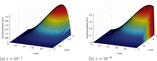
Figure 2. (a), (b) and (c) effect of the $\epsilon ,\delta$ and η on the behaviour of the solution with layer formation when $N=64=M$, respectively.

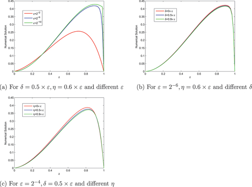
Figure 3. Example 4.1 Log-Log scale plot of the maximum absolute error for different values of ɛ.

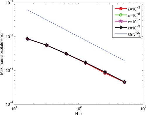
Table 1. $E_{\epsilon ,\delta ,\eta }^{N,\mathrm{\Delta }t},r_{\epsilon ,\delta ,\eta }^{N,\mathrm{\Delta }t},E^{N,\mathrm{\Delta }t}$and $r^{N,\mathrm{\Delta }t}$ for example 4.1 using the proposed method and results in (Sahu & Mohapatra, 2021) with $\delta =0.1\times \epsilon ,\eta =0.1\times \epsilon ,\xi =0.5\times \epsilon$

ɛ	N=16	32	64	128	256	512
$\downarrow$	M=8	16	32	64	128	256
Present Method
10^−3	8.6808$\times {10}^{-3}$	5.5873$\times {10}^{-3}$	3.1202$\times {10}^{-3}$	1.6719$\times {10}^{-3}$	8.3589$\times {10}^{-4}$	4.5042$\times {10}^{-4}$
	6.3568 $\times {10}^{-1}$	8.4051 $\times {10}^{-1}$	9.0015 $\times {10}^{-1}$	1.0001	8.9204 $\times {10}^{-1}$
10^−5	8.6852 $\times {10}^{-3}$	5.5901 $\times {10}^{-3}$	3.1225 $\times {10}^{-3}$	1.7041 $\times {10}^{-3}$	8.9350 $\times {10}^{-4}$	4.5725 $\times {10}^{-4}$
	6.3568 $\times {10}^{-1}$	8.4017 $\times {10}^{-1}$	8.7369 $\times {10}^{-1}$	9.3147 $\times {10}^{-1}$	9.6648 $\times {10}^{-1}$
10^−7	8.6852 $\times {10}^{-3}$	5.5901 $\times {10}^{-3}$	3.1225 $\times {10}^{-3}$	1.7041 $\times {10}^{-3}$	8.9350 $\times {10}^{-4}$	4.5725 $\times {10}^{-4}$
	6.3568 $\times {10}^{-1}$	8.4017 $\times {10}^{-1}$	8.7369 $\times {10}^{-1}$	9.3147 $\times {10}^{-1}$	9.6648 $\times {10}^{-1}$
10^−9	8.6852 $\times {10}^{-3}$	5.5901 $\times {10}^{-3}$	3.1225 $\times {10}^{-3}$	1.7041 $\times {10}^{-3}$	8.9350 $\times {10}^{-4}$	4.5725 $\times {10}^{-4}$
	6.3568 $\times {10}^{-1}$	8.4017$\times {10}^{-1}$	8.7369$\times {10}^{-1}$	9.3147$\times {10}^{-1}$	9.6648$\times {10}^{-1}$
$E^{N,\mathrm{\Delta }t}$	8.6852$\times {10}^{-3}$	5.5901$\times {10}^{-3}$	3.1225$\times {10}^{-3}$	1.7041$\times {10}^{-3}$	8.9350$\times {10}^{-4}$	4.5725$\times {10}^{-4}$
$r^{N,\mathrm{\Delta }t}$	6.3568$\times {10}^{-1}$	8.4017$\times {10}^{-1}$	8.7369$\times {10}^{-1}$	9.3147$\times {10}^{-1}$	9.6648$\times {10}^{-1}$
Results in (Sahu & Mohapatra, 2021)
10^−3	4.1480$\times {10}^{-2}$	2.8933$\times {10}^{-2}$	2.0069$\times {10}^{-2}$	1.3166$\times {10}^{-2}$	8.1760$\times {10}^{-3}$	4.8525$\times {10}^{-4}$
	0.5196	0.5277	0.6081	0.6873	0.7526
10^−5	4.1687$\times {10}^{-2}$	2.9042$\times {10}^{-2}$	2.0150$\times {10}^{-2}$	1.3216$\times {10}^{-2}$	8.2042$\times {10}^{-3}$	4.8694$\times {10}^{-3}$
	0.5214	0.5273	0.6084	0.6878	0.7526
10^−7	4.1689$\times {10}^{-2}$	2.9044$\times {10}^{-2}$	2.0151$\times {10}^{-2}$	1.3216$\times {10}^{-2}$	8.2045$\times {10}^{-3}$	4.8695$\times {10}^{-3}$
	0.5214	0.5273	0.6085	0.6878	0.7526
10^−9	4.1689$\times {10}^{-2}$	2.9044$\times {10}^{-2}$	2.0151$\times {10}^{-2}$	1.3216$\times {10}^{-2}$	8.2045$\times {10}^{-3}$	4.8695$\times {10}^{-3}$
	0.5214	0.5273	0.6085	0.6878	0.7526
$E^{N,\mathrm{\Delta }t}$	4.1689$\times {10}^{-2}$	2.9044$\times {10}^{-2}$	2.0151$\times {10}^{-2}$	1.3216$\times {10}^{-2}$	8.2045$\times {10}^{-3}$	4.8695$\times {10}^{-3}$
$r^{N,\mathrm{\Delta }t}$	0.5214	0.5273	0.6085	0.6878	0.7526

Table 2. $E_{\epsilon ,\delta ,\eta }^{N,\mathrm{\Delta }t},r_{\epsilon ,\delta ,\eta }^{N,\mathrm{\Delta }t},E^{N,\mathrm{\Delta }t}$and $r^{N,\mathrm{\Delta }t}$ for example 4.1 using the proposed method with $\epsilon ={10}^{-2},\xi =0.5\times \epsilon$

	N= 16	N=32	64	128	256	512
$\downarrow$	M=8	16	32	64	128	256
$\delta \downarrow$	$\eta =0.5\times \epsilon$
$0.1\times \epsilon$	8.0867$\times {10}^{-3}$	4.4416$\times {10}^{-3}$	2.6765$\times {10}^{-3}$	1.5293$\times {10}^{-3}$	8.2452$\times {10}^{-4}$	4.2998$\times {10}^{-4}$
	8.6447$\times {10}^{-1}$	7.3073$\times {10}^{-1}$	8.0748$\times {10}^{-1}$	8.9125$\times {10}^{-1}$	9.3928$\times {10}^{-1}$
$0.2\times \epsilon$	8.0782$\times {10}^{-3}$	4.4338$\times {10}^{-3}$	2.6713$\times {10}^{-3}$	1.5268$\times {10}^{-3}$	8.2302$\times {10}^{-4}$	4.2927$\times {10}^{-4}$
	8.6549$\times {10}^{-1}$	7.3100$\times {10}^{-1}$	8.0703$\times {10}^{-1}$	8.9151$\times {10}^{-1}$	9.3904$\times {10}^{-1}$
$0.3\times \epsilon$	8.0699$\times {10}^{-3}$	4.4259$\times {10}^{-3}$	2.6661$\times {10}^{-3}$	1.5242$\times {10}^{-3}$	8.2151$\times {10}^{-4}$	4.2856$\times {10}^{-4}$
	8.6658$\times {10}^{-1}$	7.3124$\times {10}^{-1}$	8.0668$\times {10}^{-1}$	8.9170$\times {10}^{-1}$	9.3878$\times {10}^{-1}$
$0.4\times \epsilon$	8.0624$\times {10}^{-3}$	4.4180$\times {10}^{-3}$	2.6609$\times {10}^{-3}$	1.5216$\times {10}^{-3}$	8.1998$\times {10}^{-4}$	4.2784$\times {10}^{-4}$
	8.6782$\times {10}^{-1}$	7.3148$\times {10}^{-1}$	8.0633$\times {10}^{-1}$	8.9193$\times {10}^{-1}$	9.3852$\times {10}^{-1}$
$0.5\times \epsilon$	8.0548$\times {10}^{-3}$	4.4101$\times {10}^{-3}$	2.6557$\times {10}^{-3}$	1.5189$\times {10}^{-3}$	8.1863$\times {10}^{-4}$	4.2711$\times {10}^{-4}$
	8.6904$\times {10}^{-1}$	7.3172$\times {10}^{-1}$	8.0607$\times {10}^{-1}$	8.9174$\times {10}^{-1}$	9.3860$\times {10}^{-1}$
$E^{N,\mathrm{\Delta }t}$	8.0867$\times {10}^{-3}$	4.4416$\times {10}^{-3}$	2.6765$\times {10}^{-3}$	1.5293$\times {10}^{-3}$	8.2452$\times {10}^{-4}$	4.2998$\times {10}^{-4}$
$r^{N,\mathrm{\Delta }t}$	8.6447$\times {10}^{-1}$	7.3073$\times {10}^{-1}$	8.0748$\times {10}^{-1}$	8.9125$\times {10}^{-1}$	9.3928$\times {10}^{-1}$
$\eta \downarrow$	$\delta =0.5\times \epsilon$
$0.1\times \epsilon$	8.0787$\times {10}^{-3}$	4.4351$\times {10}^{-3}$	2.6733$\times {10}^{-3}$	1.5271$\times {10}^{-3}$	8.2315$\times {10}^{-4}$	4.2930$\times {10}^{-4}$
	8.6516$\times {10}^{-1}$	7.3034$\times {10}^{-1}$	8.0783$\times {10}^{-1}$	8.9157$\times {10}^{-1}$	9.3917$\times {10}^{-1}$
$0.2\times \epsilon$	8.0727$\times {10}^{-3}$	4.4289$\times {10}^{-3}$	2.6689$\times {10}^{-3}$	1.5251$\times {10}^{-3}$	8.2195$\times {10}^{-4}$	4.2873$\times {10}^{-4}$
	8.6610$\times {10}^{-1}$	7.3070$\times {10}^{-1}$	8.0734$\times {10}^{-1}$	8.9178$\times {10}^{-1}$	9.3898$\times {10}^{-1}$
$0.3\times \epsilon$	8.0667$\times {10}^{-3}$	4.4226$\times {10}^{-3}$	2.6646$\times {10}^{-3}$	1.5230$\times {10}^{-3}$	8.2077$\times {10}^{-4}$	4.2818$\times {10}^{-4}$
	8.6708$\times {10}^{-1}$	7.3098$\times {10}^{-1}$	8.0700$\times {10}^{-1}$	8.9187$\times {10}^{-1}$	9.3876$\times {10}^{-1}$
$0.4\times \epsilon$	8.0607$\times {10}^{-3}$	4.4163$\times {10}^{-3}$	2.6601$\times {10}^{-3}$	1.5210$\times {10}^{-3}$	8.1962$\times {10}^{-4}$	4.2764$\times {10}^{-4}$
	8.6807$\times {10}^{-1}$	7.3136$\times {10}^{-1}$	8.0646$\times {10}^{-1}$	8.9199$\times {10}^{-1}$	9.3856$\times {10}^{-1}$
$0.5\times \epsilon$	8.0548$\times {10}^{-3}$	4.4101$\times {10}^{-3}$	2.6557$\times {10}^{-3}$	1.5189$\times {10}^{-3}$	8.1863$\times {10}^{-4}$	4.2711$\times {10}^{-4}$
	8.6904$\times {10}^{-1}$	7.3172$\times {10}^{-1}$	8.0607$\times {10}^{-1}$	8.9174$\times {10}^{-1}$	9.3860$\times {10}^{-1}$
$E^{N,\mathrm{\Delta }t}$	8.0787$\times {10}^{-3}$	4.4351$\times {10}^{-3}$	2.6733$\times {10}^{-3}$	1.5271$\times {10}^{-3}$	8.2315$\times {10}^{-4}$	4.2930$\times {10}^{-4}$
$r^{N,\mathrm{\Delta }t}$	8.6516$\times {10}^{-1}$	7.3034$\times {10}^{-1}$	8.0783$\times {10}^{-1}$	8.9157$\times {10}^{-1}$	9.3917$\times {10}^{-1}$

Figure 1. Example 4.1 Log–Log scale plot of the maximum absolute error for different values of ɛ.

5. Conclusion

A parameter uniform numerical scheme for singularly perturbed parabolic differential-difference equation with delay in time is presented. The developed scheme constitutes the implicit Euler in the time direction and the exponential cubic spline method in the space direction. The stability and parameter uniform convergence of the proposed scheme are investigated. The scheme is shown to be uniformly convergent with a linear order of convergence. A test example is presented to illustrate the efficiency of the proposed scheme. It is observed that the proposed computational technique gives more accurate numerical results than the method in (Sahu & Mohapatra, 2021).

Acknowledgements

The authors thankfully acknowledge the prolific comments from the anonymous referees.

Disclosure statement

No potential conflict of interest was reported by the author(s).

Funding

This research did not receive any funding.

Data availability statement

No data were used to support the study.

Additional information

Funding

This work was supported by the No fund.

Notes on contributors

Genanew Gofe Gonfa

Genanew Gofe Gonfa received his Ph.D. in Mathematics from Andhra University, India. He is presently working at Salale University as an associate professor of Mathematics and President, Salale University, Ethiopia. His research interests span on the areas of numerical solutions of differential equations, systems of equations, and singularly perturbed ordinary and partial differential equations. He published more than 13 research articles in national and international reputable journals. In addition, he made numerous contributions in serving as a reviewer, assistant editor, and editor for various national and international reputable journals. So far, he has supervised 40 M.Sc. graduates to completion and currently supervising 8 M.Sc. students.

Imiru Takele Daba

Imiru Takele Daba received his Ph.D. in Mathematics from Wollega University in 2021. His research interests span the areas of numerical solutions of partial differential equations, focusing on singularly perturbed problems. He has published more than 13 research articles in reputable journals. He also made numerous contributions while serving as a reviewer. So far, he has supervised 19 M.Sc. students to completion and currently supervising 8 M.Sc. students.

References

- Chandru, M., Prabha, T., Das, P., & Shanthi, V. (2019). A numerical method for solving boundary and interior layers dominated parabolic problems with discontinuous convection coefficient and source terms. Differential Equations and Dynamical Systems, 27, 91–112. https://doi.org/10.1007/s12591-017-0385-3
- Daba, I. T, & Duressa, G. F. (2021). A hybrid numerical scheme for singularly perturbed parabolic differential-difference equations arising in the modeling of neuronal variability. Computational and Mathematical Methods, 3(5), e1178. https://doi.org/10.1002/cmm4.1178
- Daba, I. T., & Duressa, G. F. (2021a). Extended cubic B-spline collocation method for singularly perturbed parabolic differential-difference equation arising in computational neuroscience. International Journal for Numerical Methods in Biomedical Engineering, 37(2). https://doi.org/10.1002/cnm.3418
- Daba, I. T., & Duressa, G. F. (2021b). Hybrid algorithm for singularly perturbed delay parabolic partial differential equations. Applications and Applied Mathematics: An International Journal (AAM), 16(1), 21.
- Daba, I. T., & Duressa, G. F. (2021c). Uniformly convergent numerical scheme for a singularly perturbed differential-difference equations arising in computational neuroscience. Journal of Applied Mathematics & Informatics, 39(5–6), 655–676.
- Daba, I. T., & Duressa, G. F. (2022a). Collocation method using artificial viscosity for time dependent singularly perturbed differential–difference equations. Mathematics and Computers in Simulation, 192, 201–220. https://doi.org/10.1016/j.matcom.2021.09.005
- Daba, I. T., & Duressa, G. F. (2022b). A novel algorithm for singularly perturbed parabolic differential-difference equations. Research in Mathematics, 9(1), 2133211. https://doi.org/10.1080/27684830.2022.2133211
- Daba, I. T., & Duressa, G. F. (2022c). A robust computational method for singularly perturbed delay parabolic convection-diffusion equations arising in the modeling of neuronal variability. Computational Methods for Differential Equations, 10(2), 475–488.
- Das, P., & Natesan, S. (2012). Higher-order parameter uniform convergent schemes for Robin type reaction-diffusion problems using adaptively generated grid. International Journal of Computational Methods, 9(4), 1250052. https://doi.org/10.1142/S0219876212500521
- Das, P., & Natesan, S. (2013). A uniformly convergent hybrid scheme for singularly perturbed system of reaction-diffusion Robin type boundary-value problems. Journal of Applied Mathematics and Computing, 41, 447–471. https://doi.org/10.1007/s12190-012-0611-7
- Das, P., Rana, S., & Ramos, H. (2019). Homotopy perturbation method for solving Caputo-type fractional-order Volterra-fredholm integro-differential equations. Computational and Mathematical Methods, 1(5), e1047. https://doi.org/10.1002/cmm4.1047
- Das, P., Rana, S., & Ramos, H. (2020). A perturbation-based approach for solving fractional-order Volterra-fredholm integro differential equations and its convergence analysis. International Journal of Computer Mathematics, 97(10), 1994–2014. https://doi.org/10.1080/00207160.2019.1673892
- Das, P., Rana, S., & Ramos, H. (2022). On the approximate solutions of a class of fractional order nonlinear Volterra integro-differential initial value problems and boundary value problems of first kind and their convergence analysis. Journal of Computational and Applied Mathematics, 404, 113116. https://doi.org/10.1016/j.cam.2020.113116
- Das, P., Rana, S., & Vigo-Aguiar, J. (2020). Higher order accurate approximations on equidistributed meshes for boundary layer originated mixed type reaction diffusion systems with multiple scale nature. Applied Numerical Mathematics, 148, 79–97. https://doi.org/10.1016/j.apnum.2019.08.028
- Das, P., & Vigo-Aguiar, J. (2019). Parameter uniform optimal order numerical approximation of a class of singularly perturbed system of reaction diffusion problems involving a small perturbation parameter. Journal of Computational and Applied Mathematics, 354, 533–544. https://doi.org/10.1016/j.cam.2017.11.026
- Das, P. (2015). Comparison of a priori and a posteriori meshes for singularly perturbed nonlinear parameterized problems. Journal of Computational and Applied Mathematics, 290, 16–25. https://doi.org/10.1016/j.cam.2015.04.034
- Das, P. (2018). A higher order difference method for singularly perturbed parabolic partial differential equations. Journal of Difference Equations and Applications, 24(3), 452–477. https://doi.org/10.1080/10236198.2017.1420792
- Das, P. (2019). An a posteriori based convergence analysis for a nonlinear singularly perturbed system of delay differential equations on an adaptive mesh. Numerical Algorithms, 81(2), 465–487. https://doi.org/10.1007/s11075-018-0557-4
- Doolan, E. P., Miller, J. J. H., & Schilders, W. H. A. (1980). Uniform numerical methods for problems with initial and boundary layers. Boole Press.
- Govindarao, L., & Mohapatra, J. (2020). Numerical analysis and simulation of delay parabolic partial differential equation involving a small parameter. Engineering Computations, 37(1), 289–312. https://doi.org/10.1108/EC-03-2019-0115
- Govindarao, L., Sahu, S. R., & Mohapatra, J. (2019). Uniformly convergent numerical method for singularly perturbed time delay parabolic problem with two small parameters. Iranian Journal of Science & Technology, Transactions A: Science, 43(5), 2373–2383. https://doi.org/10.1007/s40995-019-00697-2
- Govindarao, S. R., Mohapatra, J., & Sahu, L. (2019). Uniformly convergent numerical method for singularly perturbed two parameter time delay parabolic problem. International Journal of Applied and Computational Mathematics, 5(3), 1–9. https://doi.org/10.1007/s40819-019-0672-5
- Gupta, V., Kadalbajoo, M. K., & Dubey, R. K. (2019). A parameter-uniform higher order finite difference scheme for singularly perturbed time-dependent parabolic problem with two small parameters. International Journal of Computer Mathematics, 96(3), 474–499. https://doi.org/10.1080/00207160.2018.1432856
- Kumar, D. (2018). An implicit scheme for singularly perturbed parabolic problem with retarded terms arising in computational neuroscience. Numerical Methods for Partial Differential Equations, 34(6), 1933–1952. https://doi.org/10.1002/num.22269
- Musila, M., & Lánsk’y, P. (1991). Generalized stein’s model for anatomically complex neurons. BioSystems, 25(3), 179–191. https://doi.org/10.1016/0303-2647(91)90004-5
- Nageshwar Rao, R., & Chakravarthy, P. (2019). Fitted numerical methods for singularly perturbed one-dimensional parabolic partial differential equations with small shifts arising in the modelling of neuronal variability. Differential Equations and Dynamical Systems, 27(1–3), 1–18. https://doi.org/10.1007/s12591-017-0363-9
- Negero, N. T., & Duressa, G. F. (2022). An efficient numerical approach for singularly perturbed parabolic convection-diffusion problems with large time-lag. Journal of Mathematical Modeling, 10(2), 173–190.
- Nichols, N. (1989). On the numerical integration of a class of singular perturbation problems. Journal of Optimization Theory and Applications, 60(3), 2050034. https://doi.org/10.1007/BF00940347
- O’Malley, J. R. E. (1974). Introduction to singular perturbations. Technical report. New York Univ Ny Courant Inst of Mathematical Sciences. https://apps.dtic.mil/sti/citations/AD0787833.
- Ramesh, V. P., & Priyanga, B. (2019). Higher order uniformly convergent numerical algorithm for time-dependent singularly perturbed differential-difference equations. Differential Equations and Dynamical Systems, 29(1), 239–263. https://doi.org/10.1007/s12591-019-00452-4
- Reddy, N. R., & Mohapatra, J. (2023). A robust numerical scheme for singularly perturbed delay parabolic initial-boundary value problems involving mixed space shifts. Computational Methods for Differential Equations, 11(1), 42–51.
- Roos, H.-G., Martin, S., & Tobiska, L. (2008 24). Robust numerical methods for singularly perturbed differential equations: Convection-diffusion-reaction and flow problems. Springer Science & Business Media.
- Sahu, S. R., & Mohapatra, J. (2021). Numerical study of time delay singularly perturbed parabolic differential equations involving both small positive and negative space shift. Journal of Applied Analysis, 28(1), 121–134. https://doi.org/10.1515/jaa-2021-2064
- Saini, S., Das, P., & Kumar, S. (2023). Computational cost reduction for coupled system of multiple scale reaction diffusion problems with mixed type boundary conditions having boundary layers. Revista de la Real Academia de Ciencias Exactas Físicas y Naturales Serie A Matemáticas, 117(2), 66. https://doi.org/10.1007/s13398-023-01397-8
- Shakti, D., Mohapatra, J., Das, P., & Vigo-Aguiar, J. (2022). A moving mesh refinement based optimal accurate uniformly convergent computational method for a parabolic system of boundary layer originated reaction?diffusion problems with arbitrary small diffusion terms. Journal of Computational and Applied Mathematics, 404, 113167. https://doi.org/10.1016/j.cam.2020.113167
- Shiromani, R., Shanthi, V., & Das, P. (2023). A higher order hybrid-numerical approximation for a class of singularly perturbed two-dimensional convection-diffusion elliptic problem with non-smooth convection and source terms. Computers & Mathematics with Applications, 142, 9–30. https://doi.org/10.1016/j.camwa.2023.04.004
- Shishkin, G. I., & Shishkina, L. P. (2008). Difference methods for singular perturbation problems. CRC Press.
- Srivastava, H. M., Nain, A. K., Vats, R. K., & Das, P. (2023). A theoretical study of the fractional-order p-Laplacian nonlinear hadamard type turbulent flow models having the ulam-Hyers stability. Revista de la Real Academia de Ciencias Exactas Físicas y Naturales Serie A Matemáticas, 117(4), 160. https://doi.org/10.1007/s13398-023-01488-6
- Sumit, K., Kuldeep, S., Kumar, M., & Kumar, M. (2020). A robust numerical method for a two-parameter singularly perturbed time delay parabolic problem. Computational & Applied Mathematics, 39(3). https://doi.org/10.1007/s40314-020-01236-1
- Tian, H. (2002). The exponential asymptotic stability of singularly perturbed delay differential equations with a bounded lag. Journal of Mathematical Analysis and Applications, 270(1), 143–149. https://doi.org/10.1016/S0022-247X(02)00056-2
- Wang, P. K. C. (1963). Asymptotic stability of a time-delayed diffusion system. Journal of Applied Mechanics, 30(4), 500–504. https://doi.org/10.1115/1.3636609
- Zahra, W. K., & Ashraf, M. E. M. (2013). Numerical solution of two-parameter singularly perturbed boundary value problems via exponential spline. Journal of King Saud University-Science, 25(3), 201–208. https://doi.org/10.1016/j.jksus.2013.01.003