
 ?Mathematical formulae have been encoded as MathML and are displayed in this HTML version using MathJax in order to improve their display. Uncheck the box to turn MathJax off. This feature requires Javascript. Click on a formula to zoom.
ABSTRACT
In this paper, we propose a uniformly convergent numerical scheme for a class of time-fractional singularly perturbed delay partial differential equations exhibiting a right regular boundary layer. The time-fractional derivative is considered in the Caputo sense with order . The domain is discretized with a uniform mesh in both time and space directions. The numerical scheme comprises the discretization technique given by the Crank–Nicolson method in the temporal direction and the non-standard finite difference method in the spatial direction. To show the parameter uniform convergence of the proposed method, the boundedness of truncation error and stability analysis are performed. It is shown that the proposed scheme is second-order convergent in the temporal direction and first-order convergent in the spatial direction. Numerical examples are presented, and their numerical simulations confirm the theoretical findings.
1. Introduction
Delay partial differential equations (DPDEs) give a more realistic model of physical problems by considering both the past history and the present state of the system (Ansari et al., Citation2007). Often, the delay accounts for the time it takes for the process to occur. For example, gestation times, incubation periods, and transport delays. DPDEs have many applications in science and engineering (Kumar & Kumari, Citation2019). When the highest spatial derivative of the DPDE is multiplied by a small parameter , it is said to be singularly perturbed delay partial differential equation (SPDPDE), and ϵ is said to be a perturbation parameter. As the perturbation parameter ϵ → 0, the solution exhibits a boundary or an interior layer. Due to the existence of a boundary or an interior layer on the solution of SPDPDE, when we apply standard numerical methods like the finite difference method, the finite element method, and the finite volume method to a uniform mesh, large oscillations occur in the computed solution, leading to numerical instability and inaccurate solutions (Gowrisankar & Natesan, Citation2017). To overcome this difficulty, ϵ - uniformly convergent numerical methods, that is, numerical methods whose convergence property, accuracy, and computational cost do not depend on the perturbation parameter and only depend on the number of mesh points, must be developed (Miller et al., Citation1996).
In general, there are two kinds of ϵ - uniform numerical methods for solving singularly perturbed problems in the context of finite difference methods. Namely, fitted operator methods (FOMs) and fitted mesh methods (FMMs). In FOMs, exponential fitting factor or positive denominator function can be used to control the rapid change of the solution in the boundary or interior layer region(s). When we use exponential fitting factor and denominator function on a term containing perturbation parameter, the methods are said to be the exponentially fitted operator method (EFOM) and the non-standard finite difference method (NSFDM), respectively. Whereas, FMMs employ non-uniform meshes that will be fine in the boundary layer region and coarse outside the boundary layer region(s).
In the past few decades, fractional calculus has gained more attention because of its wide applications in science and engineering (Sun et al., Citation2018). It is a generalization of classical calculus to arbitrary-order derivatives and integrals and can be used in the oil industry, neural networks, mass transport in fluids, control theory, signal processing, viscoelasticity, rheology, finance, dispersion of pollutants in the atmosphere, and so on (Kilbas et al., Citation2006). Due to the non-local properties of fractional derivative and integral operators, they are used to model memory effects and hereditary properties of physical problems more accurately than integer-order derivative and integral operators, which are neglected in the integer-order integral and derivative operators. Fractional partial differential equations (FPDEs) that are described by non-integer-order derivatives model many complex systems such as anomalous diffusion, viscoelastic materials, etc. (Dai et al., Citation2015). Due to the widespread application of FPDEs in engineering and science, this area has been receiving significant attention, and as a result, numerous analytical (Ata & Kıymaz, Citation2023; Atangana, Citation2014; Chen et al., Citation2007), semi-analytical (Daraghmeh et al., Citation2020; Odibat & Momani, Citation2006), and numerical methods (Karatay & Bayramoglu, Citation2012; Kumar et al., Citation2022; Lin & Xu, Citation2007) were introduced to solve FPDEs.
In this paper, we consider the following time-fractional singularly perturbed delay partial differential equation (TF-SPDPDE):
with the interval and boundary conditions:
where denotes the perturbation parameter, η > 0 denotes the delay parameter
. Here, the domain be
and
is its boundary, where
and
are the left and right sides of
corresponding to x = 0 and 1, respectively, and
. Also,
is the Caputo time-fractional derivative of order
, usually denoted by
and defined by
where Γ represents the gamma function defined as for with
If , the problem given in EquationEquation (1)
(1)
(1) is a TF-SPDPDE, which is the generalization of classical SPDPDE. This type of problem is widely used in oil reservoir simulations, transport of mass and energy, dispersion of chemicals in reactors, etc. (Choudhary et al. (Citation2022).
Suppose that and
are bounded smooth functions in the rectangular domain
. In addition, let us assume that the initial boundary functions given are sufficiently smooth and satisfy the following compatibility condition at the corner points of
(i.e. at
and
). This means
Under these sufficiently smooth assumptions and compatibility conditions imposed on the initial and boundary data, the interval boundary value problem (1)-(2) admits a unique solution that exhibits a regular boundary layer of width
at
, as the perturbation parameter becomes very small
. Due to the non-locality of the fractional derivative operator and the involvement of delay and perturbation parameters, it is not simple to solve this problem effectively and more accurately. Hence, designing the ϵ - uniform numerical methods for such type of problems is an important task and is the objective of the present work.
There have been several investigations into the cases of numerical treatment of integer-order singularly perturbed delay partial differential equations. (e.g. see (Ansari et al., Citation2007; Bashier & Patidar, Citation2011; Duressa et al., Citation2023; Govindarao & Mohapatra, Citation2018; Kumar & Kumari, Citation2020; Negero & Duressa, Citation2022; Tirunehi et al., Citation2023) and the references therein). Moreover, FPDEs that are not singularly perturbed have been widely studied up to now. For example, Rihan (Citation2010) presented fully implicit - methods to solve linear and non-linear time-fractional delay partial differential equations. Qiu et al. (Citation2019) developed a numerical method comprising the L1 scheme and central finite difference approximation formula to solve one-dimensional time-fractional Burgers equation. The method was shown unconditional stable and convergent of order 2−α, α ∈ (0, 1) in the temporal direction and of order two in spatial direction. Choudhary et al. (Citation2022) proposed a second-order convergent numerical scheme for a class of time-fractional partial differential equations with delay in time. The authors used a numerical method comprising the Crank–Nicolson method for time discretization and Spline method with a tension factor for spatial discretization on a uniform mesh. However, the problems considered in the works above are not singularly perturbed. Relatively, if the problems are not singularly perturbed (in the absence of the perturbation parameter), then we may not face numerical difficulties to find their numerical solution
However, few studies are conducted on the numerical treatment of time-fractional singularly perturbed delay partial differential equations. For instance, Liu et al. (Citation2021) designed a stable numerical scheme to solve a one- and two-dimensional time-fractional singularly perturbed partial differential equation with variable coefficients. They employed the Tailored finite point method to approximate the space derivative and the Grunwald-Letnikov and L1 scheme to approximate the time-fractional derivative. The scholars (Kumar & Vigo-Aguiar, Citation2021) developed a uniformly convergent numerical scheme to obtain an approximate solution of singularly perturbed time-fractional partial differential equations with delay in time. They used the L1 scheme on a uniform mesh to approximate the time-fractional derivative and stable finite difference method with piecewise uniform meshes (which are adequate for FMMs) for approximating the spacial derivatives. Motivated by the study of (Kumar, Kamalesh and Vigo-Aguiar, J, 2021), the purpose of this paper is to design - uniformly convergent numerical method to solve time-fractional singularly perturbed partial differential equations with a large time delay given in Equationequations (1)
(1)
(1) -(Equation2
(2)
(2) ). We apply the Crank–Nicolson method and the NSFDM to approximate the time-fractional and space derivatives, respectively. Since NSFDM is one of a class of FOM, it has the advantage over FMM that it does not require any prior information about the location and width of the boundary layer(s).
1.1. Properties of the continuous problem
In this section, we present some properties of the continuous problem given in EquationEquation (1)(1)
(1) -EquationEquation (2)
(2)
(2) , which are important to analyze the semi-discrete and the full-discrete schemes of the continuous problem that we will discuss in the next sections.
Lemma 1.1.
The Continuous Maximum principle Let satisfying
and
. Then
.
Proof.
Let us assume that there exists such that
and . From the given hypothesis, we have
and
. As
attains minimum at
we have
and
and since
, we obtain the following:
which contradicts the assumption in
. Hence,
. Therefore, we conclude that
.
Lemma 1.2.
The solution of the continuous problem (1)-(2) satisfy the following estimate
Proof.
Using the compatibility conditions at the corner points (i.e. ) and applying Lemma 1.1 on the barrier functions defined by
gives the required estimate. To show this, we have
On the boundary
Additionally, for
since C can be chosen sufficiently large.
Therefore, using the maximum principle (Lemma 1.1), we get
This implies that
Lemma 1.3.
The solution of the problem (1)-(2) satisfy the following bound:
Proof.
For all , we have
Using Lemma 1.2 and the fact that is bounded, we get the required result.
Lemma 1.4.
(Stability Estimate of the continuous problem) Let be the solution of problem (1)-(2). Then, we have
Proof.
Define the barrier functions
Thus we have
Also, for
Moreover, for
Therefore, by using Lemma 1.1, we get the required result.
2. Numerical scheme
In this section, we present parameter uniformly convergent numerical scheme to approximate the problem given in (1)-(2) by discretizing both the time and space variables with a uniform mesh. To design the scheme, we first discretize the temporal variable using the Crank–Nicolson method. Next, the semi-discretized problem is numerically approximated by using the non-standard finite difference method with a simple upwind finite difference method in the spatial direction.
2.1. Time discretization
The use of Taylor’s series expansion for the term containing the large delay η in EquationEquation (1)(1)
(1) is invalid because of Taylor’s series approximation gives better results when η is small. To address this challenge, first we discretize the time domain
into the N subinterval with a uniform step size
and by choosing K in such a way that
for some positive integer
Thus, we have
Now we semi-discretize the problem (1) on as follows:
By Taylor series expansion with center at the point we have
and
Subtracting EquationEquation (5)(5)
(5) from EquationEquation (4)
(4)
(4) , we get the following:
Next, we approximate the Caputo fractional derivative in the following approach.
Using a second-order central finite difference approximation for the first-order derivative given in EquationEquation (6)(6)
(6) , we obtain the following equation.
Rearranging the above row of EquationEquation (7)(7)
(7) , we get an equivalent equation of the form:
Let
Substituting EquationEquations (9)(9)
(9) , (Equation10
(10)
(10) ) and (Equation11
(11)
(11) ) into EquationEquation (8)
(8)
(8) , we get
EquationEquation (12)(12)
(12) can be equivalently written as
Hence, the Crank–Nicolson approximation of the Caputo fractional derivative at is given by
Thus, from EquationEquation (15)(15)
(15) , we observed a second-order approximation to
This means that the Crank–Nicolson scheme is a second-order convergence for the time-fractional derivative.
Substituting EquationEquation (15)(15)
(15) by neglecting the truncation error into EquationEquation (3)
(3)
(3) , we have the following approximation formula:
where represents the approximate solution of the exact solution
at
time level. Now, introducing the notation
into the above Equation and rearranging, we get the following equivalent form:
where
Rearranging EquationEquation (17)(17)
(17) , we get the following equivalent form.
Using discrete operator, EquationEquation (18)(18)
(18) can be written as
where
with the interval boundary conditions:
The operator is defined as
satisfies the next semi-discrete maximum principle.
Lemma 2.1.
(The Semi-discrete maximum principle) Let be a smooth function on
. If
and
then
Proof.
To proof is done by contradiction. Let such that
and assume that . From the hypotheses, we have
and
, hence
which is a contradiction to our assumption of in
. This shows that our assumption is wrong and then
Therefore, we conclude that
.
Theorem 2.2.
Under the smoothness and compatibility conditions, the semi-discretized solution and its derivatives satisfy the following bounds:
Proof.
The proof is found in (Kellogg et al., Citation1978).
2.2. Spatial discretization
Now, we consider the spatial discretization of EquationEquation (32)(32)
(32) by the non-standard finite difference method on a uniform mesh. Let M be a positive integer and divide the domain
into M equal sub-intervals with step size
:
To discretize the space derivatives using the method of non-standard finite difference scheme on a uniform mesh, we will follow the procedures used in (Mickens Citation2005). Using these principles, the denominator function denoted by is given by (Mbroh et al., Citation2019)
Let represent the approximation of
Using this denominator function and the simple upwind finite difference approximation for the first derivative of EquationEquation (32)
(32)
(32) , we obtain the following fully-discrete problem.
with the interval boundary conditions:
After making some rearrangement, we have the following equation.
Equivalently, we write EquationEquation (32)(32)
(32) in linear system form as follows:
where
Since we let in the domain
, again let us suppose that
Lemma 2.3.
(The Fully-discrete Maximum Principle). Assume that the discrete function satisfying
and
. Then
for all
.
Proof.
Let be the indexes such that
Then by the given hypothesis, we have . It follows that
Hence,
This shows that our assumption is wrong and Therefore, we have
.
An immediate consequence of Lemma 2.3 is the uniform stability estimate given below.
Lemma 2.4.
The solution of the fully-discretized problem in EquationEquation (32)
(32)
(32) satisfy the following bound.
Proof.
Let us denote
and define the barrier functions
At the boundary points
On the discretized domain we have
By Lemma 2.3, we obtain , for all
. This implies that
In the next section, we estimate the error associated with the spatial discretization.
3. Convergence analysis
By using the information presented above, we were able to demonstrate that the fully- discrete operator denoted by satisfies both the discrete maximum principle and the uniform stability estimate. Let
denotes the approximate solution in the fully-discretization of the exact solution
at
Next, let us denote and define the forward, backward and central finite difference approximations of the space derivatives, respectively, as
Then, the truncation error of the scheme (24)-(25) is given by
Here, we have To show this, let us define
Using EquationEquation (23)
(23)
(23) , we obtain the following relation:
Because of we have
Using this relation, we have the following:
So, the error estimate in the spatial discretization is bounded as
Using the boundedness of derivatives of solution given in Theorem 2.2 and EquationEquation (29)(29)
(29) , we obtain
Lemma 3.1.
For a fixed mesh and ϵ → 0, it holds
where for all
Proof.
The proof is found in (Turuna et al., Citation2020).
Using the result of Lemma 3.1 into EquationEquation (30)(30)
(30) , we obtain
Define the barrier functions
The values at boundaries are
Using maximum principle, we have
From this it follows that
Theorem 3.2.
(ϵ-uniform convergence) If be the exact solution of the continuous problem EquationEquation (1)
(1)
(1) -EquationEquation (2)
(2)
(2) and
be the numerical solution of the fully discretized scheme EquationEquation (32)
(32)
(32) -EquationEquation (32)
(32)
(32) , then the following error estimate holds
Proof.
From EquationEquation (14)(14)
(14) and EquationEquation (32)
(32)
(32) , we can obtain the above error bound. To show this,
4. Numerical examples
To show the effectiveness of the proposed scheme given in EquationEquation (26)(26)
(26) for the given problem (1), we consider the following two examples. Since the exact solution to these problems is not known, to determine the maximum pointwise error and rate of convergence, we use the double mesh principle (Doolan et al., Citation1980). To apply this technique, the space and time domains are divided into 2 M and 2 N equal sub-intervals respectively. Then, the maximum pointwise error and the convergence rate are obtained as follows. The maximum pointwise error is
where denotes the numerical solution obtained on a mesh containing M +1 points in the spatial direction and N +1 points in the temporal direction, and
is obtained by further dividing each sub-interval in space and time direction. In addition, the rate of convergence of the problems are obtained by the formula
Example 4.1.
Consider the following time-fractional singularly perturbed parabolic partial differential equation with delay η = 1:
with the interval and boundary conditions
Example 4.2.
Consider the following time-fractional singularly perturbed parabolic partial differential equation with delay η = 1:
with the interval and boundary conditions
For different values of and fixed β = 0.8, the maximum pointwise error and the corresponding rate of convergence for Example 4.1 and Example 4.2 are given in Tables and respectively. The last two rows in these tables represent the ϵ- uniform error estimate
and the ϵ- uniform convergence rate
Similarly, for different values of
and M with fixed
, the maximum pointwise error and the rate of convergence are given in Tables and respectively. From the Tables , one can clearly observe that the maximum pointwise error decreases monotonically as the mesh size M and N increases, which confirms that the proposed scheme is ϵ - uniformly convergent. To show the existence of boundary layer near x = 1 for small ϵ (ϵ → 0), the surface plots of solutions of Example 4.1 and Example 4.2 are given in Figures and respectively for different values of β. In addition, to show the effect of ϵ on the width of the boundary layer, the surface plots of solutions of Example 4.1 and Example 4.2 are given in Figures and respectively. Similarly, to show the effects of the fractional order β on the solution of Example 4.1 and Example 4.2, the surface plots are given in Figures and respectively. Figure shows the log-log plot of the maximum pointwise error for the solutions for Example 4.1 and Example 4.2. From this figure, one can observe the parameter uniform convergence of the proposed method. Moreover, the formulated scheme is shown to be first-order convergence globally.
Figure 1. Surface plots of the numerical solution of example 4.1 for different values of β with and N = 64.
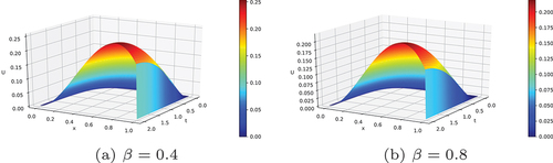
Figure 2. Surface plots of the numerical solution of example 4.1 for different values of ϵ with and N = 64.
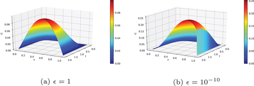
Figure 3. Surface plots of the numerical solution of example 4.2 for different values of β with and N = 64.
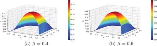
Figure 4. Surface plots of the numerical solution of example 4.2 for different values of ϵ with and N = 64.
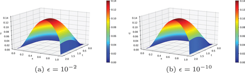
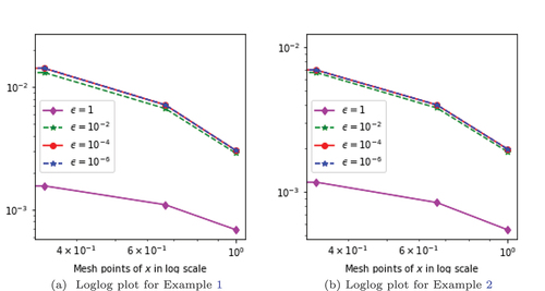
Table 1. Maximum pointwise error and rate of convergence
for example 4.1 using fractional order β = 0.8 with different values of
Table 2. Maximum pointwise error and rate of convergence
for example 4.1 using
with different values of β
Table 3. Maximum pointwise error and rate of convergence
for example 4.2 using fractional order β = 0.8 with different values of ϵ
Table 4. Maximum pointwise error and rate of convergence
for example 4.2 using
with different values of β
5. Conclusion
In this paper, a parameter uniformly convergent numerical scheme for a class of time-fractional singularly perturbed partial differential equations with a large time delay is considered. The proposed numerical scheme consists of the Crank–Nicolson method for discretizing the time-fractional derivative, which is given in Caputo sense and the non-standard finite difference method together with simple upwind scheme to discretize the spatial derivatives on a uniform mesh. The method is shown to be second-order accurate with respect to the time variable and first-order accurate with respect to the space variable. Moreover, the proposed method is uniformly convergent with respect to the perturbation parameter ϵ. To validate the theoretical predictions, numerical experimentation is performed and the numerical results support the theoretical findings.
It is very important to note that previously the method of Crank–Nicolson and NSFDM are developed for only integer order singularly perturbed delay partial differential equations. According to the best of our knowledge, this has not been done so far for the case of TF-SPDPDEs. Hence, this is the first work based on the fractional order singularly perturbed delay partial differential equations. In the future, we will extend this work for higher order numerical schemes to solve TF-SPDPDEs.
PUBLIC INTEREST STATEMENT
Nowadays, due to the non-locality of fractional differential operators, it is confirmed that many anomalous diffusion processes associated with complex systems in science and engineering are described more accurately by fractional partial differential equations than classical partial differential equations. If the small perturbation parameter multiplies the highest order derivative of the time-fractional partial differential equation and when it contains the delay parameter, then the problem is singularly perturbed time-fractional delay partial differential equation. The solution of such types of problems exhibit boundary layer phenomena. Due to the existence of boundary layer in the solution, if we use classical numerical methods, large oscillations occur in the computed solution, leading to numerical instability and inaccurate solution. To overcome this problem, we developed uniformly convergent numerical method with respect to the perturbation parameter.
sn-sample-bib.tex
Download Latex File (1.1 KB)Disclosure statement
No potential conflict of interest was reported by the author(s).
Supplementary material
Supplemental data for this article can be accessed online at https://doi.org/10.1080/27684830.2023.2293373.
Additional information
Notes on contributors
Habtamu Getachew Kumie
Awoke Andargie Tirunehi is an Associate Professor of Mathematics and member of Department of Mathematics, College of Natural Sciences at Bahir Dar University, Ethiopia. His research interest is in the areas of Applied Mathematics and Numerical Analysis, including the Theory of Perturbation. So far he has published more than 30 research articles in reputable journals.
Habtamu Getachew Kumie is a PhD candidate at Bahir Dar University, Ethiopia. His research interest is in the areas of Applied Mathematics and Numerical Analysis, including the Numerical Solution of Singularly Perturbed Fractional Differential Equations.
Getachew Adamu Derese
Getachew Adamu Derese is an Associate Professor of Mathematics and member of Department of Mathematics, College of Natural Sciences at Bahir Dar University, Ethiopia. His research interests are in the areas of Applied Mathematics and Numerical Analysis, including the lubrication of bearings. So far he has published more than 20 research articles in reputable journals.
References
- Ansari, A. R., Bakr, S. A., & Shishkin, G. I. (2007). A parameter-robust finite difference method for singularly perturbed delay parabolic partial differential equations. Journal of Computational and Applied Mathematics, 205(1), 552–566. https://doi.org/10.1016/j.cam.2006.05.032
- Ata, E., & Kıymaz, I. O.(2023). New generalized Mellin transform and applications to partial and fractional differential equations. International Journal of Mathematics and Computer in Engineering, 2023.
- Atangana, A. (2014). On the singular perturbations for fractional differential equation. Scientific World Journal, 2014, 1–9. https://doi.org/10.1155/2014/752371
- Bashier, E. B. M., & Patidar, K. C. (2011). A second-order fitted operator finite difference method for a singularly perturbed delay parabolic partial differential equation. Journal of Difference Equations and Applications, 17(5), 779–794. https://doi.org/10.1080/10236190903305450
- Chen, C.-M., Liu, F., Turner, I., & Anh, V. (2007). A Fourier method for the fractional diffusion equation describing sub-diffusion. Journal of Computational Physics, 227(2), 886–897. https://doi.org/10.1016/j.jcp.2007.05.012
- Choudhary, R., Singh, S., & Kumar, D. (2022). A second-order numerical scheme for the time-fractional partial differential equations with a time delay. Computational and Applied Mathematics, 41(3), 1–28. https://doi.org/10.1007/s40314-022-01810-9
- Dai, Z., Peng, Y., Mansy, H. A., Sandler, R. H., & Royston, T. J. (2015). A model of lung parenchyma stress relaxation using fractional viscoelasticity. Medical Engineering & Physics, 37(8), 752–758. https://doi.org/10.1016/j.medengphy.2015.05.003
- Daraghmeh, A., Qatanani, N., & Saadeh, A. (2020). Numerical solution of fractional differential equations. Applied Mathematics, 11(11), 1100–1115. https://doi.org/10.4236/am.2020.1111074
- Doolan, E. P., Miller, J. J., & Schilders, W. H. (1980). Uniform numerical methods for problems with initial and boundary layers. Boole Press.
- Duressa, G. F., Daba, I. T., & Deressa, C. T. (2023). A systematic review on the solution methodology of singularly perturbed differential difference equations. Mathematics, 11(5), 1108. https://doi.org/10.3390/math11051108
- Govindarao, L., & Mohapatra, J. (2018). A second order numerical method for singularly perturbed delay parabolic partial differential equation. Engineering Computations, 36(2), 420–444. https://doi.org/10.1108/EC-08-2018-0337
- Gowrisankar, S., & Natesan, S. (2017). ε-uniformly convergent numerical scheme for singularly perturbed delay parabolic partial differential equations. International Journal of Computer Mathematics, 94(5), 902–921. https://doi.org/10.1080/00207160.2016.1154948
- Karatay, I., & Bayramoglu, S. R. (2012). An efficient difference scheme for time fractional advection dispersion equations. Applied Mathematical Sciences, 6(98), 4869–4878. https://doi.org/10.1155/2012/548292
- Kellogg, R. B., & Tsan, A. (1978). Analysis of some difference approximations for a singular perturbation problem without turning points. Mathematics of Computation, 32(144), 1025–1039. https://doi.org/10.1090/S0025-5718-1978-0483484-9
- Kilbas, A. A., Srivastava, H. M., & Trujillo, J. J. (2006). Theory and applications of fractional differential equations. North-Holland204.
- Kumar, D., & Kumari, P. (2019). A parameter-uniform numerical scheme for the parabolic singularly perturbed initial boundary value problems with large time delay. Journal of Applied Mathematics and Computing, 59(1–2), 179–206. https://doi.org/10.1007/s12190-018-1174-z
- Kumar, D., & Kumari, P. (2020). A parameter-uniform scheme for singularly perturbed partial differential equations with a time lag. Numerical Methods for Partial Differential Equations, 36(4), 868–886. https://doi.org/10.1002/num.22455
- Kumar, S., Pandey, R. K., Kumar, K., Kamal, S., & Dinh, T. N. (2022). Finite difference–collocation method for the generalized fractional diffusion equation. Fractal and Fractional, 6(7), 387. https://doi.org/10.3390/fractalfract6070387
- Kumar, K., & Vigo-Aguiar, J. (2021). Numerical solution of time-fractional singularly perturbed convection–diffusion problems with a delay in time. Mathematical Methods in the Applied Sciences, 44(4), 3080–3097. https://doi.org/10.1002/mma.6477
- Lin, Y., & Xu, C. (2007). Finite difference/spectral approximations for the time-fractional diffusion equation. Journal of Computational Physics, 225(2), 1533–1552. https://doi.org/10.1016/j.jcp.2007.02.001
- Liu, X., Abbas, M., Yang, H., Qin, X., & Nazir, T. (2021). Novel finite point approach for solving time-fractional convection-dominated diffusion equations. Advances in Difference Equations, 2021(1), 1–22. https://doi.org/10.1186/s13662-020-03178-8
- Mbroh, N. A., & Munyakazi, J. B. (2019). A fitted operator finite difference method of lines for singularly perturbed parabolic convection–diffusion problems. Mathematics and Computers in Simulation, 165, 156–171. https://doi.org/10.1016/j.matcom.2019.03.007
- Mickens, R. E. (2005). Advances in the applications of nonstandard finite difference schemes. World Scientific.
- Miller, J. J., O’riordan, E., & Shishkin, G. I. (1996). Fitted numerical methods for singular perturbation problems: Error estimates in the maximum norm for linear problems in one and two dimensions. World Scientific.
- Negero, N., & Duressa, G. (2022). An efficient numerical approach for singularly perturbed parabolic convection-diffusion problems with large time-lag. Journal of Mathematical Modeling, 10(2), 173–110.
- Odibat, Z. M., & Momani, S. (2006). Application of variational iteration method to nonlinear differential equations of fractional order. International Journal of Nonlinear Sciences and Numerical Simulation, 7(1), 27–34. https://doi.org/10.1515/IJNSNS.2006.7.1.27
- Qiu, W., Chen, H., & Zheng, X. (2019). An implicit difference scheme and algorithm implementation for the one-dimensional time-fractional burgers equations. Mathematics and Computers in Simulation, 166, 298–314. https://doi.org/10.1016/j.matcom.2019.05.017
- Rihan, F. A. (2010). Computational methods for delay parabolic and time-fractional partial differential equations. Numerical Methods for Partial Differential Equations, 26(6), 1556–1571. https://doi.org/10.1002/num.20504
- Sun, H., Zhang, Y., Baleanu, D., Chen, W., & Chen, Y. (2018). A new collection of real world applications of fractional calculus in science and engineering. Communications in Nonlinear Science and Numerical Simulation, 64, 213–231. https://doi.org/10.1016/j.cnsns.2018.04.019
- Tirunehi, A. A., Derese, G. A., & Ayele, M. A. (2023). Singularly perturbed reaction diffusion problem with large spatial delay via non-standard fitted operator method. Research in Mathematics, 10(1). https://doi.org/10.1080/27684830.2023.2171698
- Turuna, D. A., Woldaregay, M. M., & Duressa, G. F. (2020). Uniformly convergent numerical method for singularly perturbed convection-diffusion problems. Kyungpook Mathematical Journal, 60(3), 629–645.