A robust collocation method for singularly perturbed discontinuous coefficients parabolic differential difference equations

ABSTRACT

The singularly perturbed parabolic equations with non-smooth convection coefficient, discontinuous source term, and a large negative spatial shift are studied in this paper. The implicit Euler method for the temporal direction and the fitted extended cubic B-spline collocation method for the spatial direction are applied to formulate a parameter-uniform numerical method. The proposed scheme is proven to be accurate with a linear order of convergence. Two test examples are examined to verify the presented numerical method. The computational findings obtained by the developed method confirm the theoretical estimates. The obtained findings provide more accurate results than methods found in the literature.

KEYWORDS:

• Singularly perturbed problem
• parabolic differential equations
• Extended cubic B-spline method
• discontinuous coefficients
• large negative shift

1. Introduction

Many physical phenomena are modeled using delay differential equations (DDEs), which are influenced by both the current state of the system and its history. This is occasionally required to include previous states of the system as well as the current state. DDEs are extremely useful when the rate of change of a phenomenon is dependent on a past state. Such equations are used in numerous scientific fields, including population dynamics, control theory, neurobiology, and others (Kaushik & Sharma, 2020). However, see the reference (Driver, 2012) for additional applications of DDE.

Many researchers have made efforts to develop different numerical schemes for singularly perturbed differential equations (SPDEs) with a large negative shift parameter (Andargie Tiruneh et al., 2023; Hailu & Duressa, 2023a, 2023b; Hailu et al., 2022a). The authors in (Kumar & Rao, 2020; Pramod Chakravarthy et al., 2015, 2017) presented fitted operator numerical methods for solving SPDEs with non-smooth data and a large shift in the space variable, whereas in (Chakravarthy et al., 2018; Rai & Sharma, 2020; Selvi & Ramanujam, 2016) they applied fitted mesh methods.

In (Kumar & Kumari, 2020), the authors developed a uniform numerical scheme for singularly perturbed parabolic differential equations (SPPDEs) with a large time delay. The scheme consists of an implicit Euler scheme for the time derivative with a uniform mesh and an extension of the cubic uniform B-spline with a blending function of degree four in the spatial direction. The authors of (Daba & Duressa, 2021) presented a parameter-uniform numerical scheme for SPPDEs with small shift parameters in the reaction terms using an implicit Euler difference method in the temporal direction and the extended cubic B-spline method for the resulting system of differential equations in the spatial direction.

The authors (Bansal & Sharma, 2018) developed a parameter-uniform numerical scheme for solving a SPPDE of the reaction-diffusion type with a large negative spatial shift. In (Kaushik & Sharma, 2020), the authors studied SPPDE with non-smooth coefficients and a large spatial shift using an upwind difference method on a piece-wise uniform Shishkin mesh. Recently, Hailu and Duressa in (Hailu et al., 2022b) considered SPPDEs with a discontinuous coefficient, source term and a large negative spatial shift. A non-standard difference method is used in the space direction while the implicit Euler difference method is used in the temporal direction. The method is uniformly convergent with order one in both time and space directions. To the authors’ knowledge (Ayele et al., 2022; Daba & Duressa, 2022; Hailu et al., 2022b), are the only studies that have given uniformly fitted operator numerical method to tackle the problem at hand.

Consequently, motivated by the above works, this paper aims to present an accurate and uniformly convergent fitted operator numerical method, which does not require prior knowledge about the location and width of the boundary layer, to solve SPPDEs with discontinuous coefficients and a large negative shift in the space variable. The new mathematical contribution in this article is the application of the extended cubic B-spline method for the spatial direction on a uniform mesh, which provides a more accurate solution than some existing methods in the literature. The properties of the analytical solution, a brief description of the developed scheme, and the associated error analysis are provided in the following sections.

2. Continuous problem

Let $\mathrm{\Omega }=(0,2)\times (0,\mathit{T}]$, ${\mathrm{\Omega }}^{\ast }={\mathrm{\Omega }}_1\cup {\mathrm{\Omega }}_2=\{(0,1)\times (0,\mathit{T}]\}\cup \{(1,2)\times (0,\mathit{T}]\}$ with a boundary $\mathit{\partial }\mathrm{\Omega }=\bar{\mathrm{\Omega }}\setminus \mathrm{\Omega }=\mathit{\partial }{\mathrm{\Omega }}_l\cup \mathit{\partial }{\mathrm{\Omega }}_b\cup \mathit{\partial }{\mathrm{\Omega }}_r$, where $\mathit{\partial }{\mathrm{\Omega }}_b=\{(\mathit{x},0):\mathit{x}\in [0,2]\}$, Misplaced & and $\mathit{\partial }{\mathrm{\Omega }}_r=\{(2,\mathit{t}):\mathit{t}\in [0,\mathit{T}]\}$ and consider the following SPPDE:

(1) $\{\begin{array}{l}\mathcal{L}\mathit{w}(\mathit{s},\mathit{t})=-{\displaystyle \frac{\mathit{\partial w}}{\mathit{\partial t}}}+\mathit{\epsilon }{\displaystyle \frac{{\partial }^2\mathit{w}}{\mathit{\partial }{s}^2}}+\mathit{\upsilon }(\mathit{s}){\displaystyle \frac{\mathit{\partial w}}{\mathit{\partial s}}}\\ -\mathit{\nu }(\mathit{s})\mathit{w}(\mathit{s}-1,\mathit{t})-\mathit{\varrho }(\mathit{s})\mathit{w}(\mathit{s},\mathit{t})=\mathit{f}(\mathit{s},\mathit{t}),\\ \mathit{w}(\mathit{s},0)={\mathit{\Xi }}_b(\mathit{s}),\mathrm{\forall }(\mathit{s},0)\in \mathit{\partial }{\mathrm{\Omega }}_b,\\ \mathit{w}(\mathit{s},\mathit{t})={\mathit{\Xi }}_l(\mathit{s},\mathit{t}),\mathrm{\forall }(\mathit{s},\mathit{t})\in \mathit{\partial }{\mathrm{\Omega }}_l,\\ \mathit{w}(2,\mathit{t})={\mathit{\Xi }}_r(2,\mathit{t}),\mathrm{\forall }(2,\mathit{t})\in \mathit{\partial }{\mathrm{\Omega }}_r,\end{array}$(1)

where $0<\mathit{\epsilon }\ll 1$, the coefficients $\mathit{\nu }(\mathit{s})$ and $\mathit{\varrho }(\mathit{s})$ are sufficiently smooth, satisfying $\mathit{\nu }(\mathit{s})<0$, $\mathit{\varrho }(\mathit{s})>0$, and $\mathit{\nu }(\mathit{s})+\mathit{\varrho }(\mathit{s})\ge 0$, $\mathrm{\forall s}\in [0,2]$. Moreover,

(2) $\begin{array}{l}\mathit{\upsilon }(\mathit{s})=\{\begin{array}{ll}{\upsilon }_1(\mathit{s}),& \mathit{s}\in [0,1]\\ {\upsilon }_2(\mathit{s}),& \mathit{s}\in (1,2]\end{array},\\ \mathit{f}(\mathit{s},\mathit{t})=\{\begin{array}{ll}{f}_1(\mathit{s},\mathit{t}),& (\mathit{s},\mathit{t})\in {\bar{\mathrm{\Omega }}}_1,\\ f_2(\mathit{s},\mathit{t}),& (\mathit{s},\mathit{t})\in {\bar{\mathrm{\Omega }}}_2,\end{array}\\ {\upsilon }_1(\mathit{s})<-{\upsilon }_1^{\ast }<-2{\upsilon }^{\ast }<0,\\ {\upsilon }_2(\mathit{s})>{\upsilon }_2^{\ast }>2{\upsilon }^{\ast }>0,|[\mathit{\upsilon }]|\le \mathit{C},|[\mathit{f}]|\le \mathit{C},\end{array}$(2)

where ${\upsilon }^{\ast }=min\{{\upsilon }_1^{\ast },{\upsilon }_2^{\ast }\}$. The solution $\mathit{w}(\mathit{s},\mathit{t})$ satisfies $[\mathit{w}](1,\mathit{t})=\mathit{w}(1^{+},\mathit{t})-\mathit{w}(1^{-},\mathit{t})=0$ and $[w_s](1,\mathit{t})=0$. When the delay term is small like $\mathit{w}(\mathit{s}-\mathit{\delta })$, for some δ smaller than the perturbation parameter ɛ, the use of Taylor’s series expansion for the term containing delay argument is valid (Tian, 2002). Thus, to approximate the term with delay parameter, we apply Taylor’s series expansion as: $\mathit{w}(\mathit{s}-\mathit{\delta },\mathit{t})=\mathit{w}(\mathit{s},\mathit{t})-\mathit{\delta }{\displaystyle \frac{\mathit{\partial w}(\mathit{s},\mathit{t})}{\mathit{\partial s}}}+\mathcal{O}({\delta }^2)$ and obtaining an asymptotically equivalent non-delayed equation. But this is not valid for the problem given in Equation 1(1) $\{\begin{array}{l}\mathcal{L}\mathit{w}(\mathit{s},\mathit{t})=-{\displaystyle \frac{\mathit{\partial w}}{\mathit{\partial t}}}+\mathit{\epsilon }{\displaystyle \frac{{\partial }^2\mathit{w}}{\mathit{\partial }{s}^2}}+\mathit{\upsilon }(\mathit{s}){\displaystyle \frac{\mathit{\partial w}}{\mathit{\partial s}}}\\ -\mathit{\nu }(\mathit{s})\mathit{w}(\mathit{s}-1,\mathit{t})-\mathit{\varrho }(\mathit{s})\mathit{w}(\mathit{s},\mathit{t})=\mathit{f}(\mathit{s},\mathit{t}),\\ \mathit{w}(\mathit{s},0)={\mathit{\Xi }}_b(\mathit{s}),\mathrm{\forall }(\mathit{s},0)\in \mathit{\partial }{\mathrm{\Omega }}_b,\\ \mathit{w}(\mathit{s},\mathit{t})={\mathit{\Xi }}_l(\mathit{s},\mathit{t}),\mathrm{\forall }(\mathit{s},\mathit{t})\in \mathit{\partial }{\mathrm{\Omega }}_l,\\ \mathit{w}(2,\mathit{t})={\mathit{\Xi }}_r(2,\mathit{t}),\mathrm{\forall }(2,\mathit{t})\in \mathit{\partial }{\mathrm{\Omega }}_r,\end{array}$(1) as it features a unit delay (large delay). Assume that the initial-boundary data ${\mathit{\Xi }}_{\mathit{b}},{\mathit{\Xi }}_{\mathit{l}},\text{and}{\mathit{\Xi }}_{\mathit{r}}$ are smooth, bounded, and meet the following compatibility conditions:

(3) $\begin{array}{l}\begin{array}{l}{\mathit{\Xi }}_b(0,0)={\mathit{\Xi }}_l(0,0),{\mathit{\Xi }}_b(2,0)={\mathit{\Xi }}_r(2,0),\\ (-{\displaystyle \frac{\mathit{\partial }{\mathit{\Xi }}_l}{\mathit{\partial t}}}+\mathit{\epsilon }{\displaystyle \frac{{\partial }^2{\mathit{\Xi }}_b}{\mathit{\partial }{s}^2}}+\mathit{\upsilon }(0){\displaystyle \frac{\mathit{\partial }{\mathit{\Xi }}_b}{\mathit{\partial s}}}-\mathit{\varrho }(0){\mathit{\Xi }}_b)\\ (0,0)=\mathit{\nu }(0){\mathit{\Xi }}_l(-1,0)+\mathit{f}(0,0),\\ (-{\displaystyle \frac{\mathit{\partial }{\mathit{\Xi }}_r}{\mathit{\partial t}}}+\mathit{\epsilon }{\displaystyle \frac{{\partial }^2{\mathit{\Xi }}_b}{\mathit{\partial }{s}^2}}+\mathit{\upsilon }(2){\displaystyle \frac{\mathit{\partial }{\mathit{\Xi }}_b}{\mathit{\partial s}}}-\mathit{\varrho }(2){\mathit{\Xi }}_b)\\ (2,0)=\mathit{\nu }(2){\mathit{\Xi }}_b(1,0)+\mathit{f}(2,0).\end{array}\end{array}$(3)

Lemma 2.1.

Suppose that $\mathcal{X}(\mathit{s},\mathit{t})\in C^0(\bar{\mathrm{\Omega }})\cap C^2({\mathrm{\Omega }}_1\cup {\mathrm{\Omega }}_2)$. If $\mathcal{X}(\mathit{s},\mathit{t})\ge 0$, $\mathrm{\forall }(\mathit{s},\mathit{t})\in \mathit{\partial }\mathrm{\Omega }$ and $\mathcal{L}\mathcal{X}(\mathit{s},\mathit{t})\le 0$, for all $(\mathit{s},\mathit{t})\in \mathrm{\Omega }$, then $\mathcal{X}(\mathit{s},\mathit{t})\ge 0$, for all $(\mathit{s},\mathit{t})\in \bar{\mathrm{\Omega }}$.

Proof.

For proof, see (Hailu et al., 2022b).

Lemma 2.2.

Suppose $\mathit{w}(\mathit{s},\mathit{t})$ be solution of the problem in Equation 1(1) $\{\begin{array}{l}\mathcal{L}\mathit{w}(\mathit{s},\mathit{t})=-{\displaystyle \frac{\mathit{\partial w}}{\mathit{\partial t}}}+\mathit{\epsilon }{\displaystyle \frac{{\partial }^2\mathit{w}}{\mathit{\partial }{s}^2}}+\mathit{\upsilon }(\mathit{s}){\displaystyle \frac{\mathit{\partial w}}{\mathit{\partial s}}}\\ -\mathit{\nu }(\mathit{s})\mathit{w}(\mathit{s}-1,\mathit{t})-\mathit{\varrho }(\mathit{s})\mathit{w}(\mathit{s},\mathit{t})=\mathit{f}(\mathit{s},\mathit{t}),\\ \mathit{w}(\mathit{s},0)={\mathit{\Xi }}_b(\mathit{s}),\mathrm{\forall }(\mathit{s},0)\in \mathit{\partial }{\mathrm{\Omega }}_b,\\ \mathit{w}(\mathit{s},\mathit{t})={\mathit{\Xi }}_l(\mathit{s},\mathit{t}),\mathrm{\forall }(\mathit{s},\mathit{t})\in \mathit{\partial }{\mathrm{\Omega }}_l,\\ \mathit{w}(2,\mathit{t})={\mathit{\Xi }}_r(2,\mathit{t}),\mathrm{\forall }(2,\mathit{t})\in \mathit{\partial }{\mathrm{\Omega }}_r,\end{array}$(1) . Then

$\begin{array}{l}{\Vert \mathit{w}\Vert }_{\bar{\mathrm{\Omega }}}\le {\displaystyle \frac{1}{{\upsilon }^{\ast }}}{\Vert \mathit{f}\Vert }_{\bar{\mathrm{\Omega }}}+{\Vert \mathit{w}\Vert }_{\mathit{\partial }\mathrm{\Omega }}.\end{array}$

Proof.

For proof, see (Kaushik & Sharma, 2020).

Lemma 2.3.

Let $\mathit{w}(\mathit{s},\mathit{t})$ be solution of the problem in Equation 1(1) $\{\begin{array}{l}\mathcal{L}\mathit{w}(\mathit{s},\mathit{t})=-{\displaystyle \frac{\mathit{\partial w}}{\mathit{\partial t}}}+\mathit{\epsilon }{\displaystyle \frac{{\partial }^2\mathit{w}}{\mathit{\partial }{s}^2}}+\mathit{\upsilon }(\mathit{s}){\displaystyle \frac{\mathit{\partial w}}{\mathit{\partial s}}}\\ -\mathit{\nu }(\mathit{s})\mathit{w}(\mathit{s}-1,\mathit{t})-\mathit{\varrho }(\mathit{s})\mathit{w}(\mathit{s},\mathit{t})=\mathit{f}(\mathit{s},\mathit{t}),\\ \mathit{w}(\mathit{s},0)={\mathit{\Xi }}_b(\mathit{s}),\mathrm{\forall }(\mathit{s},0)\in \mathit{\partial }{\mathrm{\Omega }}_b,\\ \mathit{w}(\mathit{s},\mathit{t})={\mathit{\Xi }}_l(\mathit{s},\mathit{t}),\mathrm{\forall }(\mathit{s},\mathit{t})\in \mathit{\partial }{\mathrm{\Omega }}_l,\\ \mathit{w}(2,\mathit{t})={\mathit{\Xi }}_r(2,\mathit{t}),\mathrm{\forall }(2,\mathit{t})\in \mathit{\partial }{\mathrm{\Omega }}_r,\end{array}$(1) . Then,

$\begin{array}{l}\begin{array}{lll}\left|{\displaystyle \frac{{\partial }^k\mathit{w}(\mathit{s},\mathit{t})}{\mathit{\partial }{t}^k}}\right|\le \mathit{C},& \mathrm{\forall }(\mathit{s},\mathit{t})\in \bar{\mathrm{\Omega }},& 0\le \mathit{k}\le 2.\end{array}\end{array}$

Proof.

The proof follows from the mean value theorem and Lemma 2.2.

3. Description of the method

3.1. Time semi-discretization

Approximating the time derivative in Equation 1(1) $\{\begin{array}{l}\mathcal{L}\mathit{w}(\mathit{s},\mathit{t})=-{\displaystyle \frac{\mathit{\partial w}}{\mathit{\partial t}}}+\mathit{\epsilon }{\displaystyle \frac{{\partial }^2\mathit{w}}{\mathit{\partial }{s}^2}}+\mathit{\upsilon }(\mathit{s}){\displaystyle \frac{\mathit{\partial w}}{\mathit{\partial s}}}\\ -\mathit{\nu }(\mathit{s})\mathit{w}(\mathit{s}-1,\mathit{t})-\mathit{\varrho }(\mathit{s})\mathit{w}(\mathit{s},\mathit{t})=\mathit{f}(\mathit{s},\mathit{t}),\\ \mathit{w}(\mathit{s},0)={\mathit{\Xi }}_b(\mathit{s}),\mathrm{\forall }(\mathit{s},0)\in \mathit{\partial }{\mathrm{\Omega }}_b,\\ \mathit{w}(\mathit{s},\mathit{t})={\mathit{\Xi }}_l(\mathit{s},\mathit{t}),\mathrm{\forall }(\mathit{s},\mathit{t})\in \mathit{\partial }{\mathrm{\Omega }}_l,\\ \mathit{w}(2,\mathit{t})={\mathit{\Xi }}_r(2,\mathit{t}),\mathrm{\forall }(2,\mathit{t})\in \mathit{\partial }{\mathrm{\Omega }}_r,\end{array}$(1) using the implicit Euler scheme on a uniform mesh:

$\begin{array}{l}{\mathrm{\Omega }}_t^M=\{t_m=t_0+\mathit{mk},\mathit{m}=1,2,\dots ,\mathit{M},t_0=0,\mathit{T}=\mathit{kM}\},\end{array}$

where M is the number of mesh elements in time direction and k is the step size, gives

(4) $\begin{array}{l}\{\begin{array}{ll}{\mathcal{L}}^M{W}^{\mathit{m}+1}(\mathit{s})=G^{\mathit{m}+1}(\mathit{s}),& \mathit{m}=0,1,\dots ,\mathit{M}-1,\\ W^0(\mathit{s})={\mathit{\Xi }}_b(\mathit{s}),& \mathit{s}\in [0,2],\\ W^{\mathit{m}+1}(\mathit{s})={\mathit{\Xi }}_l(\mathit{s},t_{\mathit{m}+1}),& \mathit{s}\in [-1,0],\\ \mathit{m}=0,1,\dots ,\mathit{M}-1,\\ \mathit{W}(1^{+},t_{\mathit{m}+1})=\mathit{W}(1^{-},t_{\mathit{m}+1}),& W_s(1^{+},t_{\mathit{m}+1})=W_s(1^{-},t_{\mathit{m}+1}),\\ W^{\mathit{m}+1}(2)={\mathit{\Xi }}_r(2,t_{\mathit{m}+1}),& \mathit{m}=0,1,\dots ,\mathit{M}-1,\end{array}\end{array}$(4)

where

(5) $\begin{array}{l}{\mathcal{L}}^M{W}^{\mathit{m}+1}(\mathit{s})=\{\begin{array}{l}{\displaystyle \mathit{\epsilon }\frac{{\text{d}}^2{W}^{\mathit{m}+1}(\mathit{s})}{\text{d}{s}^2}+{\upsilon }_1(\mathit{s})\frac{\mathit{d}{\mathit{W}}^{\mathit{m}+1}(\mathit{s})}{\mathit{ds}}}\\ -\mathit{\mu }(\mathit{s})W^{\mathit{m}+1}(\mathit{s}),\text{if}\mathit{s}\in [0,1],\\ {\displaystyle \mathit{\epsilon }\frac{{\text{d}}^2{W}^{\mathit{m}+1}(\mathit{s})}{\text{d}{s}^2}+{\upsilon }_2(\mathit{s})\frac{\text{d}{\mathit{W}}^{\mathit{m}+1}(\mathit{s})}{\text{d}\mathit{s}}}\\ -\mathit{\nu }(\mathit{s})W^{\mathit{m}+1}(\mathit{s}-1)-\mathit{\mu }(\mathit{s})W^{\mathit{m}+1}(\mathit{s}),\\ \text{if}\mathit{s}\in (1,2],\end{array}\end{array}$(5)

(6) $\begin{array}{l}{G}^{\mathit{m}+1}(\mathit{s})=\{\begin{array}{l}{f}_1(\mathit{s},t_{\mathit{m}+1})-{\displaystyle \frac{{\mathit{W}}^{\mathit{m}}(\mathit{s})}{\mathit{k}}}\\ +\mathit{\nu }(\mathit{s}){\mathit{\Xi }}_l^{\mathit{m}+1}(\mathit{s}-1),& \text{if}\mathit{s}\in [0,1],\\ f_2(\mathit{s},t_{\mathit{m}+1})-{\displaystyle \frac{{\mathit{W}}^{\mathit{m}}(\mathit{s})}{\mathit{k}}},& \text{if}\mathit{s}\in (1,2],\end{array}\end{array}$(6)

where $\mathit{\mu }(\mathit{s})=\mathit{\varrho }(\mathit{s})+1/\mathit{k}$ and $W^{\mathit{m}+1}(\mathit{s})$ denoting the approximation of the exact solution $\mathit{w}(\mathit{s},t_{\mathit{m}+1})$ at the $(\mathit{m}+1{)}^{\mathit{th}}$ time level.

The differential operator in Equation 4(4) $\begin{array}{l}\{\begin{array}{ll}{\mathcal{L}}^M{W}^{\mathit{m}+1}(\mathit{s})=G^{\mathit{m}+1}(\mathit{s}),& \mathit{m}=0,1,\dots ,\mathit{M}-1,\\ W^0(\mathit{s})={\mathit{\Xi }}_b(\mathit{s}),& \mathit{s}\in [0,2],\\ W^{\mathit{m}+1}(\mathit{s})={\mathit{\Xi }}_l(\mathit{s},t_{\mathit{m}+1}),& \mathit{s}\in [-1,0],\\ \mathit{m}=0,1,\dots ,\mathit{M}-1,\\ \mathit{W}(1^{+},t_{\mathit{m}+1})=\mathit{W}(1^{-},t_{\mathit{m}+1}),& W_s(1^{+},t_{\mathit{m}+1})=W_s(1^{-},t_{\mathit{m}+1}),\\ W^{\mathit{m}+1}(2)={\mathit{\Xi }}_r(2,t_{\mathit{m}+1}),& \mathit{m}=0,1,\dots ,\mathit{M}-1,\end{array}\end{array}$(4) satisfies the semi-discrete minimum principle stated in the following Lemma:

Lemma 3.1.

Let $\mathrm{\Theta }(\mathit{s},t_{\mathit{m}+1})$ be a smooth function satisfies $\mathrm{\Theta }(\mathit{s},t_{\mathit{m}+1})\ge 0$, for $\mathit{s}=0,2$ and ${\mathcal{L}}^M\mathrm{\Theta }(\mathit{s},t_{\mathit{m}+1})\le 0$, $\mathrm{\forall s}\in (0,2)$. Then $\mathrm{\Theta }(\mathit{s},t_{\mathit{m}+1})\ge 0$, $\mathrm{\forall s}\in [0,2]$.

Proof.

Choose $(\hat{s},t_{\mathit{m}+1})\in \{(\mathit{s},t_{\mathit{m}+1}):\mathit{s}\in [0,2]\}$ so that $\mathrm{\Theta }(\hat{s},t_{\mathit{m}+1})={\displaystyle \underset{\mathit{s}\in [0,2]}{min}\mathrm{\Theta }(\mathit{s},t_{\mathit{m}+1})}$. Then

(7) $\begin{array}{l}{\displaystyle \frac{\text{d}{\mathrm{\Theta }}_s(\hat{s},t_{\mathit{m}+1})}{\text{d}\mathit{s}}}=0\text{and}{\displaystyle \frac{{\text{d}}^2{\mathrm{\Theta }}_s(\hat{s},t_{\mathit{m}+1})}{\text{d}{s}^2}}>0.\end{array}$(7)

Assume that $\mathrm{\Theta }(\hat{s},t_{\mathit{m}+1})<0$, then $(\hat{s},t_{\mathit{m}+1})\notin \{(0,t_{\mathit{m}+1}),\text{break}\mathit{ }(2,t_{\mathit{m}+1})\}$ because $\mathrm{\Theta }(\mathit{s},t_{\mathit{m}+1})\ge 0$, for $\mathit{s}=0,2$.

Case-i: If $\hat{s}\in [0,1]$, then

$\begin{array}{l}{\mathcal{L}}^M\mathrm{\Theta }(\hat{s},t_{\mathit{m}+1})={\displaystyle \mathit{\epsilon }\frac{{\text{d}}^2\mathrm{\Theta }(\hat{s},t_{\mathit{m}+1})}{\text{d}{s}^2}+{\upsilon }_1(\hat{s})\frac{\text{d}\mathrm{\Theta }(\hat{s},t_{\mathit{m}+1})}{\text{d}\mathit{s}}}\\ -\mathit{\mu }(\hat{s})\mathrm{\Theta }(\hat{s},t_{\mathit{m}+1})>0,(\text{by}\mathit{Eq}.(2)\text{ and }\mathit{Eq}.(7)).\end{array}$

Case-ii: If $\hat{s}\in [1,2]$, then

$\begin{array}{ll}{\mathcal{L}}^M\mathrm{\Theta }(\hat{s},t_{\mathit{m}+1})=& \mathit{\epsilon }\frac{{\text{d}}^2\mathrm{\Theta }(\hat{s},t_{\mathit{m}+1})}{\text{d}{s}^2}+{\upsilon }_2(\hat{s})\frac{\text{d}\mathrm{\Theta }(\hat{s},t_{\mathit{m}+1})}{\text{d}\mathit{s}}\\ \mathit{ }-\mathit{\nu }(\hat{s})\mathrm{\Theta }(\hat{s}-1,t_{\mathit{m}+1})-\mathit{\mu }(\hat{s})\mathrm{\Theta }(\hat{s},t_{\mathit{m}+1}).\\ =& \mathit{\epsilon }\frac{{\text{d}}^2\mathrm{\Theta }(\hat{s},t_{\mathit{m}+1})}{\text{d}{s}^2}-\mathit{\nu }(\hat{s})(\mathrm{\Theta }(\hat{s}-1,t_{\mathit{m}+1})\\ -\mathrm{\Theta }(\hat{s},t_{\mathit{m}+1}))-\mathit{\nu }(\hat{s})\mathrm{\Theta }(\hat{s},t_{\mathit{m}+1})\\ \mathit{ }-\mathit{\varrho }(\hat{s})\mathrm{\Theta }(\hat{s},t_{\mathit{m}+1})-\frac{\mathrm{\Theta }(\hat{s},t_{\mathit{m}+1})}{\mathit{k}}.\\ =& \mathit{\epsilon }\frac{{\text{d}}^2\mathrm{\Theta }(\hat{s},t_{\mathit{m}+1})}{\text{d}{s}^2}-\mathit{\nu }(\hat{s})(\mathrm{\Theta }(\hat{s}-1,t_{\mathit{m}+1})\\ -\mathrm{\Theta }(\hat{s},t_{\mathit{m}+1}))-(\mathit{\nu }(\hat{s})+\mathit{\varrho }(\hat{s}))\mathrm{\Theta }(\hat{s},t_{\mathit{m}+1})\\ \mathit{ }-\frac{\mathrm{\Theta }(\hat{s},t_{\mathit{m}+1})}{\mathit{k}}.\\ >& 0,(\text{by}\mathit{Eq}.(2)\text{ and }\mathit{Eq}.(7)).\end{array}$

In all cases, the assumption ${\mathcal{L}}^M\mathrm{\Theta }(\mathit{s},t_{\mathit{m}+1})\le 0$, $\mathrm{\forall s}\in (0,2)$ is contradicted and thus $\mathrm{\Theta }(\hat{s},t_{\mathit{m}+1})\ge 0$.

Therefore, $\mathrm{\Theta }(\mathit{s},t_{\mathit{m}+1})\ge 0$, $\mathrm{\forall s}\in [0,2]$.

Lemma 3.2.

Suppose that $W^{\mathit{m}+1}(\mathit{s})$ be solution of the problem in Equation 4(4) $\begin{array}{l}\{\begin{array}{ll}{\mathcal{L}}^M{W}^{\mathit{m}+1}(\mathit{s})=G^{\mathit{m}+1}(\mathit{s}),& \mathit{m}=0,1,\dots ,\mathit{M}-1,\\ W^0(\mathit{s})={\mathit{\Xi }}_b(\mathit{s}),& \mathit{s}\in [0,2],\\ W^{\mathit{m}+1}(\mathit{s})={\mathit{\Xi }}_l(\mathit{s},t_{\mathit{m}+1}),& \mathit{s}\in [-1,0],\\ \mathit{m}=0,1,\dots ,\mathit{M}-1,\\ \mathit{W}(1^{+},t_{\mathit{m}+1})=\mathit{W}(1^{-},t_{\mathit{m}+1}),& W_s(1^{+},t_{\mathit{m}+1})=W_s(1^{-},t_{\mathit{m}+1}),\\ W^{\mathit{m}+1}(2)={\mathit{\Xi }}_r(2,t_{\mathit{m}+1}),& \mathit{m}=0,1,\dots ,\mathit{M}-1,\end{array}\end{array}$(4) . Then

$\begin{array}{ll}|W^{\mathit{m}+1}(\mathit{s})|\le & \mathit{ }max\{|{\mathit{\Xi }}_l^{\mathit{m}+1}(0)|,|{\mathit{\Xi }}_r^{\mathit{m}+1}(2)|,{\displaystyle \frac{\Vert {\mathit{G}}^{\mathit{m}+1}\Vert }{{\upsilon }^{\ast }}}\},\\ \mathrm{\forall s}\in [0,2].\end{array}$

Proof.

Defining the barrier functions as

$\begin{array}{l}{\mathrm{\Psi }}^{\pm }(\mathit{s},t_{\mathit{m}+1})=\mathit{K}\pm W^{\mathit{m}+1}(\mathit{s}),\end{array}$

where $\mathit{K}=max\{|{\mathit{\Xi }}_l^{\mathit{m}+1}(0)|,|{\mathit{\Xi }}_r^{\mathit{m}+1}(2)|,{\displaystyle \frac{\Vert {\mathit{G}}^{\mathit{m}+1}\Vert }{{\upsilon }^{\ast }}}\}$.

Now, ${\mathrm{\Psi }}^{\pm }(0,t_{\mathit{m}+1})\ge 0$, ${\mathrm{\Psi }}^{\pm }(2,t_{\mathit{m}+1})\ge 0$ and

Case-i: For $0\le \mathit{s}\le 1$,

$\begin{array}{l}\begin{array}{lll}{\mathcal{L}}^M{\mathrm{\Psi }}^{\pm }(\mathit{s},t_{\mathit{m}+1})& =& -\mathit{\mu }(\mathit{s})\mathit{K}\pm {\mathcal{L}}^M{W}^{\mathit{m}+1}(\mathit{s})\\ \le & 0,(\text{because}\mathit{\mu }(\mathit{s})\ge 0).\end{array}\end{array}$

Case-ii: For $1<\mathit{s}\le 2$,

$\begin{array}{l}\begin{array}{lll}{\mathcal{L}}^M{\mathrm{\Psi }}^{\pm }(\mathit{s},t_{\mathit{m}+1})& =& -(\mathit{\nu }(\mathit{s})+\mathit{\mu }(\mathit{s}))\mathit{K}\pm {\mathcal{L}}^M{W}^{\mathit{m}+1}(\mathit{s})\\ \le & 0,(\text{because}(\mathit{\nu }(\mathit{s})+\mathit{\mu }(\mathit{s}))\ge 0).\end{array}\end{array}$

Therefore, using Lemma 3.1, we obtain

$\begin{array}{ll}|W^{\mathit{m}+1}(\mathit{s})|\le & \mathit{ }max\{|{\mathit{\Xi }}_l^{\mathit{m}+1}(0)|,|{\mathit{\Xi }}_r^{\mathit{m}+1}(2)|,{\displaystyle \frac{\Vert {\mathit{G}}^{\mathit{m}+1}\Vert }{{\upsilon }^{\ast }}}\},\\ \mathrm{\forall s}\in [0,2].\end{array}$

Lemma 3.3.

Suppose that $W^{\mathit{m}+1}(\mathit{s})$ be solution of the problem in Equation (4)(4) $\begin{array}{l}\{\begin{array}{ll}{\mathcal{L}}^M{W}^{\mathit{m}+1}(\mathit{s})=G^{\mathit{m}+1}(\mathit{s}),& \mathit{m}=0,1,\dots ,\mathit{M}-1,\\ W^0(\mathit{s})={\mathit{\Xi }}_b(\mathit{s}),& \mathit{s}\in [0,2],\\ W^{\mathit{m}+1}(\mathit{s})={\mathit{\Xi }}_l(\mathit{s},t_{\mathit{m}+1}),& \mathit{s}\in [-1,0],\\ \mathit{m}=0,1,\dots ,\mathit{M}-1,\\ \mathit{W}(1^{+},t_{\mathit{m}+1})=\mathit{W}(1^{-},t_{\mathit{m}+1}),& W_s(1^{+},t_{\mathit{m}+1})=W_s(1^{-},t_{\mathit{m}+1}),\\ W^{\mathit{m}+1}(2)={\mathit{\Xi }}_r(2,t_{\mathit{m}+1}),& \mathit{m}=0,1,\dots ,\mathit{M}-1,\end{array}\end{array}$(4) . Then, the local error bound at the $(\mathit{m}+1{)}^{\mathit{th}}$ time level is

$\begin{array}{l}\Vert e_{\mathit{m}+1}\Vert =\Vert \mathit{w}(\mathit{s},t_{\mathit{m}+1})-W^{\mathit{m}+1}(\mathit{s})\Vert \le \mathit{C}{k}^2.\end{array}$

Proof.

Refer (Daba & Duressa, 2021).

Lemma 3.4.

Let $W^{\mathit{m}+1}(\mathit{s})$ be solution of the problem in Equation (4)(4) $\begin{array}{l}\{\begin{array}{ll}{\mathcal{L}}^M{W}^{\mathit{m}+1}(\mathit{s})=G^{\mathit{m}+1}(\mathit{s}),& \mathit{m}=0,1,\dots ,\mathit{M}-1,\\ W^0(\mathit{s})={\mathit{\Xi }}_b(\mathit{s}),& \mathit{s}\in [0,2],\\ W^{\mathit{m}+1}(\mathit{s})={\mathit{\Xi }}_l(\mathit{s},t_{\mathit{m}+1}),& \mathit{s}\in [-1,0],\\ \mathit{m}=0,1,\dots ,\mathit{M}-1,\\ \mathit{W}(1^{+},t_{\mathit{m}+1})=\mathit{W}(1^{-},t_{\mathit{m}+1}),& W_s(1^{+},t_{\mathit{m}+1})=W_s(1^{-},t_{\mathit{m}+1}),\\ W^{\mathit{m}+1}(2)={\mathit{\Xi }}_r(2,t_{\mathit{m}+1}),& \mathit{m}=0,1,\dots ,\mathit{M}-1,\end{array}\end{array}$(4) , then the global error estimate is given by

$\begin{array}{lll}\Vert E_{\mathit{m}}\Vert \le \mathit{Ck},& & \mathrm{\forall m}\le \mathit{M}.\end{array}$

Proof.

Using the estimate in Lemma 3.3, we get

$\begin{array}{l}\begin{array}{lll}\Vert E_{\mathit{m}}\Vert & =& {\displaystyle \Vert \sum _{\mathit{l}=1}^{\mathit{m}}{e}_l\Vert \le \Vert e_1\Vert +\Vert e_2\Vert +\cdots +\Vert e_{\mathit{m}}\Vert }\\ \le & C_1\mathit{m}{k}^2=C_1(\mathit{mk})(\mathit{k})\\ \le & C_1\mathit{T}(\mathit{k})\text{ because},\mathit{mk}\le \mathit{T}.\\ \le & \mathit{Ck}.\end{array}\end{array}$

Lemma 3.5.

The solution of the semidiscretized problem in Equation (4)(4) $\begin{array}{l}\{\begin{array}{ll}{\mathcal{L}}^M{W}^{\mathit{m}+1}(\mathit{s})=G^{\mathit{m}+1}(\mathit{s}),& \mathit{m}=0,1,\dots ,\mathit{M}-1,\\ W^0(\mathit{s})={\mathit{\Xi }}_b(\mathit{s}),& \mathit{s}\in [0,2],\\ W^{\mathit{m}+1}(\mathit{s})={\mathit{\Xi }}_l(\mathit{s},t_{\mathit{m}+1}),& \mathit{s}\in [-1,0],\\ \mathit{m}=0,1,\dots ,\mathit{M}-1,\\ \mathit{W}(1^{+},t_{\mathit{m}+1})=\mathit{W}(1^{-},t_{\mathit{m}+1}),& W_s(1^{+},t_{\mathit{m}+1})=W_s(1^{-},t_{\mathit{m}+1}),\\ W^{\mathit{m}+1}(2)={\mathit{\Xi }}_r(2,t_{\mathit{m}+1}),& \mathit{m}=0,1,\dots ,\mathit{M}-1,\end{array}\end{array}$(4) satisfies the following bounds:

$\begin{array}{l}\left|{\displaystyle \frac{d^i{W}^{\mathit{m}+1}(\mathit{s})}{\mathit{d}{s}^i}}\right|\le \mathit{C}\{\begin{array}{ll}1+{\epsilon }^{-\mathit{i}}\mathit{exp}\left({\displaystyle \frac{-{\upsilon }^{\ast }(1-\mathit{s})}{\mathit{\epsilon }}}\right),& \mathit{s}\in (0,1),\\ 1+{\epsilon }^{-\mathit{i}}\mathit{exp}\left({\displaystyle \frac{-{\upsilon }^{\ast }(\mathit{s}-1)}{\mathit{\epsilon }}}\right)\\ +{\epsilon }^{-\mathit{i}+1}\mathit{exp}\left({\displaystyle \frac{-{\upsilon }^{\ast }(2-\mathit{s})}{\mathit{\epsilon }}}\right),& \mathit{s}\in (1,2),\end{array}\end{array}$

for $\mathit{i}=0,1,2,3,4$.

Proof.

The proof is given in (Subburayan, 2016, 2018).

Note: The above lemma says that, the problem in Equation (4)(4) $\begin{array}{l}\{\begin{array}{ll}{\mathcal{L}}^M{W}^{\mathit{m}+1}(\mathit{s})=G^{\mathit{m}+1}(\mathit{s}),& \mathit{m}=0,1,\dots ,\mathit{M}-1,\\ W^0(\mathit{s})={\mathit{\Xi }}_b(\mathit{s}),& \mathit{s}\in [0,2],\\ W^{\mathit{m}+1}(\mathit{s})={\mathit{\Xi }}_l(\mathit{s},t_{\mathit{m}+1}),& \mathit{s}\in [-1,0],\\ \mathit{m}=0,1,\dots ,\mathit{M}-1,\\ \mathit{W}(1^{+},t_{\mathit{m}+1})=\mathit{W}(1^{-},t_{\mathit{m}+1}),& W_s(1^{+},t_{\mathit{m}+1})=W_s(1^{-},t_{\mathit{m}+1}),\\ W^{\mathit{m}+1}(2)={\mathit{\Xi }}_r(2,t_{\mathit{m}+1}),& \mathit{m}=0,1,\dots ,\mathit{M}-1,\end{array}\end{array}$(4) has a weak boundary layer at s = 2 and strong interior layers at s = 1 (Subburayan, 2018).

3.2. Spatial discretization

Let ${\mathrm{\Omega }}_s^N=\{s_n=s_0+\mathit{nh},\mathit{n}=1,2,\dots ,\mathit{N},s_0=0,s_N=2\}$ be a uniform mesh points of the interval $[0,2]$ with step size $\mathit{h}=2/\mathit{N}$. The extended form of cubic B-Spline basis ${\mathcal{P}}_n(\mathit{s},\mathit{\delta })$ of degree four at points of ${\mathrm{\Omega }}_s^N$ can be defined as:

(8) $\begin{array}{l}{\mathcal{P}}_n(\mathit{s},\mathit{\delta })=\frac{1}{24h^4}\{\begin{array}{ll}4\mathit{h}(1-\mathit{\delta })(\mathit{s}-s_{\mathit{n}-2}{)}^3+3\mathit{\delta }(\mathit{s}-s_{\mathit{n}-2}{)}^4,& \mathit{s}\in [s_{\mathit{n}-2},s_{\mathit{n}-1}],\\ (4-\mathit{\delta })h^4+12h^3(\mathit{s}-s_{\mathit{n}-1})+\\ 6h^2(2+\mathit{\delta })(\mathit{s}-s_{\mathit{n}-1}{)}^2-12\mathit{h}(\mathit{s}-s_{\mathit{n}-1}{)}^3\\ -3\mathit{\delta }(\mathit{s}-s_{\mathit{n}-1}{)}^4,& \mathit{s}\in [s_{\mathit{n}-1},s_{\mathit{n}}],\\ (4-\mathit{\delta })h^4+12h^3(s_{\mathit{n}+1}-\mathit{s})+\\ 6h^2(2+\mathit{\delta })(s_{\mathit{n}+1}-\mathit{s}{)}^2-12\mathit{h}(s_{\mathit{n}+1}-\mathit{s}{)}^3\\ -3\mathit{\delta }(s_{\mathit{n}+1}-\mathit{s}{)}^4,& \mathit{s}\in [s_{\mathit{n}},s_{\mathit{n}+1}],\\ 4\mathit{h}(1-\mathit{\delta })(s_{\mathit{n}+2}-\mathit{s}{)}^3+3\mathit{\delta }(s_{\mathit{n}+2}-\mathit{s}{)}^4,& \mathit{s}\in [s_{\mathit{n}+1},s_{\mathit{n}+2}],\\ 0,& \mathit{otherwise},\end{array}\end{array}$(8)

where $-\mathit{r}(\mathit{r}-2)\le \mathit{\delta }\le 1$ is a free parameter which is used to change the shape of the B-spline curve and r is the degree of extended cubic B-spline. For $\mathit{\delta }\in [-8,1]$ cubic B-spline and extended cubic B-spline share the same properties (Sharifi & Rashidinia, 2019). Let $\mathcal{S}(\mathit{s},\mathit{\delta })$ be the B-spline interpolating function for $\mathit{w}(\mathit{s},\mathit{t})$ at the nodal points. Now, we seek an approximation $\mathcal{S}(\mathit{s},\mathit{\delta })$ to the solution $\mathit{w}(\mathit{s},t_{\mathit{m}+1})$ of the problem in Equation (4)(4) $\begin{array}{l}\{\begin{array}{ll}{\mathcal{L}}^M{W}^{\mathit{m}+1}(\mathit{s})=G^{\mathit{m}+1}(\mathit{s}),& \mathit{m}=0,1,\dots ,\mathit{M}-1,\\ W^0(\mathit{s})={\mathit{\Xi }}_b(\mathit{s}),& \mathit{s}\in [0,2],\\ W^{\mathit{m}+1}(\mathit{s})={\mathit{\Xi }}_l(\mathit{s},t_{\mathit{m}+1}),& \mathit{s}\in [-1,0],\\ \mathit{m}=0,1,\dots ,\mathit{M}-1,\\ \mathit{W}(1^{+},t_{\mathit{m}+1})=\mathit{W}(1^{-},t_{\mathit{m}+1}),& W_s(1^{+},t_{\mathit{m}+1})=W_s(1^{-},t_{\mathit{m}+1}),\\ W^{\mathit{m}+1}(2)={\mathit{\Xi }}_r(2,t_{\mathit{m}+1}),& \mathit{m}=0,1,\dots ,\mathit{M}-1,\end{array}\end{array}$(4) given by:

(9) $\begin{array}{l}\mathcal{S}(\mathit{s},\mathit{\delta })\approx \sum _{\mathit{n}=-1}^{\mathit{N}+1}{\theta }_{\mathit{n}}(\mathit{t}){\mathcal{P}}_n(\mathit{s},\mathit{\delta }),\end{array}$(9)

where ${\theta }_n$ is a parameter to be determined by requiring that $\mathcal{S}(\mathit{s},\mathit{\delta })$ satisfies Equation (4)(4) $\begin{array}{l}\{\begin{array}{ll}{\mathcal{L}}^M{W}^{\mathit{m}+1}(\mathit{s})=G^{\mathit{m}+1}(\mathit{s}),& \mathit{m}=0,1,\dots ,\mathit{M}-1,\\ W^0(\mathit{s})={\mathit{\Xi }}_b(\mathit{s}),& \mathit{s}\in [0,2],\\ W^{\mathit{m}+1}(\mathit{s})={\mathit{\Xi }}_l(\mathit{s},t_{\mathit{m}+1}),& \mathit{s}\in [-1,0],\\ \mathit{m}=0,1,\dots ,\mathit{M}-1,\\ \mathit{W}(1^{+},t_{\mathit{m}+1})=\mathit{W}(1^{-},t_{\mathit{m}+1}),& W_s(1^{+},t_{\mathit{m}+1})=W_s(1^{-},t_{\mathit{m}+1}),\\ W^{\mathit{m}+1}(2)={\mathit{\Xi }}_r(2,t_{\mathit{m}+1}),& \mathit{m}=0,1,\dots ,\mathit{M}-1,\end{array}\end{array}$(4) at N +1 collocation points and boundary conditions. Table 1 shows the values of ${\mathcal{P}}_n(\mathit{s},\mathit{\delta })$ and the first two derivatives of ${\mathcal{P}}_n(\mathit{s},\mathit{\delta })$.

Table 1. Values of ${\mathcal{P}}_n(\mathit{s},\mathit{\delta })$ and its derivatives at the mesh points

s	$s_{\mathit{n}-2}$	$s_{\mathit{n}-1}$	sn	$s_{\mathit{n}+1}$	$s_{\mathit{n}+2}$
${\mathcal{P}}_n(\mathit{s},\mathit{\delta })$	0	${\displaystyle \frac{4-\mathit{\delta }}{24}}$	${\displaystyle \frac{8+\mathit{\delta }}{12}}$	${\displaystyle \frac{4-\mathit{\delta }}{24}}$	0
${\mathcal{P}}_n^{\prime }(\mathit{s},\mathit{\delta })$	0	$-{\displaystyle \frac{1}{2\mathit{h}}}$	0	${\displaystyle \frac{1}{2\mathit{h}}}$	0
${\mathcal{P}}_n^{\mathit{\prime \prime }}(\mathit{s},\mathit{\delta })$	0	${\displaystyle \frac{2+\mathit{\delta }}{2h^2}}$	$-{\displaystyle \frac{2+\mathit{\delta }}{h^2}}$	${\displaystyle \frac{2+\mathit{\delta }}{2h^2}}$	0

Now, we can plug the value of ${\mathcal{P}}_n(\mathit{s},\mathit{\delta })$ and its derivatives into ${\mathcal{S}}_n(\mathit{s},\mathit{\delta })$ and its derivatives, respectively, and then substitute the obtained results into Equation (4)(4) $\begin{array}{l}\{\begin{array}{ll}{\mathcal{L}}^M{W}^{\mathit{m}+1}(\mathit{s})=G^{\mathit{m}+1}(\mathit{s}),& \mathit{m}=0,1,\dots ,\mathit{M}-1,\\ W^0(\mathit{s})={\mathit{\Xi }}_b(\mathit{s}),& \mathit{s}\in [0,2],\\ W^{\mathit{m}+1}(\mathit{s})={\mathit{\Xi }}_l(\mathit{s},t_{\mathit{m}+1}),& \mathit{s}\in [-1,0],\\ \mathit{m}=0,1,\dots ,\mathit{M}-1,\\ \mathit{W}(1^{+},t_{\mathit{m}+1})=\mathit{W}(1^{-},t_{\mathit{m}+1}),& W_s(1^{+},t_{\mathit{m}+1})=W_s(1^{-},t_{\mathit{m}+1}),\\ W^{\mathit{m}+1}(2)={\mathit{\Xi }}_r(2,t_{\mathit{m}+1}),& \mathit{m}=0,1,\dots ,\mathit{M}-1,\end{array}\end{array}$(4) to get the following N +1 equations with N +3 unknowns:

(10) $\begin{array}{l}{\displaystyle \mathit{\epsilon }\left[\frac{2+\mathit{\delta }}{2h^2}({\theta }_{\mathit{n}-1}-2{\theta }_{\mathit{n}}+{\theta }_{\mathit{n}+1})\right]+\frac{\upsilon (s_n)}{2\mathit{h}}({\theta }_{\mathit{n}+1}-{\theta }_{\mathit{n}-1})}\\ {\displaystyle -\mathit{\mu }(s_n)[\frac{4-\mathit{\delta }}{24}{\theta }_{\mathit{n}-1}+\frac{8+\mathit{\delta }}{12}{\theta }_{\mathit{n}}+\frac{4-\mathit{\delta }}{24}{\theta }_{\mathit{n}+1}]=\mathit{R}(s_n),}\end{array}$(10)

where $\mathit{R}(s_n)=G^{\mathit{m}+1}(s_n)+\mathit{\nu }(s_n)\mathit{W}(s_n-1,t_{\mathit{m}+1})$, $\mathit{n}=0,1,2,\dots ,\mathit{N}$.

Now, introduce a fitting factor $\mathit{\sigma }(\mathit{\rho })$ into Equation 10(10) $\begin{array}{l}{\displaystyle \mathit{\epsilon }\left[\frac{2+\mathit{\delta }}{2h^2}({\theta }_{\mathit{n}-1}-2{\theta }_{\mathit{n}}+{\theta }_{\mathit{n}+1})\right]+\frac{\upsilon (s_n)}{2\mathit{h}}({\theta }_{\mathit{n}+1}-{\theta }_{\mathit{n}-1})}\\ {\displaystyle -\mathit{\mu }(s_n)[\frac{4-\mathit{\delta }}{24}{\theta }_{\mathit{n}-1}+\frac{8+\mathit{\delta }}{12}{\theta }_{\mathit{n}}+\frac{4-\mathit{\delta }}{24}{\theta }_{\mathit{n}+1}]=\mathit{R}(s_n),}\end{array}$(10) as:

(11) $\begin{array}{l}{\displaystyle \mathit{\sigma }(\mathit{\rho })\mathit{\epsilon }\left[\frac{2+\mathit{\delta }}{2h^2}({\theta }_{\mathit{n}-1}-2{\theta }_{\mathit{n}}+{\theta }_{\mathit{n}+1})\right]+\frac{\upsilon (s_n)}{2\mathit{h}}({\theta }_{\mathit{n}+1}-{\theta }_{\mathit{n}-1})}\\ \mathit{ }-{\displaystyle \mathit{\mu }(s_n)[\frac{4-\mathit{\delta }}{24}{\theta }_{\mathit{n}-1}+\frac{8+\mathit{\delta }}{12}{\theta }_{\mathit{n}}+\frac{4-\mathit{\delta }}{24}{\theta }_{\mathit{n}+1}]=\mathit{R}(s_n).}\end{array}$(11)

Multiplying Equation 11(11) $\begin{array}{l}{\displaystyle \mathit{\sigma }(\mathit{\rho })\mathit{\epsilon }\left[\frac{2+\mathit{\delta }}{2h^2}({\theta }_{\mathit{n}-1}-2{\theta }_{\mathit{n}}+{\theta }_{\mathit{n}+1})\right]+\frac{\upsilon (s_n)}{2\mathit{h}}({\theta }_{\mathit{n}+1}-{\theta }_{\mathit{n}-1})}\\ \mathit{ }-{\displaystyle \mathit{\mu }(s_n)[\frac{4-\mathit{\delta }}{24}{\theta }_{\mathit{n}-1}+\frac{8+\mathit{\delta }}{12}{\theta }_{\mathit{n}}+\frac{4-\mathit{\delta }}{24}{\theta }_{\mathit{n}+1}]=\mathit{R}(s_n).}\end{array}$(11) by h, gives

(12) $\begin{array}{l}{\displaystyle \frac{\mathit{\sigma }(\mathit{\rho })}{\rho }\left[\frac{2+\mathit{\delta }}{2}({\theta }_{\mathit{n}-1}-2{\theta }_{\mathit{n}}+{\theta }_{\mathit{n}+1})\right]+\frac{\upsilon (s_n)}{2}({\theta }_{\mathit{n}+1}-{\theta }_{\mathit{n}-1})}\\ \mathit{ }-{\displaystyle \mathit{h\mu }(s_n)[\frac{4-\mathit{\delta }}{24}{\theta }_{\mathit{n}-1}+\frac{8+\mathit{\delta }}{12}{\theta }_{\mathit{n}}+\frac{4-\mathit{\delta }}{24}{\theta }_{\mathit{n}+1}]=\mathit{hR}(s_n),}\end{array}$(12)

where $\mathit{\rho }=\mathit{h}/\mathit{\epsilon }$.

Following the same procedure as in (Debela & Duressa, 2020), we obtain the fitting factor:

$\begin{array}{l}\mathit{\sigma }(\mathit{\rho })=\frac{\mathit{\upsilon }(0)\mathit{\rho }}{2+\mathit{\delta }}\mathit{coth}(\mathit{\upsilon }(2)\frac{\rho }{2}).\end{array}$

In general, a variable fitting factor is given as:

(13) $\begin{array}{l}{\sigma }_n(\mathit{\rho })=\frac{{\upsilon }_n\mathit{\rho }}{2+\mathit{\delta }}\mathit{coth}\left({\upsilon }_n\frac{\rho }{2}\right).\end{array}$(13)

Using Equation (13)(13) $\begin{array}{l}{\sigma }_n(\mathit{\rho })=\frac{{\upsilon }_n\mathit{\rho }}{2+\mathit{\delta }}\mathit{coth}\left({\upsilon }_n\frac{\rho }{2}\right).\end{array}$(13) into Equation (11)(11) $\begin{array}{l}{\displaystyle \mathit{\sigma }(\mathit{\rho })\mathit{\epsilon }\left[\frac{2+\mathit{\delta }}{2h^2}({\theta }_{\mathit{n}-1}-2{\theta }_{\mathit{n}}+{\theta }_{\mathit{n}+1})\right]+\frac{\upsilon (s_n)}{2\mathit{h}}({\theta }_{\mathit{n}+1}-{\theta }_{\mathit{n}-1})}\\ \mathit{ }-{\displaystyle \mathit{\mu }(s_n)[\frac{4-\mathit{\delta }}{24}{\theta }_{\mathit{n}-1}+\frac{8+\mathit{\delta }}{12}{\theta }_{\mathit{n}}+\frac{4-\mathit{\delta }}{24}{\theta }_{\mathit{n}+1}]=\mathit{R}(s_n).}\end{array}$(11) , we obtain

(14) $\begin{array}{l}\begin{array}{ll}{r}_n^{-}{\theta }_{\mathit{n}-1}+r_n^c{\theta }_{\mathit{n}}+r_n^{+}{\theta }_{\mathit{n}+1}=R_n,& \mathit{n}=0,1,2,\dots ,\mathit{N},\end{array}\end{array}$(14)

where

$\begin{array}{l}\begin{array}{lll}{r}_n^{-}& =& {\displaystyle \left(\frac{2+\mathit{\delta }}{2}\right)\frac{{\sigma }_n(\mathit{\rho })\mathit{\epsilon }}{h^2}-\frac{{\upsilon }_n}{2\mathit{h}}-\left(\frac{4-\mathit{\delta }}{24}\right){\mu }_n,}\\ r_n^c& =& {\displaystyle -(2+\mathit{\delta })\frac{{\sigma }_n(\mathit{\rho })\mathit{\epsilon }}{h^2}-\left(\frac{8+\mathit{\delta }}{12}\right){\mu }_n,}\\ r_n^{+}& =& {\displaystyle \left(\frac{2+\mathit{\delta }}{2}\right)\frac{{\sigma }_n(\mathit{\rho })\mathit{\epsilon }}{h^2}+\frac{{\upsilon }_n}{2\mathit{h}}-\left(\frac{4-\mathit{\delta }}{24}\right){\mu }_n,}\end{array}\end{array}$

$\begin{array}{l}{R}_n=\{\begin{array}{l}{\displaystyle \mathit{\nu }(s_n)(\frac{4-\mathit{\delta }}{24}{\mathit{\Xi }}_l^{\mathit{m}+1}(s_{n-\frac{N}{2}-1})+\frac{8+\mathit{\delta }}{12}{\mathit{\Xi }}_l^{\mathit{m}+1}(s_{n-\frac{N}{2}})}\\ +{\displaystyle \frac{4-\mathit{\delta }}{24}}{\mathit{\Xi }}_l^{\mathit{m}+1}(s_{n-\frac{N}{2}+1}))+G_n^{\mathit{m}+1},\\ \text{for}\mathit{n}=0,1,\dots ,\frac{N}{2},\\ {\displaystyle \mathit{\nu }(s_n)(\frac{4-\mathit{\delta }}{24}{\theta }_{n-\frac{N}{2}-1}+\frac{8+\mathit{\delta }}{12}{\theta }_{n-\frac{N}{2}}+\frac{4-\mathit{\delta }}{24}{\theta }_{n-\frac{N}{2}+1})}\\ +G_n^{\mathit{m}+1},\\ \text{for}\mathit{n}=\frac{N}{2}+1,\frac{N}{2}+2,\dots ,\mathit{N}.\end{array}\end{array}$

Imposing the boundary conditions, gives

(15) $\begin{array}{l}{\theta }_{-1}=\frac{24}{4-\mathit{\delta }}({\mathit{\Xi }}_l(0,t_{\mathit{m}+1})-\frac{8+\mathit{\delta }}{12}{\theta }_0-\frac{4-\mathit{\delta }}{24}{\theta }_1),\end{array}$(15)

and

(16) $\begin{array}{l}{\theta }_{\mathit{N}+1}=\frac{24}{4-\mathit{\delta }}({\mathit{\Xi }}_r(2,t_{\mathit{m}+1})-\frac{4-\mathit{\delta }}{24}{\theta }_{\mathit{N}-1}-\frac{8+\mathit{\delta }}{12}{\theta }_N).\end{array}$(16)

The equations in Equation (14(14) $\begin{array}{l}\begin{array}{ll}{r}_n^{-}{\theta }_{\mathit{n}-1}+r_n^c{\theta }_{\mathit{n}}+r_n^{+}{\theta }_{\mathit{n}+1}=R_n,& \mathit{n}=0,1,2,\dots ,\mathit{N},\end{array}\end{array}$(14) –16(16) $\begin{array}{l}{\theta }_{\mathit{N}+1}=\frac{24}{4-\mathit{\delta }}({\mathit{\Xi }}_r(2,t_{\mathit{m}+1})-\frac{4-\mathit{\delta }}{24}{\theta }_{\mathit{N}-1}-\frac{8+\mathit{\delta }}{12}{\theta }_N).\end{array}$(16) ) give an $(\mathit{N}+1)\times (\mathit{N}+1)$ linear system of equations.

(17) $\begin{array}{l}\mathit{Z\theta }=\mathit{K},\end{array}$(17)

where $\mathit{Z}=(z_{\mathit{nm}})$ is an $(\mathit{N}+1)$-dimensional matrix whose entries are defined as follows:

$\begin{array}{l}{z}_{\mathit{nm}}=\{\begin{array}{ll}{r}_0^c-2\left({\displaystyle \frac{8+\mathit{\delta }}{4-\mathit{\delta }}}\right)r_0^{-},& \mathit{n}=\mathit{m}=0,\\ r_0^{+}-r_0^{-},& \mathit{n}=0,\mathit{m}=1,\\ r_n^{-},& \mathit{n}=\mathit{m}+1,\mathit{m}=0,1,\dots ,\mathit{N}-2,\\ r_n^c,& \mathit{n}=\mathit{m},\mathit{m}=1,2,\dots ,\mathit{N}-1,\\ r_n^{+},& \mathit{n}=\mathit{m}-1,\mathit{m}=2,3,\dots ,\mathit{N},\\ r_N^{-}-r_N^{+},& \mathit{n}=\mathit{N},\mathit{m}=\mathit{N}-1,\\ r_N^c-2\left({\displaystyle \frac{8+\mathit{\delta }}{4-\mathit{\delta }}}\right)r_N^{+},& \mathit{n}=\mathit{m}=\mathit{N},\\ 0,& |\mathit{n}-\mathit{m}|>1.\end{array}\end{array}$

and

$\begin{array}{l}\mathit{K}=\left(\begin{array}{l}{R}_0-\left({\displaystyle \frac{24}{4-\mathit{\delta }}}\right)r_0^{-}{\mathit{\Xi }}_l(0,t_{\mathit{m}+1})\\ R_1\\ ⋮\\ R_{\mathit{N}-1}\\ R_N-\left({\displaystyle \frac{24}{4-\mathit{\delta }}}\right)r_N^{+}{\mathit{\Xi }}_r(2,t_{\mathit{m}+1})\end{array}\right),\mathit{\theta }=\left(\begin{array}{l}{\theta }_0\\ {\theta }_1\\ ⋮\\ {\theta }_{\mathit{N}-1}\\ {\theta }_N\end{array}\right).\end{array}$

It is clear that for sufficiently small $\mathit{h}$ values, matrix $\mathit{Z}$ is strictly diagonally dominant and thus non-singular. Hence, we can solve the system in Equation (17)(17) $\begin{array}{l}\mathit{Z\theta }=\mathit{K},\end{array}$(17) and then plug the values into Equation (9)(9) $\begin{array}{l}\mathcal{S}(\mathit{s},\mathit{\delta })\approx \sum _{\mathit{n}=-1}^{\mathit{N}+1}{\theta }_{\mathit{n}}(\mathit{t}){\mathcal{P}}_n(\mathit{s},\mathit{\delta }),\end{array}$(9) to get the required approximate solution.

4. Uniform convergence analysis

This section demonstrates the ɛ-uniform convergence of the proposed method in the spatial direction.

Lemma 4.1.

The extended cubic B-splines ${\{{\mathcal{P}}_n(\mathit{s})\}}_{-1}^{\mathit{N}+1}$ defined in Equation (8)(8) $\begin{array}{l}{\mathcal{P}}_n(\mathit{s},\mathit{\delta })=\frac{1}{24h^4}\{\begin{array}{ll}4\mathit{h}(1-\mathit{\delta })(\mathit{s}-s_{\mathit{n}-2}{)}^3+3\mathit{\delta }(\mathit{s}-s_{\mathit{n}-2}{)}^4,& \mathit{s}\in [s_{\mathit{n}-2},s_{\mathit{n}-1}],\\ (4-\mathit{\delta })h^4+12h^3(\mathit{s}-s_{\mathit{n}-1})+\\ 6h^2(2+\mathit{\delta })(\mathit{s}-s_{\mathit{n}-1}{)}^2-12\mathit{h}(\mathit{s}-s_{\mathit{n}-1}{)}^3\\ -3\mathit{\delta }(\mathit{s}-s_{\mathit{n}-1}{)}^4,& \mathit{s}\in [s_{\mathit{n}-1},s_{\mathit{n}}],\\ (4-\mathit{\delta })h^4+12h^3(s_{\mathit{n}+1}-\mathit{s})+\\ 6h^2(2+\mathit{\delta })(s_{\mathit{n}+1}-\mathit{s}{)}^2-12\mathit{h}(s_{\mathit{n}+1}-\mathit{s}{)}^3\\ -3\mathit{\delta }(s_{\mathit{n}+1}-\mathit{s}{)}^4,& \mathit{s}\in [s_{\mathit{n}},s_{\mathit{n}+1}],\\ 4\mathit{h}(1-\mathit{\delta })(s_{\mathit{n}+2}-\mathit{s}{)}^3+3\mathit{\delta }(s_{\mathit{n}+2}-\mathit{s}{)}^4,& \mathit{s}\in [s_{\mathit{n}+1},s_{\mathit{n}+2}],\\ 0,& \mathit{otherwise},\end{array}\end{array}$(8) satisfy:

$\begin{array}{l}\sum _{\mathit{n}=-1}^{\mathit{N}+1}|{\mathcal{P}}_n(\mathit{s},\mathit{\delta })|\le \frac{7}{4},\mathit{s}\in \{(0,1)\cup (1,2)\}.\end{array}$

Proof.

Clearly,

$\begin{array}{l}\left|\sum _{\mathit{n}=-1}^{\mathit{N}+1}{\mathcal{P}}_n(\mathit{s},\mathit{\delta })\right|\le \sum _{\mathit{n}=-1}^{\mathit{N}+1}\left|{\mathcal{P}}_n(\mathit{s},\mathit{\delta })\right|\end{array}$

Since the extended cubic B-spline ${\mathcal{P}}_n(\mathit{s},\mathit{\delta })$ is non-zero at only three nodal points, from Table 1, we have

$\begin{array}{ll}{\displaystyle \sum _{\mathit{n}=-1}^{\mathit{N}+1}|{\mathcal{P}}_n(s_n,\mathit{\delta })|=}& |{\mathcal{P}}_{\mathit{n}-1}(s_n,\mathit{\delta })|+|{\mathcal{P}}_n(s_n,\mathit{\delta })|\\ \mathit{ }+|{\mathcal{P}}_{\mathit{n}+1}(s_n,\mathit{\delta })|\\ =& {\displaystyle \frac{4-\mathit{\delta }}{24}+\frac{8+\mathit{\delta }}{12}+\frac{4-\mathit{\delta }}{24}=1}\\ <& {\displaystyle \frac{7}{4}.}\end{array}$

From Table 1, for $s_{\mathit{n}-1}\le \mathit{s}\le s_n$, we have

$\begin{array}{l}\begin{array}{ll}|{\mathcal{P}}_{\mathit{n}-1}(\mathit{s},\mathit{\delta })|\le {\displaystyle \frac{8+\mathit{\delta }}{12},}& |{\mathcal{P}}_n(\mathit{s},\mathit{\delta })|\le {\displaystyle \frac{8+\mathit{\delta }}{12},}\\ |{\mathcal{P}}_{\mathit{n}+1}(\mathit{s},\mathit{\delta })|\le {\displaystyle \frac{4-\mathit{\delta }}{24},}& |{\mathcal{P}}_{\mathit{n}-2}(\mathit{s},\mathit{\delta })|\le {\displaystyle \frac{4-\mathit{\delta }}{24}.}\end{array}\end{array}$

Now,

$\begin{array}{l}\begin{array}{ll}{\displaystyle \sum _{\mathit{n}=-1}^{\mathit{N}+1}|{\mathcal{P}}_n(\mathit{s},\mathit{\delta })|=}& |{\mathcal{P}}_{\mathit{n}-1}(\mathit{s},\mathit{\delta })|+|{\mathcal{P}}_n(\mathit{s},\mathit{\delta })|+|{\mathcal{P}}_{\mathit{n}+1}(\mathit{s},\mathit{\delta })|\\ =& {\displaystyle \frac{20+\mathit{\delta }}{12}}\\ \le & {\displaystyle \frac{7}{4},\text{because}\mathit{\delta }\in [-8,1].}\end{array}\end{array}$

This completes the proof.

Lemma 4.2.

For a fixed number of mesh numbers N, and for $\mathit{\epsilon }\to 0$, it holds

$\begin{array}{l}{\displaystyle \underset{\mathit{\epsilon }\to 0}{lim}\underset{1\le \mathit{n}\le \mathit{N}-1}{max}{\displaystyle \frac{\exp \left(\frac{-{\upsilon }^{\ast }{s}_n}{\mathit{\epsilon }}\right)}{{\epsilon }^{\mathit{p}}}}=0\text{and}}\\ {\displaystyle \underset{\mathit{\epsilon }\to 0}{lim}\underset{1\le \mathit{n}\le \mathit{N}-1}{max}{\displaystyle \frac{\exp \left(\frac{-{\upsilon }^{\ast }(2-s_n)}{\mathit{\epsilon }}\right)}{{\epsilon }^{\mathit{p}}}}=0,\mathrm{\forall p}\in {\mathbb{Z}}^{+},}\end{array}$

where $s_n=\mathit{nh}$, $\mathit{n}=1,2,\cdots ,\mathit{N}-1$.

Proof.

On the discrete domain ${\mathrm{\Omega }}_s^N$, for the interior grid points, we have

$\begin{array}{l}\mathit{ }\underset{1\le \mathit{n}\le \mathit{N}-1}{max}{\displaystyle \frac{\exp \left(\frac{-{\upsilon }^{\ast }{s}_n}{\mathit{\epsilon }}\right)}{{\epsilon }^{\mathit{p}}}}\le {\displaystyle \frac{\exp \left(\frac{-{\upsilon }^{\ast }{s}_1}{\mathit{\epsilon }}\right)}{{\epsilon }^{\mathit{p}}}}\\ ={\displaystyle \frac{\exp \left(\frac{-{\upsilon }^{\ast }\mathit{h}}{\mathit{\epsilon }}\right)}{{\epsilon }^{\mathit{p}}}},\text{and}\\ \mathit{ }\underset{1\le \mathit{n}\le \mathit{N}-1}{max}{\displaystyle \frac{\exp \left(\frac{-{\upsilon }^{\ast }(2-s_n)}{\mathit{\epsilon }}\right)}{{\epsilon }^{\mathit{p}}}}\le {\displaystyle \frac{\exp \left(\frac{-{\upsilon }^{\ast }(2-s_{\mathit{N}-1})}{\mathit{\epsilon }}\right)}{{\epsilon }^{\mathit{p}}}}\\ ={\displaystyle \frac{\exp \left(\frac{-{\upsilon }^{\ast }\mathit{h}}{\mathit{\epsilon }}\right)}{{\epsilon }^{\mathit{p}}}},\end{array}$

because $s_1=\mathit{h}$ and $2-s_{\mathit{N}-1}=\mathit{h}$.

Let $\mathit{\xi }={\displaystyle \frac{1}{\epsilon }}$, then we have

${\displaystyle \underset{\mathit{\epsilon }\to 0}{lim}{\displaystyle \frac{\exp \left(\frac{-{\upsilon }^{\ast }\mathit{h}}{\mathit{\epsilon }}\right)}{{\epsilon }^{\mathit{p}}}}={\displaystyle \underset{\mathit{\xi }\to \mathrm{\infty }}{lim}{\displaystyle \frac{{\xi }^p}{\mathit{exp}\left({\upsilon }^{\ast }\mathit{h\xi }\right)}}}}$

Now, using L’Hospital’s rule repeatedly, gives

${\displaystyle \underset{\mathit{\epsilon }\to 0}{lim}{\displaystyle \frac{\exp \left(\frac{-{\upsilon }^{\ast }\mathit{h}}{\mathit{\epsilon }}\right)}{{\epsilon }^{\mathit{p}}}}={\displaystyle \underset{\mathit{\xi }\to \mathrm{\infty }}{lim}{\displaystyle \frac{\mathit{p}!}{({\upsilon }^{\ast }\mathit{h}{)}^p\mathit{exp}\left({\upsilon }^{\ast }\mathit{h\xi }\right)}}=0.}}$

This completes the proof.

Lemma 4.3.

Let $\mathcal{S}(\mathit{s},\mathit{\delta })$ be an extended cubic B-spline collocation approximation from the space of extended B-spline ${\varphi }_3(\mathrm{\Omega })$ to the solution of $W^{\mathit{m}+1}(\mathit{s})$. If $\mathit{G}\in C^2[0,2]$, then the parameter uniform error estimate satisfies the bound

$\begin{array}{l}\underset{0<\mathit{\epsilon }\le 1}{sup}\underset{0\le \mathit{n}\le \mathit{N}}{max}|W^{\mathit{m}+1}(s_n)-\mathcal{S}(s_n,\mathit{\delta })|\le \mathit{C}\mathbf{h},\end{array}$

where C is a positive constant independent of $\mathit{\epsilon }$ and N.

Proof.

Let Y(s) be the unique cubic spline interpolate from ${\varphi }_3({\overline{\mathrm{\Omega }}}^{\mathit{N}})$ to the solution $W^{\mathit{m}+1}(s_n)$ of the Equation (4)(4) $\begin{array}{l}\{\begin{array}{ll}{\mathcal{L}}^M{W}^{\mathit{m}+1}(\mathit{s})=G^{\mathit{m}+1}(\mathit{s}),& \mathit{m}=0,1,\dots ,\mathit{M}-1,\\ W^0(\mathit{s})={\mathit{\Xi }}_b(\mathit{s}),& \mathit{s}\in [0,2],\\ W^{\mathit{m}+1}(\mathit{s})={\mathit{\Xi }}_l(\mathit{s},t_{\mathit{m}+1}),& \mathit{s}\in [-1,0],\\ \mathit{m}=0,1,\dots ,\mathit{M}-1,\\ \mathit{W}(1^{+},t_{\mathit{m}+1})=\mathit{W}(1^{-},t_{\mathit{m}+1}),& W_s(1^{+},t_{\mathit{m}+1})=W_s(1^{-},t_{\mathit{m}+1}),\\ W^{\mathit{m}+1}(2)={\mathit{\Xi }}_r(2,t_{\mathit{m}+1}),& \mathit{m}=0,1,\dots ,\mathit{M}-1,\end{array}\end{array}$(4) which is given by:

(18) $\begin{array}{l}\mathit{Y}(\mathit{s})=\sum _{\mathit{n}=-1}^{\mathit{N}+1}{\hat{\theta }}_{\mathit{n}}{\mathcal{P}}_n(\mathit{s},\mathit{\delta }).\end{array}$(18)

It follows from the estimate of (Hall, 1968) that the standard cubic spline interpolation error estimate holds, for $\mathit{s}\in [s_{\mathit{n}-1},s_n]$,

(19) $\begin{array}{ll}{\displaystyle \Vert D^l(W^{\mathit{m}+1}(\mathit{s})-\mathit{Y}(\mathit{s}))\Vert \le }& {\gamma }_l\Vert \frac{{\text{d}}^4{W}^{\mathit{m}+1}(\mathit{s})}{\text{d}{s}^4}\Vert h^{4-\mathit{l}},\\ \mathit{l}=0,1,2,\end{array}$(19)

where γ_l are constants independent of h and ɛ.

Let ${\mathcal{L}}^{\mathit{N},\mathit{M}}\mathit{Y}(s_n)=\hat{R}(s_n)$ for $\mathit{n}=0,1,\dots ,\mathit{N}$ with boundary conditions $\mathit{Y}(0)={\mathit{\Xi }}_l(0,t_{\mathit{m}+1})$ and $\mathit{Y}(2)={\mathit{\Xi }}_r(2,t_{\mathit{m}+1})$. Then

(20) $\begin{array}{ll}{\displaystyle \Vert {\mathcal{L}}^{\mathit{N},\mathit{M}}(W^{\mathit{m}+1}(s_n)-\mathit{Y}(s_n))\Vert =}& \Vert G^{\mathit{m}+1}(s_n)-{\mathcal{L}}^{\mathit{N},\mathit{M}}\mathit{Y}(s_n)\Vert \\ \le & |({\sigma }_n(\mathit{\rho })-\mathit{\epsilon })|{\displaystyle \Vert \frac{{\text{d}}^2{W}^{\mathit{m}+1}}{\text{d}{s}^2}(s_n)\Vert }\\ \mathit{ }+{\displaystyle ({\sigma }_n(\mathit{\rho }){\gamma }_2{h}^2+\Vert \mathit{\upsilon }\Vert {\gamma }_1{h}^3}\\ \mathit{ }+\Vert \mathit{\mu }\Vert {\gamma }_0{h}^4)\Vert \frac{{\text{d}}^4{W}^{\mathit{m}+1}}{\text{d}{s}^4}(s_n)\Vert \end{array}$(20)

By considering N is fixed and taking the limit for $\mathit{\epsilon }\to 0$, we get:

(21) $\begin{array}{ll}\underset{\mathit{\epsilon }\to 0}{lim}({\sigma }_n(\mathit{\rho })-\mathit{\epsilon })& \mathit{ }=\underset{\mathit{\epsilon }\to 0}{lim}(\frac{\upsilon (s_n)\mathit{h}}{2+\mathit{\delta }}\mathit{coth}\left(\frac{\upsilon (s_n)\mathit{h}}{2\mathit{\epsilon }}\right)-\mathit{\epsilon })\\ \mathit{ }=\mathit{C}\left({\displaystyle \frac{h^2}{\mathit{\epsilon }+\mathit{h}}}\right).\end{array}$(21)

Substituting Equation (21)(21) $\begin{array}{ll}\underset{\mathit{\epsilon }\to 0}{lim}({\sigma }_n(\mathit{\rho })-\mathit{\epsilon })& \mathit{ }=\underset{\mathit{\epsilon }\to 0}{lim}(\frac{\upsilon (s_n)\mathit{h}}{2+\mathit{\delta }}\mathit{coth}\left(\frac{\upsilon (s_n)\mathit{h}}{2\mathit{\epsilon }}\right)-\mathit{\epsilon })\\ \mathit{ }=\mathit{C}\left({\displaystyle \frac{h^2}{\mathit{\epsilon }+\mathit{h}}}\right).\end{array}$(21) into Equation (20)(20) $\begin{array}{ll}{\displaystyle \Vert {\mathcal{L}}^{\mathit{N},\mathit{M}}(W^{\mathit{m}+1}(s_n)-\mathit{Y}(s_n))\Vert =}& \Vert G^{\mathit{m}+1}(s_n)-{\mathcal{L}}^{\mathit{N},\mathit{M}}\mathit{Y}(s_n)\Vert \\ \le & |({\sigma }_n(\mathit{\rho })-\mathit{\epsilon })|{\displaystyle \Vert \frac{{\text{d}}^2{W}^{\mathit{m}+1}}{\text{d}{s}^2}(s_n)\Vert }\\ \mathit{ }+{\displaystyle ({\sigma }_n(\mathit{\rho }){\gamma }_2{h}^2+\Vert \mathit{\upsilon }\Vert {\gamma }_1{h}^3}\\ \mathit{ }+\Vert \mathit{\mu }\Vert {\gamma }_0{h}^4)\Vert \frac{{\text{d}}^4{W}^{\mathit{m}+1}}{\text{d}{s}^4}(s_n)\Vert \end{array}$(20) and using the fact that ${\displaystyle \frac{h^2}{\mathit{\epsilon }+\mathit{h}}}\ge h^2\ge h^3\ge h^4$, gives

$\begin{array}{l}\begin{array}{l}\Vert {\mathcal{L}}^{\mathit{N},\mathit{M}}(W^{\mathit{m}+1}(s_n)-\mathit{Y}(s_n))\Vert \le C_1\left({\displaystyle \frac{h^2}{\mathit{\epsilon }+\mathit{h}}}\right)\\ [\Vert {\displaystyle \frac{{\text{d}}^2{W}^{\mathit{m}+1}}{\text{d}{s}^2}}(s_n)\Vert +\Vert {\displaystyle \frac{{\text{d}}^4{W}^{\mathit{m}+1}}{\text{d}{s}^4}}(s_n)\Vert ],\end{array}\end{array}$

where C₁ is independent of $\mathit{\epsilon },\mathit{h}$.

By using the bounds for the derivatives of the solution in Lemma 3.5 and applying the results of Lemma 4.2, for $\mathit{\epsilon }\to 0$, we obtain

(22) $\begin{array}{l}\Vert {\mathcal{L}}^{\mathit{N},\mathit{M}}{W}^{\mathit{m}+1}(s_n)-{\mathcal{L}}^{\mathit{N},\mathit{M}}\mathit{Y}(s_n)\Vert \le \mathit{Ch}.\end{array}$(22)

Thus, we have that

(23) $\begin{array}{l}\Vert {\mathcal{L}}^{\mathit{N},\mathit{M}}\mathcal{S}(s_n,\mathit{\delta })-{\mathcal{L}}^{\mathit{N},\mathit{M}}\mathit{Y}(s_n)\Vert \le \mathit{Ch}.\end{array}$(23)

Now, ${\mathcal{L}}^{\mathit{N},\mathit{M}}(W^{\mathit{m}+1}(s_n)-\mathit{Y}(s_n))$ gives a linear system

(24) $\begin{array}{l}\mathit{Z}(\mathit{\theta }-\hat{\theta })=(\mathit{K}-\hat{K}),\end{array}$(24)

where

$\begin{array}{l}\mathit{\theta }-\hat{\theta }=\left(\begin{array}{l}{\theta }_0-{\hat{\theta }}_0\\ {\theta }_1-{\hat{\theta }}_1\\ ⋮\\ {\theta }_N-{\hat{\theta }}_{\mathit{N}}\end{array}\right)\text{and }\mathit{K}-\hat{K}=\left(\begin{array}{l}\mathit{R}(s_0)-\hat{R}(s_0)\\ \mathit{R}(s_1)-\hat{R}(s_1)\\ ⋮\\ \mathit{R}(s_N)-\hat{R}(s_N)\end{array}\right).\end{array}$

From Equation (23)(23) $\begin{array}{l}\Vert {\mathcal{L}}^{\mathit{N},\mathit{M}}\mathcal{S}(s_n,\mathit{\delta })-{\mathcal{L}}^{\mathit{N},\mathit{M}}\mathit{Y}(s_n)\Vert \le \mathit{Ch}.\end{array}$(23) , we get

(25) $\begin{array}{l}\Vert \mathit{K}-\hat{K}\Vert \le \mathit{Ch}.\end{array}$(25)

For $\mathit{\delta }>-2$ and sufficiently large N, the matrix Z is strictly diagonally dominant and thus non-singular. Hence, from the estimate in (Varah, 1975), we get

(26) $\begin{array}{l}\Vert Z^{-1}\Vert \le \frac{C}{h^2}.\end{array}$(26)

Combining the results in Equation (24(24) $\begin{array}{l}\mathit{Z}(\mathit{\theta }-\hat{\theta })=(\mathit{K}-\hat{K}),\end{array}$(24) -26(26) $\begin{array}{l}\Vert Z^{-1}\Vert \le \frac{C}{h^2}.\end{array}$(26) ), we obtain

(27) $\begin{array}{l}\Vert \mathit{\theta }-\hat{\theta }\Vert \le \mathit{Ch}.\end{array}$(27)

Let $\mathit{e}=(e_0,e_1,\dots ,e_N{)}^T$, where $e_n={\theta }_n-{\hat{\theta }}_{\mathit{n}}$. Using Equation (24)(24) $\begin{array}{l}\mathit{Z}(\mathit{\theta }-\hat{\theta })=(\mathit{K}-\hat{K}),\end{array}$(24) , we get

(28) $\begin{array}{l}\mathit{e}=Z^{-1}(\mathit{K}-\hat{K})\end{array}$(28)

Using Equation (25(25) $\begin{array}{l}\Vert \mathit{K}-\hat{K}\Vert \le \mathit{Ch}.\end{array}$(25) ,26(26) $\begin{array}{l}\Vert Z^{-1}\Vert \le \frac{C}{h^2}.\end{array}$(26) ), we obtain

(29) $\begin{array}{l}|{\theta }_n-{\hat{\theta }}_{\mathit{n}}|\le \mathit{Ch},0\le \mathit{n}\le \mathit{N}.\end{array}$(29)

Using the boundary conditions we have the following estimates

(30) $\begin{array}{l}|{\theta }_{-1}-{\hat{\theta }}_{-1}|\le \mathit{Ch}\text{ and }|{\theta }_{\mathit{N}+1}-{\hat{\theta }}_{\mathit{N}+1}|\le \mathit{Ch}.\end{array}$(30)

Hence,

(31) $\begin{array}{l}\underset{-1\le \mathit{n}\le \mathit{N}+1}{max}|{\theta }_{\mathit{n}}-{\hat{\theta }}_{\mathit{n}}|\le \mathit{Ch}.\end{array}$(31)

Therefore, from the above inequality, we obtain

(32) $\begin{array}{l}|\mathcal{S}(\mathit{s},\mathit{\delta })-\mathit{Y}(\mathit{s})|=\sum _{\mathit{n}=-1}^{\mathit{N}+1}({\theta }_{\mathit{n}}-{\hat{\theta }}_{\mathit{n}})|{\mathcal{P}}_n(\mathit{s},\mathit{\delta })|\end{array}$(32)

Using Equation 31(31) $\begin{array}{l}\underset{-1\le \mathit{n}\le \mathit{N}+1}{max}|{\theta }_{\mathit{n}}-{\hat{\theta }}_{\mathit{n}}|\le \mathit{Ch}.\end{array}$(31) and Lemma 4.1, we obtain

(33) $\begin{array}{l}\underset{-1\le \mathit{n}\le \mathit{N}+1}{max}|\mathcal{S}(s_n,\mathit{\delta })-\mathit{Y}(s_n)|\le \mathit{Ch}.\end{array}$(33)

Hence, from the triangular inequality and the results in Equation (23)(23) $\begin{array}{l}\Vert {\mathcal{L}}^{\mathit{N},\mathit{M}}\mathcal{S}(s_n,\mathit{\delta })-{\mathcal{L}}^{\mathit{N},\mathit{M}}\mathit{Y}(s_n)\Vert \le \mathit{Ch}.\end{array}$(23) and (33(33) $\begin{array}{l}\underset{-1\le \mathit{n}\le \mathit{N}+1}{max}|\mathcal{S}(s_n,\mathit{\delta })-\mathit{Y}(s_n)|\le \mathit{Ch}.\end{array}$(33) ), we obtain

(34) $\begin{array}{l}\underset{0<\mathit{\epsilon }\le 1}{sup}\underset{0\le \mathit{n}\le \mathit{N}}{max}|W^{\mathit{m}+1}(s_n)-\mathcal{S}(s_n,\mathit{\delta })|\le \mathit{Ch}.\end{array}$(34)

This completes the proof.

Theorem.

Let $\mathcal{S}(s_n,\mathit{\delta })$ be the extended B-spline collocation approximation to the solution $\mathit{w}(\mathit{s},\mathit{t})$ of the problem in Equation (4)(4) $\begin{array}{l}\{\begin{array}{ll}{\mathcal{L}}^M{W}^{\mathit{m}+1}(\mathit{s})=G^{\mathit{m}+1}(\mathit{s}),& \mathit{m}=0,1,\dots ,\mathit{M}-1,\\ W^0(\mathit{s})={\mathit{\Xi }}_b(\mathit{s}),& \mathit{s}\in [0,2],\\ W^{\mathit{m}+1}(\mathit{s})={\mathit{\Xi }}_l(\mathit{s},t_{\mathit{m}+1}),& \mathit{s}\in [-1,0],\\ \mathit{m}=0,1,\dots ,\mathit{M}-1,\\ \mathit{W}(1^{+},t_{\mathit{m}+1})=\mathit{W}(1^{-},t_{\mathit{m}+1}),& W_s(1^{+},t_{\mathit{m}+1})=W_s(1^{-},t_{\mathit{m}+1}),\\ W^{\mathit{m}+1}(2)={\mathit{\Xi }}_r(2,t_{\mathit{m}+1}),& \mathit{m}=0,1,\dots ,\mathit{M}-1,\end{array}\end{array}$(4) at $(\mathit{m}+1{)}^{\mathit{th}}$ time level of the fully discretized scheme after the temporal discretization. Then, the parameter-uniform error estimate of fully discrete scheme is given by

$\begin{array}{l}\Vert \mathit{w}(s_n,t_{\mathit{m}+1})-\mathcal{S}(s_n,\mathit{\delta })\Vert \le \mathit{C}(\mathit{k}+\mathit{h}),\end{array}$

where C is a constant independent of N and $\mathit{\epsilon }$.4.1

Proof.

From the triangular inequality, we have

$\begin{array}{ll}\Vert \mathit{w}(s_n,t_{\mathit{m}+1})-\mathcal{S}(s_n,\mathit{\delta })\Vert =& \Vert \mathit{w}(s_n,t_{\mathit{m}+1})-W^{\mathit{m}+1}(s_n)\\ +W^{\mathit{m}+1}(s_n)-\mathcal{S}(s_n,\mathit{\delta })\Vert \\ \mathit{ }\le \Vert \mathit{w}(s_n,t_{\mathit{m}+1})-W^{\mathit{m}+1}(s_n)\Vert \\ \mathit{ }+\Vert W^{\mathit{m}+1}(s_n)-\mathcal{S}(s_n,\mathit{\delta })\Vert \end{array}$

The result of Lemma 3.4 and Lemma 4.3 proves this theorem.

5. Numerical results and discussion

To verify the theoretical findings produced by the suggested method, we looked at two model examples of singularly perturbed discontinuous coefficients in parabolic differential equations with a large negative shift in the space variable. The double mesh principle (Doolan et al., 1980) is used to determine the maximum point-wise error for the given examples because the exact solutions to these examples are unknown. The double-mesh principle is defined as follows:

$\begin{array}{l}{E}_{\epsilon }^{\mathit{N},\mathit{M}}=\underset{\mathit{n},\mathit{m}}{max}|W_{\mathit{n},\mathit{m}}^{\mathit{N},\mathit{k}}-W_{\mathit{n},\mathit{m}}^{2\mathit{N},2\mathit{M}}|,\end{array}$

where $W_{\mathit{n},\mathit{m}}^{\mathit{N},\mathit{M}}$ and $W_{\mathit{n},\mathit{m}}^{2\mathit{N},2\mathit{M}}$ are the numerical solutions obtained on the mesh ${\mathrm{\Omega }}^{\mathit{N},\mathit{M}}={\mathrm{\Omega }}_x^{\mathit{N}}\times {\mathrm{\Omega }}_t^{\mathit{M}}$ and ${\mathrm{\Omega }}^{2\mathit{N},2\mathit{M}}={\mathrm{\Omega }}_x^{2\mathit{N}}\times {\mathrm{\Omega }}_t^{2\mathit{M}},$ respectively. The ɛ-uniform absolute error $\left(E^{\mathit{N},\mathit{M}}\right)$ is calculated by:

$\begin{array}{l}{E}^{\mathit{N},\mathit{M}}=\underset{\mathit{\epsilon }}{max}\left\{E_{\epsilon }^{\mathit{N},\mathit{M}}\right\}.\end{array}$

The formula for calculating the parameter-uniform rate of convergence $\left(R^{\mathit{N},\mathit{M}}\right)$ is:

$\begin{array}{l}{R}^{\mathit{N},\mathit{M}}={\log }_2\left(\frac{E^{\mathit{N},\mathit{M}}}{E^{2\mathit{N},2\mathit{M}}}\right)\end{array}$

Example 5.1.

Consider the following singularly perturbed problem (Ayele et al., 2022):

$\begin{array}{l}\{\begin{array}{l}\mathit{\epsilon }{w}_{\mathit{ss}}(\mathit{s},\mathit{t})+\mathit{\upsilon }(\mathit{s})w_s(\mathit{s},\mathit{t})+\mathit{w}(\mathit{s}-1,\mathit{t})-(\mathit{s}+3)\mathit{w}(\mathit{s},\mathit{t})\\ -w_t(\mathit{s},\mathit{t})=\mathit{f}(\mathit{s},\mathit{t}),\\ \begin{array}{ll}\mathit{w}(\mathit{s},0)=0,& \mathit{s}\in [0,2],\\ \mathit{w}(\mathit{s},\mathit{t})=0,& (\mathit{s},\mathit{t})\in [-1,0]\times [0,2],\\ \mathit{w}(2,\mathit{t})=0,& \mathit{t}\in [0,2],\end{array}\end{array}\end{array}$

where

$\begin{array}{ll}\mathit{\upsilon }(\mathit{s})=& \{\begin{array}{ll}{e}^s(\mathit{s}-4),& \mathit{s}\in [0,1],\\ e^s+\mathit{s},& \mathit{s}\in (1,2]\end{array}\text{and}\\ \mathit{f}(\mathit{s},\mathit{t})=& \{\begin{array}{ll}\mathit{st},& (\mathit{s},\mathit{t})\in [0,1]\times [0,2],\\ \mathit{cos}\left({\displaystyle \frac{\mathit{\pi s}}{2}}\right)\mathit{t},& (\mathit{s},\mathit{t})\in (1,2]\times [0,2].\end{array}\end{array}$

Example 5.2.

Consider the following singularly perturbed problem (Kaushik & Sharma, 2020):

$\begin{array}{l}\{\begin{array}{l}\mathit{\epsilon }{w}_{\mathit{ss}}(\mathit{s},\mathit{t})+\mathit{\upsilon }(\mathit{s})w_s(\mathit{s},\mathit{t})+\mathit{w}(\mathit{s}-1,\mathit{t})\\ -3\mathit{w}(\mathit{s},\mathit{t})-w_t(\mathit{s},\mathit{t})=\mathit{f}(\mathit{s},\mathit{t}),\\ \begin{array}{ll}\mathit{w}(\mathit{s},0)=0,& \mathit{s}\in [0,2],\\ \mathit{w}(\mathit{s},\mathit{t})=0,& (\mathit{s},\mathit{t})\in [-1,0]\times [0,2],\\ \mathit{w}(2,\mathit{t})=0,& \mathit{t}\in [0,2],\end{array}\end{array}\end{array}$

where

$\begin{array}{ll}\mathit{\upsilon }(\mathit{s})=& \{\begin{array}{ll}-(4+\mathit{s}),& \mathit{s}\in [0,1],\\ (3+s^2),& \mathit{s}\in (1,2]\end{array}\text{and}\\ \mathit{f}(\mathit{s},\mathit{t})=& \{\begin{array}{ll}-1,& (\mathit{s},\mathit{t})\in [0,1]\times [0,2],\\ 1,& (\mathit{s},\mathit{t})\in (1,2]\times [0,2].\end{array}\end{array}$

Example 5.3.

Consider the following singularly perturbed problem (Daba & Duressa, 2022):

$\begin{array}{l}\{\begin{array}{l}\mathit{\epsilon }{w}_{\mathit{ss}}(\mathit{s},\mathit{t})+\mathit{\upsilon }(\mathit{s})w_s(\mathit{s},\mathit{t})+\mathit{w}(\mathit{s}-1,\mathit{t})-\mathit{s}(2-\mathit{s})\mathit{w}(\mathit{s},\mathit{t})\\ -w_t(\mathit{s},\mathit{t})=\mathit{f}(\mathit{s},\mathit{t}),\\ \begin{array}{ll}\mathit{w}(\mathit{s},0)=\mathit{sin}(\mathit{\pi s}),& \mathit{s}\in [0,2],\\ \mathit{w}(\mathit{s},\mathit{t})=t^2,& (\mathit{s},\mathit{t})\in [-1,0]\times [0,2],\\ \mathit{w}(2,\mathit{t})=t^3,& \mathit{t}\in [0,2],\end{array}\end{array}\end{array}$

where

$\begin{array}{ll}\mathit{\upsilon }(\mathit{s})=& \{\begin{array}{ll}-(2+\mathit{s}(2-\mathit{s})),& \mathit{s}\in [0,1],\\ (2+\mathit{s}(2-\mathit{s})),& \mathit{s}\in (1,2]\end{array}\text{and}\\ \mathit{f}(\mathit{s},\mathit{t})=& \{\begin{array}{ll}2(1+s^2)t^2,& (\mathit{s},\mathit{t})\in [0,1]\times [0,2],\\ 3(1+s^2)t^2,& (\mathit{s},\mathit{t})\in (1,2]\times [0,2].\end{array}\end{array}$

The values of maximum point-wise absolute errors $\left(E_{\epsilon }^{\mathit{N},\mathit{M}}\right)$, parameter-uniform errors $\left(E^{\mathit{N},\mathit{M}}\right)$, and parameter-uniform rate of convergence $\left(R^{\mathit{N},\mathit{M}}\right)$ obtained by the suggested scheme for Examples 5.1, 5.2 and 5.3 are given in Tables (2,3,4), respectively. The tables demonstrate that for each mesh interval N, the maximum point-wise absolute error becomes stable and uniform as ɛ gets closer to zero. This proves that the convergence of the suggested method is irrespective of the choice of perturbation parameter. Table 5 also includes a comparison of numerical results obtained by the proposed scheme and results from (Ayele et al., 2022).

Table 2. Values of $E_{\epsilon }^{\mathit{N},\mathit{M}}$, $E^{\mathit{N},\mathit{M}}$ and $R^{\mathit{N},\mathit{M}}$ for example 5.1 when δ = 0.99 and N = M

$\downarrow \mathit{\epsilon }$	N = 32	N = 64	N = 128	N = 256	N = 512
10^−3	3.4892$\times {10}^{-3}$	1.8881$\times {10}^{-3}$	9.8074$\times {10}^{-4}$	4.9964$\times {10}^{-4}$	2.5215$\times {10}^{-4}$
10^−4	3.4892$\times {10}^{-3}$	1.8881$\times {10}^{-3}$	9.8074$\times {10}^{-4}$	4.9964$\times {10}^{-4}$	2.5215$\times {10}^{-4}$
10^−5	3.4892$\times {10}^{-3}$	1.8881$\times {10}^{-3}$	9.8074$\times {10}^{-4}$	4.9964$\times {10}^{-4}$	2.5215$\times {10}^{-4}$
10^−6	3.4892$\times {10}^{-3}$	1.8881$\times {10}^{-3}$	9.8074$\times {10}^{-4}$	4.9964$\times {10}^{-4}$	2.5215$\times {10}^{-4}$
10^−7	3.4892$\times {10}^{-3}$	1.8881$\times {10}^{-3}$	9.8074$\times {10}^{-4}$	4.9964$\times {10}^{-4}$	2.5215$\times {10}^{-4}$
10^−8	3.4892$\times {10}^{-3}$	1.8881$\times {10}^{-3}$	9.8074$\times {10}^{-4}$	4.9964$\times {10}^{-4}$	2.5215$\times {10}^{-4}$
10^−9	3.4892$\times {10}^{-3}$	1.8881$\times {10}^{-3}$	9.8074$\times {10}^{-4}$	4.9964$\times {10}^{-4}$	2.5215$\times {10}^{-4}$
10^−10	3.4892$\times {10}^{-3}$	1.8881$\times {10}^{-3}$	9.8074$\times {10}^{-4}$	4.9964$\times {10}^{-4}$	2.5215$\times {10}^{-4}$
${\mathbf{E}}^{\mathbf{N}\mathbf{,}\mathbf{M}}$	3.4892$\times {\mathbf{10}}^{\mathbf{-}\mathbf{3}}$	1.8881$\times {\mathbf{10}}^{\mathbf{-}\mathbf{3}}$	9.8074$\times {\mathbf{10}}^{\mathbf{-}\mathbf{4}}$	4.9964$\times {\mathbf{10}}^{\mathbf{-}\mathbf{4}}$	2.5215$\times {\mathbf{10}}^{\mathbf{-}\mathbf{4}}$
${\mathbf{R}}^{\mathbf{N}\mathbf{,}\mathbf{M}}$	8.8594$\times {\mathbf{10}}^{\mathbf{-}\mathbf{1}}$	9.4500$\times {\mathbf{10}}^{\mathbf{-}\mathbf{1}}$	9.7298$\times {\mathbf{10}}^{\mathbf{-}\mathbf{1}}$	9.8661$\times {\mathbf{10}}^{\mathbf{-}\mathbf{1}}$	-

Table 3. Values of $E_{\epsilon }^{\mathit{N},\mathit{M}}$, $E^{\mathit{N},\mathit{M}}$ and $R^{\mathit{N},\mathit{M}}$ for example 5.2 when δ = 0.99 and N = M

$\downarrow \mathit{\epsilon }$	N = 32	N = 64	N = 128	N = 256	N = 512
10^−3	9.8104$\times {10}^{-3}$	6.8163$\times {10}^{-3}$	4.6462$\times {10}^{-3}$	3.1734$\times {10}^{-3}$	2.1811$\times {10}^{-3}$
10^−4	9.8104$\times {10}^{-3}$	6.8163$\times {10}^{-3}$	4.6462$\times {10}^{-3}$	3.1734$\times {10}^{-3}$	2.1811$\times {10}^{-3}$
10^−5	9.8104$\times {10}^{-3}$	6.8163$\times {10}^{-3}$	4.6462$\times {10}^{-3}$	3.1734$\times {10}^{-3}$	2.1811$\times {10}^{-3}$
10^−6	9.8104$\times {10}^{-3}$	6.8163$\times {10}^{-3}$	4.6462$\times {10}^{-3}$	3.1734$\times {10}^{-3}$	2.1811$\times {10}^{-3}$
10^−7	9.8104$\times {10}^{-3}$	6.8163$\times {10}^{-3}$	4.6462$\times {10}^{-3}$	3.1734$\times {10}^{-3}$	2.1811$\times {10}^{-3}$
10^−8	9.8104$\times {10}^{-3}$	6.8163$\times {10}^{-3}$	4.6462$\times {10}^{-3}$	3.1734$\times {10}^{-3}$	2.1811$\times {10}^{-3}$
10^−9	9.8104$\times {10}^{-3}$	6.8163$\times {10}^{-3}$	4.6462$\times {10}^{-3}$	3.1734$\times {10}^{-3}$	2.1811$\times {10}^{-3}$
10^−10	9.8104$\times {10}^{-3}$	6.8163$\times {10}^{-3}$	4.6462$\times {10}^{-3}$	3.1734$\times {10}^{-3}$	2.1811$\times {10}^{-3}$
${\mathbf{E}}^{\mathbf{N}\mathbf{,}\mathbf{M}}$	9.8104$\times {10}^{-3}$	6.8163$\times {10}^{-3}$	4.6462$\times {10}^{-3}$	3.1734$\times {10}^{-3}$	2.1811$\times {10}^{-3}$
${\mathbf{R}}^{\mathbf{N}\mathbf{,}\mathbf{M}}$	5.2532$\times {\mathbf{10}}^{\mathbf{-}\mathbf{1}}$	5.5293$\times {\mathbf{10}}^{\mathbf{-}\mathbf{1}}$	5.5002$\times {\mathbf{10}}^{\mathbf{-}\mathbf{1}}$	5.4101$\times {\mathbf{10}}^{\mathbf{-}\mathbf{1}}$	-

Table 4. Values of $E_{\epsilon }^{\mathit{N},\mathit{M}}$, $E^{\mathit{N},\mathit{M}}$ and $R^{\mathit{N},\mathit{M}}$ for example 5.3 when δ = 0.99 and N = M

$\downarrow \mathit{\epsilon }$	N = 32	N = 64	N = 128	N = 256	N = 512
10^−3	3.6169$\times {10}^{-1}$	1.9086$\times {10}^{-1}$	9.8107$\times {10}^{-2}$	4.9616$\times {10}^{-2}$	2.9033$\times {10}^{-2}$
10^−4	3.6169$\times {10}^{-1}$	1.9086$\times {10}^{-1}$	9.8107$\times {10}^{-2}$	4.9740$\times {10}^{-2}$	2.9106$\times {10}^{-2}$
10^−5	3.6169$\times {10}^{-1}$	1.9086$\times {10}^{-1}$	9.8107$\times {10}^{-2}$	4.9740$\times {10}^{-2}$	2.9106$\times {10}^{-2}$
10^−6	3.6169$\times {10}^{-1}$	1.9086$\times {10}^{-1}$	9.8107$\times {10}^{-2}$	4.9740$\times {10}^{-2}$	2.9106$\times {10}^{-2}$
10^−7	3.6169$\times {10}^{-1}$	1.9086$\times {10}^{-1}$	9.8107$\times {10}^{-2}$	4.9740$\times {10}^{-2}$	2.9106$\times {10}^{-2}$
10^−8	3.6169$\times {10}^{-1}$	1.9086$\times {10}^{-1}$	9.8107$\times {10}^{-2}$	4.9740$\times {10}^{-2}$	2.9106$\times {10}^{-2}$
10^−9	3.6169$\times {10}^{-1}$	1.9086$\times {10}^{-1}$	9.8107$\times {10}^{-2}$	4.9740$\times {10}^{-2}$	2.9106$\times {10}^{-2}$
10^−10	3.6169$\times {10}^{-1}$	1.9086$\times {10}^{-1}$	9.8107$\times {10}^{-2}$	4.9740$\times {10}^{-2}$	2.9106$\times {10}^{-2}$
${\mathbf{E}}^{\mathbf{N}\mathbf{,}\mathbf{M}}$	3.6169$\times {\mathbf{10}}^{\mathbf{-}\mathbf{1}}$	1.9086$\times {\mathbf{10}}^{\mathbf{-}\mathbf{1}}$	9.8107$\times {10}^{-2}$	4.9740$\times {10}^{-2}$	2.9106$\times {10}^{-2}$
${\mathbf{R}}^{\mathbf{N}\mathbf{,}\mathbf{M}}$	9.2224$\times {\mathbf{10}}^{\mathbf{-}\mathbf{1}}$	9.6010$\times {\mathbf{10}}^{\mathbf{-}\mathbf{1}}$	9.7996$\times {\mathbf{10}}^{\mathbf{-}\mathbf{1}}$	7.7309$\times {\mathbf{10}}^{\mathbf{-}\mathbf{1}}$	-

Table 5. Comparison of ɛ-uniform values using the proposed method for example 5.1 when δ = 0.99 and N = M

$\mathit{\epsilon }={10}^{-10}$	N = 32	N = 64	N = 128	N = 256	N = 512
Results of the presented method
${\mathbf{E}}^{\mathbf{N}\mathbf{,}\mathbf{M}}$	3.4892$\times {10}^{-3}$	1.8881$\times {10}^{-3}$	9.8074$\times {10}^{-4}$	4.9964$\times {10}^{-4}$	2.5215$\times {10}^{-4}$
${\mathbf{R}}^{\mathbf{N}\mathbf{,}\mathbf{M}}$	8.8594$\times {\mathbf{10}}^{\mathbf{-}\mathbf{1}}$	9.4500$\times {\mathbf{10}}^{\mathbf{-}\mathbf{1}}$	9.7298$\times {\mathbf{10}}^{\mathbf{-}\mathbf{1}}$	9.8661$\times {\mathbf{10}}^{\mathbf{-}\mathbf{1}}$	-
Results in (Ayele et al., 2022)
${\mathbf{E}}^{\mathbf{N}\mathbf{,}\mathbf{M}}$	3.6703$\times {10}^{-3}$	1.9480$\times {10}^{-3}$	1.0030$\times {10}^{-3}$	5.0885$\times {10}^{-4}$	2.5627$\times {10}^{-4}$
${\mathbf{R}}^{\mathbf{N}\mathbf{,}\mathbf{M}}$	0.9139	0.9577	0.9790	0.9896	-

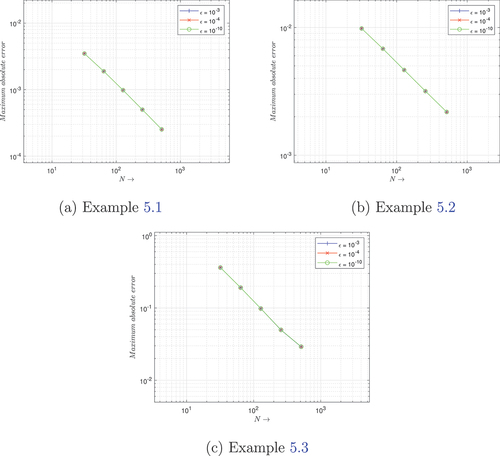
Solution profiles for Examples 5.1, 5.2 and 5.3 are shown in Figures 1, 2 and 3, respectively. In Figure 4, we observe that the behavior of the numerical solution, and for very small values of ɛ, the problem under consideration exhibits an interior layer at s = 1. Figure 5 also shows the log-log plot of the maximum point-wise absolute errors. It confirms the theoretical order of convergence of the suggested numerical scheme. According to the negative slope, the maximum point-wise absolute error decreases with increasing mesh point count. The convergence is parameter-uniform because this behavior is independent of the magnitude of the perturbation parameter applied. One of the primary findings that this paper claims to demonstrate is this.

Figure 1. Numerical solutions of example 5.1 for δ = 0.99 when $\mathit{N}=\mathit{M}=2^6$.

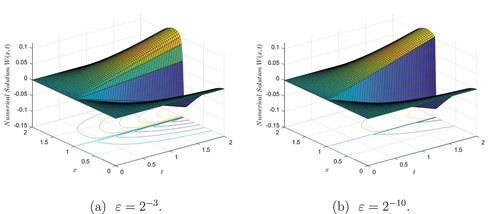
Figure 2. Numerical solutions of example 5.2 for δ = 0.99 when $\mathit{N}=\mathit{M}=2^6$.

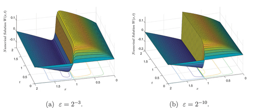
Figure 3. Numerical solutions of example 5.3 for δ = 0.99 when $\mathit{N}=\mathit{M}=2^6$.

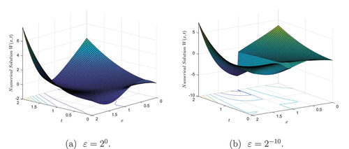
Figure 4. Line graphs at t = 2 when δ = 0.99 and $\mathit{N}=\mathit{M}=2^7$.

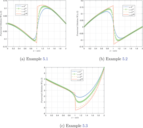
Figure 5. The log-log plot of the maximum absolute errors.

6. Conclusions

A class of SPPDEs with turning point behavior across discontinuities and weak boundary layers is numerically solved in this article. The implicit Euler difference method for the temporal direction and the extended cubic B-spline scheme, containing a free parameter δ for the spatial direction, are used to formulate a parameter-uniform numerical method. The convergence analysis of the method revealed that it is of order $\mathcal{O}(\mathit{k}+\mathbf{h})$, preserving a parameter-uniform convergence. To demonstrate the viability of the suggested method, two examples are taken into consideration for numerical experimentation with different values of $\mathit{\epsilon }$ and number of mesh points. The computational findings are presented in tables and figures. The method improves on the results of certain existing numerical methods in the literature.

Higher-dimensional singularly perturbed parabolic problems can readily be solved using the proposed approach. In subsequent work, we will attempt to broaden the application of the method to semi-linear and higher-dimensional SPPDEs with non-smooth data.

Acknowledgements

The authors would like to express their gratitude to the anonymous referees for their helpful suggestions that helped to improve the quality of this paper.

Disclosure statement

No potential conflict of interest was reported by the author(s).

Funding

This research received no specific funding from public, private, or non-profit funding agencies.

Additional information

Notes on contributors

Wondimagegnehu Simon Hailu

Wondimagegnehu Simon Hailu is a PhD candidate. He is currently employed as a lecturer of mathematics at Dilla University in Ethiopia. His research interest spans the areas of the development of the numerical methods for singularly perturbed ordinary and partial differential equations. He has more than 4 research articles published in various national and international journals.

Gemechis File Duressa

Gemechis File Duressa holds an M.Sc. from Addis Ababa University in Ethiopia and a Ph.D. from the National Institute of Technology in Warangal, India. He is currently employed as a full professor of mathematics and Director of the School of Graduate Studies at Jimma University in Ethiopia. He has over 184 research papers published in various national and international journals. He serves as a referee for several prestigious international journals. He is the research supervisor for Wondimagegnehu Simon Hailu.

References

- Andargie Tiruneh, A., Adamu Derese, G., Amsalu Ayele, M., & Cardone, A. (2023). Singularly perturbed reaction diffusion problem with large spatial delay via non-standard fitted operator method. Research in Mathematics, 10(1), 2171698. https://doi.org/10.1080/27684830.2023.2171698
- Ayele, M. A., Tiruneh, A. A., Derese, G. A., & Araci, S. (2022). Uniformly convergent scheme for singularly perturbed space delay parabolic differential equation with discontinuous convection coefficient and source term. Journal of Mathematics, 2022, 1–15. https://doi.org/10.1155/2022/1874741
- Bansal, K., & Sharma, K. K. (2018). Parameter-robust numerical scheme for time-dependent singularly perturbed reaction–diffusion problem with large delay. Numerical Functional Analysis and Optimization, 39(2), 127–154. https://doi.org/10.1080/01630563.2016.1277742
- Chakravarthy, P. P., Gupta, T., & Rao, N. R. (2018). A numerical scheme for singularly perturbed delay differential equations of convection-diffusion type on an adaptive grid. Mathematical Modelling and Analysis, 23(4), 686–698. https://doi.org/10.3846/mma.2018.041
- Daba, I. T., & Duressa, G. F. (2021). Extended cubic b-spline collocation method for singularly perturbed parabolic differential-difference equation arising in computational neuroscience. International Journal for Numerical Methods in Biomedical Engineering, 37(2), e3418. https://doi.org/10.1002/cnm.3418
- Daba, I. T., & Duressa, G. F. (2022). Computational method for singularly perturbed parabolic differential equations with discontinuous coefficients and large delay. Heliyon, 8(9), e10742. https://doi.org/10.1016/j.heliyon.2022.e10742
- Debela, H. G., & Duressa, G. F. (2020). Accelerated fitted operator finite difference method for singularly perturbed delay differential equations with non-local boundary condition. Journal of the Egyptian Mathematical Society, 28(1), 1–16. https://doi.org/10.1186/s42787-020-00076-6
- Doolan, E. P., Miller, J. J., & Schilders, W. H. (1980). Uniform numerical methods for problems with initial and boundary layers. Boole Press.
- Driver, R. D. (2012). Ordinary and delay differential equations (Vol. 20). Springer Science & Business Media.
- Hailu, W. S., & Duressa, G. F. (2023a). Accelerated parameter-uniform numerical method for singularly perturbed parabolic convection-diffusion problems with a large negative shift and integral boundary condition. Results in Applied Mathematics, 18, 100364. https://doi.org/10.1016/j.rinam.2023.100364
- Hailu, W. S., & Duressa, G. F. (2023b). Uniformly convergent numerical scheme for solving singularly perturbed parabolic convection-diffusion equations with integral boundary condition. Differential Equations and Dynamical Systems, 1–27. https://doi.org/10.1007/s12591-023-00645-y
- Hailu, W. S., Duressa, G. F., & Liu, L. (2022a). Parameter-uniform cubic spline method for singularly perturbed parabolic differential equation with large negative shift and integral boundary condition. Research in Mathematics, 9(1), 2151080. https://doi.org/10.1080/27684830.2022.2151080
- Hailu, W. S., Duressa, G. F., & Liu, L. (2022b). Uniformly convergent numerical method for singularly perturbed parabolic differential equations with non-smooth data and large negative shift. Research in Mathematics, 9(1), 2119677. https://doi.org/10.1080/27684830.2022.2119677
- Hall, C. (1968). On error bounds for spline interpolation. Journal of Approximation Theory, 1(2), 209–218. https://doi.org/10.1016/0021-9045(68)90025-7
- Kaushik, A., & Sharma, N. (2020). An adaptive difference scheme for parabolic delay differential equation with discontinuous coefficients and interior layers. Journal of Difference Equations and Applications, 26(11–12), 1450–1470. https://doi.org/10.1080/10236198.2020.1843645
- Kumar, D., & Kumari, P. (2020). A parameter-uniform scheme for singularly perturbed partial differential equations with a time lag. Numerical Methods for Partial Differential Equations, 36(4), 868–886. https://doi.org/10.1002/num.22455
- Kumar, N. S., & Rao, R. N. (2020). A second order stabilized central difference method for singularly perturbed differential equations with a large negative shift. Differential Equations and Dynamical Systems, 31(4), 1–18. https://doi.org/10.1007/s12591-020-00532-w
- Pramod Chakravarthy, P., Dinesh Kumar, S., & Nageshwar Rao, R. (2017). Numerical solution of second order singularly perturbed delay differential equations via cubic spline in tension. International Journal of Applied and Computational Mathematics, 3(3), 1703–1717. https://doi.org/10.1007/s40819-016-0204-5
- Pramod Chakravarthy, P., Dinesh Kumar, S., Nageshwar Rao, R., & Ghate, D. P. (2015). A fitted numerical scheme for second order singularly perturbed delay differential equations via cubic spline in compression. Advances in Difference Equations, 2015(1), 1–14. https://doi.org/10.1186/s13662-015-0637-x
- Rai, P., & Sharma, K. K. (2020). Numerical approximation for a class of singularly perturbed delay differential equations with boundary and interior layer (s). Numerical Algorithms, 85(1), 305–328. https://doi.org/10.1007/s11075-019-00815-6
- Selvi, P. A., & Ramanujam, N. (2016). An iterative numerical method for singularly perturbed reaction-diffusion equations with negative shift. Journal of Computational and Applied Mathematics, 296, 10–23. https://doi.org/10.1016/j.cam.2015.09.003
- Sharifi, S., & Rashidinia, J. (2019). Collocation method for convection-reaction-diffusion equation. Journal of King Saud University-Science, 31(4), 1115–1121. https://doi.org/10.1016/j.jksus.2018.10.004
- Subburayan, V. (2016). A parameter uniform numerical method for singularly perturbed delay problems with discontinuous convection coefficient. Arab Journal of Mathematical Sciences, 22(2), 191–206. https://doi.org/10.1016/j.ajmsc.2015.07.001
- Subburayan, V. (2018). An hybrid initial value method for singularly perturbed delay differential equations with interior layers and weak boundary layer. Ain Shams Engineering Journal, 9(4), 727–733. https://doi.org/10.1016/j.asej.2016.03.018
- Tian, H. (2002). The exponential asymptotic stability of singularly perturbed delay differential equations with a bounded lag. Journal of Mathematical Analysis and Applications, 270(1), 143–149. https://doi.org/10.1016/S0022-247X(02)00056-2
- Varah, J. M. (1975). A lower bound for the smallest singular value of a matrix. Linear Algebra and Its Applications, 11(1), 3–5. https://doi.org/10.1016/0024-3795(75)90112-3