A new iterative computational scheme for solving second order (1 + 1) boundary value problems with non-homogeneous Dirichlet conditions

ABSTRACT

This paper is a result of an investigation to come up with a new hybrid scheme for solving second order $(1+1)$ boundary value problems of linear as well as nonlinear partial differential equations with non-homogeneous Dirichlet boundary conditions. Such an innovation is significant since there are not many analytical methods for solving partial differential equations with boundary data. The scheme involves the coupling of the ModDTM, a modified form of the Differential Transform Method, and the Adomian Decomposition Method. ModDTM is chosen because the differential transform used in the method is suitable to be applied to boundary value problems. It is the concept of decomposing the initial terms of the series-solution that is borrowed from the Decomposition Method. Solutions are obtained in the form of partial sums of their series representation. These are determined by the application of the mathematical software SageMath. The procedures of application are illustrated by solving linear and nonlinear versions of the classical equations, viz., heat, telegraph, Klein-Gordon and the Fishers equations. To validate the convergence of the solutions obtained with the exact ones two dimensional graphs plotted by SageMath software are used. This is performed in two stages. It is verified that successive partial sums of the series-solutions converge. As well as that, it is shown that the partial sum with the appropriate number of terms converges to the exact and closed form solution. This innovative method is found to be powerful, yet simple and uncomplicated, for solving Dirichlet boundary value problems of second order partial differential equations.

KEYWORDS:

• Boundary value problems
• non-homogeneous dirichlet boundary conditions
• linear and nonlinear partial differential equations
• homogeneous and non-homogeneous partial differential equations
• analytic methods
• Differential transform
• heat equation
• telegraph equation
• Klein-Gordon equation
• fishers equation
• convergence
• 2d-plots

1. Introduction

In this paper, an innovative iterative scheme for solving boundary value problems (BVPs) of partial differential equations (PDEs) is presented. BVPs are typically solved by numerical methods as there are only a few analytical methods that can be applied to them generally. Some examples from literature are the Variational Iteration Method (VIM) (Lu, 2007; Nemrat & Zainuddin, 2020), the Homotopy Analysis Method (HAM) (Nemrat et al., 2019), the Differential Transform Method (DTM) (Al-Ahmad et al., 2022; Al-Rozbayani & Qasim, 2023; Kharrat & Toma, 2020; Mukhtarov et al., 2021) and the Adomian Decomposition Method (ADM) (Adomian & Rach, 1993; Aly et al., 2012; Jang, 2008; Lesnic & Elliott, 1999; Yun et al., 2019), which are seen to be mostly applied for solving such problems of ordinary differential equations (ODEs). For example, in (Lu, 2007) when the VIM is applied to BVPs of ODEs the problem reduces to one of solving systems of algebraic equations. The HAM is coupled with the technique of Sumudu Transform to solve two-point BVPs of linear second order ODEs in (Nemrat et al., 2019). By choosing the initial approximation suitably, the computational procedures are simplified considerably, as claimed by the authors. The DTM is coupled with Laplace transform (LT) and Pad$\stackrel{`}{e}$ approximation for solving ODEs in (Al-Ahmad et al., 2022). Solutions obtained are shown to be better approximations than those obtained by the application of the DTM directly, or the ADM. Systems of fourth order ODEs with Dirichlet BCs are solved in (Kharrat & Toma, 2020) by combining DTM with Maple. A new version of the method called the α-parameterized DTM, which is a generalized form of the method, is applied in (Mukhtarov et al., 2021) for solving ODEs, and in (Al-Rozbayani & Qasim, 2023) for the nonlinear Gardner equation. α is a parameter in (0, 1) using which a convex function is constructed. It is the optimal value of α, determined by applying a genetic algorithm (Al-Rozbayani & Qasim, 2023), that generates the best possible approximation of the solution-function. The method is felt to be computationally very involved. Adaptations and modifications of ADM for solving BVPs are found in (Adomian & Rach, 1993; Aly et al., 2012; Jang, 2008; Lesnic & Elliott, 1999; Yun et al., 2019). For example, BVPs of second order PDEs with non-homogeneous Dirichlet BCs on triangular areas are solved by a segmented version of the ADM in (Yun et al., 2019). The triangular domain of application is segmented further into more of them by redefining boundaries, and new BCs are defined. Recurrence relations involving double integrals are then used to determine the solutions as applicable to the various triangular segments. The method is innovative, yet very involved.

In this study, a new scheme is devised by combining concepts of two of these methods, namely, the DTM and the ADM, for solving PDEs for which non-homogeneous Dirichlet boundary conditions (BC) have been prescribed. The DTM was first devised in 1986 by Zhou who applied it for solving PDEs in electric circuit analysis, as mentioned in (Chen & Ho, 1999). What is being proposed in the present work is a hybridization of a modified form of the DTM, and the Decomposition method of Adomian. The modification identified for the purpose is the ModDTM, which was first devised by the authors of this paper in (Nayar & Phiri, 2020). It was devised for solving $(1+1)$ linear and nonlinear PDEs with search direction of the solution along the spatial axis. As such, solutions obtained are in the form of a power series in x. For this reason, the ModDTM is suitable for BVPs as boundary conditions may be applied directly to the solution. The modified differential transform (Mod DT) (Nayar & Phiri, 2020) that forms the basis of the ModDTM is the first component in the hybridization, as it is used to determine a recurrence relation as a first step. This relation has two initial terms since the equations solved are of order two. The first one of these terms will be provided by the first boundary condition. But, the second initial term cannot be determined directly as the data available is a BC. This is where the concept of decomposition of the initial terms of the series-solution is applied. In (Adomian & Rach, 1993), Adomian outlines a scheme for solving second order BVPs with non-homogeneous two-point boundary conditions (BCs). The highlight of the method is the decomposition of the initial terms. A similar technique is proposed to be used to find the second initial term in the new method. The solutions obtained will be in the form of successive partial sums S_n of their series representation, which are expected to converge to each other after a finitely small number of iterations, and they, to the exact and closed-form solution of the PDE. Comparison of 2d graphs of the obtained solutions with those of the exact ones will be carried out to show such convergence technically. The graphs will be plotted using SageMath. From hereon, the new method will be referred to as the New Modified Differential Transform-Decomposition method (NMDT-D), as it combines concepts of the ModDTM and the ADM. In order to examine the applicability and effectiveness of the method, it is tested on some $(1+1)$ second order PDEs with non-homogeneous Dirichlet BCs for which solutions are available. These include linear, nonlinear, homogeneous and non-homogeneous versions of the classical heat, telegraph, Klein-Gordon (KG) and Fishers equations.

The paper is set as follows. In section 2 detailed description of the new method is presented by discussing its various procedural aspects. Section 3 contains examples of application of the NMDT-D for solving the PDEs. Results and Discussion are included in Section 4. Finally, Section 5 concludes the paper.

2. Description of the method

As the first procedure in the application of NMDT-D method involves the utilization of concepts of ModDTM, it is felt that these should be explained briefly before presenting the particulars of the new method.

2.1. The ModDTM

The ModDTM may be said to be an improvement of the DTM (Al-Ahmad et al., 2022; Al-Rozbayani & Qasim, 2023; Kharrat & Toma, 2020; Mukhtarov et al., 2021). The key element of the method is the differential transform used in its application. The k-th transform of a function $\mathit{u}(\mathit{x},\mathit{t})$ is defined as (Nayar & Phiri, 2020)

(1) $\begin{array}{l}{U}_k\left(\mathit{t}\right)=\frac{1}{\mathit{k}!}{\left[\frac{{\mathit{\partial }}^{\mathit{k}}\mathit{u}}{\mathit{\partial }{x}^k}\right]}_{\mathit{x}=0},\end{array}$(1)

and the inverse transform as (Nayar & Phiri, 2020)

(2) $\begin{array}{l}\mathit{u}(\mathit{x},\mathit{t})=\sum _{\mathit{k}=0}^{\mathrm{\infty }}{U}_k\left(\mathit{t}\right)x^k=\sum _{\mathit{k}=0}^{\mathrm{\infty }}\frac{1}{\mathit{k}!}{\left[\frac{{\mathit{\partial }}^{\mathit{k}}\mathit{u}}{\mathit{\partial }{x}^k}\right]}_{\mathit{x}=0}{x}^k.\end{array}$(2)

To solve a PDE by the method, the equation is first converted to a recurrence relation by applying the transform and its various properties that may be referenced in (Nayar & Phiri, 2020). This relation is then used recursively to determine the coefficients $U_k(\mathit{t})$ of the corresponding series representation of the solution function $\mathit{u}(\mathit{x},\mathit{t})$ as in (Equation 2(2) $\begin{array}{l}\mathit{u}(\mathit{x},\mathit{t})=\sum _{\mathit{k}=0}^{\mathrm{\infty }}{U}_k\left(\mathit{t}\right)x^k=\sum _{\mathit{k}=0}^{\mathrm{\infty }}\frac{1}{\mathit{k}!}{\left[\frac{{\mathit{\partial }}^{\mathit{k}}\mathit{u}}{\mathit{\partial }{x}^k}\right]}_{\mathit{x}=0}{x}^k.\end{array}$(2) ) (Nayar & Phiri, 2020). Below is given a symbolic derivation of the recurrence relation.

Consider the general $(1+1)$ second order PDE represented by

(3) $\begin{array}{l}\mathit{L}(\mathit{u})+\mathit{R}(\mathit{u})+\mathit{N}(\mathit{u})=\mathit{f}(\mathit{x},\mathit{t}),\end{array}$(3)

where L(u) represents the linear second order partial differential operator, N(u) is a nonlinear operator such as u² or sin(u) or e^u, and R(u) represents the remaining operators in the equation. $\mathit{f}(\mathit{x},\mathit{t})$ is a forcing term. The terms of (Equation 3(3) $\begin{array}{l}\mathit{L}(\mathit{u})+\mathit{R}(\mathit{u})+\mathit{N}(\mathit{u})=\mathit{f}(\mathit{x},\mathit{t}),\end{array}$(3) ) are rearranged to obtain:

$\begin{array}{l}\mathit{L}(\mathit{u})=\mathit{f}(\mathit{x},\mathit{t})-\mathit{R}(\mathit{u})-\mathit{N}(\mathit{u}).\end{array}$

Inverting L:

(4) $\begin{array}{ll}\mathit{u}& =L^{-1}(\mathit{f}(\mathit{x},\mathit{t})-\mathit{R}(\mathit{u})-\mathit{N}(\mathit{u}))\\ & =c_0(\mathit{t})+\mathit{x}{c}_1(\mathit{t})+\int \int (\mathit{f}(\mathit{x},\mathit{t})-\mathit{R}(\mathit{u})-\mathit{N}(\mathit{u}))\mathit{dxdx},\end{array}$(4)

where $c_0(\mathit{t})=\mathit{u}(0,\mathit{t})$ and $c_1(\mathit{t})=u_{\mathit{x}}(0,\mathit{t})$ are the initial conditions (ICs) with respect to x. The integral therefore represents indefinite integration. Suppose F_k, R_k and N_k represent the kth Mod DT of $\mathit{f}(\mathit{x},\mathit{t})$, R(u) and N(u), respectively. Then using (Equation 2(2) $\begin{array}{l}\mathit{u}(\mathit{x},\mathit{t})=\sum _{\mathit{k}=0}^{\mathrm{\infty }}{U}_k\left(\mathit{t}\right)x^k=\sum _{\mathit{k}=0}^{\mathrm{\infty }}\frac{1}{\mathit{k}!}{\left[\frac{{\mathit{\partial }}^{\mathit{k}}\mathit{u}}{\mathit{\partial }{x}^k}\right]}_{\mathit{x}=0}{x}^k.\end{array}$(2) ),

(5) $\begin{array}{ll}\sum _{\mathit{k}=0}^{\mathrm{\infty }}& U_{\mathit{k}}\left(\mathit{t}\right)x^{\mathit{k}}\\ & =\int \int \left\{\sum _{\mathit{k}=0}^{\mathrm{\infty }}[F_{\mathit{k}}\left(\mathit{t}\right)x^{\mathit{k}}-R_{\mathit{k}}\left(\mathit{t}\right)x^{\mathit{k}}-N_{\mathit{k}}\left(\mathit{t}\right)x^{\mathit{k}}]\right\}\mathit{dxdx}\\ & +c_0\left(\mathit{t}\right)+\mathit{x}{c}_1\left(\mathit{t}\right)\\ & =\sum _{\mathit{k}=0}^{\mathrm{\infty }}[F_{\mathit{k}}\left(\mathit{t}\right)-R_{\mathit{k}}\left(\mathit{t}\right)-N_{\mathit{k}}\left(\mathit{t}\right)]\frac{x^{\mathit{k}+2}}{(\mathit{k}+1)(\mathit{k}+2)}\\ & +c_0\left(\mathit{t}\right)+\mathit{x}{c}_1\left(\mathit{t}\right)\\ & =\sum _{\mathit{k}=2}^{\mathrm{\infty }}[F_{\mathit{k}-2}\left(\mathit{t}\right)-R_{\mathit{k}-2}\left(\mathit{t}\right)-N_{\mathit{k}-2}\left(\mathit{t}\right)]\frac{x^{\mathit{k}}}{(\mathit{k}-1)\left(\mathit{k}\right)}\\ & +c_0\left(\mathit{t}\right)+\mathit{x}{c}_1\left(\mathit{t}\right).\end{array}$(5)

Equating coefficients, $c_0(\mathit{t})=\mathit{u}(0,\mathit{t})=U_0(\mathit{t})$ and $c_1(\mathit{t})=u_x(0,\mathit{t})=U_1(\mathit{t})$. The coefficients for $\mathit{k}\ge 2$ are given by

(6) $U_{\mathit{k}}\left(\mathit{t}\right)=\frac{1}{\mathit{k}(\mathit{k}-1)}[F_{\mathit{k}-2}\left(\mathit{t}\right)-R_{\mathit{k}-2}\left(\mathit{t}\right)-N_{\mathit{k}-2}\left(\mathit{t}\right)].$(6)

(Equation 6(6) $U_{\mathit{k}}\left(\mathit{t}\right)=\frac{1}{\mathit{k}(\mathit{k}-1)}[F_{\mathit{k}-2}\left(\mathit{t}\right)-R_{\mathit{k}-2}\left(\mathit{t}\right)-N_{\mathit{k}-2}\left(\mathit{t}\right)].$(6) is the recurrence relation, which determines the coefficients in the power series solution for $\mathit{k}\ge 2$. In (Nayar & Phiri, 2020) the ModDTM has been successfully applied to solve several nonlinear PDEs. The reader may refer to the work for a better picture of the application procedure of the method.

2.2. The new modified differential transform-decomposition method

In the application of NMDT-D, $c_1(\mathit{t})$ is not known, since the PDE is prescribed BCs instead of ICs. Hence, a plan different from that of the ModDTM is required for determining the solution of (Equation 3(3) $\begin{array}{l}\mathit{L}(\mathit{u})+\mathit{R}(\mathit{u})+\mathit{N}(\mathit{u})=\mathit{f}(\mathit{x},\mathit{t}),\end{array}$(3) ). This is where the ADM comes in. In an approach suggested by Adomian in (Adomian & Rach, 1993), the initial terms $c_0(\mathit{t})$ and $c_1(\mathit{t})$ are decomposed. Applying a similar technique (Equation 6(6) $U_{\mathit{k}}\left(\mathit{t}\right)=\frac{1}{\mathit{k}(\mathit{k}-1)}[F_{\mathit{k}-2}\left(\mathit{t}\right)-R_{\mathit{k}-2}\left(\mathit{t}\right)-N_{\mathit{k}-2}\left(\mathit{t}\right)].$(6) ) may be rewritten as

(7) $\begin{array}{ll}\sum _{\mathit{k}=0}^{\mathrm{\infty }}{U}_{\mathit{k}}\left(\mathit{t}\right)x^{\mathit{k}}& =\sum _{\mathit{k}=2}^{\mathrm{\infty }}[F_{\mathit{k}-2}\left(\mathit{t}\right)-R_{\mathit{k}-2}\left(\mathit{t}\right)-N_{\mathit{k}-2}\left(\mathit{t}\right)]\frac{x^{\mathit{k}}}{(\mathit{k}-1)\left(\mathit{k}\right)}\\ & +\sum _{\mathit{k}=0}^{\mathrm{\infty }}{c}_{0,\mathit{k}}+\mathit{x}\sum _{\mathit{k}=0}^{\mathrm{\infty }}{c}_{1,\mathit{k}},\end{array}$(7)

by decomposing each one of $c_0(\mathit{t})$ and $c_1(\mathit{t})$ to an infinite sum. Such a decomposition is possible since a double integration is performed to determine $U_k(\mathit{t})$ for each k, at least symbolically.

The next step in the plan is to set up recurrence relations using (Equation 7(7) $\begin{array}{ll}\sum _{\mathit{k}=0}^{\mathrm{\infty }}{U}_{\mathit{k}}\left(\mathit{t}\right)x^{\mathit{k}}& =\sum _{\mathit{k}=2}^{\mathrm{\infty }}[F_{\mathit{k}-2}\left(\mathit{t}\right)-R_{\mathit{k}-2}\left(\mathit{t}\right)-N_{\mathit{k}-2}\left(\mathit{t}\right)]\frac{x^{\mathit{k}}}{(\mathit{k}-1)\left(\mathit{k}\right)}\\ & +\sum _{\mathit{k}=0}^{\mathrm{\infty }}{c}_{0,\mathit{k}}+\mathit{x}\sum _{\mathit{k}=0}^{\mathrm{\infty }}{c}_{1,\mathit{k}},\end{array}$(7) ). The process is initialized by defining the first term of the series $\sum _{\mathit{k}}{u}_k$ as

$\begin{array}{l}{u}_0=c_{0,0}+\mathit{x}{c}_{1,0}.\end{array}$

Suppose S_n represents the n-th partial sum of the series solution. Then, equating the first partial sum to u₀:

$\begin{array}{l}{S}_1=c_{0,0}+\mathit{x}{c}_{1,0}.\end{array}$

As S₁ may be considered to be the first approximation of $\mathit{u}(\mathit{x},\mathit{t})$, it should satisfy the prescribed BCs. Applying these conditions, one obtains the unknowns $c_{0,0}$ and $c_{1,0}$, which determine S₁. Next, set

$\begin{array}{l}{u}_1=c_{0,1}+\mathit{x}{c}_{1,1}+(F_0-R_0-N_0)\frac{x^2}{2}.\end{array}$

u₁ is the second term in the series, so that the next partial sum is obtained as

$\begin{array}{l}{S}_2=S_1+u_1=S_1+c_{0,1}+\mathit{x}{c}_{1,1}+(F_0-R_0-N_0)\frac{x^2}{2}.\end{array}$

In this formula, $F_0=\mathit{f}(0,\mathit{t})$, $R_0=\mathit{R}(\mathit{u}){|}_{\mathit{x}=0}$ and $N_0=\mathit{N}(\mathit{u}){|}_{\mathit{x}=0}$. Since u is unknown, it is replaced by S₁, its first approximation. Thus

$\begin{array}{l}{R}_0=\mathit{R}(S_1){|}_{\mathit{x}=0},N_0=\mathit{N}(S_1){|}_{\mathit{x}=0}.\end{array}$

Hence

(8) $\begin{array}{l}{S}_2=S_1+c_{0,1}+\mathit{x}{c}_{1,1}+(F_0-R_0(S_1)-N_0(S_1))\frac{x^2}{2}.\end{array}$(8)

Once again the BCs are applied to (Equation 8(8) $\begin{array}{l}{S}_2=S_1+c_{0,1}+\mathit{x}{c}_{1,1}+(F_0-R_0(S_1)-N_0(S_1))\frac{x^2}{2}.\end{array}$(8) ) to find $c_{0,1}$ and $c_{1,1}$, thereby determining S₂. The procedures are repeated to determine the successive partial sums, until satisfactory levels of convergence is reached. Thus, it may well be said that two recurrence relations sum up the procedures of the NMDT-D method. These are

(9) $\begin{array}{l}{u}_{\mathit{k}}=c_{0,\mathit{k}}+\mathit{x}{c}_{1,\mathit{k}}+(F_{\mathit{k}-1}-R_{\mathit{k}-1}(S_k)-N_{\mathit{k}-1}(S_k))\frac{x^{\mathit{k}+1}}{(\mathit{k})(\mathit{k}+1)},\end{array}$(9)

for $\mathit{k}\ge 0$, with $F_{-1}=R_{-1}=N_{-1}=0$, and

(10) $\begin{array}{l}{S}_{\mathit{k}+1}=S_{\mathit{k}}+u_{\mathit{k}},S_0=0,\end{array}$(10)

where

$\begin{array}{ll}{R}_{\mathit{k}-1}(S_k)& =\frac{1}{(\mathit{k}-1)!}\left(\frac{{\mathit{\partial }}^{\mathit{k}-1}\mathit{R}(S_k)}{\mathit{\partial }{x}^{\mathit{k}-1}}\right),\\ N_{\mathit{k}-1}(S_k)& =\frac{1}{(\mathit{k}-1)!}\left(\frac{{\mathit{\partial }}^{\mathit{k}-1}\mathit{N}(S_k)}{\mathit{\partial }{x}^{\mathit{k}-1}}\right)\end{array}$

and

$\begin{array}{l}{F}_{\mathit{k}-1}(S_k)=\frac{1}{(\mathit{k}-1)!}\left(\frac{{\mathit{\partial }}^{\mathit{k}-1}\mathit{f}(\mathit{x},\mathit{t})}{\mathit{\partial }{x}^{\mathit{k}-1}}\right),\end{array}$

are evaluated at x = 0.

3. Convergence analysis of the NMDT-D method

The Banach Fixed Point Theorem (Kreyszig, 1991) is applied to analyze the convergence of the solutions generated by the method. As per the theorem, if T is a contraction mapping defined on a Banach space X, then T has a unique fixed point in X.

3.1. Theorem

Consider the Banach space of continuous functions C in $\mathrm{\Omega }=[\mathit{a},\mathit{b}]\times [\mathit{c},\mathit{d}]$ with an appropriate norm. Let $B_r(\mathit{u})=\{S_n\mathit{ϵ}\mathrm{\Omega }|\Vert S_n-\mathit{u}\Vert <\mathit{r}\}$, where $\mathit{u}(\mathit{x},\mathit{t})$ is the solution of the PDE. S_n denotes the partial sum of the infinite series $\sum _{\mathit{k}=0}^{\mathrm{\infty }}{u}_k$, and r > 0 is a constant. Then, the series converges if there exists an $\mathit{\alpha ϵ}(0,1)$ such that $\Vert u_{\mathit{n}+1}\Vert \le \mathit{\alpha }\Vert u_{\mathit{n}}\Vert$.

Proof.

Starting with $u_0\mathit{ϵ}{B}_r(\mathit{u})$, define the mapping $\mathit{T}(S_n)=S_{\mathit{n}+1},\mathit{n}=1,2,3,\cdots .$ Then,

(11) $\begin{array}{ll}\Vert \mathit{T}(S_n)-\mathit{T}(S_{\mathit{n}-1})\Vert & =\Vert S_{\mathit{n}+1}-S_n\Vert =\Vert u_n\Vert \le \mathit{\alpha }\Vert u_{\mathit{n}-1}\Vert \\ & \le {\alpha }^2\Vert u_{\mathit{n}-2}\Vert \le {\alpha }^3\Vert u_{\mathit{n}-3}\Vert \le \cdots \\ & \le {\alpha }^n\Vert u_0\Vert .\end{array}$(11)

Successive application of (Equation 11(11) $\begin{array}{ll}\Vert \mathit{T}(S_n)-\mathit{T}(S_{\mathit{n}-1})\Vert & =\Vert S_{\mathit{n}+1}-S_n\Vert =\Vert u_n\Vert \le \mathit{\alpha }\Vert u_{\mathit{n}-1}\Vert \\ & \le {\alpha }^2\Vert u_{\mathit{n}-2}\Vert \le {\alpha }^3\Vert u_{\mathit{n}-3}\Vert \le \cdots \\ & \le {\alpha }^n\Vert u_0\Vert .\end{array}$(11) ) shows that $\{\mathit{T}(S_n)\}$ is a Cauchy sequence.

$\begin{array}{ll}\Vert \mathit{T}(S_n)& -\mathit{T}(S_m)\Vert \\ & =\Vert \mathit{T}(S_n)-\mathit{T}(S_{\mathit{n}-1})+\mathit{T}(S_{\mathit{n}-1})-\cdots +\mathit{T}(S_{\mathit{m}+1})-\mathit{T}(S_m)\Vert \\ & \le \Vert \mathit{T}(S_n)-\mathit{T}(S_{\mathit{n}-1})\Vert +\Vert \mathit{T}(S_{\mathit{n}-1})-\mathit{T}(S_{\mathit{n}-2})\Vert +\cdots \\ & +\Vert \mathit{T}(S_{\mathit{m}+1})-\mathit{T}(S_m)\Vert \\ & \le {\alpha }^n\Vert u_0\Vert +{\alpha }^{\mathit{n}-1}\Vert u_0\Vert +{\alpha }^{\mathit{n}-2}\Vert u_0\Vert +\cdots +{\alpha }^{\mathit{m}+1}\Vert u_0\Vert \\ & \le {\alpha }^{\mathit{m}+1}(1+\mathit{\alpha }+{\alpha }^2+\cdots +{\alpha }^{\mathit{n}-\mathit{m}-1})\Vert u_0\Vert \\ & \le {\alpha }^{\mathit{m}+1}\left(\frac{1-{\mathit{\alpha }}^{\mathit{n}-\mathit{m}}}{1-\mathit{\alpha }}\right)\Vert u_0\Vert \le \left(\frac{{\alpha }^{\mathit{m}+1}}{1-\mathit{\alpha }}\right)\Vert u_0\Vert ,\end{array}$

since $1-{\alpha }^{\mathit{n}-\mathit{m}}<1$ as $0<\mathit{\alpha }<1$. Since $\{\mathit{T}(S_n)\}$ is a Cauchy sequence in a complete space, it should converge to a unique fixed point, say, S such that $\mathit{T}(\mathit{S})=\mathit{S}=\sum u_k.$

4. Numerical examples

In this section, the application of NMDT-D is illustrated by applying the method to cases of homogeneous and non-homogeneous versions of linear and nonlinear classical PDEs, such as the heat, telegraph, Klein-Gordon and Fisher equations. The procedures followed for solving the equations are explained in Section 2.2.

4.1. Linear and homogeneous heat equation

The heat equation is fundamental in modeling several kinds of diffusion processes occurring in physics, chemistry, and the biological sciences. The equation considered is (2012)

(12) $\begin{array}{l}{u}_t=u_{\mathit{xx}},0\le \mathit{x}\le 1,\mathit{t}\ge 0,\end{array}$(12)

and is prescribed the BCs

$\begin{array}{l}\mathit{u}(0,\mathit{t})=e^t,\mathit{u}(1,\mathit{t})=e^t\mathit{cosh}(1).\end{array}$

This being a linear and homogeneous PDE, $\mathit{N}(\mathit{u})=0$ and $\mathit{f}(\mathit{x},\mathit{t})=0$. The other operators occurring in the equation are $\mathit{L}(\mathit{u})=u_{\mathit{xx}}$ are $\mathit{R}(\mathit{u})=u_t$. Recurrence relations given by (Equation 9(9) $\begin{array}{l}{u}_{\mathit{k}}=c_{0,\mathit{k}}+\mathit{x}{c}_{1,\mathit{k}}+(F_{\mathit{k}-1}-R_{\mathit{k}-1}(S_k)-N_{\mathit{k}-1}(S_k))\frac{x^{\mathit{k}+1}}{(\mathit{k})(\mathit{k}+1)},\end{array}$(9) ) and (Equation 10(10) $\begin{array}{l}{S}_{\mathit{k}+1}=S_{\mathit{k}}+u_{\mathit{k}},S_0=0,\end{array}$(10) ) will be applied recursively to solve the given equation. Start by setting

$\begin{array}{l}{u}_0=c_{0,0}+\mathit{x}{c}_{1,0}.\end{array}$

The first partial sum is then set as

(13) $\begin{array}{l}{S}_1=c_{0,0}+\mathit{x}{c}_{1,0}.\end{array}$(13)

Setting x = 0 and x = 1 in (Equation 13(13) $\begin{array}{l}{S}_1=c_{0,0}+\mathit{x}{c}_{1,0}.\end{array}$(13) ), and solving the equations so obtained $c_{0,0}$ and $c_{1,0}$ are found to be

$\begin{array}{l}{c}_{0,0}=e^t,c_{1,0}=e^t(\mathit{cosh}(1)-1).\end{array}$

Thus

$\begin{array}{l}{S}_1=e^t[1+\mathit{x}(\mathit{cosh}(1)-1)].\end{array}$

Next set

$\begin{array}{l}{u}_1=c_{0,1}+\mathit{x}{c}_{1,1}+(R_0(S_1))\frac{x^2}{2}.\end{array}$

The second partial sum is

$\begin{array}{l}{S}_2=S_1+c_{0,1}+\mathit{x}{c}_{1,1}+(R_0(S_1))\frac{x^2}{2}.\end{array}$

$\begin{array}{l}{R}_0(S_1)={[R(S_1)]}_{\mathit{x}=0}={\left[\frac{\partial S_1}{\mathit{\partial t}}\right]}_{\mathit{x}=0}=e^t.\end{array}$

Hence

$\begin{array}{ll}{S}_2& =e^t[1+\mathit{x}(\mathit{cosh}(1)-1)]+c_{0,1}+\mathit{x}{c}_{1,1}+e^t\left(\frac{x^2}{2}\right)\\ & =c_{0,1}+\mathit{x}{c}_{1,1}+e^t[1+\mathit{x}(\mathit{cosh}(1)-1)+\frac{x^2}{2}].\end{array}$

BCs are applied to S₂ to obtain $c_{0,1}=0$ and $c_{1,1}=-\frac{e^t}{2}$. Thereby

$\begin{array}{l}{S}_2=e^t(1+\mathit{x}(\mathit{cosh}(1)-\frac{3}{2})+\frac{x^2}{2}).\end{array}$

The processes are repeated to get

$\begin{array}{ll}{S}_3& =e^t(1+\frac{5\mathit{x}}{6}(\mathit{cosh}(1)-\frac{3}{2})+\frac{x^2}{2}\\ & +(\mathit{cosh}(1)-\frac{3}{2})\frac{x^3}{6});\end{array}$

$\begin{array}{ll}{S}_4& =e^t(1+(\frac{5}{6}\mathit{cosh}(1)-\frac{31}{24})\mathit{x}+\frac{x^2}{2}\\ & +(\mathit{cosh}(1)-\frac{3}{2})\frac{x^3}{6}+\frac{x^4}{24});\end{array}$

$\begin{array}{ll}{S}_5& =e^t(1+(\frac{33}{40}\mathit{cosh}(1)-\frac{307}{240})\mathit{x}+\frac{x^2}{2}\\ & +(\mathit{cosh}(1)-\frac{3}{2})\frac{x^3}{6}+\frac{x^4}{24})\\ & +e^t\left((\mathit{cosh}(1)-\frac{3}{2})\frac{x^5}{120}\right);\end{array}$

$\begin{array}{ll}{S}_6& =e^t(1+(\frac{33}{40}\mathit{cosh}(1)-\frac{461}{360})\mathit{x}+\frac{x^2}{2}\\ & +(\mathit{cosh}(1)-\frac{3}{2})\frac{x^3}{6}+\frac{x^4}{24})\\ & +e^t((\mathit{cosh}(1)-\frac{3}{2})\frac{x^5}{120}+\frac{x^6}{720});\end{array}$

$\begin{array}{ll}{S}_7& =e^t(1+(\frac{4157}{5040}\mathit{cosh}(1)-\frac{2581}{2016})\mathit{x}+\frac{x^2}{2}\\ & +(\mathit{cosh}(1)-\frac{3}{2})\frac{x^3}{6}+\frac{x^4}{24})\\ & +e^t((\mathit{cosh}(1)-\frac{3}{2})\frac{x^5}{120}+\frac{x^6}{720}\\ & +(\mathit{cosh}(1)-\frac{3}{2})\frac{x^7}{5040}).\end{array}$

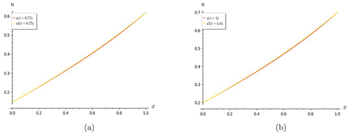
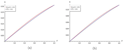
The graphs in Figures 1 and 2 compares $S_7(\mathit{x},\mathit{t})$ with the exact solution $\mathit{u}(\mathit{x},\mathit{t})=e^t\mathit{cosh}\mathit{x}$ (2012). It is seen that S₇ is a good approximation of u. The other graphs in Figures 2 and 3 indicate that even S₅ is a good approximation, since S₇ converges well with both S₅ and S₆ .

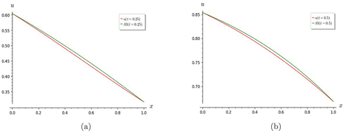
Figure 1. Graphs of heat equation. S₇ shows good convergence with the exact solution for (a) t = 0 and (b) t = 0.5.

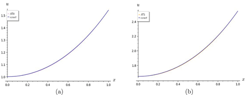
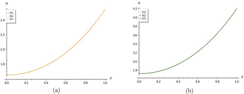
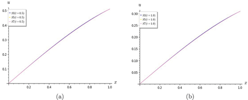
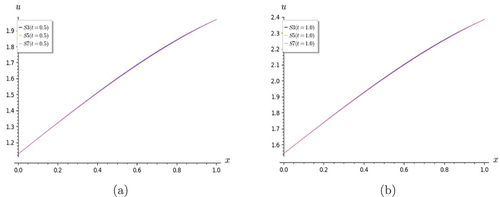
Figure 2. Graphs of heat equation. (a) shows S₇ converges well with exact solution for t = 1. (b) figure shows convergence of partial sums S₅, S₆ and S₇ for t = 0.

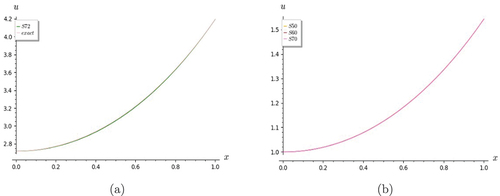
Figure 3. Graphs of heat equation. Figure shows convergence of partial sums for (a) $\mathit{t}=0.5,\mathit{and}(\mathit{b})\mathit{t}=1.$

4.2. Linear and homogeneous telegraph equation

The telegraph equation, which was first designed to deal with electrical circuit problems, has recently been the subject of intense research for its myriad applications in the communication field, as it is specified in (Hussen et al., 2022; Lock et al., 2007) and in the references therein. The equation considered is another linear and homogeneous PDE defined in $[0,1]\times [0,\mathrm{\infty }]$, and it takes the form (Soltanalizadeh, 2011):

(14) $\begin{array}{ll}& u_{\mathit{xx}}=u_{\mathit{tt}}+u_{\mathit{t}}-\mathit{u},\mathit{u}(0,\mathit{t})=0,\\ & \mathit{u}(1,\mathit{t})=\mathit{sin}(1)e^{-\mathit{t}},\mathit{u}(\mathit{x},0)=\mathit{sin}\mathit{x}.\end{array}$(14)

In the equation, $\mathit{L}(\mathit{u})=u_{\mathit{xx}}$ and $\mathit{R}(\mathit{u})=u_{\mathit{tt}}+u_{\mathit{t}}-\mathit{u}$. The exact and closed form solution is $\mathit{u}(\mathit{x},\mathit{t})=e^{-\mathit{t}}\mathit{sin}\mathit{x}$ (Soltanalizadeh, 2011). Following the procedures of the method as illustrated in the previous example, the first seven partial sums are determined as given below.

$\begin{array}{l}{S}_1=S_2=\mathit{sin}(1)e^{-\mathit{t}}\mathit{x};\end{array}$

$\begin{array}{l}{S}_3=S_4=\mathit{sin}(1)e^{-\mathit{t}}((1+\frac{1}{3!})\mathit{x}-\frac{x^3}{3!});\end{array}$

$\begin{array}{l}{S}_5=S_6=\mathit{sin}(1)e^{-\mathit{t}}((1+\frac{1}{3!}-\frac{1}{5!})\mathit{x}-\frac{x^3}{3!}+\frac{x^5}{5!});\end{array}$

$\begin{array}{l}{S}_7=\mathit{sin}(1)e^{-\mathit{t}}((1+\frac{1}{3!}-\frac{1}{5!}+\frac{1}{7!})\mathit{x}-\frac{x^3}{3!}+\frac{x^5}{5!}-\frac{x^7}{7!}),\end{array}$

since $u_1=u_3=u_5=0$. In fact, the pattern seen in the form of the partial sums allows the generalization:

$\begin{array}{l}{S}_{\mathrm{\infty }}=\mathit{sin}(1)e^{-\mathit{t}}((1-\mathit{sin}(1))\mathit{x}+\mathit{sin}\mathit{x}).\end{array}$

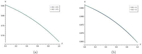
Table 1 allows a comparison to be made between the exact solution and $S_{\mathrm{\infty }}$. In the table, the first row gives the exact solution, whereas the second row represents the values of $S_{\mathrm{\infty }}$ for each value of x. The good agreement that the latter has with the former is evident, especially as t is increased. Some graphs are also included (Figures 4-6). From the graphs, it is understood that even though S₇ approximates the exact solution very well, convergence is reached even as early as S₃, since S₃, S₅ and S₇ are in good agreement.

Table 1. Linear and homogeneous telegraph equation

x	t=0.0	t=0.5	t=1.0	t=2.0
0.0	0.00	0.00	0.00	0.00
	0.00	0.00	0.00	0.00
0.2	0.19866933	0.120499040	0.073086362	0.026886970
	0.19385399	0.117578388	0.071314897	0.026235284
0.5	0.479425538	0.290786288	0.176370799	0.064883190
	0.470121463	0.285143081	0.172948021	0.063624021
0.8	0.717356090	0.435098462	0.263900557	0.097083589
	0.710352389	0.430850503	0.261324039	0.096135741
1.0	0.841470984	0.510377951	0.309559875	0.113880714
	0.841770984	0.510377951	0.309559875	0.113880714

Figure 4. Graphs of Lin and Hom Telegraph Equation. S₇ shows a good rate of convergence with the exact solution for (a) t = 0 and (b) t = 0.5.

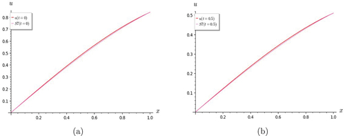
Figure 5. Graphs of Lin and Hom Telegraph Equation. (a) S₇ shows good convergence with the exact solution for t = 1.0; (b) the partial sums S₃, S₅ and S₇ are in good agreement for t = 0.

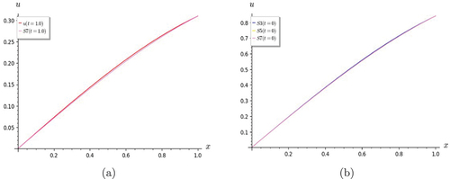
Figure 6. Graphs of Lin and Hom Telegraph Equation. The partial sums S₃, S₅ and S₇ are in good agreement for (a) t = 0.5 and (b) t= 1.

4.3. Linear and homogeneous Klein-Gordon equation

A homogeneous version of the linear Klein-Gordon equation (K-G) defined for $0\le \mathit{x}\le 1$ and $\mathit{t}\ge 0$ is given by (Ahmad et al., 2015)

(15) $\begin{array}{l}{u}_{\mathit{xx}}=u_{\mathit{tt}}-\mathit{u}.\end{array}$(15)

The BCs obtained from the exact solution $\mathit{u}(\mathit{x},\mathit{t})=\mathit{sin}\mathit{x}+\mathit{cosh}\mathit{t}$ (Ahmad et al., 2015) of (Equation 15(15) $\begin{array}{l}{u}_{\mathit{xx}}=u_{\mathit{tt}}-\mathit{u}.\end{array}$(15) ) are

$\begin{array}{l}\mathit{u}(0,\mathit{t})=\mathit{cosh}\mathit{t},\mathit{u}(1,\mathit{t})=\mathit{cosh}\mathit{t}+\mathit{sin}1.\end{array}$

Applying the NMDT-D, partial sums are obtained as given below.

$\begin{array}{l}{S}_1=S_2=\mathit{cosh}\mathit{t}+(\mathit{sin}1)\mathit{x};\end{array}$

$\begin{array}{l}{S}_3=S_4=\mathit{cosh}\mathit{t}+(\mathit{sin}1)(\frac{7\mathit{x}}{6}-\frac{x^3}{3!});\end{array}$

$\begin{array}{l}{S}_5=S_6=\mathit{cosh}\mathit{t}+(\mathit{sin}1)(\frac{139\mathit{x}}{120}-\frac{x^3}{3!}+\frac{x^5}{5!});\end{array}$

$\begin{array}{l}{S}_7=\mathit{cosh}\mathit{t}+(\mathit{sin}1)(\frac{5839\mathit{x}}{5040}-\frac{x^3}{3!}+\frac{x^5}{5!}-\frac{x^7}{7!}),\end{array}$

since $u_1=u_3=u_5=0$. Figures 7–9 show the good agreement of the computed solution with the exact one. As in the case of the linear and homogeneous telegraph equation, the solution may be considered to be S₃, as S₅ and S₇ show convergence with it.

Figure 7. Graphs of Lin and Hom KG equation. S₇ shows good rate of convergence with the exact solution for (a) t = 0 and (b) t = 0.5.

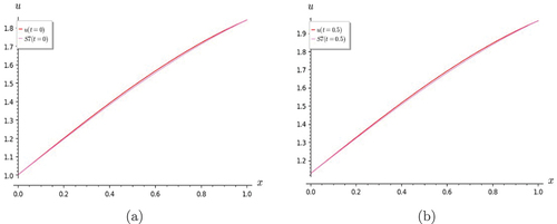
Figure 8. Graphs of Lin and Hom KG equation. (a) S₇ shows good convergence with the exact solution for t = 1.0; (b) the partial sums S₃, S₅ and S₇ are in good agreement for t = 0.

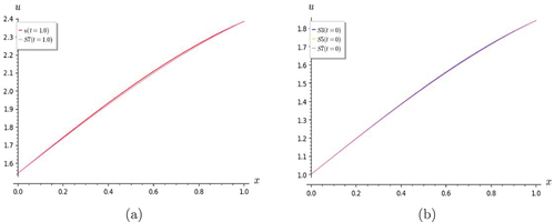
Figure 9. Graphs of Lin and homogeneous KG equation. The partial sums S₃, S₅ and S₇ are in good agreement for (a) t = 0.5 and (b) t = 1.

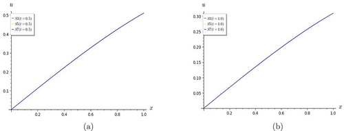
4.4. Linear and non-homogeneous telegraph equation

The method is next applied for solving a non-homogeneous form of the telegraph equation, so that it may be seen how the method works when $\mathit{f}(\mathit{x},\mathit{t})\ne 0$. The equation chosen is (Dehghan & Shokri, 2008)

(16) $\begin{array}{l}{u}_{\mathit{xx}}=u_{\mathit{tt}}+6u_{\mathit{t}}+2\mathit{u}+2e^{-\mathit{t}}\mathit{sin}\mathit{x},0\le \mathit{x}\le 1,\mathit{t}\ge 0.\end{array}$(16)

BCs are taken to be $\mathit{u}(0,\mathit{t})=0$ and $\mathit{u}(1,\mathit{t})=e^{-\mathit{t}}\mathit{sin}1$ from the solution $\mathit{u}(\mathit{x},\mathit{t})=e^{-\mathit{t}}\mathit{sin}\mathit{x}$ (Dehghan & Shokri, 2008). In this equation $\mathit{L}(\mathit{u})=u_{\mathit{xx}}$, $\mathit{R}(\mathit{u})=u_{\mathit{tt}}+6u_{\mathit{t}}+2\mathit{u}$ and $\mathit{f}(\mathit{x},\mathit{t})=2e^{-\mathit{t}}\mathit{sin}\mathit{x}$. The calculations will therefore include $F_k(\mathit{t})$ as well, which makes the whole processes slightly different from the previous cases. S₁ is determined as usual. It is found to be

$\begin{array}{l}{S}_1=(e^{-\mathit{t}}\mathit{sin}1)\mathit{x}.\end{array}$

$\begin{array}{l}{u}_1=c_{0,1}+\mathit{x}{c}_{1,1}+(R_0(S_1)+F_0)\frac{x^2}{2}.\end{array}$

$\begin{array}{l}{R}_0(S_1)={(\frac{{\partial }^2{S}_1}{\mathit{\partial }{t}^2}+6\frac{\partial S_1}{\mathit{\partial t}}+2S_1)}_{\mathit{x}=0}=0,\end{array}$

$\begin{array}{l}{F}_0=\mathit{f}(0,\mathit{t})=0.\end{array}$

Thus

$\begin{array}{l}{u}_1=c_{0,1}+\mathit{x}{c}_{1,1}.\end{array}$

Thereby

$\begin{array}{l}{S}_2=S_1+u_1=(e^{-\mathit{t}}\mathit{sin}1)\mathit{x}+c_{0,1}+\mathit{x}{c}_{1,1}.\end{array}$

Since $c_{0,1}=c_{1,1}=0$, $S_2=S_1$. Proceeding further, set

$\begin{array}{l}{u}_2=c_{0,2}+\mathit{x}{c}_{1,2}+(R_1(S_2)+F_1)\frac{x^3}{6}.\end{array}$

$\begin{array}{ll}{R}_1(S_2)& ={\left(\frac{\mathit{\partial }}{\mathit{\partial x}}\left(\mathit{R}\left(S_2\right)\right)\right)}_{\mathit{x}=0}={\left(\frac{\mathit{\partial }}{\mathit{\partial x}}(\mathit{x}\times -3e^{-\mathit{t}}\mathit{sin}1)\right)}_{\mathit{x}=0}\\ & =-3(\mathit{sin}1)e^{-\mathit{t}}.\end{array}$

$\begin{array}{l}{F}_1={\left(\frac{\mathit{\partial f}}{\mathit{\partial x}}\right)}_{\mathit{x}=0}=2e^{-\mathit{t}}.\end{array}$

$\begin{array}{l}{u}_2=c_{0,2}+\mathit{x}{c}_{1,2}+e^{-\mathit{t}}(2-3\mathit{sin}1)\frac{x^3}{6}.\end{array}$

$\begin{array}{ll}{S}_3& =S_2+u_2=c_{0,2}+\mathit{x}{c}_{1,2}\\ & +e^{-\mathit{t}}(\mathit{xsin}1+(2-3\mathit{sin}1)\frac{x^3}{6})\end{array}$

Setting $S_3(0,\mathit{t})=0$, it is found that $c_{0,2}=0$. Similarly, by setting $S_3(1,\mathit{t})=e^{-\mathit{t}}\mathit{sin}1$,

$\begin{array}{l}{c}_{1,2}=-\frac{(2-3\mathit{sin}1)e^{-\mathit{t}}}{6}.\end{array}$

Figure 10. Graphs of Lin and non-homogeneous telegraph equation. Comparison of S₇ with the exact solution for (a) t = 0 and (b) t = 0.5.

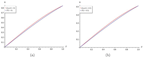
Figure 11. Graphs of Lin and non-homogeneous telegraph equation. S₇ shows good convergence with the exact solution for (a) t = 1.0 and (b) t = 2.0.

Thus

$\begin{array}{l}{S}_3=e^{-\mathit{t}}((\frac{3}{2}\mathit{sin}1-\frac{1}{3})\mathit{x}-(3\mathit{sin}1-2)\frac{x^3}{6}).\end{array}$

The procedures are repeated in a similar way to obtain u₃ = 0, implying that $S_4=S_3$. The next set of operations gives

$\begin{array}{ll}{S}_5& =e^{-\mathit{t}}((\frac{57}{40}\mathit{sin}1-\frac{4}{15})\mathit{x}-(3\mathit{sin}1-2)\frac{x^3}{6}\\ & +(9\mathit{sin}1-8)\frac{x^5}{5!}).\end{array}$

Again, u₅ turns out to be zero, from which S₆ is seen to be equal to S₅. S₇ is determined next as

$\begin{array}{ll}{S}_7& =e^{-\mathit{t}}((\frac{801}{560}\mathit{sin}1-\frac{137}{504})\mathit{x}-(3\mathit{sin}1-2)\frac{x^3}{6}\\ & +(9\mathit{sin}1-8)\frac{x^5}{5!})-e^{-\mathit{t}}\left((27\mathit{sin}1-26)\frac{x^7}{7!}\right).\end{array}$

From the graphs, it is found that the convergence behavior of the truncated series solution S₇ varies from that of the previous examples. The degree of convergence is not very good for low values of t, but it is seen to be improving as t is increased. This is evident when one examines the variation of scale along the vertical axis in Figures 10–12. Figures 12b and 13 show that S₃ is as good an approximation as S₇.

Figure 12. Graphs of Lin and non-homogeneous telegraph equation. S₇ shows good convergence with the exact solution for (a) t = 5.0. (b) The partial sums S₃, S₅ and S₇ converge when t = 0.

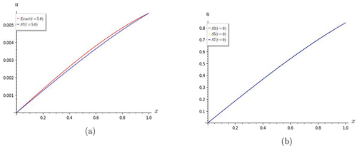
Figure 13. Graphs of Lin and non-homogeneous telegraph equation. The partial sums S₃, S₅ and S₇ converge at $(\mathit{a})\mathit{t}=0.5,(\mathit{b})\mathit{t}=1.0$.

4.5. Linear and non-homogeneous Klein-Gordon equation

An example of the linear and non-homogeneous K-G equation is (Ikram et al., 2021)

(17) $\begin{array}{l}{u}_{\mathit{xx}}=u_{\mathit{tt}}-\mathit{u}+e^{\mathit{x}-\mathit{t}},0\le \mathit{x}\le 1,\mathit{t}\ge 0.\end{array}$(17)

The exact solution of (Equation 17(17) $\begin{array}{l}{u}_{\mathit{xx}}=u_{\mathit{tt}}-\mathit{u}+e^{\mathit{x}-\mathit{t}},0\le \mathit{x}\le 1,\mathit{t}\ge 0.\end{array}$(17) ) is $e^{\mathit{x}-\mathit{t}}$ (Ikram et al., 2021), from which $\mathit{u}(0,\mathit{t})=e^{-\mathit{t}}$ and $\mathit{u}(1,\mathit{t})=e^{1-\mathit{t}}$. $\mathit{L}(\mathit{u})=u_{\mathit{xx}}$, $\mathit{R}(\mathit{u})=(\frac{{\partial }^2}{\mathit{\partial }{t}^2}-1)\mathit{u}$ and $\mathit{f}(\mathit{x},\mathit{t})=e^{\mathit{x}-\mathit{t}}$. The successive partial sums are determined by following the procedures as explained in example 4.4. These are:

$\begin{array}{l}{S}_1=e^{-\mathit{t}}(1+(\mathit{e}-1)\mathit{x});\end{array}$

$\begin{array}{l}{S}_2=e^{-\mathit{t}}(1+(\mathit{e}-\frac{3}{2})\mathit{x}+\frac{x^2}{2});\end{array}$

$\begin{array}{l}{S}_3=e^{-\mathit{t}}(1+(\mathit{e}-1-\frac{1}{2}-\frac{1}{6})\mathit{x}+\frac{x^2}{2}+\frac{x^3}{3!});\end{array}$

$\begin{array}{l}{S}_4=e^{-\mathit{t}}(1+(\mathit{e}-1-\frac{1}{2}-\frac{1}{6}-\frac{1}{24})\mathit{x}+\frac{x^2}{2}+\frac{x^3}{3!}+\frac{x^4}{4!}).\end{array}$

By examining the partial sums obtained so far a clear pattern is seen to be developing in the structure of the solution, from which it may be ascertained that

$\begin{array}{ll}{S}_{\mathrm{\infty }}& =e^{-\mathit{t}}(1+(\mathit{e}-1-\frac{1}{2}-\frac{1}{6}-\frac{1}{24}-\cdots -\frac{1}{\mathit{n}!}-\cdots )\mathit{x})\\ & +e^{-\mathit{t}}(\frac{x^2}{2}+\frac{x^3}{3!}+\frac{x^4}{4!}+\cdots +\frac{x^n}{\mathit{n}!}+\cdots )\\ & =e^{-\mathit{t}}(1+\mathit{x}+\frac{x^2}{2}+\frac{x^3}{3!}+\frac{x^4}{4!}+\cdots +\frac{x^n}{\mathit{n}!}+\cdots )=e^{\mathit{x}-\mathit{t}},\end{array}$

since

$\begin{array}{l}\mathit{e}-1-\frac{1}{2}-\frac{1}{6}-\frac{1}{24}-\cdots -\frac{1}{\mathit{n}!}-\cdots =1.\end{array}$

It is to be noted that $e^{\mathit{x}-\mathit{t}}$ is the closed form solution of (Equation 17(17) $\begin{array}{l}{u}_{\mathit{xx}}=u_{\mathit{tt}}-\mathit{u}+e^{\mathit{x}-\mathit{t}},0\le \mathit{x}\le 1,\mathit{t}\ge 0.\end{array}$(17) ).

4.6. Nonlinear and non-homogeneous telegraph equation

This example is that of a non-linear and non-homogeneous version of the telegraph equation with quadratic non-linearity. The PDE is (Ahmed et al., 2022)

(18) $\begin{array}{l}{u}_{\mathit{xx}}=u_{\mathit{tt}}+2u_{\mathit{t}}+u^2+e^{\mathit{x}-2\mathit{t}}-e^{2\mathit{x}-4\mathit{t}},0\le \mathit{x}\le 1,\mathit{t}\ge 0.\end{array}$(18)

BCs are chosen as $\mathit{u}(0,\mathit{t})=e^{-2\mathit{t}}$ and $\mathit{u}(1,\mathit{t})=e^{1-2\mathit{t}}$ from the closed form solution $\mathit{u}(\mathit{x},\mathit{t})=e^{\mathit{x}-2\mathit{t}}$ (Ahmed et al., 2022). The linear and other operators are

$\begin{array}{ll}& \mathit{L}(\mathit{u})=u_{\mathit{xx}},\mathit{N}(\mathit{u})=u^2,\mathit{R}(\mathit{u})=u_{\mathit{tt}}+2u_{\mathit{t}},\\ & \mathit{f}(\mathit{x},\mathit{t})=e^{\mathit{x}-2\mathit{t}}-e^{2\mathit{x}-4\mathit{t}}.\end{array}$

The additional feature in this case is the presence of the nonlinear term u². Still, u₀, and thereby S₁, can be determined as in the previous examples.

$\begin{array}{l}{S}_1=c_{0,0}+\mathit{x}{c}_{1,0}.\end{array}$

Applying the BCs one obtains $c_{0,0}=e^{-2\mathit{t}}$ and $c_{1,0}=e^{-2\mathit{t}}$$(\mathit{e}-1)$. Thus

$\begin{array}{l}{S}_1=e^{-2\mathit{t}}(1+\mathit{x}(\mathit{e}-1).\end{array}$

$\begin{array}{l}{u}_1=c_{0,1}+\mathit{x}{c}_{1,1}+(R_0(S_1)+N_0(S_1)+F_0)\frac{x^2}{2}.\end{array}$

$\begin{array}{l}{R}_0(S_1)={(\frac{{\partial }^2{S}_1}{\mathit{\partial }{t}^2}+2\frac{\partial S_1}{\mathit{\partial t}})}_{\mathit{x}=0}=0\end{array}$

$\begin{array}{l}{N}_0(S_1)=(S_1^2{)}_{\mathit{x}=0}=e^{-4\mathit{t}};F_0=\mathit{f}(0,\mathit{t})=e^{-2\mathit{t}}-e^{-4\mathit{t}}.\end{array}$

$\begin{array}{l}{u}_1=c_{0,1}+\mathit{x}{c}_{1,1}+e^{-2\mathit{t}}\left(\frac{x^2}{2}\right).\end{array}$

$\begin{array}{l}{S}_2=c_{0,1}+\mathit{x}{c}_{1,1}+e^{-2\mathit{t}}(1+\mathit{x}(\mathit{e}-1)+\frac{x^2}{2}).\end{array}$

The unknowns are determined by applying the BCs to get

$\begin{array}{l}{S}_2=e^{-2\mathit{t}}(1+\mathit{x}(\mathit{e}-\frac{3}{2})+\frac{x^2}{2}).\end{array}$

Procedures are followed to obtain the next two partial sums S₃ and S₄:

$\begin{array}{ll}{S}_3& =((2\mathit{e}-5)e^{-4\mathit{t}}+e^{-2\mathit{t}})\frac{x^3}{6}-e^{-4\mathit{t}}(2\mathit{e}-5+e^{2\mathit{t}})\frac{x}{6}\\ & +e^{-2\mathit{t}}(1+\mathit{x}(\mathit{e}-\frac{3}{2})+\frac{x^2}{2}).\end{array}$

$\begin{array}{ll}{S}_4& =\frac{1}{432}({(3(2\mathit{e}-3)e^{-2\mathit{t}}-(2\mathit{e}-5+e^{2\mathit{t}})e^{-4\mathit{t}})}^2\\ & +18e^{-2\mathit{t}}-36e^{-4\mathit{t}})x^4-\frac{x}{432}((3(2\mathit{e}-3)e^{-2\mathit{t}}\\ & {-(2\mathit{e}-5+{\mathit{e}}^{2\mathit{t}})e^{-4\mathit{t}})}^2+90e^{-2\mathit{t}}+36(4\mathit{e}-11)e^{-4\mathit{t}})\\ & +\frac{1}{6}((2\mathit{e}-5)e^{-4\mathit{t}}+e^{-2\mathit{t}})x^3+e^{-2\mathit{t}}(1+\mathit{x}(\mathit{e}-\frac{3}{2})+\frac{x^2}{2}).\end{array}$

S₄ is taken to represent the solution since it agrees well with it as seen in the graphs in Figures 14 and 15a. S₃ would also be a good approximation since it converges quite well with S₄ (Figures 15b and 16).

Figure 14. Graphs of nonlinear and non-homogeneous telegraph equation. S₄ converges very well with the exact solution when $(\mathit{a})\mathit{t}=0,(\mathit{b})0.5$.

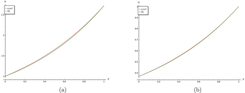
Figure 15. Graphs of nonlinear and non-homogeneous telegraph equation. (a) S₄ converges very well with the exact solution when t = 1.0. (b) shows that partial sums S₃ and S₄ converge when t = 0.

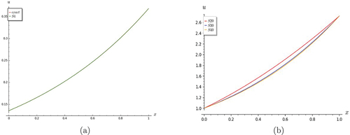
Figure 16. Graphs of nonlinear and non-homogeneous telegraph equation. Partial sums S₃ and S₄ converge when (a) t = 0.5 and (b) 1.0.

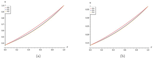
Figure 17. Graphs of Fisher equation. (a) S₃ deviates slightly from the exact solution for t = 0.25.(b) the convergence of S₃ to $\mathit{u}(\mathit{x},\mathit{t})$ is seen to be improving when $\mathit{t}\ge 0.5$, as found in the subsequent graphs for the equation.

4.7. Nonlinear and homogeneous Fishers equation

The Fishers equation models various phenomena in chemical kinetics, autocatalytic chemical reactions, Brownian motion processes, and in the propagation of a mutant gene (Wazwaz, 2008). The nonlinear equation (Loyinmi & Akinfe, 2020) has a term with quadratic non-linearity similar to the one found in the nonlinear telegraph equation solved.

(19) $\begin{array}{l}{u}_{\mathit{xx}}=u_{\mathit{t}}-6\mathit{u}+6u^2.\end{array}$(19)

The BCs

$\begin{array}{l}\mathit{u}(0,\mathit{t})=\frac{1}{{(1+{\mathit{e}}^{-5\mathit{t}})}^2},\mathit{u}(1,\mathit{t})=\frac{1}{{(1+{\mathit{e}}^{1-5\mathit{t}})}^2}.\end{array}$

are taken from the exact solution of the PDE (Loyinmi & Akinfe, 2020)

$\begin{array}{l}\mathit{u}(\mathit{x},\mathit{t})=\frac{1}{{(1+{\mathit{e}}^{\mathit{x}-5\mathit{t}})}^2}.\end{array}$

Following similar procedures applied for solving the nonlinear telegraph equation, the first three partial sums are obtained as

$\begin{array}{l}{S}_1=\frac{1}{{(1+{\mathit{e}}^{-5\mathit{t}})}^2}-\mathit{x}(\frac{1}{{(1+{\mathit{e}}^{-5\mathit{t}})}^2}-\frac{1}{{(1+{\mathit{e}}^{1-5\mathit{t}})}^2}),\end{array}$

$\begin{array}{ll}{S}_2& =\mathit{x}(\frac{2}{{(1+{\mathit{e}}^{-5\mathit{t}})}^2}-\frac{5{\mathit{e}}^{-5\mathit{t}}}{{(1+{\mathit{e}}^{-5\mathit{t}})}^3}-\frac{3}{{(1+{\mathit{e}}^{-5\mathit{t}})}^4}+\frac{1}{{(1+{\mathit{e}}^{1-5\mathit{t}})}^2})\\ & +\frac{1}{{(1+{\mathit{e}}^{-5\mathit{t}})}^2}-x^2(\frac{3}{{(1+{\mathit{e}}^{-5\mathit{t}})}^2}-\frac{5{\mathit{e}}^{-5\mathit{t}}}{{(1+{\mathit{e}}^{-5\mathit{t}})}^3}-\frac{3}{{(1+{\mathit{e}}^{-5\mathit{t}})}^4}),\end{array}$

$\begin{array}{ll}{S}_3& =\frac{1}{{(1+{\mathit{e}}^{-5\mathit{t}})}^2}-\mathit{x}(\frac{2}{{(1+{\mathit{e}}^{-5\mathit{t}})}^2{(1+{\mathit{e}}^{1-5\mathit{t}})}^2}\\ & -\frac{20{\mathit{e}}^{-5\mathit{t}}}{{(1+{\mathit{e}}^{-5\mathit{t}})}^5}-\frac{6}{{(1+{\mathit{e}}^{-5\mathit{t}})}^6})\\ & +\mathit{x}(\frac{4}{{(1+{\mathit{e}}^{-5\mathit{t}})}^2}-\frac{35{\mathit{e}}^{-5\mathit{t}}}{2{(1+{\mathit{e}}^{-5\mathit{t}})}^3}-\frac{5(4-5{\mathit{e}}^{-10\mathit{t}})}{2{(1+{\mathit{e}}^{-5\mathit{t}})}^4}\\ & +\frac{6(1+{\mathit{e}}^{1-5\mathit{t}})-5e^{1-5\mathit{t}}}{3{(1+{\mathit{e}}^{1-5\mathit{t}})}^3})\\ & -x^2(\frac{3}{{(1+{\mathit{e}}^{-5\mathit{t}})}^2}-\frac{5{\mathit{e}}^{-5\mathit{t}}}{{(1+{\mathit{e}}^{-5\mathit{t}})}^3}-\frac{3}{{(1+{\mathit{e}}^{-5\mathit{t}})}^4})\\ & +x^3(\frac{7}{{(1+{\mathit{e}}^{-5\mathit{t}})}^4}+\frac{2}{{(1+{\mathit{e}}^{-5\mathit{t}})}^2{(1+{\mathit{e}}^{1-5\mathit{t}})}^2}\\ & -\frac{20{\mathit{e}}^{-5\mathit{t}}}{{(1+{\mathit{e}}^{-5\mathit{t}})}^5}-\frac{6}{{(1+{\mathit{e}}^{-5\mathit{t}})}^6})\\ & -x^3(\frac{2}{{(1+{\mathit{e}}^{-5\mathit{t}})}^2}-\frac{25{\mathit{e}}^{-5\mathit{t}}}{2{(1+{\mathit{e}}^{-5\mathit{t}})}^3}+\frac{25{\mathit{e}}^{-10\mathit{t}}}{2{(1+{\mathit{e}}^{-5\mathit{t}})}^4}\\ & +\frac{3(1+{\mathit{e}}^{1-5\mathit{t}})-5e^{1-5\mathit{t}}}{3{(1+{\mathit{e}}^{1-5\mathit{t}})}^3})\end{array}$

S₃ is considered a good approximation of $\mathit{u}(\mathit{x},\mathit{t})$ as it is found to converge to the next S₄ quite well (Figure 20). (The expression for S₄ is lengthy and hence is not shown.) Even though S₃ does not agree very well with the exact solution for small values of t, the situation is seen to be improving as t is increased (Figures 17–20).

Figure 18. Graphs of Fisher equation. S₃ converges to $\mathit{u}(\mathit{x},\mathit{t})\mathit{at}(\mathit{a})\mathit{t}=0.75,(\mathit{b})\mathit{t}=1.0$.

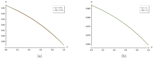
Figure 19. Graphs of Fisher equation. As t gets larger, the convergence of S₃ with $\mathit{u}(\mathit{x},\mathit{t})$ is seen to improve at (a) t=2, and (b) t=5.

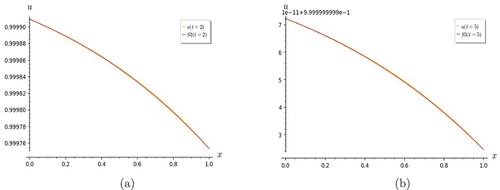
Figure 20. Fishers Eqn.-graphs of Fisher equation showing that S₃ converges to S₄ at (a) t=0.5, and (b) t=1.

4.8. Nonlinear and homogeneous Klein-Gordon equation

The KG equation is considered to be an important PDE of mathematical physics due to its significance in soliton theory and condensed matter physics (Edeki et al., 2019). As mentioned in (Rashidinia et al., 2010) the equation finds applications in solid state physics, nonlinear optics and quantum field theory. A non-linear (and homogeneous) version of the KG equation with cubic non-linearity (Rashidinia et al., 2010)

(20) $\begin{array}{l}{u}_{\mathit{tt}}-\left(\frac{5}{2}\right)u_{\mathit{xx}}+\mathit{u}+\left(\frac{3}{2}\right)u^3=0,\end{array}$(20)

is considered in the interval $0\le \mathit{x}\le 1$, $\mathit{t}\ge 0$. From the exact solution $\mathit{u}(\mathit{x},\mathit{t})=\sqrt{\frac{2}{3}}\mathit{tan}(\frac{\sqrt{2}}{6}(\mathit{t}+2\mathit{x}))$ (Edeki et al., 2019) the following BCs are deduced.

$\begin{array}{l}\mathit{u}(0,\mathit{t})=\sqrt{\frac{2}{3}}\mathit{tan}\left(\frac{\sqrt{2}}{6}\mathit{t}\right),\mathit{u}(1,\mathit{t})=\sqrt{\frac{2}{3}}\mathit{tan}(\frac{\sqrt{2}}{6}(\mathit{t}+2)).\end{array}$

The first three partial sums are determined to be

$\begin{array}{ll}{S}_1& =(\sqrt{\frac{2}{3}}\mathit{tan}(\frac{\sqrt{2}}{6}(\mathit{t}+2))-\sqrt{\frac{2}{3}}\mathit{tan}\left(\frac{\sqrt{2}}{6}\mathit{t}\right))\mathit{x}\\ & +\sqrt{\frac{2}{3}}\mathit{tan}\left(\frac{\sqrt{2}}{6}\mathit{t}\right),\end{array}$

$\begin{array}{ll}{S}_2& =\sqrt{\frac{2}{3}}\mathit{tan}\left(\frac{\sqrt{2}}{6}\mathit{t}\right)\\ & +(\sqrt{\frac{2}{3}}\mathit{tan}(\frac{\sqrt{2}}{6}(\mathit{t}+2))-\sqrt{\frac{2}{3}}\mathit{tan}\left(\frac{\sqrt{2}}{6}\mathit{t}\right))\mathit{x}\\ & +0.\dot{2}\sqrt{\frac{2}{3}}(x^2-\mathit{x})\mathit{sec}{\left(\frac{\sqrt{2}}{6}\mathit{t}\right)}^2\mathit{tan}\left(\frac{\sqrt{2}}{6}\mathit{t}\right),\end{array}$

$\begin{array}{ll}{S}_3& =\sqrt{\frac{2}{3}}\mathit{tan}\left(\frac{\sqrt{2}}{6}\mathit{t}\right)\\ & +\sqrt{\frac{2}{3}}(\mathit{tan}(\frac{\sqrt{2}}{6}(\mathit{t}+2))-\mathit{tan}\left(\frac{\sqrt{2}}{6}\mathit{t}\right))\mathit{x}\\ & +0.\dot{2}\sqrt{\frac{2}{3}}(x^2-\mathit{x}){\sec }^2\left(\frac{\sqrt{2}}{6}\mathit{t}\right)\mathit{tan}\left(\frac{\sqrt{2}}{6}\mathit{t}\right)\\ & -\frac{1}{6}\sqrt{\frac{2}{3}}(x^3-\mathit{x})(0.0\overline{592}{\sec }^2\left(\frac{\sqrt{2}}{6}\mathit{t}\right)+0.113580247)\\ & \times {\sec }^2\left(\frac{\sqrt{2}}{6}\mathit{t}\right)\mathit{tan}\left(\frac{\sqrt{2}}{6}\mathit{t}\right)\\ & -0.2\sqrt{\frac{2}{3}}(x^3-\mathit{x})(0.\dot{2}{\sec }^2\left(\frac{\sqrt{2}\mathit{t}}{6}\right)+1){\tan }^3\left(\frac{\sqrt{2}\mathit{t}}{6}\right)\\ & +0.2\sqrt{\frac{2}{3}}(x^3-\mathit{x})\mathit{tan}(\frac{\sqrt{2}}{6}(\mathit{t}+2)){\tan }^2\left(\frac{\sqrt{2}\mathit{t}}{6}\right)\\ & +\frac{1}{6}\sqrt{\frac{2}{3}}(x^3-\mathit{x})(0.0\dot{4}{\sec }^2\left(\frac{\sqrt{2}}{6}(\mathit{t}+2)\right)+0.4)\\ & \times \mathit{tan}(\frac{\sqrt{2}}{6}(\mathit{t}+2))\\ & -\frac{1}{6}\sqrt{\frac{2}{3}}(x^3-\mathit{x})(0.4\mathit{tan}\left(\frac{\sqrt{2}\mathit{t}}{6}\right))\end{array}$

There is no need to proceed to S₄, since it is seen from the graphs in Figures 21 and 22 that a good rate of convergence is reached.

Figure 21. Graphs of nonlinear KG equation. (a) and (b) S₃ converges to $\mathit{u}(\mathit{x},\mathit{t})$ at (a) t=0 and (b) t=0.5, respectively.

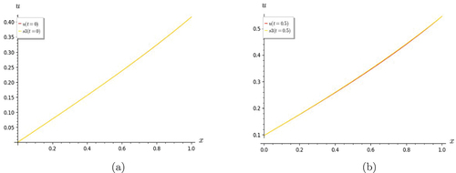
Figure 22. Graphs of nonlinear KG equation. (a) and (b) S₃ converges to $\mathit{u}(\mathit{x},\mathit{t})$ at t=0.75 and t=1.0, respectively.

5. Results and discussion

In this work, a new scheme is devised for solving BVPs of $(1+1)$ second order PDEs with non-homogeneous Dirichlet BCs by combining ModDTM, which is a modification of the DTM in the x-direction, and the ADM. The method has been applied to linear, nonlinear, homogeneous and non-homogeneous versions of the Heat, Telegraph, K-G and Fisher equations to obtain their analytic solutions. Validation of the solutions is done by comparing the graphs of partial sums S_n and the solution functions $\mathit{u}(\mathit{x},\mathit{t})$ plotted using the mathematical software SageMath, in Figures 1 to 22. These figures may be categorised into two types. In the first kind, graphs of the exact solutions are compared with the partial sums; the second kind consists of graphs comparing consecutive partial sums.

For the linear cases, the partial sum-solution is determined up to S₇, though they are found to converge as early as S₅ for the heat equation, and S₃ for the others, excluding the linear and non-homogeneous K-G equation. For the latter, it is found that $S_{\mathrm{\infty }}=\mathit{u}(\mathit{x},\mathit{t})$ is the exact solution. In the case of the linear and non-homogeneous telegraph equation, it is noticed that at t = 0, the $\mathit{max}(|S_7-\mathit{u}(\mathit{x},\mathit{t})|)\approx 0.03$, which occurs in the neighborhood of x = 0.5. This behavior is found to change for the better as t increases. Even though the solution obtained for the Fisher equation exhibits a similar behavior as for the linear, non-homogeneous telegraph equation, it may be said that S₃ is a good approximation of the exact solutions for the nonlinear PDEs. The results discussed here are illustrated in the corresponding graphs found in Figures 1-22. Since the rate of convergence is very good, the graphs, which are multicolored (as indicated in their labels), are seen to be merging with each other.

6. Conclusion

In this paper, a new method termed the NMDT-D is formulated by combining the differential transform from ModDTM and the concept of decomposition of the initial terms from ADM for solving non-homogeneous Dirichlet BVPs of partial differential equations. The method has a straight forward approach, and hence it has simple and uncomplicated procedures that are easily applied. In addition, only a few number of iterations is required to obtain appreciable rates of convergence of the partial sums showing the fast convergence of the method. The graphs show that the solutions obtained are good approximations of the exact ones, as well. Having such a method is significant since there are but a few analytical methods for solving BVPs of PDEs.

For future prospects, it might be examined how the method may be extended for applications to PDEs of higher order, or even of higher dimensions. It may be adapted to suit BVPs of fractional and other types of differential equations as well.

Author details

This work was carried out in collaboration between both the authors as part of a study about various analytic methods for solving partial differential equations in general. It forms part of a project undertaken to find simple procedures for solving different types of boundary value problems in particular.

Disclosure statement

No potential conflict of interest was reported by the author(s).

Funding

The authors declare that funding of any kind was not received for this research or for the publication of this paper.

Data availability statement

No data were used to support the study.

References

- Adomian, G., & Rach, R. (1993). Analytic solution of nonlinear boundary-value problems in several dimensions by decomposition. Journal of Mathematical Analysis and Applications, 174(1), 118–137. https://doi.org/10.1006/jmaa.1993.1105
- Ahmad, J., Bajwa, S., & Siddique, I. (2015). Solving the Klein-Gordan equations via differential transform method. Journal of Science and Arts, 15(1).
- Ahmed, S. A., Qazza, A., & Saadeh, R. (2022). Exact solutions of nonlinear partial differential equations via the new double integral transform combined with iterative method. Axioms, 11(6), 247. https://doi.org/10.3390/axioms11060247
- Al-Ahmad, S., Anakira, N. R., Mamat, M., Jameel, A. F., Alahmad, R., & Alomari, A. K. (2022). Accurate approximate solution of classes of boundary value problems using modified differential transform method. TWMS Journal of Applied and Engineering Mathematics, 12(4), 1228–1238.
- Al-Rozbayani, A. M., & Qasim, A. F. (2023). Modified α-parameterized differential transform method for solving nonlinear generalized gardner equation. Journal of Applied Mathematics, 2023, 1–9. https://doi.org/10.1155/2023/3339655
- Aly, E. H., Ebaid, A., & Rach, R. (2012). Advances in the Adomian decomposition method for solving two-point nonlinear boundary value problems with Neumann boundary conditions. Computers and Mathematics with Applications, 63(6), 1056–1065. https://doi.org/10.1016/j.camwa.2011.12.010
- Chen, C. O. K., & Ho, S. H. (1999). Solving partial differential equations by two-dimensional differential transform method. Applied Mathematics and Computation, 106(2–3), 171–179. https://doi.org/10.1016/S0096-3003(98)10115-7
- Dehghan, M., & Shokri, A. (2008). A numerical method for solving the hyperbolic telegraph equation. Numerical Methods for Partial Differential Equations: An International Journal, 24(4), 1080–1093. https://doi.org/10.1002/num.20306
- Edeki, S. O., Anake, T. A., & Ejoh, S. A. (2019, August). Closed form root of a linear Klein–Gordon equation. Journal of Physics Conference Series, 1299(1), 012138. IOP Publishing: https://doi.org/10.1088/1742-6596/1299/1/012138
- Hussen, S., Uddin, M., & Karim, M. R. (2022). An efficient computational technique for the analysis of telegraph equation. Journal of Engineering Advancements, 3(3), 104–111. https://doi.org/10.38032/jea.2022.03.005
- Ikram, S., Saleem, S., & Hussain, M. Z. (2021). Approximations to linear Klein–gordon equations using Haar wavelet. Ain Shams Engineering Journal, 12(4), 3987–3995. https://doi.org/10.1016/j.asej.2021.01.029
- Jang, B. (2008). Two-point boundary value problems by the extended Adomian decomposition method. Journal of Computational and Applied Mathematics, 219(1), 253–262. https://doi.org/10.1016/j.cam.2007.07.036
- Kharrat, B. N., & Toma, G. (2020). Differential transform method for solving boundary value problems represented by system of ordinary differential equations of 4 order. World Applied Sciences Journal, 38(1), 25–31.
- Kreyszig, E. (1991). Introductory functional analysis with applications (Vol. 17). John Wiley and Sons.
- Lesnic, D., & Elliott, L. (1999). The decomposition approach to inverse heat conduction. Journal of Mathematical Analysis and Applications, 232(1), 82–98. https://doi.org/10.1006/jmaa.1998.6243
- Lock, C. G. J., Greeff, J., & Joubert, S. (2007). Modelling of Telegraph Equations in Transmission Lines [ Doctoral dissertation], Tshwane University of Technology.
- Loyinmi, A. C., & Akinfe, T. K. (2020). Exact solutions to the family of fisher’s reaction-diffusion equation using Elzaki homotopy transformation perturbation method. Engineering Reports, 2(2), e12084. https://doi.org/10.1002/eng2.12084
- Lu, J. (2007). Variational iteration method for solving two-point boundary value problems. Journal of Computational and Applied Mathematics, 207(1), 92–95. https://doi.org/10.1016/j.cam.2006.07.014
- Mukhtarov, O., Yücel, M., & Aydemir, K. (2021). A new generalization of the differential transform method for solving boundary value problems. Journal of New Results in Science, 10(2), 49–58.
- Nayar, H., & Phiri, P. A. (2020). A new modification of the differential transform method. Asian Journal of Mathematics and Computer Research, 27(3), 38–51.
- Nemrat, A. A., Hailat, I., & Zainuddin, Z. (2019, November). Approximate solutions of some linear boundary value problems using the homotopy analysis method combined with sumudu transform. Journal of Physics Conference Series, 1366(1), 012038. IOP Publishing: https://doi.org/10.1088/1742-6596/1366/1/012038
- Nemrat, A. A., & Zainuddin, Z. (2020). Sumudu transform and variational iteration method to solve two point second order linear boundary value problems. ASM Sciences Journal, 13. https://doi.org/10.32802/asmscj.2020.sm26(4.22)
- Rashidinia, J., Ghasemi, M., & Jalilian, R. (2010). Numerical solution of the nonlinear Klein–Gordon equation. Journal of Computational and Applied Mathematics, 233(8), 1866–1878. https://doi.org/10.1016/j.cam.2009.09.023
- Soltanalizadeh, B. (2011). Differential transformation method for solving one-space-dimensional telegraph equation. Computational and Applied Mathematics, 30(3), 639–653. https://doi.org/10.1590/S1807-03022011000300009
- Wazwaz, A. M. (2008). Analytic study on burgers, Fisher, huxley equations and combined forms of these equations. Applied Mathematics and Computation, 195(2), 754–761. https://doi.org/10.1016/j.amc.2007.05.020
- Yun, Y. S., Wen, Y., Chaolu, T., & Rach, R. (2019). A segmented Adomian algorithm for the boundary value problem of a second-order partial differential equation on a plane triangle area. Advances in Difference Equations, 2019(1), 1–13. https://doi.org/10.1186/s13662-019-2329-4