An accelerated numerical computation for singularly perturbed Robin-type parabolic problems with small parameters

ABSTRACT

This study presents a computational method for solving singularly perturbed Robin-type parabolic problem with two perturbation parameters. The fitted operator method in the space direction and the implicit Euler approach in the time direction are used to discretize the problem on a uniform mesh. Furthermore, the new fitted operator method is used to discretize the Robin boundary conditions. The linear order of parameter-uniform convergence has been investigated in both the time and space variables. The application of the Richardson extrapolation approach enhanced the accuracy and rate of convergence of the present method from linear to quadratic order. On the computations of two numerical examples, the theoretical and computational results agreed upon.

KEYWORDS:

• An accelerated numerical computation
• Robin-type problem
• two parameters
• Richardson extrapolation

1. Introduction

Differential equations, which consider small positive parameters, are often used to describe real-world engineering and applied mathematics problems. Many scientists, researchers, and engineers investigated differential equations with a single parameter $\mathit{\epsilon }(0<\mathit{\epsilon }\ll 1)$ multiplied to the highest derivative in the equation. This type of equation is a singularly perturbed differential equation with one-parameter. Several studies published in the literature explore asymptotic, analytical, and numerical solutions to ordinary and partial differential equations with one-parameter. Asymptotic and numerical solutions to two-parameter singularly perturbed differential equations have received relatively little study in comparison to their one-parameter counterparts. It is generally understood that the existence of small parameters in differential equations creates boundary and/or interior layers to appear in the solution. O’Malley (1967a, 1967b, 1969) and Chen and O’Malley (1974) proposed singularly perturbed problems with two small parameters and investigated their asymptotic solutions.

Various numerical approaches were developed subsequently that improved the accuracy of the asymptotic approaches proposed by O’Malley and his co-workers. Patidar (2008) was the first scholar to design a robust fitted operator finite difference approach for a two-parameter singular perturbation ordinary differential equations. The numerical solution of two-parametric singularly perturbed parabolic partial differential equations with non-smooth data was studied in Chandru et al (2018, 2019). Various researchers proposed parameter-uniform numerical methods for solving two-parameter singularly perturbed parabolic problems, see in O’Riordan et al. (2006), Kadalbajoo and Yadaw (2012), Das and Mehrmann (2016), Jha and Kadalbajoo (2015), Munyakazi (2015), Gupta et al. (2019), Mekonnen et al (2020, 2021). Bullo et al (2021b, 2021b, 2022) and Sumit et al. (2020). All of the preceding works dealt with singularly perturbed two-parameter parabolic problems with initial and Dirichlet boundary conditions. Some parameter-robust numerical methods are developed by Hailu et al (2022b, 2022a), Daba et al. (2022), Hassen et al. (2023) and Duressa et al. (2023) to solve different kinds of singularly perturbed problems. However, different numerical treatments have been reported for one-parameter singularly perturbed problems of convection-diffusion and reaction-diffusion types with initial and Robin boundary conditions in Hemker et al. (2002), Das and Natesan (2013a), Selvi and Ramanujam (2017), Mbroh et al. (2020), Janani Jayalakshmi and Tamilselvan (2020), Das et al. (2020), Sunil et al. (2021), Gelu et al (2021, 2022a, 2022b, 2022, 2023b, 2023a), Saini et al (2023, 2024) and Srivastava et al. (2023), S. Kumar et al. (2023).

The Haar wavelet method for space direction on a Shishkin mesh and the implicit Euler method for time direction on a uniform mesh are used to solve the problem under consideration by D. Kumar and Deswal (2022). They determined the maximum residual errors since the double mesh approach cannot be used to solve all kinds of problems approximated using the Haar wavelet scheme. Despite the fact that they claimed their method is robust, no one can observe a stable and parameter-uniform convergence from their numerical output. Motivated by this work, we construct an efficient, stable and parameter-uniform numerical method that is based on a uniform mesh and combines the fitted operator finite difference method in space direction with implicit Euler method in time direction. The proposed method leads to the linear order of convergence in time and space directions. The use of Richardson extrapolation improved the accuracy by increasing the order of convergence from linear to quadratic. Two test examples are used to verify the appilcability of the present method. The results we obtain indicate that the method provides stable and parameter-uniform convergence irrespective of ɛ and µ. The problem considered is the following two-parameter singularly perturbed parabolic problem

(1) $\begin{array}{ll}{\mathcal{L}}_{\mathit{\epsilon },\mathit{\mu }}\mathit{w}(\mathit{x},\mathit{t})& \equiv \frac{\mathit{\partial w}}{\mathit{\partial t}}-\mathit{\epsilon }\frac{{\mathit{\partial }}^2\mathit{w}}{\mathit{\partial }{x}^2}-\mathit{\mu a}(\mathit{x},\mathit{t})\frac{\mathit{\partial w}}{\mathit{\partial x}}+\mathit{b}(\mathit{x},\mathit{t})\mathit{w}(\mathit{x},\mathit{t})\\ =\mathit{g}(\mathit{x},\mathit{t}),(\mathit{x},\mathit{t})\in \mathrm{\Omega },\end{array}$(1)

along with the initial condition and Robin boundary conditions

(2) $\{\begin{array}{ll}\mathit{w}(\mathit{x},0)=\mathit{\phi }(\mathit{x}),& 0\le \mathit{x}\le 1,\\ B_{\mathit{l},\mathit{\epsilon }}\mathit{w}(0,\mathit{t})\equiv {\beta }_1(0,\mathit{t})\mathit{w}(0,\mathit{t})-\mathit{\epsilon }{\beta }_2(0,\mathit{t})\frac{\mathit{\partial w}(0,\mathit{t})}{\mathit{\partial x}}=\mathit{\eta }(\mathit{t}),& 0<\mathit{t}\le \mathit{T},\\ B_{\mathit{r},\mathit{\epsilon }}\mathit{w}(1,\mathit{t})\equiv {\lambda }_1(1,\mathit{t})\mathit{w}(1,\mathit{t})+\mathit{\epsilon }{\lambda }_2(1,\mathit{t})\frac{\mathit{\partial w}(1,\mathit{t})}{\mathit{\partial x}}=\mathit{\theta }(\mathit{t}),& 0<\mathit{t}\le \mathit{T},\end{array}$(2)

where $\mathit{\epsilon }(0<\mathit{\epsilon }\ll 1)$ and $\mathit{\mu }(0\le \mathit{\mu }\ll 1)$ are the small perturbation parameters and $\mathrm{\Omega }=(0,1)\times (0,\mathit{T}]$. The functions $\mathit{a}(\mathit{x},\mathit{t}),\mathit{b}(\mathit{x},\mathit{t}),\mathit{g}(\mathit{x},\mathit{t})$ in $\overline{\mathrm{\Omega }}$; ${\beta }_1(0,\mathit{t}),{\beta }_2(0,\mathit{t}),\text{allowbreak}{\lambda }_1(1,\mathit{t}),{\lambda }_2(1,\mathit{t}),\mathit{\eta }(\mathit{t}),\mathit{\theta }(\mathit{t})$ for $0<\mathit{t}\le \mathit{T}$ and $\mathit{\phi }(\mathit{x})\text{for}0\le \mathit{x}\le 1$ are assumed to be smooth and bounded such that $\mathit{a}(\mathit{x},\mathit{t})\ge \mathit{\alpha }>0,\mathit{b}(\mathit{x},\mathit{t})\ge \mathit{\zeta }>0,\mathrm{\forall }(\mathit{x},\mathit{t})\in \overline{\mathrm{\Omega }}.$ Moreover, we assume that the constants ${\beta }_1,{\beta }_2,{\lambda }_1,{\lambda }_2$ given in Robin boundary conditions satisfy the conditions (Mbroh et al., 2020)

$\begin{array}{l}{\beta }_1(0,\mathit{t}),{\beta }_2(0,\mathit{t})>0,{\beta }_1(0,\mathit{t})+{\beta }_2(0,\mathit{t})>0,\\ {\lambda }_1(1,\mathit{t}),{\lambda }_2(1,\mathit{t})\ge 0,{\lambda }_1(1,\mathit{t})+{\lambda }_2(1,\mathit{t})>0.\end{array}$

Furthermore, we define $\mathit{\gamma }=\underset{(x,t)\in \overline{\mathrm{\Omega }}}{max}\frac{\mathit{b}(\mathit{x},\mathit{t})}{\mathit{a}(\mathit{x},\mathit{t})}.$ If µ = 0, then (1(1) $\begin{array}{ll}{\mathcal{L}}_{\mathit{\epsilon },\mathit{\mu }}\mathit{w}(\mathit{x},\mathit{t})& \equiv \frac{\mathit{\partial w}}{\mathit{\partial t}}-\mathit{\epsilon }\frac{{\mathit{\partial }}^2\mathit{w}}{\mathit{\partial }{x}^2}-\mathit{\mu a}(\mathit{x},\mathit{t})\frac{\mathit{\partial w}}{\mathit{\partial x}}+\mathit{b}(\mathit{x},\mathit{t})\mathit{w}(\mathit{x},\mathit{t})\\ =\mathit{g}(\mathit{x},\mathit{t}),(\mathit{x},\mathit{t})\in \mathrm{\Omega },\end{array}$(1) ) is called a singularly perturbed parabolic reaction-diffusion problem which exhibits boundary layers of width $\mathit{O}(\sqrt{\mathit{\epsilon }})$ at x = 0 and x = 1. If µ = 1, then (1(1) $\begin{array}{ll}{\mathcal{L}}_{\mathit{\epsilon },\mathit{\mu }}\mathit{w}(\mathit{x},\mathit{t})& \equiv \frac{\mathit{\partial w}}{\mathit{\partial t}}-\mathit{\epsilon }\frac{{\mathit{\partial }}^2\mathit{w}}{\mathit{\partial }{x}^2}-\mathit{\mu a}(\mathit{x},\mathit{t})\frac{\mathit{\partial w}}{\mathit{\partial x}}+\mathit{b}(\mathit{x},\mathit{t})\mathit{w}(\mathit{x},\mathit{t})\\ =\mathit{g}(\mathit{x},\mathit{t}),(\mathit{x},\mathit{t})\in \mathrm{\Omega },\end{array}$(1) ) is well-known singularly perturbed parabolic convection-diffusion-reaction problem showing parabolic boundary layer of width $\mathit{O}(\mathit{\epsilon })$ appear near x = 0 (O’Riordan et al., 2006). Depending on the order of the parameters, two possibilities arise. Firstly, when we assume $\frac{\epsilon }{{\mu }^2}\to 0$ as $\mathit{\mu }\to 0$, a layer of width $\mathit{O}(\frac{\epsilon }{\mu })$ and $\mathit{O}(\mathit{\mu })$ appear in the vicinity of x = 0 and x = 1, respectively. Secondly, when we suppose $\frac{{\mu }^2}{\mathit{\epsilon }}\to 0$ as $\mathit{\epsilon }\to 0$, boundary layers of width $\mathit{O}(\sqrt{\mathit{\epsilon }})$ appear in the vicinity of the boundary x = 0 and x = 1.

The existence and uniqueness for the solution to Eq. (1)(1) $\begin{array}{ll}{\mathcal{L}}_{\mathit{\epsilon },\mathit{\mu }}\mathit{w}(\mathit{x},\mathit{t})& \equiv \frac{\mathit{\partial w}}{\mathit{\partial t}}-\mathit{\epsilon }\frac{{\mathit{\partial }}^2\mathit{w}}{\mathit{\partial }{x}^2}-\mathit{\mu a}(\mathit{x},\mathit{t})\frac{\mathit{\partial w}}{\mathit{\partial x}}+\mathit{b}(\mathit{x},\mathit{t})\mathit{w}(\mathit{x},\mathit{t})\\ =\mathit{g}(\mathit{x},\mathit{t}),(\mathit{x},\mathit{t})\in \mathrm{\Omega },\end{array}$(1) -(2(2) $\{\begin{array}{ll}\mathit{w}(\mathit{x},0)=\mathit{\phi }(\mathit{x}),& 0\le \mathit{x}\le 1,\\ B_{\mathit{l},\mathit{\epsilon }}\mathit{w}(0,\mathit{t})\equiv {\beta }_1(0,\mathit{t})\mathit{w}(0,\mathit{t})-\mathit{\epsilon }{\beta }_2(0,\mathit{t})\frac{\mathit{\partial w}(0,\mathit{t})}{\mathit{\partial x}}=\mathit{\eta }(\mathit{t}),& 0<\mathit{t}\le \mathit{T},\\ B_{\mathit{r},\mathit{\epsilon }}\mathit{w}(1,\mathit{t})\equiv {\lambda }_1(1,\mathit{t})\mathit{w}(1,\mathit{t})+\mathit{\epsilon }{\lambda }_2(1,\mathit{t})\frac{\mathit{\partial w}(1,\mathit{t})}{\mathit{\partial x}}=\mathit{\theta }(\mathit{t}),& 0<\mathit{t}\le \mathit{T},\end{array}$(2) ) can be established under the assumption that the data are H$\ddot{o}$lder continuous and satisfy an appropriate compatibility conditions at the corner points (0, 0) and (1, 0). The boundary functions $\mathit{\eta }(\mathit{t}),\mathit{\theta }(\mathit{t})\in C^{\mathit{k}}([0,\mathit{T}]),\mathit{\phi }(\mathit{x})\in C^{(1,\mathit{k})}([0,1])$ should satisfy the k^th order compatibility condition for the initial function if

$\begin{array}{l}\frac{{\partial }^{\mathit{k}}}{\mathit{\partial }{t}^{\mathit{k}}}({\beta }_1(0,0)\mathit{\phi }(0)-\mathit{\epsilon }{\beta }_2(0,0)\frac{\mathit{\partial \phi }(0)}{\mathit{\partial x}})=\frac{{\mathit{d}}^{\mathit{k}}\mathit{\eta }(0)}{\mathit{\partial }{t}^{\mathit{k}}},\\ \frac{{\partial }^{\mathit{k}}}{\mathit{\partial }{t}^{\mathit{k}}}({\lambda }_1(1,0)\mathit{\phi }(1)+\mathit{\epsilon }{\lambda }_2(1,0)\frac{\mathit{\partial \phi }(1)}{\mathit{\partial x}})=\frac{{\mathit{d}}^{\mathit{k}}\mathit{\theta }(0)}{\mathit{\partial }{t}^{\mathit{k}}},\\ \frac{\mathit{\partial \eta }(0)}{\mathit{\partial t}}-\mathit{\epsilon }\frac{{\mathit{\partial }}^2\mathit{\phi }(0)}{\mathit{\partial }{x}^2}-\mathit{\mu a}(0,0)\frac{\mathit{\partial \phi }(0)}{\mathit{\partial x}}+\mathit{b}(0,0)\mathit{\phi }(0)=\mathit{g}(0,0),\\ \frac{\mathit{\partial \theta }(1)}{\mathit{\partial t}}-\mathit{\epsilon }\frac{{\mathit{\partial }}^2\mathit{\phi }(1)}{\mathit{\partial }{x}^2}-\mathit{\mu a}(1,0)\frac{\mathit{\partial \phi }(1)}{\mathit{\partial x}}+\mathit{b}(1,0)\mathit{\phi }(1)=\mathit{g}(1,0).\end{array}$

Now, we introduce the regularity of the solutions to the time-dependent problems in some spaces. To guarantee the existence of the unique solution of problem (1(1) $\begin{array}{ll}{\mathcal{L}}_{\mathit{\epsilon },\mathit{\mu }}\mathit{w}(\mathit{x},\mathit{t})& \equiv \frac{\mathit{\partial w}}{\mathit{\partial t}}-\mathit{\epsilon }\frac{{\mathit{\partial }}^2\mathit{w}}{\mathit{\partial }{x}^2}-\mathit{\mu a}(\mathit{x},\mathit{t})\frac{\mathit{\partial w}}{\mathit{\partial x}}+\mathit{b}(\mathit{x},\mathit{t})\mathit{w}(\mathit{x},\mathit{t})\\ =\mathit{g}(\mathit{x},\mathit{t}),(\mathit{x},\mathit{t})\in \mathrm{\Omega },\end{array}$(1) )-(2(2) $\{\begin{array}{ll}\mathit{w}(\mathit{x},0)=\mathit{\phi }(\mathit{x}),& 0\le \mathit{x}\le 1,\\ B_{\mathit{l},\mathit{\epsilon }}\mathit{w}(0,\mathit{t})\equiv {\beta }_1(0,\mathit{t})\mathit{w}(0,\mathit{t})-\mathit{\epsilon }{\beta }_2(0,\mathit{t})\frac{\mathit{\partial w}(0,\mathit{t})}{\mathit{\partial x}}=\mathit{\eta }(\mathit{t}),& 0<\mathit{t}\le \mathit{T},\\ B_{\mathit{r},\mathit{\epsilon }}\mathit{w}(1,\mathit{t})\equiv {\lambda }_1(1,\mathit{t})\mathit{w}(1,\mathit{t})+\mathit{\epsilon }{\lambda }_2(1,\mathit{t})\frac{\mathit{\partial w}(1,\mathit{t})}{\mathit{\partial x}}=\mathit{\theta }(\mathit{t}),& 0<\mathit{t}\le \mathit{T},\end{array}$(2) ), we need to assume that the coefficients of the considered problem are H$\ddot{o}$lder continuous in both x and t with exponent λ, where $\mathit{\lambda }\in (0,1)$. A function $\mathit{u}(\mathit{x},\mathit{t})$ is said to be H$\ddot{o}$lder continuous with respect to exponent λ if,

$\begin{array}{l}|\mathit{u}(\mathit{x},\mathit{t})-\mathit{u}(x^{\prime },t^{\prime })|\le \mathit{C}(|\mathit{x}-x^{\prime }{|}^2+|\mathit{t}-t^{\prime }|{)}^{\mathit{\lambda }/2}.\end{array}$

for all $(x^{\prime },t^{\prime })\in \mathrm{\Omega }$. Assume that the coefficient of the parabolic PDE and the initial boundary condition in (1(1) $\begin{array}{ll}{\mathcal{L}}_{\mathit{\epsilon },\mathit{\mu }}\mathit{w}(\mathit{x},\mathit{t})& \equiv \frac{\mathit{\partial w}}{\mathit{\partial t}}-\mathit{\epsilon }\frac{{\mathit{\partial }}^2\mathit{w}}{\mathit{\partial }{x}^2}-\mathit{\mu a}(\mathit{x},\mathit{t})\frac{\mathit{\partial w}}{\mathit{\partial x}}+\mathit{b}(\mathit{x},\mathit{t})\mathit{w}(\mathit{x},\mathit{t})\\ =\mathit{g}(\mathit{x},\mathit{t}),(\mathit{x},\mathit{t})\in \mathrm{\Omega },\end{array}$(1) )–(2(2) $\{\begin{array}{ll}\mathit{w}(\mathit{x},0)=\mathit{\phi }(\mathit{x}),& 0\le \mathit{x}\le 1,\\ B_{\mathit{l},\mathit{\epsilon }}\mathit{w}(0,\mathit{t})\equiv {\beta }_1(0,\mathit{t})\mathit{w}(0,\mathit{t})-\mathit{\epsilon }{\beta }_2(0,\mathit{t})\frac{\mathit{\partial w}(0,\mathit{t})}{\mathit{\partial x}}=\mathit{\eta }(\mathit{t}),& 0<\mathit{t}\le \mathit{T},\\ B_{\mathit{r},\mathit{\epsilon }}\mathit{w}(1,\mathit{t})\equiv {\lambda }_1(1,\mathit{t})\mathit{w}(1,\mathit{t})+\mathit{\epsilon }{\lambda }_2(1,\mathit{t})\frac{\mathit{\partial w}(1,\mathit{t})}{\mathit{\partial x}}=\mathit{\theta }(\mathit{t}),& 0<\mathit{t}\le \mathit{T},\end{array}$(2) ) are sufficiently smooth, and satisfy the necessary compatibility conditions. Then, the problems (1(1) $\begin{array}{ll}{\mathcal{L}}_{\mathit{\epsilon },\mathit{\mu }}\mathit{w}(\mathit{x},\mathit{t})& \equiv \frac{\mathit{\partial w}}{\mathit{\partial t}}-\mathit{\epsilon }\frac{{\mathit{\partial }}^2\mathit{w}}{\mathit{\partial }{x}^2}-\mathit{\mu a}(\mathit{x},\mathit{t})\frac{\mathit{\partial w}}{\mathit{\partial x}}+\mathit{b}(\mathit{x},\mathit{t})\mathit{w}(\mathit{x},\mathit{t})\\ =\mathit{g}(\mathit{x},\mathit{t}),(\mathit{x},\mathit{t})\in \mathrm{\Omega },\end{array}$(1) )–(2(2) $\{\begin{array}{ll}\mathit{w}(\mathit{x},0)=\mathit{\phi }(\mathit{x}),& 0\le \mathit{x}\le 1,\\ B_{\mathit{l},\mathit{\epsilon }}\mathit{w}(0,\mathit{t})\equiv {\beta }_1(0,\mathit{t})\mathit{w}(0,\mathit{t})-\mathit{\epsilon }{\beta }_2(0,\mathit{t})\frac{\mathit{\partial w}(0,\mathit{t})}{\mathit{\partial x}}=\mathit{\eta }(\mathit{t}),& 0<\mathit{t}\le \mathit{T},\\ B_{\mathit{r},\mathit{\epsilon }}\mathit{w}(1,\mathit{t})\equiv {\lambda }_1(1,\mathit{t})\mathit{w}(1,\mathit{t})+\mathit{\epsilon }{\lambda }_2(1,\mathit{t})\frac{\mathit{\partial w}(1,\mathit{t})}{\mathit{\partial x}}=\mathit{\theta }(\mathit{t}),& 0<\mathit{t}\le \mathit{T},\end{array}$(2) ) have unique solution $\mathit{u}(\mathit{x},\mathit{t})\in C_{\lambda }^4(\overline{\mathrm{\Omega }}),$ where the space of all functions having H$\ddot{o}$lder continuous derivatives is defined as

$\begin{array}{l}{C}_{\lambda }^4(\mathrm{\Omega })=min\{\mathit{u}:{\displaystyle \frac{{\mathit{\partial }}^{\mathit{i}+\mathit{j}}\mathit{u}}{\mathit{\partial }{x}^{\mathit{i}}\mathit{\partial }{t}^{\mathit{j}}}}\in C_{\lambda }^0(\mathrm{\Omega })\}\end{array}$

for all non negative integers $\mathit{i},\mathit{j}$ with $0\le \mathit{i}+2\mathit{j}\le 4$ and here $C_{\lambda }^0(\mathrm{\Omega })$ is the set of H$\ddot{o}$lder continuous functions with exponent λ.

The mathematical models related to two-parameter singularly perturbed problem of type (1(1) $\begin{array}{ll}{\mathcal{L}}_{\mathit{\epsilon },\mathit{\mu }}\mathit{w}(\mathit{x},\mathit{t})& \equiv \frac{\mathit{\partial w}}{\mathit{\partial t}}-\mathit{\epsilon }\frac{{\mathit{\partial }}^2\mathit{w}}{\mathit{\partial }{x}^2}-\mathit{\mu a}(\mathit{x},\mathit{t})\frac{\mathit{\partial w}}{\mathit{\partial x}}+\mathit{b}(\mathit{x},\mathit{t})\mathit{w}(\mathit{x},\mathit{t})\\ =\mathit{g}(\mathit{x},\mathit{t}),(\mathit{x},\mathit{t})\in \mathrm{\Omega },\end{array}$(1) ) arise in transport phenomena in chemistry, biology, chemical reactor theory (Vasil’eva, 1963), lubrication theory (DiPrima, 1968) and dc motor theory (Bigge & Bohl, 1985) and flow through unsaturated porous media (Bhathawala & Verma, 1975). In two-parameter singular perturbation problems, the diffusion and convection terms are multiplied by the perturbation parameters.

This article is divided as follows. Section 2 outlines the analytical properties of the continuous problem. Section 3 discuss about fully discrete numerical scheme. Section 4 demonstrates the stability and convergence analysis of a fully discretized problem. Section 4 gives the numerical results and discussions. The paper ends with conclusion in Section 6.

2. Analytical properties

In this section, we put a priori bounds for the solution and its corresponding derivatives. The assumptions given for (1(1) $\begin{array}{ll}{\mathcal{L}}_{\mathit{\epsilon },\mathit{\mu }}\mathit{w}(\mathit{x},\mathit{t})& \equiv \frac{\mathit{\partial w}}{\mathit{\partial t}}-\mathit{\epsilon }\frac{{\mathit{\partial }}^2\mathit{w}}{\mathit{\partial }{x}^2}-\mathit{\mu a}(\mathit{x},\mathit{t})\frac{\mathit{\partial w}}{\mathit{\partial x}}+\mathit{b}(\mathit{x},\mathit{t})\mathit{w}(\mathit{x},\mathit{t})\\ =\mathit{g}(\mathit{x},\mathit{t}),(\mathit{x},\mathit{t})\in \mathrm{\Omega },\end{array}$(1) ) and (2(2) $\{\begin{array}{ll}\mathit{w}(\mathit{x},0)=\mathit{\phi }(\mathit{x}),& 0\le \mathit{x}\le 1,\\ B_{\mathit{l},\mathit{\epsilon }}\mathit{w}(0,\mathit{t})\equiv {\beta }_1(0,\mathit{t})\mathit{w}(0,\mathit{t})-\mathit{\epsilon }{\beta }_2(0,\mathit{t})\frac{\mathit{\partial w}(0,\mathit{t})}{\mathit{\partial x}}=\mathit{\eta }(\mathit{t}),& 0<\mathit{t}\le \mathit{T},\\ B_{\mathit{r},\mathit{\epsilon }}\mathit{w}(1,\mathit{t})\equiv {\lambda }_1(1,\mathit{t})\mathit{w}(1,\mathit{t})+\mathit{\epsilon }{\lambda }_2(1,\mathit{t})\frac{\mathit{\partial w}(1,\mathit{t})}{\mathit{\partial x}}=\mathit{\theta }(\mathit{t}),& 0<\mathit{t}\le \mathit{T},\end{array}$(2) ) ensure that the differential operator ${\mathcal{L}}_{\mathit{\epsilon },\mathit{\mu }}$ satisfies the following maximum principle.

Lemma 2.1.

Assume that $\mathrm{\Phi }(\mathit{x},\mathit{t})$ be smooth function satisfying $\mathrm{\Phi }(\mathit{x},0)\ge 0$ on $\mathit{x}\in (0,1)$, $B_{\mathit{l},\mathit{\epsilon }}\mathrm{\Phi }(0,\mathit{t})\ge 0$, $B_{\mathit{r},\mathit{\epsilon }}\mathrm{\Phi }(1,\mathit{t})\ge 0$ on $\mathit{t}\in (0,\mathit{T}]$. If ${\mathcal{L}}_{\mathit{\epsilon },\mathit{\mu }}\mathrm{\Phi }(\mathit{x},\mathit{t})\ge 0,(\mathit{x},\mathit{t})\in \mathrm{\Omega }$, then $\mathrm{\Phi }(\mathit{x},\mathit{t})\ge 0$, $(\mathit{x},\mathit{t})\in \overline{\mathrm{\Omega }}$.

Proof.

Let an arbitrary smooth function Φ takes its minimum value at the point $(\mathit{\xi },\mathit{\varsigma })\in \overline{\mathrm{\Omega }}$ such that $\mathrm{\Phi }(\mathit{\xi },\mathit{\varsigma })=\underset{(x,t)\in \overline{\mathrm{\Omega }}}{min}\mathrm{\Phi }(\mathit{x},\mathit{t})$ and assume that $\mathrm{\Phi }(\mathit{\xi },\mathit{\varsigma })<0$. This implies that $(\mathit{\xi },\mathit{\varsigma })$ is not on the boundary.

Case (i): For $(\mathit{\xi },\mathit{\varsigma })\in \{0\}\times (0,\mathit{T}]$, we have $\frac{\mathit{\partial }\mathrm{\Phi }}{\mathit{\partial x}}(0,\mathit{\varsigma })\ge 0$. Hence, $B_{\mathit{l},\mathit{\epsilon }}\mathrm{\Phi }(0,\mathit{\varsigma })={\beta }_1(0,\mathit{t})\mathrm{\Phi }(0,\mathit{\varsigma })-\mathit{\epsilon }{\beta }_2(0,\mathit{t})\frac{\mathit{\partial }\mathrm{\Phi }}{\mathit{\partial x}}(0,\mathit{\varsigma })<0$, which contradicts the assumption.

Case (ii): For $(\mathit{\xi },\mathit{\varsigma })\in \{1\}\times (0,\mathit{T}]$, we have $\frac{\mathit{\partial }\mathrm{\Phi }}{\mathit{\partial x}}(0,\mathit{\eta })\le 0$. Hence, $B_{\mathit{r},\mathit{\epsilon }}\mathrm{\Phi }(1,\mathit{\varsigma })={\lambda }_1(1,\mathit{t})\mathrm{\Phi }(1,\mathit{\varsigma })+{\lambda }_2(1,\mathit{t})\frac{\mathit{\partial }\mathrm{\Phi }}{\mathit{\partial x}}(1,\mathit{\varsigma })<0$, which contradicts the assumption.

Case (iii): For $(\mathit{\xi },\mathit{\varsigma })\in \mathrm{\Omega }$, as it attains minimum at $(\mathit{\xi },\mathit{\varsigma })$, we have $\frac{\mathit{\partial }\mathrm{\Phi }}{\mathit{\partial t}}(\mathit{\xi },\mathit{\varsigma })=0$, $\frac{\mathit{\partial }\mathrm{\Phi }}{\mathit{\partial x}}(\mathit{\xi },\mathit{\varsigma })=0$ and $\frac{{\partial }^2\mathrm{\Phi }}{\mathit{\partial }{x}^2}(\mathit{\xi },\mathit{\varsigma })\ge 0$. Hence,

$\begin{array}{ll}{\mathcal{L}}_{\mathit{\epsilon },\mathit{\mu }}\mathrm{\Phi }(\mathit{\xi },\mathit{\varsigma })& =\frac{\mathit{\partial }\mathrm{\Phi }}{\mathit{\partial t}}(\mathit{\xi },\mathit{\varsigma })-\mathit{\epsilon }\frac{{\partial }^2\mathrm{\Phi }}{\mathit{\partial }{x}^2}(\mathit{\xi },\mathit{\varsigma })-\mathit{\mu a}(\mathit{\xi },\mathit{\varsigma })\frac{\mathit{\partial }\mathrm{\Phi }}{\mathit{\partial x}}(\mathit{\xi },\mathit{\varsigma })\\ +\mathit{b}(\mathit{\xi },\mathit{\varsigma })\mathrm{\Phi }(\mathit{\xi },\mathit{\varsigma })<0,\end{array}$

which contradicts the supposition ${\mathcal{L}}_{\mathit{\epsilon },\mathit{\mu }}\mathrm{\Phi }(\mathit{x},\mathit{t})\ge 0$ implying that $\mathrm{\Phi }(\mathit{\xi },\mathit{\varsigma })\ge 0$ and thus $\mathrm{\Phi }(\mathit{x},\mathit{t})\ge 0$,$\mathrm{\forall }(\mathit{x},\mathit{t})\in \overline{\mathrm{\Omega }}$.

The following Lemma proves the stability estimate to obtain unique solution.

Lemma 2.2.

The solution $\mathit{w}(\mathit{x},\mathit{t})$ to the continuous problem in (1(1) $\begin{array}{ll}{\mathcal{L}}_{\mathit{\epsilon },\mathit{\mu }}\mathit{w}(\mathit{x},\mathit{t})& \equiv \frac{\mathit{\partial w}}{\mathit{\partial t}}-\mathit{\epsilon }\frac{{\mathit{\partial }}^2\mathit{w}}{\mathit{\partial }{x}^2}-\mathit{\mu a}(\mathit{x},\mathit{t})\frac{\mathit{\partial w}}{\mathit{\partial x}}+\mathit{b}(\mathit{x},\mathit{t})\mathit{w}(\mathit{x},\mathit{t})\\ =\mathit{g}(\mathit{x},\mathit{t}),(\mathit{x},\mathit{t})\in \mathrm{\Omega },\end{array}$(1) )-(2(2) $\{\begin{array}{ll}\mathit{w}(\mathit{x},0)=\mathit{\phi }(\mathit{x}),& 0\le \mathit{x}\le 1,\\ B_{\mathit{l},\mathit{\epsilon }}\mathit{w}(0,\mathit{t})\equiv {\beta }_1(0,\mathit{t})\mathit{w}(0,\mathit{t})-\mathit{\epsilon }{\beta }_2(0,\mathit{t})\frac{\mathit{\partial w}(0,\mathit{t})}{\mathit{\partial x}}=\mathit{\eta }(\mathit{t}),& 0<\mathit{t}\le \mathit{T},\\ B_{\mathit{r},\mathit{\epsilon }}\mathit{w}(1,\mathit{t})\equiv {\lambda }_1(1,\mathit{t})\mathit{w}(1,\mathit{t})+\mathit{\epsilon }{\lambda }_2(1,\mathit{t})\frac{\mathit{\partial w}(1,\mathit{t})}{\mathit{\partial x}}=\mathit{\theta }(\mathit{t}),& 0<\mathit{t}\le \mathit{T},\end{array}$(2) ) satisfy the following bound

$\begin{array}{l}|\mathit{w}(\mathit{x},\mathit{t})|\le max\{|\mathit{\phi }(\mathit{x})|,|\mathit{\eta }(\mathit{t})|,|\mathit{\theta }(\mathit{t})|\}+\frac{\Vert \mathit{g}\Vert }{\alpha }.\end{array}$

Proof.

To prove this lemma, the barrier functions ${\vartheta }^{\pm }$ are defined as follows

$\begin{array}{l}{\vartheta }^{\pm }(\mathit{x},\mathit{t})=max\{|\mathit{\phi }(\mathit{x})|,|\mathit{\eta }(\mathit{t})|,|\mathit{\theta }(\mathit{t})|\}+\frac{\Vert \mathit{g}\Vert }{\alpha }\pm \mathit{w}(\mathit{x},\mathit{t}).\end{array}$

Evaluating the barrier functions at the initial condition and boundary conditions together with Lemma (2.1), the required stability bound is achieved.

The $\mathit{\epsilon },\mathit{\mu }-$convergence analysis of the numerical scheme which we propose requires that we use bounds on the solution and its derivatives. For the discrete analysis, we use the characteristic equation for problem (1(1) $\begin{array}{ll}{\mathcal{L}}_{\mathit{\epsilon },\mathit{\mu }}\mathit{w}(\mathit{x},\mathit{t})& \equiv \frac{\mathit{\partial w}}{\mathit{\partial t}}-\mathit{\epsilon }\frac{{\mathit{\partial }}^2\mathit{w}}{\mathit{\partial }{x}^2}-\mathit{\mu a}(\mathit{x},\mathit{t})\frac{\mathit{\partial w}}{\mathit{\partial x}}+\mathit{b}(\mathit{x},\mathit{t})\mathit{w}(\mathit{x},\mathit{t})\\ =\mathit{g}(\mathit{x},\mathit{t}),(\mathit{x},\mathit{t})\in \mathrm{\Omega },\end{array}$(1) ) in space direction only is

$\begin{array}{l}-\mathit{\epsilon }{\mathrm{\Psi }}^2(\mathit{x})-\mathit{\mu a}(\mathit{x})\mathrm{\Psi }(\mathit{x})+\mathit{b}(\mathit{x})=0.\end{array}$

The two solutions for the characteristic equations are ${\mathrm{\Psi }}_0(\mathit{x})<0$ and ${\mathrm{\Psi }}_1(\mathit{x})>0$ which are used to describe the boundary layers at x = 0 and x = 1, respectively. The quantity ${\mathrm{\Psi }}_0(\mathit{x})$ is associated with the boundary layer at x = 0 and ${\mathrm{\Psi }}_1(\mathit{x})$ with the boundary layer at x = 1. We define the following to bound the solution and its derivatives

$\begin{array}{l}{\psi }_0=-\underset{[0,1]}{max}{\mathrm{\Psi }}_0(\mathit{x})\text{ and }{\psi }_1=\underset{[0,1]}{max}{\mathrm{\Psi }}_1(\mathit{x}).\end{array}$

The next theorem gives the $\mathit{\epsilon },\mathit{\mu }$-uniform bounds for the derivatives of the solution u, which we will use in the discrete problem convergence analysis.

Theorem 2.3

For $0\le \mathit{i}\le 4$ and any real constant $0<\mathit{p}<1$, we have the following space derivative bound

$\begin{array}{l}|\frac{{\partial }^i\mathit{w}(\mathit{x})}{\mathit{\partial }{x}^i}{|}_{\overline{\mathrm{\Omega }}}\le \mathit{C}(1+{\psi }_0^i{e}^{-p{\psi }_0\mathit{x}}+{\psi }_1^i{e}^{-p{\psi }_1(1-\mathit{x})}).\end{array}$

Proof.

For the details of the proof, see Kadalbajoo and Yadaw (2012).

3. Fully discrete problem

On the space domain $[0,1]$, we introduce the equidistant meshes with uniform mesh length h such that $x_0=0,x_{\mathit{i}}=x_0+\mathit{ih},\mathit{i}=1,\cdots \mathit{M}-1,\mathit{h}=\frac{1}{M}=x_i-x_{\mathit{i}-1},x_{\mathit{M}}=1$, where M is the number of mesh points in the space direction. Similarly, we divide the time interval $[0,\mathit{T}]$ into N equal sub-intervals with uniform mesh size Δt, defined by $t_0=0,t_{\mathit{n}}=\mathit{n}\Delta \mathit{t},\mathit{n}=1,\cdots ,\mathit{N}-1,\mathrm{\Delta t}=\frac{T}{N},t_{\mathit{N}}=\mathit{T},$ where M denotes the number of mesh points in time direction. The notation $\mathit{W}(x_i,t_n)\equiv W_i^n$ is used as the approximation of $\mathit{w}(x_i,t_n)\equiv w_i^n$. Both the space and time discretizations are on a uniform mesh. Now, we fully discretize (1(1) $\begin{array}{ll}{\mathcal{L}}_{\mathit{\epsilon },\mathit{\mu }}\mathit{w}(\mathit{x},\mathit{t})& \equiv \frac{\mathit{\partial w}}{\mathit{\partial t}}-\mathit{\epsilon }\frac{{\mathit{\partial }}^2\mathit{w}}{\mathit{\partial }{x}^2}-\mathit{\mu a}(\mathit{x},\mathit{t})\frac{\mathit{\partial w}}{\mathit{\partial x}}+\mathit{b}(\mathit{x},\mathit{t})\mathit{w}(\mathit{x},\mathit{t})\\ =\mathit{g}(\mathit{x},\mathit{t}),(\mathit{x},\mathit{t})\in \mathrm{\Omega },\end{array}$(1) ) in space direction using the non-standard finite difference method and time direction using implicit Euler method to get the discrete problem in the form

(3) $\begin{array}{ll}{\mathcal{L}}_{\epsilon ,\mu }^{M,\mathrm{\Delta }t}{W}_i^{n+1}& \equiv -\mathit{\epsilon }\left(\frac{W_{i-1}^{n+1}-2W_i^{n+1}+W_{i+1}^{n+1}}{{\varphi }_i^2}\right)\\ -\mathit{\mu }{a}_i^{n+1}\left(\frac{W_{i+1}^{n+1}-W_i^{n+1}}{\mathit{h}}\right)\\ +(b_i^{n+1}+\frac{1}{\mathrm{\Delta t}})W_i^{n+1}=g_i^{n+1}+\frac{W_i^n}{\mathrm{\Delta t}}.\end{array}$(3)

for $\mathit{i}=1,\dots ,\mathit{M}-1,\mathit{n}=0,\dots ,\mathit{N}.$ According to Mickens (1994, 2005), the concept of sub-equations is the major tool to derive the denominator function for a partial differential equation. From (3(3) $\begin{array}{ll}{\mathcal{L}}_{\epsilon ,\mu }^{M,\mathrm{\Delta }t}{W}_i^{n+1}& \equiv -\mathit{\epsilon }\left(\frac{W_{i-1}^{n+1}-2W_i^{n+1}+W_{i+1}^{n+1}}{{\varphi }_i^2}\right)\\ -\mathit{\mu }{a}_i^{n+1}\left(\frac{W_{i+1}^{n+1}-W_i^{n+1}}{\mathit{h}}\right)\\ +(b_i^{n+1}+\frac{1}{\mathrm{\Delta t}})W_i^{n+1}=g_i^{n+1}+\frac{W_i^n}{\mathrm{\Delta t}}.\end{array}$(3) ), we take the homogeneous form of the constant coefficient sub-equation as

(4) $\begin{array}{l}-\mathit{\epsilon }\left(\frac{W_{i-1}^{n+1}-2W_i^{n+1}+W_{i+1}^{n+1}}{{\varphi }_i^2}\right)\\ -& \mathit{\rho }\left(\frac{W_{i+1}^{n+1}-W_i^{n+1}}{\mathit{h}}\right)+\mathit{\kappa }{W}_i^{n+1}=0,\end{array}$(4)

where $\mathit{\rho }=\mathit{\mu }{a}_i^{n+1}$ and $\mathit{\kappa }=b_i^{n+1}+\frac{1}{\mathrm{\Delta t}}$. Equation (4)(4) $\begin{array}{l}-\mathit{\epsilon }\left(\frac{W_{i-1}^{n+1}-2W_i^{n+1}+W_{i+1}^{n+1}}{{\varphi }_i^2}\right)\\ -& \mathit{\rho }\left(\frac{W_{i+1}^{n+1}-W_i^{n+1}}{\mathit{h}}\right)+\mathit{\kappa }{W}_i^{n+1}=0,\end{array}$(4) has two linearly independent analytical solutions, namely, $\mathit{exp}({\tau }_1\mathit{x})$ and $\mathit{exp}({\tau }_2\mathit{x})$, where

(5) ${\tau }_{1,2}=\frac{\mathit{\rho }\pm \sqrt{{\mathit{\rho }}^2+4\mathit{\epsilon \kappa }}}{-2\mathit{\epsilon }}$(5)

Following the technique of Mickens’ (Mickens, 2005), we construct the second-order difference equation for (4(4) $\begin{array}{l}-\mathit{\epsilon }\left(\frac{W_{i-1}^{n+1}-2W_i^{n+1}+W_{i+1}^{n+1}}{{\varphi }_i^2}\right)\\ -& \mathit{\rho }\left(\frac{W_{i+1}^{n+1}-W_i^{n+1}}{\mathit{h}}\right)+\mathit{\kappa }{W}_i^{n+1}=0,\end{array}$(4) ) as follows

(6) $\begin{array}{l}\left|\begin{array}{lll}{W}_{\mathit{i}-1}& W_1{,}_{\mathit{i}-1}& W_2{,}_{\mathit{i}-1}\\ W_{\mathit{i}}& W_1{,}_{\mathit{i}}& W_2{,}_{\mathit{i}}\\ W_{\mathit{i}+1}& W_1{,}_{\mathit{i}+1}& W_2{,}_{\mathit{i}+1}\end{array}\right|\\ =\left|\begin{array}{lll}{W}_{\mathit{i}-1}& \mathit{exp}({\tau }_1{x}_{\mathit{i}-1})& \mathit{exp}({\tau }_2{x}_{\mathit{i}-1})\\ W_{\mathit{i}}& \mathit{exp}({\tau }_1{x}_{\mathit{i}})& \mathit{exp}({\tau }_2{x}_{\mathit{i}})\\ W_{\mathit{i}+1}& \mathit{exp}({\tau }_1{x}_{\mathit{i}+1})& \mathit{exp}({\tau }_2{x}_{\mathit{i}+1})\end{array}\right|=0.\end{array}$(6)

Simplifying the determinant in (6(6) $\begin{array}{l}\left|\begin{array}{lll}{W}_{\mathit{i}-1}& W_1{,}_{\mathit{i}-1}& W_2{,}_{\mathit{i}-1}\\ W_{\mathit{i}}& W_1{,}_{\mathit{i}}& W_2{,}_{\mathit{i}}\\ W_{\mathit{i}+1}& W_1{,}_{\mathit{i}+1}& W_2{,}_{\mathit{i}+1}\end{array}\right|\\ =\left|\begin{array}{lll}{W}_{\mathit{i}-1}& \mathit{exp}({\tau }_1{x}_{\mathit{i}-1})& \mathit{exp}({\tau }_2{x}_{\mathit{i}-1})\\ W_{\mathit{i}}& \mathit{exp}({\tau }_1{x}_{\mathit{i}})& \mathit{exp}({\tau }_2{x}_{\mathit{i}})\\ W_{\mathit{i}+1}& \mathit{exp}({\tau }_1{x}_{\mathit{i}+1})& \mathit{exp}({\tau }_2{x}_{\mathit{i}+1})\end{array}\right|=0.\end{array}$(6) ), we get

(7) $\begin{array}{l}\mathit{exp}\left(\frac{-\mathit{\rho h}}{2\mathit{\epsilon }}\right)W_{\mathit{i}-1}-2\mathit{cosh}\left(\frac{\mathit{h}\sqrt{{\mathit{\rho }}^2+4\mathit{\epsilon \kappa }}}{2\mathit{\epsilon }}\right)\\ W_{\mathit{i}}+\mathit{exp}\left(\frac{\mathit{\rho h}}{2\mathit{\epsilon }}\right)W_{\mathit{i}+1}=0,\end{array}$(7)

which is the exact scheme for (4(4) $\begin{array}{l}-\mathit{\epsilon }\left(\frac{W_{i-1}^{n+1}-2W_i^{n+1}+W_{i+1}^{n+1}}{{\varphi }_i^2}\right)\\ -& \mathit{\rho }\left(\frac{W_{i+1}^{n+1}-W_i^{n+1}}{\mathit{h}}\right)+\mathit{\kappa }{W}_i^{n+1}=0,\end{array}$(4) ) in the sense that (7(7) $\begin{array}{l}\mathit{exp}\left(\frac{-\mathit{\rho h}}{2\mathit{\epsilon }}\right)W_{\mathit{i}-1}-2\mathit{cosh}\left(\frac{\mathit{h}\sqrt{{\mathit{\rho }}^2+4\mathit{\epsilon \kappa }}}{2\mathit{\epsilon }}\right)\\ W_{\mathit{i}}+\mathit{exp}\left(\frac{\mathit{\rho h}}{2\mathit{\epsilon }}\right)W_{\mathit{i}+1}=0,\end{array}$(7) ) has the same general solution

(8) $W_{\mathit{i}}=C_1\mathit{exp}({\tau }_1{x}_{\mathit{i}})+C_2\mathit{exp}({\tau }_2{x}_{\mathit{i}})$(8)

as (4(4) $\begin{array}{l}-\mathit{\epsilon }\left(\frac{W_{i-1}^{n+1}-2W_i^{n+1}+W_{i+1}^{n+1}}{{\varphi }_i^2}\right)\\ -& \mathit{\rho }\left(\frac{W_{i+1}^{n+1}-W_i^{n+1}}{\mathit{h}}\right)+\mathit{\kappa }{W}_i^{n+1}=0,\end{array}$(4) ). It is noted that to construct the non-standard finite difference method, we need to find a suitable denominator function which replaces h². To this end, the extraction of the denominator function from (7(7) $\begin{array}{l}\mathit{exp}\left(\frac{-\mathit{\rho h}}{2\mathit{\epsilon }}\right)W_{\mathit{i}-1}-2\mathit{cosh}\left(\frac{\mathit{h}\sqrt{{\mathit{\rho }}^2+4\mathit{\epsilon \kappa }}}{2\mathit{\epsilon }}\right)\\ W_{\mathit{i}}+\mathit{exp}\left(\frac{\mathit{\rho h}}{2\mathit{\epsilon }}\right)W_{\mathit{i}+1}=0,\end{array}$(7) ) is not straightforward. However, the fact that the layer behaviors of the solution of (1(1) $\begin{array}{ll}{\mathcal{L}}_{\mathit{\epsilon },\mathit{\mu }}\mathit{w}(\mathit{x},\mathit{t})& \equiv \frac{\mathit{\partial w}}{\mathit{\partial t}}-\mathit{\epsilon }\frac{{\mathit{\partial }}^2\mathit{w}}{\mathit{\partial }{x}^2}-\mathit{\mu a}(\mathit{x},\mathit{t})\frac{\mathit{\partial w}}{\mathit{\partial x}}+\mathit{b}(\mathit{x},\mathit{t})\mathit{w}(\mathit{x},\mathit{t})\\ =\mathit{g}(\mathit{x},\mathit{t}),(\mathit{x},\mathit{t})\in \mathrm{\Omega },\end{array}$(1) ) and that of the (4(4) $\begin{array}{l}-\mathit{\epsilon }\left(\frac{W_{i-1}^{n+1}-2W_i^{n+1}+W_{i+1}^{n+1}}{{\varphi }_i^2}\right)\\ -& \mathit{\rho }\left(\frac{W_{i+1}^{n+1}-W_i^{n+1}}{\mathit{h}}\right)+\mathit{\kappa }{W}_i^{n+1}=0,\end{array}$(4) ) in the case when $\mathit{\kappa }\equiv 0$ are similar (Patidar 2008). Thus, for the latter case, that is, $\mathit{\kappa }\equiv 0$, we have the exact scheme of the form (7(7) $\begin{array}{l}\mathit{exp}\left(\frac{-\mathit{\rho h}}{2\mathit{\epsilon }}\right)W_{\mathit{i}-1}-2\mathit{cosh}\left(\frac{\mathit{h}\sqrt{{\mathit{\rho }}^2+4\mathit{\epsilon \kappa }}}{2\mathit{\epsilon }}\right)\\ W_{\mathit{i}}+\mathit{exp}\left(\frac{\mathit{\rho h}}{2\mathit{\epsilon }}\right)W_{\mathit{i}+1}=0,\end{array}$(7) ). Multiplying both sides of (7(7) $\begin{array}{l}\mathit{exp}\left(\frac{-\mathit{\rho h}}{2\mathit{\epsilon }}\right)W_{\mathit{i}-1}-2\mathit{cosh}\left(\frac{\mathit{h}\sqrt{{\mathit{\rho }}^2+4\mathit{\epsilon \kappa }}}{2\mathit{\epsilon }}\right)\\ W_{\mathit{i}}+\mathit{exp}\left(\frac{\mathit{\rho h}}{2\mathit{\epsilon }}\right)W_{\mathit{i}+1}=0,\end{array}$(7) ) by $\mathit{exp}(\frac{\mathit{\rho h}}{2\mathit{\epsilon }})$, and incorporating the term $W_{i+1}^{n+1}-W_i^{n+1}$, we obtain

(9) $\begin{array}{ll}{W}_{i-1}^{n+1}-2W_i^{n+1}+W_{i+1}^{n+1}+& (W_{i+1}^{n+1}-W_i^{n+1})\\ (\mathit{exp}(\frac{\mathit{\rho h}}{\epsilon })-1)=0,\end{array}$(9)

Equation (9)(9) $\begin{array}{ll}{W}_{i-1}^{n+1}-2W_i^{n+1}+W_{i+1}^{n+1}+& (W_{i+1}^{n+1}-W_i^{n+1})\\ (\mathit{exp}(\frac{\mathit{\rho h}}{\epsilon })-1)=0,\end{array}$(9) can be written as

(10) $-\mathit{\epsilon }\frac{W_{i-1}^{n+1}-2W_i^{n+1}+W_{i+1}^{n+1}}{{\varphi }^2}-\mathit{\rho }\frac{W_{i+1}^{n+1}-W_i^{n+1}}{\mathit{h}}=0,$(10)

where the denominator function is given by

(11) ${\varphi }^2(\mathit{h},\mathit{\epsilon },\mathit{\mu })\equiv {\varphi }^2=\frac{\mathit{h\epsilon }}{\rho }(\mathit{exp}(\frac{\mathit{\rho h}}{\epsilon })-1).$(11)

Adopting the denominator function for the variable coefficient, we can write as

(12) ${\varphi }_i^2(\mathit{h},\mathit{\epsilon },\mathit{\mu })\equiv {\varphi }_i^2=\frac{h\epsilon }{\mu a_i^{n+1}}(\mathit{exp}\left(\frac{\mu a_i^{n+1}\mathit{h}}{\mathit{\epsilon }}\right)-1).$(12)

Thus, we get the following fully discrete problem

(13) $\begin{array}{ll}{\mathcal{L}}_{\epsilon ,\mu }^{M,\mathrm{\Delta }t}& \equiv \frac{W_i^{n+1}-W_i^n}{\mathrm{\Delta t}}-\mathit{\epsilon }\frac{W_{i-1}^{n+1}-2W_i^{n+1}+W_{i+1}^{n+1}}{{\varphi }_i^2}\\ -\mathit{\mu }{a}_i^{n+1}\left(\frac{W_{i+1}^{n+1}-W_i^{n+1}}{\mathit{h}}\right)+b_i^{n+1}{W}_i^{n+1}=g_i^{n+1},\end{array}$(13)

where the denominator function is given in (12(12) ${\varphi }_i^2(\mathit{h},\mathit{\epsilon },\mathit{\mu })\equiv {\varphi }_i^2=\frac{h\epsilon }{\mu a_i^{n+1}}(\mathit{exp}\left(\frac{\mu a_i^{n+1}\mathit{h}}{\mathit{\epsilon }}\right)-1).$(12) ). We use forward and backward finite differences to approximate the first derivative in the left and right boundary conditions, respectively as given below. To find the denominator function in the boundary conditions, we use the concept of the theory of non-standard difference method by taking the homogeneous form of the boundary equation while keeping the time variable t continuous as

${\beta }_{1,0}\mathit{W}(\mathit{x})-\mathit{\epsilon }{\beta }_{2,0}{W}^{\mathit{\prime }}(\mathit{x})=0,{\lambda }_{1,\mathit{M}}\mathit{W}(\mathit{x})+\mathit{\epsilon }{\lambda }_{2,\mathit{M}}{W}^{\mathit{\prime }}(\mathit{x})=0.$

Solving the above equations, we have

$W^{\mathit{\prime }}(\mathit{x})=\frac{{\beta }_{1,0}}{\mathit{\epsilon }{\beta }_{2,0}}\mathit{W}(\mathit{x}),W^{\mathit{\prime }}(\mathit{x})=-\frac{{\lambda }_{1,\mathit{M}}}{\mathit{\epsilon }{\lambda }_{2,\mathit{M}}}\mathit{W}(\mathit{x}).$

with solution of the form

$\{\begin{array}{l}\mathit{W}(\mathit{x})=\mathit{exp}\left(\frac{{\beta }_{1,0}}{\mathit{\epsilon }{\beta }_{2,0}}\mathit{x}\right),\\ \mathit{W}(\mathit{x})=\mathit{exp}\left(\frac{-{\mathit{\lambda }}_{1,\mathit{M}}}{\mathit{\epsilon }{\lambda }_{2,\mathit{M}}}\mathit{x}\right).\end{array}$

Discretizing (2(2) $\{\begin{array}{ll}\mathit{w}(\mathit{x},0)=\mathit{\phi }(\mathit{x}),& 0\le \mathit{x}\le 1,\\ B_{\mathit{l},\mathit{\epsilon }}\mathit{w}(0,\mathit{t})\equiv {\beta }_1(0,\mathit{t})\mathit{w}(0,\mathit{t})-\mathit{\epsilon }{\beta }_2(0,\mathit{t})\frac{\mathit{\partial w}(0,\mathit{t})}{\mathit{\partial x}}=\mathit{\eta }(\mathit{t}),& 0<\mathit{t}\le \mathit{T},\\ B_{\mathit{r},\mathit{\epsilon }}\mathit{w}(1,\mathit{t})\equiv {\lambda }_1(1,\mathit{t})\mathit{w}(1,\mathit{t})+\mathit{\epsilon }{\lambda }_2(1,\mathit{t})\frac{\mathit{\partial w}(1,\mathit{t})}{\mathit{\partial x}}=\mathit{\theta }(\mathit{t}),& 0<\mathit{t}\le \mathit{T},\end{array}$(2) ) by using forward and backward finite difference approximations, we have

$\{\begin{array}{l}{\beta }_{1,0}{W}_{\mathit{i}}-\mathit{\epsilon }{\beta }_{2,0}\left(\frac{{\mathit{W}}_{\mathit{i}+1}-W_{\mathit{i}}}{{\varphi }_0}\right)=0,\\ {\lambda }_{1,\mathit{M}}{W}_{\mathit{i}}+\mathit{\epsilon }{\lambda }_{2,\mathit{M}}\left(\frac{{\mathit{W}}_{\mathit{i}}-W_{\mathit{i}-1}}{{\varphi }_{\mathit{M}}}\right)=0.\end{array}$

Following Micken’s technique in Mickens (2005), we construct a difference equation for the left boundary condition

$\left|\begin{array}{ll}{W}_{\mathit{i}}& W_1{,}_{\mathit{i}}\\ W_{\mathit{i}+1}& W_1{,}_{\mathit{i}+1}\end{array}\right|=\left|\begin{array}{ll}{W}_{\mathit{i}}& \mathit{exp}\left(\frac{{\beta }_{1,0}}{\mathit{\epsilon }{\beta }_{2,0}}{x}_i\right)\\ W_{\mathit{i}+1}& \mathit{exp}\left(\frac{{\beta }_{1,0}}{\mathit{\epsilon }{\beta }_{2,0}}{x}_{\mathit{i}+1}\right)\end{array}\right|=0.$

Simplifying the above determinant gives

$\mathit{exp}\left(\frac{{\beta }_{1,0}}{\mathit{\epsilon }{\beta }_{2,0}}{x}_{\mathit{i}+1}\right)W_{\mathit{i}}-\mathit{exp}\left(\frac{{\beta }_{1,0}}{\mathit{\epsilon }{\beta }_{2,0}}{x}_i\right)W_{\mathit{i}+1}=0.$

Since $x_{\mathit{i}+1}=x_{\mathit{i}}+\mathit{h}$ and $\mathit{exp}\left(\frac{{\beta }_{1,0}}{\mathit{\epsilon }{\beta }_{2,0}}{x}_i\right)\ne 0$, we have

$W_{\mathit{i}+1}=\mathit{exp}\left(\frac{{\mathit{\beta }}_{1,0}\mathit{h}}{\mathit{\epsilon }{\beta }_{2,0}}\right)W_{\mathit{i}}.$

Substituting this last result into left boundary condition, we have

${\beta }_{1,0}{W}_{\mathit{i}}-\mathit{\epsilon }{\beta }_{2,0}\left(\frac{\mathit{exp}\left(\frac{{\mathit{\beta }}_{1,0}\mathit{h}}{\mathit{\epsilon }{\beta }_{2,0}}\right)W_{\mathit{i}}-W_{\mathit{i}}}{{\varphi }_0}\right)=0,$

Since $W_{\mathit{i}}\ne 0$, we must have

${\varphi }_0=\frac{\mathit{\epsilon }{\mathit{\beta }}_{2,0}}{{\beta }_{1,0}}(\mathit{exp}\left(\frac{{\mathit{\beta }}_{1,0}\mathit{h}}{\mathit{\epsilon }{\beta }_{2,0}}\right)-1).$

This is a fitting factor for the left boundary condition. Similarly, following Micken’s technique in Mickens (2000), the fitting factor for the right boundary condition is

${\varphi }_{\mathit{M}}=\frac{\mathit{\epsilon }{\mathit{\lambda }}_{2,\mathit{M}}}{{\lambda }_{1,\mathit{M}}}(1-\mathit{exp}\left(\frac{-\mathit{h}{\mathit{\lambda }}_{1,\mathit{M}}}{\mathit{\epsilon }{\lambda }_{2,\mathit{M}}}\right)).$

We have the discrete initial and boundary conditions as

(14) $\{\begin{array}{ll}{W}_i^0={\phi }_i,& x_{\mathit{i}}\in \overline{\mathrm{\Omega }},\\ {\beta }_{1,0}^{n+1}{W}_0^{n+1}-\mathit{\epsilon }{\beta }_{2,0}^{n+1}\left(\frac{W_1^{n+1}-W_0^{n+1}}{{\varphi }_0}\right)=\mathit{\eta }(t_{\mathit{n}+1}),& t_n\in [0,\mathit{T}],\\ {\lambda }_{1,M}^{n+1}{W}_M^{n+1}+\mathit{\epsilon }{\lambda }_{2,M}^{n+1}\left(\frac{W_M^{n+1}-W_{M-1}^{n+1}}{{\varphi }_M}\right)=\mathit{\theta }(t_{\mathit{n}+1}),& t_n\in [0,\mathit{T}],\end{array}$(14)

where the denominator functions in the boundary conditions in (14(14) $\{\begin{array}{ll}{W}_i^0={\phi }_i,& x_{\mathit{i}}\in \overline{\mathrm{\Omega }},\\ {\beta }_{1,0}^{n+1}{W}_0^{n+1}-\mathit{\epsilon }{\beta }_{2,0}^{n+1}\left(\frac{W_1^{n+1}-W_0^{n+1}}{{\varphi }_0}\right)=\mathit{\eta }(t_{\mathit{n}+1}),& t_n\in [0,\mathit{T}],\\ {\lambda }_{1,M}^{n+1}{W}_M^{n+1}+\mathit{\epsilon }{\lambda }_{2,M}^{n+1}\left(\frac{W_M^{n+1}-W_{M-1}^{n+1}}{{\varphi }_M}\right)=\mathit{\theta }(t_{\mathit{n}+1}),& t_n\in [0,\mathit{T}],\end{array}$(14) ) are given by

(15) $\{\begin{array}{ll}{\varphi }_0=\frac{\epsilon {\beta }_{2,0}^{n+1}}{{\beta }_{1,0}^{n+1}}(\mathit{exp}\left(\frac{h{\beta }_{1,0}^{n+1}}{\mathit{\epsilon }{\beta }_{2,0}^{n+1}}\right)-1),& \mathit{i}=0,\\ {\varphi }_{\mathit{M}}=\frac{\epsilon {\lambda }_{2,M}^{n+1}}{{\lambda }_{1,M}^{n+1}}(1-\mathit{exp}\left(\frac{-h{\lambda }_{1,M}^{n+1}}{\mathit{\epsilon }{\lambda }_{2,M}^{n+1}}\right)),& \mathit{i}=\mathit{M}.\end{array}$(15)

The discrete scheme in (13(13) $\begin{array}{ll}{\mathcal{L}}_{\epsilon ,\mu }^{M,\mathrm{\Delta }t}& \equiv \frac{W_i^{n+1}-W_i^n}{\mathrm{\Delta t}}-\mathit{\epsilon }\frac{W_{i-1}^{n+1}-2W_i^{n+1}+W_{i+1}^{n+1}}{{\varphi }_i^2}\\ -\mathit{\mu }{a}_i^{n+1}\left(\frac{W_{i+1}^{n+1}-W_i^{n+1}}{\mathit{h}}\right)+b_i^{n+1}{W}_i^{n+1}=g_i^{n+1},\end{array}$(13) ) and the discrete conditions in (14(14) $\{\begin{array}{ll}{W}_i^0={\phi }_i,& x_{\mathit{i}}\in \overline{\mathrm{\Omega }},\\ {\beta }_{1,0}^{n+1}{W}_0^{n+1}-\mathit{\epsilon }{\beta }_{2,0}^{n+1}\left(\frac{W_1^{n+1}-W_0^{n+1}}{{\varphi }_0}\right)=\mathit{\eta }(t_{\mathit{n}+1}),& t_n\in [0,\mathit{T}],\\ {\lambda }_{1,M}^{n+1}{W}_M^{n+1}+\mathit{\epsilon }{\lambda }_{2,M}^{n+1}\left(\frac{W_M^{n+1}-W_{M-1}^{n+1}}{{\varphi }_M}\right)=\mathit{\theta }(t_{\mathit{n}+1}),& t_n\in [0,\mathit{T}],\end{array}$(14) ) together with the denominator functions in (12(12) ${\varphi }_i^2(\mathit{h},\mathit{\epsilon },\mathit{\mu })\equiv {\varphi }_i^2=\frac{h\epsilon }{\mu a_i^{n+1}}(\mathit{exp}\left(\frac{\mu a_i^{n+1}\mathit{h}}{\mathit{\epsilon }}\right)-1).$(12) ) and (15(15) $\{\begin{array}{ll}{\varphi }_0=\frac{\epsilon {\beta }_{2,0}^{n+1}}{{\beta }_{1,0}^{n+1}}(\mathit{exp}\left(\frac{h{\beta }_{1,0}^{n+1}}{\mathit{\epsilon }{\beta }_{2,0}^{n+1}}\right)-1),& \mathit{i}=0,\\ {\varphi }_{\mathit{M}}=\frac{\epsilon {\lambda }_{2,M}^{n+1}}{{\lambda }_{1,M}^{n+1}}(1-\mathit{exp}\left(\frac{-h{\lambda }_{1,M}^{n+1}}{\mathit{\epsilon }{\lambda }_{2,M}^{n+1}}\right)),& \mathit{i}=\mathit{M}.\end{array}$(15) ) can be written in matrix form as

(16) $\mathit{AW}=\mathit{ϝ},\mathit{i}=1,2,\dots ,\mathit{M}-1,\mathit{n}=0,\dots ,\mathit{N},$(16)

where W and $\mathit{ϝ}$ are column vectors of M +1 and the matrix A is a tri-diagonal matrix of $(\mathit{M}+1)\times (\mathit{M}+1)$. The entries of the coefficient matrix A are given by

(17) $\{\begin{array}{l}{A}_0{,}_0=1+\frac{\epsilon }{{\varphi }_0},A_0{,}_1=-\frac{\epsilon }{{\varphi }_0},\\ A_i{,}_{\mathit{i}-1}=-\frac{\epsilon }{{\varphi }_i^2},& \mathit{i}=1,\dots ,\mathit{M}-1,\\ A_i{,}_i=\frac{2\epsilon }{{\varphi }_i^2}+\frac{\mu a_i^{n+1}}{\mathit{h}}+b_i^{n+1}+\frac{1}{\mathrm{\Delta t}},& \mathit{i}=1,\dots ,\mathit{M}-1,\\ A_i{,}_{\mathit{i}+1}=-\frac{\epsilon }{{\varphi }_i^2}-\frac{\mu a_i^{n+1}}{\mathit{h}},& \mathit{i}=1,\dots ,\mathit{M}-1,\\ A_M{,}_{\mathit{M}-1}=-\frac{\epsilon }{{\varphi }_M},A_M{,}_M=1+\frac{\epsilon }{{\varphi }_M}.\end{array}$(17)

The entries of column vectors $\mathit{ϝ}$ and W are given as follows

(18) $\{\begin{array}{l}{ϝ}_0^{n+1}=\mathit{\eta }(t_{\mathit{n}+1}),\\ {ϝ}_i^{n+1}=g_i^{n+1}+\frac{W_i^n}{\mathrm{\Delta t}},& \mathit{i}=1,\cdots ,\mathit{M}-1,\\ {ϝ}_M^{n+1}=\mathit{\theta }(t_{\mathit{n}+1}).\end{array}$(18)

4. Analysis of the discrete problem

We prove some useful attributes the discrete problem. The discrete operator ${\mathcal{L}}_{\epsilon ,\mu }^{M,\mathrm{\Delta }t}$ in (13(13) $\begin{array}{ll}{\mathcal{L}}_{\epsilon ,\mu }^{M,\mathrm{\Delta }t}& \equiv \frac{W_i^{n+1}-W_i^n}{\mathrm{\Delta t}}-\mathit{\epsilon }\frac{W_{i-1}^{n+1}-2W_i^{n+1}+W_{i+1}^{n+1}}{{\varphi }_i^2}\\ -\mathit{\mu }{a}_i^{n+1}\left(\frac{W_{i+1}^{n+1}-W_i^{n+1}}{\mathit{h}}\right)+b_i^{n+1}{W}_i^{n+1}=g_i^{n+1},\end{array}$(13) ) satisfies the following discrete maximum principle.

Theorem 4.1

Assume that ${\mathcal{L}}_{\epsilon ,\mu }^{M,\mathrm{\Delta }t}$ be discrete operator given in (13(13) $\begin{array}{ll}{\mathcal{L}}_{\epsilon ,\mu }^{M,\mathrm{\Delta }t}& \equiv \frac{W_i^{n+1}-W_i^n}{\mathrm{\Delta t}}-\mathit{\epsilon }\frac{W_{i-1}^{n+1}-2W_i^{n+1}+W_{i+1}^{n+1}}{{\varphi }_i^2}\\ -\mathit{\mu }{a}_i^{n+1}\left(\frac{W_{i+1}^{n+1}-W_i^{n+1}}{\mathit{h}}\right)+b_i^{n+1}{W}_i^{n+1}=g_i^{n+1},\end{array}$(13) ) and ${\Theta }_i^n$ be any mesh function satisfying ${\mathcal{L}}_{\epsilon ,\mu }^{M,\mathrm{\Delta }t}{\Theta }_i^n\ge 0,\mathrm{\forall }(\mathit{i},\mathit{n})\in {\mathrm{\Omega }}^{\mathit{M},\mathrm{\Delta t}}$, initial condition ${\mathrm{\Theta }}_i^0\ge 0,0\le \mathit{i}\le \mathit{M}$ and Robin boundary conditions

$\begin{array}{l}\begin{array}{ll}\mathit{\eta }(t_{\mathit{n}+1})& \equiv {\beta }_{1,0}^{n+1}{\mathrm{\Theta }}_0^{n+1}-\mathit{\epsilon }{\beta }_{2,0}^{n+1}\frac{{\mathrm{\Theta }}_1^{n+1}-{\mathrm{\Theta }}_0^{n+1}}{{\varphi }_0}\ge 0,\\ 0\le \mathit{n}\le \mathit{N},\\ \mathit{\theta }(t_{\mathit{n}+1})& \equiv {\lambda }_{1,M}^{n+1}{\mathrm{\Theta }}_M^{n+1}+\mathit{\epsilon }{\lambda }_{2,M}^{n+1}\frac{{\mathrm{\Theta }}_M^{n+1}-{\mathrm{\Theta }}_{M-1}^{n+1}}{{\varphi }_M}\ge 0,\\ 0\le \mathit{n}\le \mathit{N}.\end{array}\end{array}$

If ${\mathcal{L}}_{\epsilon ,\mu }^{M,\mathrm{\Delta }t}{\mathrm{\Theta }}_i^{n+1}\ge 0,\mathrm{\forall }(x_i,t_n)\in {\mathrm{\Omega }}^{\mathit{M},\mathrm{\Delta t}}$, then ${\mathrm{\Theta }}_i^{n+1}\ge 0$ for all $(x_i,t_n)\in {\overline{\mathrm{\Omega }}}^{\mathit{M},\mathrm{\Delta t}}.$

Proof.

Let s and k be indices such that ${\mathrm{\Theta }}_s^{k+1}=\underset{\mathrm{\forall }(i,n)\in {\overline{\mathrm{\Omega }}}^{\mathit{M},\mathrm{\Delta t}}}{min}{\mathrm{\Theta }}_i^{n+1}$ for ${\mathrm{\Theta }}_i^{n+1}\in {\overline{\mathrm{\Omega }}}^{\mathit{M},\mathrm{\Delta t}}$. Assume that ${\mathrm{\Theta }}_s^{k+1}<0$. Then, $(\mathit{s},\mathit{k})\in \{1,\cdots ,\mathit{M}-1\}\times \{1,\cdots ,\mathit{N}\}$. It follows that ${\mathrm{\Theta }}_{s+1}^{k+1}-{\mathrm{\Theta }}_s^{k+1}\ge 0,{\mathrm{\Theta }}_s^{k+1}-{\mathrm{\Theta }}_{s-1}^{k+1}\le 0$ and ${\mathrm{\Theta }}_s^{k+1}-{\mathrm{\Theta }}_s^k\ge 0$. Now on the domain ${\mathrm{\Omega }}^{\mathit{M},\mathrm{\Delta t}}$

$\begin{array}{l}\begin{array}{ll}{\mathcal{L}}_{\epsilon ,\mu }^{M,\mathrm{\Delta }t}{\mathrm{\Theta }}_s^{k+1}& \equiv \frac{{\mathrm{\Theta }}_s^{k+1}-{\mathrm{\Theta }}_s^k}{\mathrm{\Delta t}}-\frac{\epsilon }{{\varphi }_s^2}({\mathrm{\Theta }}_{s+1}^{k+1}-2{\mathrm{\Theta }}_s^{k+1}+{\mathrm{\Theta }}_{s-1}^{k+1})\\ -\frac{\mu a_s^{k+1}}{\mathit{h}}({\mathrm{\Theta }}_{s+1}^{k+1}-{\mathrm{\Theta }}_s^{k+1})+b_s^{k+1}{\mathrm{\Theta }}_s^{k+1},\\ \equiv \frac{{\mathrm{\Theta }}_s^{k+1}-{\mathrm{\Theta }}_s^k}{\mathrm{\Delta t}}-\frac{\epsilon }{{\varphi }_s^2}[({\mathrm{\Theta }}_{s+1}^{k+1}-{\mathrm{\Theta }}_s^{k+1})\\ -({\mathrm{\Theta }}_s^{k+1}-{\mathrm{\Theta }}_{s-1}^{k+1})]\\ -\frac{\mu a_s^{k+1}}{\mathit{h}}({\mathrm{\Theta }}_{s+1}^{k+1}-{\mathrm{\Theta }}_s^{k+1})+b_s^{k+1}{\mathrm{\Theta }}_s^{k+1},\\ <0,\end{array}\end{array}$

which contradicts the assumption. The discrete boundary condition becomes

$\begin{array}{l}{\beta }_{1,0}^{k+1}{\mathrm{\Theta }}_0^{k+1}-\mathit{\epsilon }\frac{{\beta }_{2,0}^{k+1}}{{\varphi }_0}({\mathrm{\Theta }}_1^{k+1}-{\mathrm{\Theta }}_0^{k+1})<0\text{ and}\\ {\lambda }_{1,M}^{k+1}{\mathrm{\Theta }}_M^{k+1}+\mathit{\epsilon }\frac{{\lambda }_{2,M}^{k+1}}{{\varphi }_M}({\mathrm{\Theta }}_M^{k+1}-{\mathrm{\Theta }}_{M-1}^{k+1})<0,\end{array}$

which contradicts the assumption ${\mathrm{\Theta }}_k^{k+1}<0,\mathrm{\forall }(\mathit{s},\mathit{k})$. Therefore, ${\mathrm{\Theta }}_s^{k+1}>0$ implies that ${\mathrm{\Theta }}_i^{n+1}\ge 0$ in $\overline{\mathrm{\Omega }}.$

Now, we prove the uniform stability analysis of the discrete problem.

Lemma 4.2.

Let $W_i^{n+1}$ be the discrete solution. Then, we have the following bound

$\begin{array}{ll}\Vert W_i^{n+1}\Vert & \le \frac{1}{\alpha }\underset{\mathrm{\forall }(i,n)\in \overline{\mathrm{\Omega }}}{max}|{\mathcal{L}}_{\epsilon ,\mu }^{M,\mathrm{\Delta }t}{W}_i^{n+1}|\\ +\underset{\mathrm{\forall }(i,n)\in \overline{\mathrm{\Omega }}}{max}\{|{\phi }_i|,\mathit{\eta }(t_{\mathit{n}+1}),\mathit{\theta }(t_{\mathit{n}+1})\}.\end{array}$

Proof.

Let $\mathit{Z}=\frac{1}{\alpha }\underset{\mathrm{\forall }(i,n)\in \overline{\mathrm{\Omega }}}{max}|{\mathcal{L}}_{\epsilon ,\mu }^{M,\mathrm{\Delta }t}{W}_i^{n+1}|+\underset{\mathrm{\forall }(i,n)\in \overline{\mathrm{\Omega }}}{max}\{|{\phi }_i|,$$\mathit{\eta }(t_{\mathit{n}+1}),\mathit{\theta }(t_{\mathit{n}+1})\}$ and define the two barrier functions $({\mathrm{\Psi }}^{\pm }{)}_i^{n+1}$ by $({\mathrm{\Psi }}^{\pm }{)}_i^{n+1}=\mathit{Z}\pm W_i^{n+1}.$ At the initial condition, we get $({\mathrm{\Psi }}^{\pm }{)}_i^0=\mathit{Z}\pm W_i^0=\mathit{Z}\pm {\phi }_i\ge 0.$ At the boundary points, we have $({\mathrm{\Psi }}^{\pm }{)}_0^{n+1}=\mathit{Z}\pm W_0^{n+1}=\mathit{Z}\pm \mathit{\eta }(t_{\mathit{n}+1})\ge 0$, and $({\mathrm{\Psi }}^{\pm }{)}_M^{n+1}=\mathit{Z}\pm W_M^{n+1}=\mathit{Z}\pm \mathit{\theta }(t_{\mathit{n}+1})\ge 0.$ On the discretized domain $1\le \mathit{i}\le \mathit{M}-1$, we have

$\begin{array}{l}\begin{array}{ll}{\mathcal{L}}_{\epsilon ,\mu }^{M,\mathrm{\Delta }t}({\mathrm{\Psi }}^{\pm }{)}_i^{n+1}& \equiv \frac{(Z\pm W_i^{n+1})-(\mathit{Z}\pm W_i^n)}{\mathrm{\Delta t}}\\ -\frac{\epsilon }{{\varphi }_i^2}((\mathit{Z}\pm W_{i-1}^{n+1})-2(\mathit{Z}\pm W_i^{n+1})\\ +(\mathit{Z}\pm W_{i+1}^{n+1}))\\ -\frac{\mu a_i^{n+1}}{\mathit{h}}((\mathit{Z}\pm W_{i+1}^{n+1})-(\mathit{Z}\pm W_i^{n+1}))\\ +b_i^{n+1}(\mathit{Z}\pm W_i^{n+1}),\\ =b_i^{n+1}\mathit{Z}\pm {\mathcal{L}}_{\epsilon ,\mu }^{M,\mathrm{\Delta }t}{W}_i^{n+1},\\ =b_i^{n+1}\mathit{Z}\pm g_i^{n+1},\\ \ge 0,\end{array}\end{array}$

where $b_i^{n+1}\ge \mathit{\zeta }>0$ and from Theorem (4.1), we get $({\mathrm{\Psi }}^{\pm }{)}_i^{n+1}\ge 0,\mathrm{\forall }(x_i,t_n)\in \overline{\mathrm{\Omega }}.$

4.1. Convergence analysis

We use the following lemma to prove the uniform convergence analysis of the discrete problem.

Lemma 4.3.

For all positive integers k on a fixed mesh, we have

$\begin{array}{l}\underset{\mathit{\epsilon }\to 0}{lim}\underset{1<\mathit{i}<\mathit{N}-1}{max}\frac{\mathit{exp}(\frac{-\mathit{C}{\mathit{x}}_{\mathit{i}}}{\sqrt{\mathit{\epsilon }}})}{{\epsilon }^{\frac{k}{2}}}=0\text{and}\\ \underset{\mathit{\epsilon }\to 0}{lim}\underset{1<\mathit{i}<\mathit{N}-1}{max}\frac{\mathit{exp}(\frac{-\mathit{C}(1-{\mathit{x}}_{\mathit{i}})}{\sqrt{\mathit{\epsilon }}})}{{\epsilon }^{\frac{k}{2}}}=0,\end{array}$

where $x_{\mathit{i}}=\mathit{ih},\mathit{h}=\frac{1}{M},\mathrm{\forall i}=1,\dots ,\mathit{M}-1.$

Proof.

For the proof, see Patidar and Sharma (2006).

The truncation error of the proposed method is given by

(19) $\begin{array}{ll}{\mathcal{L}}_{\epsilon ,\mu }^{M,\mathrm{\Delta }t}(W_i^{n+1}-w_i^{n+1})& ={\mathcal{L}}_{\epsilon ,\mu }^{M,\mathrm{\Delta }t}{W}_i^{n+1}-{\mathcal{L}}_{\epsilon ,\mu }^{M,\mathrm{\Delta }t}{w}_i^{n+1},\\ =g_i^{n+1}-{\mathcal{L}}_{\epsilon ,\mu }^{M,\mathrm{\Delta }t}{w}_i^{n+1},\\ ={\mathcal{L}}_{\mathit{\epsilon },\mathit{\mu }}{w}_i^{n+1}-{\mathcal{L}}_{\epsilon ,\mu }^{M,\mathrm{\Delta }t}{w}_i^{n+1},\\ =(w_{\mathit{t}}{)}_i^{n+1}-\mathit{\epsilon }(w_{\mathit{xx}}{)}_i^{n+1}-\mathit{\mu }{a}_i^{n+1}(w_{\mathit{x}}{)}_i^{n+1}\\ -[\frac{w_i^{n+1}-w_i^n}{\mathrm{\Delta t}}\\ -\mathit{\epsilon }\left(\frac{w_{i+1}^{n+1}-2w_i^{n+1}+w_{i-1}^{n+1}}{{\varphi }_i^2}\right)\\ -\mathit{\mu }{a}_i^{n+1}\left(\frac{w_{i+1}^{n+1}-w_i^{n+1}}{\mathit{h}}\right)].\end{array}$(19)

Taylor’s expansions of the terms $w_i^{n+1},w_{i+1}^{n+1}$ and $w_{i-1}^{n+1}$ are give as following

$\begin{array}{l}\begin{array}{ll}{w}_{i+1}^{n+1}& =w_i^{n+1}+\mathit{h}(w_x{)}_i^{n+1}+\frac{h^2}{2}(w_{\mathit{xx}}{)}_i^{n+1}+\frac{h^3}{6}(w_{\mathit{xxx}}{)}_i^{n+1}\\ +\frac{h^4}{24}(w_{\mathit{xxxx}}{)}_i^{n+1}+\cdots \\ w_{i-1}^{n+1}& =w_i^{n+1}-\mathit{h}(w_x{)}_i^{n+1}+\frac{h^2}{2}(w_{\mathit{xx}}{)}_i^{n+1}-\frac{h^3}{6}(w_{\mathit{xxx}}{)}_i^{n+1}\\ +\frac{h^4}{24}(w_{\mathit{xxxx}}{)}_i^{n+1}+\cdots \\ w_i^{n+1}& =w_i^n+\mathrm{\Delta t}(w_t{)}_i^n+\frac{\mathrm{\Delta }{t}^2}{2}(w_{\mathit{tt}}{)}_i^n+\cdots \end{array}\end{array}$

From the above Taylor’s expansion, we deduce the following

(20) $\begin{array}{ll}{w}_{i+1}^{n+1}-2w_i^{n+1}+w_{i-1}^{n+1}& =h^2(w_{\mathit{xx}}{)}_i^{n+1}+\frac{h^4}{12}(w_{\mathit{xxxx}}{)}_i^{n+1}+\cdots \\ w_{i+1}^{n+1}-w_i^{n+1}& =\mathit{h}(w_x{)}_i^{n+1}+\frac{h^2}{2}(w_{\mathit{xx}}{)}_i^{n+1}+\cdots \\ \frac{w_i^{n+1}-w_i^n}{\mathrm{\Delta t}}& =(w_t{)}_i^n+\frac{\mathrm{\Delta t}}{2}(w_{\mathit{tt}}{)}_i^n+\cdots \end{array}$(20)

Substituting Equations (20)(20) $\begin{array}{ll}{w}_{i+1}^{n+1}-2w_i^{n+1}+w_{i-1}^{n+1}& =h^2(w_{\mathit{xx}}{)}_i^{n+1}+\frac{h^4}{12}(w_{\mathit{xxxx}}{)}_i^{n+1}+\cdots \\ w_{i+1}^{n+1}-w_i^{n+1}& =\mathit{h}(w_x{)}_i^{n+1}+\frac{h^2}{2}(w_{\mathit{xx}}{)}_i^{n+1}+\cdots \\ \frac{w_i^{n+1}-w_i^n}{\mathrm{\Delta t}}& =(w_t{)}_i^n+\frac{\mathrm{\Delta t}}{2}(w_{\mathit{tt}}{)}_i^n+\cdots \end{array}$(20) into their respective positions into (19(19) $\begin{array}{ll}{\mathcal{L}}_{\epsilon ,\mu }^{M,\mathrm{\Delta }t}(W_i^{n+1}-w_i^{n+1})& ={\mathcal{L}}_{\epsilon ,\mu }^{M,\mathrm{\Delta }t}{W}_i^{n+1}-{\mathcal{L}}_{\epsilon ,\mu }^{M,\mathrm{\Delta }t}{w}_i^{n+1},\\ =g_i^{n+1}-{\mathcal{L}}_{\epsilon ,\mu }^{M,\mathrm{\Delta }t}{w}_i^{n+1},\\ ={\mathcal{L}}_{\mathit{\epsilon },\mathit{\mu }}{w}_i^{n+1}-{\mathcal{L}}_{\epsilon ,\mu }^{M,\mathrm{\Delta }t}{w}_i^{n+1},\\ =(w_{\mathit{t}}{)}_i^{n+1}-\mathit{\epsilon }(w_{\mathit{xx}}{)}_i^{n+1}-\mathit{\mu }{a}_i^{n+1}(w_{\mathit{x}}{)}_i^{n+1}\\ -[\frac{w_i^{n+1}-w_i^n}{\mathrm{\Delta t}}\\ -\mathit{\epsilon }\left(\frac{w_{i+1}^{n+1}-2w_i^{n+1}+w_{i-1}^{n+1}}{{\varphi }_i^2}\right)\\ -\mathit{\mu }{a}_i^{n+1}\left(\frac{w_{i+1}^{n+1}-w_i^{n+1}}{\mathit{h}}\right)].\end{array}$(19) ) and rearranging, we obtain

(21) $\begin{array}{ll}{\mathcal{L}}_{\epsilon ,\mu }^{M,\mathrm{\Delta }t}(W_i^{n+1}-w_i^{n+1})=& -\frac{\mathrm{\Delta t}}{2}(w_{\mathit{tt}}{)}_i^n-\mathit{\epsilon }(w_{\mathit{xx}}{)}_i^{n+1}\\ +\frac{\mathit{\mu h}}{2}{a}_i^{n+1}(w_{\mathit{xx}}{)}_i^{n+1}+\cdots \\ +\frac{\epsilon }{{\varphi }_i^2}(h^2(w_{\mathit{xx}}{)}_i^{n+1}\\ +\frac{h^4}{12}(w_{\mathit{xxxx}}{)}_i^{n+1}+\cdots )+\cdots \end{array}$(21)

Using a truncated Taylor’s expansion of the denominator function Munyakazi (2015)

$\frac{1}{{\varphi }_i^2}=\frac{1}{h^2}-\frac{\mu a_i^{n+1}}{2\mathit{\epsilon h}}+\frac{(\mu a_i^{n+1}{)}^2}{12{\epsilon }^2}$

in (21(21) $\begin{array}{ll}{\mathcal{L}}_{\epsilon ,\mu }^{M,\mathrm{\Delta }t}(W_i^{n+1}-w_i^{n+1})=& -\frac{\mathrm{\Delta t}}{2}(w_{\mathit{tt}}{)}_i^n-\mathit{\epsilon }(w_{\mathit{xx}}{)}_i^{n+1}\\ +\frac{\mathit{\mu h}}{2}{a}_i^{n+1}(w_{\mathit{xx}}{)}_i^{n+1}+\cdots \\ +\frac{\epsilon }{{\varphi }_i^2}(h^2(w_{\mathit{xx}}{)}_i^{n+1}\\ +\frac{h^4}{12}(w_{\mathit{xxxx}}{)}_i^{n+1}+\cdots )+\cdots \end{array}$(21) ) and after some manipulation, we obtain

(22) $\begin{array}{ll}{\mathcal{L}}_{\epsilon ,\mu }^{M,\mathrm{\Delta }t}(W_i^{n+1}-w_i^{n+1})& =-(\frac{1}{2}(w_{\mathit{tt}}{)}_i^n)\mathrm{\Delta t}\\ +(\mathit{\mu }{a}_i^{n+1}(w_{\mathit{xx}}{)}_i^{n+1})\mathit{h}\\ +(\frac{(\mu a_i^{n+1}{)}^2}{12\mathit{\epsilon }}(w_{\mathit{xx}}{)}_i^{n+1}\\ +\frac{\epsilon }{12}(w_{\mathit{xxxx}}{)}_i^{n+1})h^2\\ +(\frac{\mu a_i^{n+1}}{24}(w_{\mathit{xxxx}}{)}_i^{n+1})h^3\\ +(\frac{(\mu a_i^{n+1}{)}^2}{144\mathit{\epsilon }}(w_{\mathit{xxxx}}{)}_i^{n+1})h^4\end{array}$(22)

Following nyakazi (2015) for the bounds on derivatives in Theorem (4.1) together with Lemma (4.3) and using the fact that as $\mathit{\epsilon }\to 0$, both the terms ${\psi }_0^i{e}^{-p{\psi }_0{x}_i}$ and ${\psi }_1^i{e}^{-p{\psi }_1(1-x_i)}$ approach zero for all $\mathit{i}\in \{0,1,2,\cdots ,\}$. Applying the relation $\mathit{h}>h^2>h^3>h^4$ in (22(22) $\begin{array}{ll}{\mathcal{L}}_{\epsilon ,\mu }^{M,\mathrm{\Delta }t}(W_i^{n+1}-w_i^{n+1})& =-(\frac{1}{2}(w_{\mathit{tt}}{)}_i^n)\mathrm{\Delta t}\\ +(\mathit{\mu }{a}_i^{n+1}(w_{\mathit{xx}}{)}_i^{n+1})\mathit{h}\\ +(\frac{(\mu a_i^{n+1}{)}^2}{12\mathit{\epsilon }}(w_{\mathit{xx}}{)}_i^{n+1}\\ +\frac{\epsilon }{12}(w_{\mathit{xxxx}}{)}_i^{n+1})h^2\\ +(\frac{\mu a_i^{n+1}}{24}(w_{\mathit{xxxx}}{)}_i^{n+1})h^3\\ +(\frac{(\mu a_i^{n+1}{)}^2}{144\mathit{\epsilon }}(w_{\mathit{xxxx}}{)}_i^{n+1})h^4\end{array}$(22) ), the discrete problem satisfy the following bound

$\begin{array}{l}|{\mathcal{L}}_{\epsilon ,\mu }^{M,\mathrm{\Delta }t}(W_i^{n+1}-w_i^{n+1})|\le \mathit{C}(\mathit{h}+\mathrm{\Delta t}),\end{array}$

where C is constant independent of the perturbation parameters and mesh sizes and given by $\mathit{C}=C_1+C_2=-(\frac{1}{2}(w_{\mathit{tt}}{)}_i^n)+(\mathit{\mu }{a}_i^{n+1}(w_{\mathit{xx}}{)}_i^{n+1})$. Invoking the uniform stability in Lemma (4.2), we get the result

$\begin{array}{l}|W_i^{n+1}-w_i^{n+1}|\le \mathit{C}(\mathit{h}+\mathrm{\Delta t}).\end{array}$

The error bound at the left boundary x₀ is estimated as follows

$\begin{array}{l}\begin{array}{ll}{W}_0^{n+1}-w_0^{n+1}& ={\beta }_{1,0}^{n+1}{w}_0^{n+1}-\mathit{\epsilon }{\beta }_{2,0}^{n+1}(w_x{)}_0^{n+1}-\mathit{\eta }(t_{\mathit{n}+1})\\ -[{\beta }_{1,0}^{n+1}{w}_0^{n+1}-\frac{\epsilon {\beta }_{2,0}^{n+1}}{{\varphi }_0}(w_1^{n+1}-w_0^{n+1})-\mathit{\eta }(t_{\mathit{n}+1})]\\ =-\mathit{\epsilon }{\beta }_{2,0}^{n+1}(w_x{)}_0^{n+1}+\frac{\epsilon {\beta }_{2,0}^{n+1}}{{\varphi }_0}(w_1^{n+1}-w_0^{n+1})\end{array}\end{array}$

Taylor series expansion of the term $w_1^{n+1}$ in the above expression yields

$\begin{array}{ll}{W}_0^{n+1}-w_0^{n+1}& =-\mathit{\epsilon }{\beta }_{2,0}^{n+1}(w_x{)}_0^{n+1}+\frac{\epsilon {\beta }_{2,0}^{n+1}}{{\varphi }_0}(w_0^{n+1}+\mathit{h}(w_x{)}_0^{n+1}\\ +\frac{h^2}{2}(w_{\mathit{xx}}{)}_0^{n+1}+\cdots -w_0^{n+1})\end{array}$

Appropriate truncated Taylor series expansion of the denominator function ${\varphi }_0^{-1}$ yields

$\begin{array}{l}\frac{1}{{\varphi }_0}=\frac{1}{h}-\frac{{\beta }_{1,0}^{n+1}}{2\mathit{\epsilon }{\beta }_{2,0}^{n+1}}.\end{array}$

Using this in the above expression and simplifying gives

$\begin{array}{ll}{W}_0^{n+1}-w_0^{n+1}=& -\mathit{\epsilon }{\beta }_{2,0}^{n+1}(w_x{)}_0^{n+1}+(\frac{\epsilon {\beta }_{2,0}^{n+1}}{\mathit{h}}-\frac{{\beta }_{1,0}^{n+1}}{2})\\ (\mathit{h}(w_x{)}_0^{n+1}+\frac{h^2}{2}(w_{\mathit{xx}}{)}_0^{n+1}+\cdots )\end{array}$

Further simplification yields

$\begin{array}{ll}{W}_0^{n+1}-w_0^{n+1}& =(\frac{\epsilon {\beta }_{2,0}^{n+1}}{2}(w_{\mathit{xx}}{)}_0^{n+1}-\frac{{\beta }_{1,0}^{n+1}}{2}(w_x{)}_0^{n+1})\mathit{h}\\ +(-\frac{{\beta }_{1,0}^{n+1}}{4}(w_{\mathit{xx}}{)}_0^{n+1})h^2.\end{array}$

Using the relation $\mathit{h}>h^2$ and applying the bound in Theorem (2.3), we get

$\begin{array}{l}|W_0^{n+1}-w_0^{n+1}|\le \mathit{Ch}.\end{array}$

In similar way, we can find the error bound at the right boundary x_M as

$\begin{array}{l}|W_M^{n+1}-w_M^{n+1}|\le \mathit{Ch}.\end{array}$

Combining the error bound at the two boundaries and that of the interior mesh points leads us to the following main theorem to prove the uniform convergence of the fully discretized scheme.

Theorem 4.4

Let $w_i^{n+1}$ be the continuous solution and $W_i^{n+1}$ be the discrete solution. Then, the overall error bound satisfies

(23) $\underset{0<\mathit{\epsilon }\le 1}{sup}\underset{0\le \mathit{i}\le \mathit{M};0\le \mathit{n}\le \mathit{N}}{max}|W_i^{n+1}-w_i^{n+1}|\le \mathit{C}(\mathit{h}+\mathrm{\Delta t}),$(23)

where C is a constant independent of ɛ and the mesh lengths h and $\mathrm{\Delta t}.$

From the above theorem, we deduce that the developed method is first-order convergent, independent of the parameters ɛ and µ both in space and time directions.

Next, we develop the Richardson extrapolation technique to improve the method’s accuracy and rate of convergence.

4.2. Richardson extrapolation

Richardson extrapolation is a technique used to accelerate the accuracy and rate of convergence of the proposed method. Some Richardson extrapolation is addressed for non-uniform meshes in (Das, 2018; Das & Natesan, 2013b). From (23(23) $\underset{0<\mathit{\epsilon }\le 1}{sup}\underset{0\le \mathit{i}\le \mathit{M};0\le \mathit{n}\le \mathit{N}}{max}|W_i^{n+1}-w_i^{n+1}|\le \mathit{C}(\mathit{h}+\mathrm{\Delta t}),$(23) ), we have

(24) $|W_i^{n+1}-w_i^{n+1}|\le \mathit{C}(\mathit{h}+\mathrm{\Delta t}),$(24)

where $w_i^{n+1}$ and $W_i^{n+1}$ are continuous and numerical solutions, respectively, C is a constant independent of the perturbation parameters $\mathit{\epsilon },\mathit{\mu }$ and mesh sizes h and Δt. Assume ${\mathrm{\Omega }}^{\mathit{M},\mathrm{\Delta t}}\subset {\mathrm{\Omega }}^{2\mathit{M},\mathrm{\Delta t}/2}$ where ${\mathrm{\Omega }}^{\mathit{M},\mathrm{\Delta t}}$ is the mesh obtained from the mesh intervals h and Δt and ${\mathrm{\Omega }}^{2\mathit{M},\mathrm{\Delta t}/2}$ is the mesh obtained by bisecting the mesh intervals h and Δt. Denoting the numerical solution obtained with the mesh points ${\mathrm{\Omega }}^{2\mathit{M},\mathrm{\Delta t}/2}$ by ${\tilde{W}}_{\mathit{i}}^{\mathit{n}+1}$. From (24(24) $|W_i^{n+1}-w_i^{n+1}|\le \mathit{C}(\mathit{h}+\mathrm{\Delta t}),$(24) ), it clear that for the mesh $(x_i,t_n)\in {\mathrm{\Omega }}^{\mathit{M},\mathrm{\Delta t}}$

(25) $W_i^{n+1}-w_i^{n+1}=\mathit{C}(\mathit{h}+\mathrm{\Delta t})+R^{\mathit{M},\mathrm{\Delta t}},$(25)

Now, we construct another mesh ${\tilde{\mathrm{\Omega }}}^{2\mathit{M}}=\{0={\tilde{x}}_0<{\tilde{x}}_1<$$\cdots <{\tilde{x}}_{2\mathit{M}}=1\}$ which is obtained by bisecting the mesh ${\mathrm{\Omega }}^M$. Let us define the step size as $\tilde{h}={\tilde{x}}_{\mathit{i}}-{\tilde{x}}_{\mathit{i}-1}$. Then, ${\tilde{x}}_{\mathit{i}}-{\tilde{x}}_{\mathit{i}-1}=\tilde{h}=\frac{h}{2}$ for ${\tilde{x}}_{\mathit{i}}\in {\mathrm{\Omega }}^{2\mathit{M}}$. Similarly, another time mesh is constructed as $0={\tilde{t}}_0<{\tilde{t}}_1<\cdots <{\tilde{t}}_{\mathrm{\Delta t}/2}=1$ which is obtained by bisecting the original time mesh $\mathrm{\Delta t}/2$. Hence, the time step size on this new mesh is ${\tilde{t}}_{\mathit{n}}-{\tilde{t}}_{\mathit{n}-1}=\frac{\mathrm{\Delta t}}{2}$. Then, ${\tilde{t}}_{\mathit{n}}-{\tilde{t}}_{\mathit{n}-1}=\tilde{\mathrm{\Delta }}\mathit{t}=\frac{\mathrm{\Delta t}}{2}$ for ${\tilde{t}}_{\mathit{n}}\in {\mathrm{\Omega }}^{\mathrm{\Delta t}/2}.$ For the mesh $({\tilde{x}}_{\mathit{i}},{\tilde{t}}_{\mathit{n}})\in {\mathrm{\Omega }}^{2\mathit{M},\mathrm{\Delta t}/2}$, we have

(26) ${\tilde{W}}_{\mathit{i}}^{\mathit{n}+1}-w_i^{n+1}=\mathit{C}(\frac{h}{2}+\frac{\mathrm{\Delta t}}{2})+R^{2\mathit{M},\mathrm{\Delta t}/2},$(26)

where $R^{\mathit{M},\mathrm{\Delta t}}$ and $R^{2\mathit{M},\mathrm{\Delta t}/2}$ are the remainder terms of the truncation error with $\mathit{O}(h^2+\mathrm{\Delta }{t}^2)$. Subtracting (26(26) ${\tilde{W}}_{\mathit{i}}^{\mathit{n}+1}-w_i^{n+1}=\mathit{C}(\frac{h}{2}+\frac{\mathrm{\Delta t}}{2})+R^{2\mathit{M},\mathrm{\Delta t}/2},$(26) ) from (25(25) $W_i^{n+1}-w_i^{n+1}=\mathit{C}(\mathit{h}+\mathrm{\Delta t})+R^{\mathit{M},\mathrm{\Delta t}},$(25) ) gives

(27) $W_i^{n+1}-w_i^{n+1}-(2{\tilde{W}}_{\mathit{i}}^{\mathit{n}+1}-w_i^{n+1})=R^{\mathit{M},\mathrm{\Delta t}}-2R^{2\mathit{M},\mathrm{\Delta t}/2}.$(27)

Dropping the error term in (27(27) $W_i^{n+1}-w_i^{n+1}-(2{\tilde{W}}_{\mathit{i}}^{\mathit{n}+1}-w_i^{n+1})=R^{\mathit{M},\mathrm{\Delta t}}-2R^{2\mathit{M},\mathrm{\Delta t}/2}.$(27) ) and rearranging, we have the following extrapolation formula at the interior points

(28) $(W_i^{n+1}{)}^{\mathit{ext}}=2{\tilde{W}}_{\mathit{i}}^{\mathit{n}+1}-W_i^{n+1}.$(28)

In similar way, we use the extrapolation formulas at the boundary points x₀ and x_M

(29a) $\begin{array}{l}(W_0^{n+1}{)}^{\mathit{ext}}=2{\tilde{W}}_0^{\mathit{n}+1}-W_0^{n+1}.\end{array}$(29a)

(29b) $\begin{array}{l}(W_M^{n+1}{)}^{\mathit{ext}}=2{\tilde{W}}_{\mathit{M}}^{\mathit{n}+1}-W_M^{n+1}.\end{array}$(29b)

The error bound for extrapolated solutions can now be reported in the theorem below.

Theorem 4.5

Let $w_i^{n+1}$ be the solution to the continuous problem and $(W_{\mathit{ext}}{)}_i^{n+1}$ be the extrapolated solution. Then, the new error bound takes the form

$\underset{0<\mathit{\epsilon }\le 1,0\le \mathit{\mu }\le 1}{sup}\underset{0\le \mathit{i}\le \mathit{M};0\le \mathit{n}\le \mathit{N}}{max}|(W_{\mathit{ext}}{)}_i^{n+1}-w_i^{n+1}|\le \mathit{C}(h^2+\mathrm{\Delta }{t}^2),$

where C is a constant independent of ɛ and the mesh lengths h and $\mathrm{\Delta }\mathit{t}.$

Therefore, using Richardson extrapolation, first-order parameter-uniformly convergent method is altered into second-order parameter-uniformly convergent method. Thus, the proposed method is second-order convergent. Now, we illustrate the theoretical findings in the previous sections in practice via numerical computations.

5. Numerical illustrations and discussions

In this section, we carry out numerical experiments to confirm the effectiveness of the proposed method in accordance with the theoretical findings covered in the sections above.

Example 5.1.

Consider the singularly perturbed two-parameter parabolic problem

$\{\begin{array}{ll}\frac{\mathit{\partial w}}{\mathit{\partial t}}-\mathit{\epsilon }\frac{{\mathit{\partial }}^2\mathit{w}}{\mathit{\partial }{x}^2}-\mathit{\mu }(1+\mathit{xt})\frac{\mathit{\partial w}}{\mathit{\partial x}}+(1+\mathit{t})\mathit{w}=e^{\frac{-\mathit{t}}{2}}(\mathit{x}+5),& (\mathit{x},\mathit{t})\in (0,1)\times (0,1],\\ \mathit{w}(\mathit{x},0)=\mathit{sin}(\mathit{\pi x}),& \mathit{x}\in [0,1],\\ \mathit{w}(0,\mathit{t})-\mathit{\epsilon }\frac{\mathit{\partial w}(0,\mathit{t})}{\mathit{\partial x}}=-\mathit{\epsilon \pi },& \mathit{t}\in [0,1],\\ \mathit{w}(1,\mathit{t})+\mathit{\epsilon }\frac{\mathit{\partial w}(1,\mathit{t})}{\mathit{\partial x}}=-\mathit{\epsilon \pi },& \mathit{t}\in [0,1].\end{array}$

Example 5.2.

Consider the singularly perturbed two-parameter parabolic problem

$\{\begin{array}{ll}\frac{\mathit{\partial w}}{\mathit{\partial t}}-\mathit{\epsilon }\frac{{\mathit{\partial }}^2\mathit{w}}{\mathit{\partial }{x}^2}-\mathit{\mu }(1+\mathit{x})\frac{\mathit{\partial w}}{\mathit{\partial x}}+\mathit{w}=x^2+1,& (\mathit{x},\mathit{t})\in (0,1)\times (0,1],\\ \mathit{w}(\mathit{x},0)=1-x^2,& \mathit{x}\in [0,1],\\ \mathit{w}(0,\mathit{t})-\mathit{\epsilon }\frac{\mathit{\partial w}(0,\mathit{t})}{\mathit{\partial x}}=1+\mathit{t}+\mathit{\epsilon },& \mathit{t}\in [0,1],\\ \mathit{w}(1,\mathit{t})+\mathit{\epsilon }\frac{\mathit{\partial w}(1,\mathit{t})}{\mathit{\partial x}}=-2\mathit{\epsilon },& \mathit{t}\in [0,1].\end{array}$

Since the exact solution for the Examples (5.1) and (5.2) are not available, we use the double mesh principle to calculate maximum point-wise errors. For each $(\mathit{\epsilon },\mathit{\mu })$, we calculate the maximum point-wise errors for different values of mesh points and $\mathit{\epsilon },\mathit{\mu }$ using

$\begin{array}{l}{E}_{\epsilon ,\mu }^{M,\mathrm{\Delta }t}=\underset{0\le \mathit{i}\le \mathit{M};0\le \mathit{n}\le \mathit{N}}{max}|W^{\mathit{M},\mathrm{\Delta t}}(x_i,t_n)-W^{2\mathit{M},\mathrm{\Delta t}/2}(x_i,t_n)|,\end{array}$

before extrapolation and after extrapolation, we use the formula

$\begin{array}{l}{E}_{\epsilon ,\mu ,ext}^{M,\mathrm{\Delta }t}=\underset{0\le \mathit{i}\le \mathit{M};0\le \mathit{n}\le \mathit{N}}{max}|W_{ext}^{M,\mathrm{\Delta }t}(x_i,t_n)-W_{ext}^{2M,\mathrm{\Delta }t/2}(x_i,t_n)|,\end{array}$

where $W^{\mathit{M},\mathrm{\Delta t}}(x_i,t_n)$ is the numerical solution with mesh sizes $(\mathit{h},\mathrm{\Delta t})$ and $W^{2\mathit{M},\mathrm{\Delta t}/2}(x_i,t_n)$ is the numerical solution with $(\frac{h}{2},\frac{\mathrm{\Delta t}}{2})$ mesh points before extrapolation. The numerical solutions after extrapolation are $W_{ext}^{M,\mathrm{\Delta }t}(x_i,t_n)$ with mesh sizes $(\mathit{h},\mathrm{\Delta t})$ and $W_{ext}^{2M,\mathrm{\Delta }t/2}(x_i,t_n)$ with mesh sizes $(\frac{h}{2},\frac{\mathrm{\Delta t}}{2})$. The $(\mathit{\epsilon },\mathit{\mu })$-uniform errors before and after extrapolation were calculated using the following formulas, respectively

$\begin{array}{l}{E}^{\mathit{M},\mathrm{\Delta t}}=\underset{\mathit{\epsilon },\mathit{\mu }}{max}{E}_{\epsilon ,\mu }^{M,\mathrm{\Delta }t}\text{and}{E}_{ext}^{M,\mathrm{\Delta }t}=\underset{\mathit{\epsilon },\mathit{\mu }}{max}{E}_{\epsilon ,\mu ,\mathit{extr}}^{M,\mathrm{\Delta }t}.\end{array}$

The $(\mathit{\epsilon },\mathit{\mu })$-uniform rate of convergence before and after extrapolation were calculated using the following formulas, respectively

$\begin{array}{l}{R}^{\mathit{M},\mathrm{\Delta t}}=\underset{\mathit{\epsilon },\mathit{\mu }}{max}{R}_{\epsilon ,\mu }^{M,\mathrm{\Delta }t}\text{and}{R}_{ext}^{M,\mathrm{\Delta }t}=\underset{\mathit{\epsilon },\mathit{\mu }}{max}{R}_{\epsilon ,\mu ,ext}^{M,\mathrm{\Delta }t}.\end{array}$

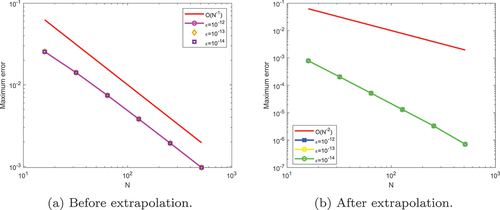
Numerical results in Tables 1–2 for an equal number of mesh points confirm that the present method before extrapolation has been improved after extrapolation for Example (5.1)-(5.2), respectively. Numerical simulation for Examples (5.1)-(5.2) is displayed in Figures 1 and 3, respectively. From these figures, we observe that the formation of twin boundary layers at x = 0 and x = 1 were demonstrated as ɛ and µ goes very small. For a visual understanding of the theoretical order of convergence graphically, the maximum point-wise errors for Examples (5.1)-(5.2) are plotted using log-log scale as can be seen in Figures 2 and 4, respectively showing the $(\mathit{\epsilon },\mathit{\mu })$-uniform convergence.

Table 1. Values of $E_{\epsilon ,\mu ,ext}^{M,\mathrm{\Delta }t},E_{ext}^{M,\mathrm{\Delta }t},R_{ext}^{M,\mathrm{\Delta }t}$, $E_{\epsilon ,\mu }^{M,\mathrm{\Delta }t}$, $E^{\mathit{M},\mathrm{\Delta t}},R^{\mathit{M},\mathrm{\Delta t}}$ for $\mathit{\mu }={10}^{-10}$ fcple (5.1)

$\mathit{\epsilon }\downarrow$	M = 16	32	64	128	256	512
	$\frac{1}{\mathrm{\Delta t}}=16$	32	64	128	256	512
After Extrapolation
10^−12	1.5480e-03	4.2709e-04	1.1287e-04	2.8971e-05	7.2615e-06	1.8206e-06
10^−13	1.5480e-03	4.2709e-04	1.1287e-04	2.8971e-05	7.2615e-06	1.8206e-06
10^−14	1.5480e-03	4.2709e-04	1.1287e-04	2.8971e-05	7.2615e-06	1.8206e-06
10^−15	1.5480e-03	4.2709e-04	1.1287e-04	2.8971e-05	7.2615e-06	1.8206e-06
$E_{ext}^{M,\mathrm{\Delta }t}$	1.5480e-03	4.2709e-04	1.1287e-04	2.8971e-05	7.2615e-06	1.8206e-06
$R_{ext}^{M,\mathrm{\Delta }t}$	1.8578	1.9199	1.9610	1.9963	1.9959	-
Before Extrapolation
10^−12	3.9323e-02	2.1931e-02	1.1594e-02	5.9151e-03	3.0122e-03	1.5200e-03
10^−13	3.9323e-02	2.1931e-02	1.1594e-02	5.9151e-03	3.0122e-03	1.5200e-03
10^−14	3.9323e-02	2.1931e-02	1.1594e-02	5.9151e-03	3.0122e-03	1.5200e-03
10^−15	3.9323e-02	2.1931e-02	1.1594e-02	5.9151e-03	3.0122e-03	1.5200e-03
$E^{\mathit{M},\mathrm{\Delta t}}$	3.9323e-02	2.1931e-02	1.1594e-02	5.9633e-03	3.0122e-03	1.5200e-03
$R^{\mathit{M},\mathrm{\Delta t}}$	0.8424	0.9196	0.9592	0.9795	0.9897	-

Table 2. Values of $E_{\epsilon ,\mu ,ext}^{M,\mathrm{\Delta }t},E_{ext}^{M,\mathrm{\Delta }t},R_{ext}^{M,\mathrm{\Delta }t}$, $E_{\epsilon ,\mu }^{M,\mathrm{\Delta }t}$, $E^{\mathit{M},\mathrm{\Delta t}},R^{\mathit{M},\mathrm{\Delta t}}$ for $\mathit{\mu }={10}^{-10}$ for example (5.2)

$\mathit{\epsilon }\downarrow$	M = 16	32	64	128	256	512
	$\frac{1}{\mathrm{\Delta t}}=16$	32	64	128	256	512
After Extrapolation
10^−12	7.8663e-04	2.0379e-04	5.1861e-05	1.3081e-05	3.2849e-06	7.0877e-07
10^−13	7.8663e-04	2.0379e-04	5.1861e-05	1.3081e-05	3.2849e-06	7.0877e-07
10^−14	7.8663e-04	2.0379e-04	5.1861e-05	1.3081e-05	3.2849e-06	7.0877e-07
10^−15	7.8663e-04	2.0379e-04	5.1861e-05	1.3081e-05	3.2849e-06	7.0877e-07
$E_{ext}^{M,\mathrm{\Delta }t}$	7.8663e-04	2.0379e-04	5.1861e-05	1.3081e-05	3.2849e-06	7.8247e-07
$R_{ext}^{M,\mathrm{\Delta }t}$	1.9486	1.9744	1.9872	1.9936	2.0697	-
Before Extrapolation
10^−12	2.5470e-02	1.4112e-02	7.4251e-03	3.8082e-03	1.9285e-03	9.7038e-04
10^−13	2.5470e-02	1.4112e-02	7.4251e-03	3.8082e-03	1.9285e-03	9.7038e-04
10^−14	2.5470e-02	1.4112e-02	7.4251e-03	3.8082e-03	1.9285e-03	9.7038e-04
10^−15	2.5470e-02	1.4112e-02	7.4251e-03	3.8082e-03	1.9285e-03	9.7038e-04
$E^{\mathit{M},\mathrm{\Delta t}}$	2.5470e-02	1.4112e-02	7.4251e-03	3.8082e-03	1.9285e-03	9.7038e-04
$R^{\mathit{M},\mathrm{\Delta t}}$	0.8519	0.9264	0.9633	0.9816	0.9909	-

Figure 1. Mesh plot of the numerical solution for example (5.1) at $\mathit{M}=32=\frac{1}{\mathrm{\Delta t}}$.

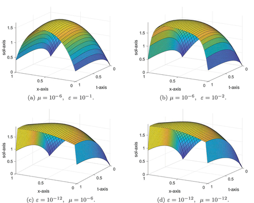
Figure 2. Log-log plot of the maximum errors at $\mathit{\mu }={10}^{-10}$ for example (5.1).

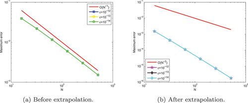
Figure 3. Mesh plot of the numerical solution for example (5.2) at $\mathit{N}=64=\frac{1}{\mathrm{\Delta t}}$.

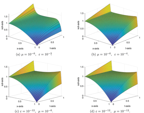
Figure 4. Log-log plot of the maximum errors at $\mathit{\mu }={10}^{-10}$ for example (5.2).

6. Conclusion

From the table of values, we deduce that when the mesh points increase, the maximum point-wise errors decrease. The developed method is first-order uniformly convergent independent of small parameters $\mathit{\epsilon },\mathit{\mu }$. To boost the accuracy, we applied the Richardson extrapolation. Thus, the proposed method is accurate and converges uniformly with order of convergence $\mathit{O}(M^{-1}+\mathrm{\Delta t})$ before extrapolation and $\mathit{O}(M^{-2}+\mathrm{\Delta }{t}^2)$ after extrapolation. The numerical solutions displayed in Tables 1–4 show that the present method is $(\mathit{\epsilon },\mathit{\mu })$-uniformly convergent of second-order and it agrees with the theoretical order of convergence. When ɛ and µ are small, one can see that the proposed method produces smaller errors in Tables 1 and 2 than in Tables 3 and 4. Graphs were plotted for the considered Examples by taking various values of the parameters ɛ and µ to demonstrate the suitability of the proposed method.

Table 3. Values of $E_{\epsilon ,\mu ,ext}^{M,\mathrm{\Delta }t},E_{ext}^{M,\mathrm{\Delta }t},R_{ext}^{M,\mathrm{\Delta }t}$, $E_{\epsilon ,\mu }^{M,\mathrm{\Delta }t}$, $E^{\mathit{M},\mathrm{\Delta t}},R^{\mathit{M},\mathrm{\Delta t}}$ for $\mathit{\epsilon }={10}^{-2}$ for example (5.1)

$\mathit{\mu }\downarrow$	N = 16	32	64	128	256	512
	M = 20	40	80	160	320	640
After Extrapolation
10^−2	1.0488e-01	2.2490e-02	3.9281e-03	8.4280e-04	2.8914e-04	8.1800e-05
10^−3	1.0788e-01	2.3423e-02	4.0687e-03	8.0466e-04	2.6755e-04	7.6925e-05
10^−4	1.0818e-01	2.3521e-02	4.0836e-03	8.0701e-04	2.6522e-04	7.6394e-05
10^−5	1.0821e-01	2.3531e-02	4.0851e-03	8.0724e-04	2.6499e-04	7.6340e-05
10^−6	1.0821e-01	2.3532e-02	4.0853e-03	8.0727e-04	2.6496e-04	7.6335e-05
10^−7	1.0821e-01	2.3532e-02	4.0853e-03	8.0727e-04	2.6496e-04	7.6336e-05
10^−8	1.0821e-01	2.3532e-02	4.0853e-03	8.0727e-04	2.6496e-04	7.6336e-05
$E_{ext}^{M,\mathrm{\Delta }t}$	1.0821e-01	2.3532e-02	4.0853e-03	8.4280e-04	2.8914e-04	8.1800e-05
$R_{ext}^{M,\mathrm{\Delta }t}$	2.2011	2.5261	2.3393	1.6073	1.7953	-
Before Extrapolation
10^−2	1.8154e-01	1.3967e-01	7.7731e-02	3.8898e-02	1.9136e-02	9.4482e-03
10^−3	1.7976e-01	1.4068e-01	7.9074e-02	3.9784e-02	1.9626e-02	9.7032e-03
10^−4	1.7956e-01	1.4077e-01	7.9203e-02	3.9871e-02	1.9674e-02	9.7286e-03
10^−5	1.7954e-01	1.4077e-01	7.9216e-02	3.9880e-02	1.9679e-02	9.7311e-03
10^−6	1.7953e-01	1.4077e-01	7.9217e-02	3.9881e-02	1.9680e-02	9.7314e-03
10^−7	1.7953e-01	1.4077e-01	7.9217e-02	3.9881e-02	1.9680e-02	9.7314e-03
10^−8	1.7953e-01	1.4077e-01	7.9217e-02	3.9881e-02	1.9680e-02	9.7314e-03
$E^{\mathit{M},\mathrm{\Delta t}}$	1.8154e-01	1.4077e-01	7.9217e-02	3.9881e-02	1.9680e-02	9.7314e-03
$R^{\mathit{M},\mathrm{\Delta t}}$	0.3509	0.8295	0.9901	1.0190	1.0160	-

Table 4. Values of $E_{\epsilon ,\mu ,ext}^{M,\mathrm{\Delta }t},E_{ext}^{M,\mathrm{\Delta }t},R_{ext}^{M,\mathrm{\Delta }t}$, $E_{\epsilon ,\mu }^{M,\mathrm{\Delta }t}$, $E^{\mathit{M},\mathrm{\Delta t}},R^{\mathit{M},\mathrm{\Delta t}}$ for $\mathit{\epsilon }={10}^{-2}$ for example (5.2)

$\mathit{\mu }\downarrow$	M = 16	32	64	128	256	512
	$\frac{1}{\mathrm{\Delta t}}=20$	40	80	160	320	640
After Extrapolation
10^−2	5.7253e-02	3.1148e-02	9.3911e-03	2.3557e-03	5.7327e-04	1.4028e-04
10^−3	6.0496e-02	3.0266e-02	9.1425e-03	2.2985e-03	5.6028e-04	1.3724e-04
10^−4	6.0816e-02	3.0179e-02	9.1179e-03	2.2929e-03	5.5899e-04	1.3694e-04
10^−5	6.0848e-02	3.0170e-02	9.1154e-03	2.2923e-03	5.5886e-04	1.3691e-04
10^−6	6.0852e-02	3.0169e-02	9.1152e-03	2.2922e-03	5.5885e-04	1.3690e-04
10^−7	6.0852e-02	3.0169e-02	9.1152e-03	2.2922e-03	5.5885e-04	1.3690e-04
10^−8	6.0852e-02	3.0169e-02	9.1152e-03	2.2922e-03	5.5885e-04	1.3690e-04
$E_{ext}^{M,\mathrm{\Delta }t}$	6.0852e-02	3.1148e-02	9.3911e-03	2.3557e-03	5.7327e-04	1.4028e-04
$R_{ext}^{M,\mathrm{\Delta }t}$	0.9662	1.7298	1.9951	2.0389	2.0309	-
Before Extrapolation
10^−2	1.1838e-01	8.7818e-02	4.7173e-02	2.3095e-02	1.2005e-02	6.2891e-03
10^−3	1.1760e-01	8.9047e-02	4.8449e-02	2.3884e-02	1.1679e-02	6.1196e-03
10^−4	1.1750e-01	8.9159e-02	4.8573e-02	2.3962e-02	1.1696e-02	6.1029e-03
10^−5	1.1749e-01	8.9170e-02	4.8585e-02	2.3970e-02	1.1700e-02	6.1012e-03
10^−6	1.1749e-01	8.9171e-02	4.8586e-02	2.3971e-02	1.1701e-02	6.1010e-03
10^−7	1.1749e-01	8.9171e-02	4.8586e-02	2.3971e-02	1.1701e-02	6.1010e-03
10^−8	1.1749e-01	8.9171e-02	4.8586e-02	2.3971e-02	1.1701e-02	6.1010e-03
$E^{\mathit{M},\mathrm{\Delta t}}$	1.1838e-01	8.9171e-02	4.8586e-02	2.3971e-02	1.2005e-02	6.2891e-03
$R^{\mathit{M},\mathrm{\Delta }\mathit{t}}$	0.4088	0.8760	1.0193	0.9977	0.9327	-

Public Interest Statement

Asymptotic and numerical solutions to two-parameter singularly perturbed differential equations have received relatively little study in comparison to their one-parameter counterparts. Various numerical approaches for solving singularly perturbed parabolic two-parameters problems with initial-Dirichlet boundary conditions have recently been developed. In this study, a non-standard fitted operator method in the space direction and implicit Euler method in the time direction are used to discretize a singularly perturbed parabolic two-parameters problems with initial-Robin boundary conditions. Furthermore, the new fitted operator method is used to discretize the Robin boundary conditions. The present method with Richardson extrapolation gives more accurate, stable, and uniformly convergent numerical solutions.

Acknowledgements

The authors are thanks the anonymous reviewers for their constructive comments and suggestions aimed at improving the quality of the manuscript.

Disclosure statement

No potential conflict of interest was reported by the author(s).

Funding

The authors received no direct funding for this research work.

Supplementary Material

Supplemental data for this article can be accessed online at https://doi.org/10.1080/27684830.2024.2354536

Additional information

Notes on contributors

Fasika Wondimu Gelu

Fasika Wondimu Gelu received his M.Sc. and Ph.D. degrees from the Department of Mathematics, Jimma University, Ethiopia. Since 2016 he has been a lecturer at Dilla University, Ethiopia. He is the author of (13) thirteen articles published in different national and international journals. The authors of this research work have focused on numerical solution of singularly perturbed problems of ODEs and PDEs with one-parameter and two-parameters.

Gemechis File Duressa

Gemechis File Duressa received his M.Sc. degree from Addis Ababa University, Ethiopia, and a Ph.D. degree from National Institute of Technology, Warangal, India. He is presently working at Jimma University as a full Professor of Mathematics and Vice President, administrative and development, Jimma University, Ethiopia. He is the author of more than 185 research papers published in different national and international journals. He is working as a referee for several reputable international journals. The authors of this research work have focused on numerical solution of singularly perturbed problems of ODEs and PDEs with one-parameter and two-parameters.

References

- Bhathawala, P. H., & Verma, A. P. (1975). A two-parameter singular perturbation solution of one dimension flow through unsaturated porous media. Proceedings of the Indian National Science Academy, 43(5), 380–384.
- Bigge, J., & Bohl, E. (1985). Deformations of the bifurcation diagram due to discretization. Mathematics of Computation, 45(172), 393–403. http://dx.doi.org/10.1090/S0025-5718-1985-0804931-X
- Bullo, T. A., Degla, G. A., & Duressa, G. F. (2022). Parameter-uniform finite difference method for singularly perturbed parabolic problem with two small parameters. International Journal for Computational Methods in Engineering Sciences and Mechanics, 23(3), 210–218. https://doi.org/10.1080/15502287.2021.1948148
- Bullo, T. A., Duressa, G. F., & Delga, G. A. (2021a). A parameter-uniform finite difference scheme for singularly perturbed parabolic problem with two small parameters. European Journal of Computational Mechanics, 30(2–3), 197–222. https://doi.org/10.13052/ejcm2642-2085.30233
- Bullo, T. A., Duressa, G. F., & Delga, G. A. (2021b). Robust finite difference method for singularly perturbed two-parameter parabolic convection-diffusion problems. International Journal of Computational Methods, 18(2), 2050034. https://doi.org/10.1142/S0219876220500346
- Chandru, M., Das, P., & Ramos, H. (2018). Numerical treatment of two-parameter singularly perturbed parabolic convection diffusion problems with non-smooth data. Mathematical Methods in the Applied Sciences, 41(14), 5359–5387. https://doi.org/10.1002/mma.5067
- Chandru, M., Prabha, T., Das, P., & Shanthi, V. (2019). A numerical method for solving boundary and interior layers dominated parabolic problems with discontinuous convection coefficient and source terms. Differential Equations and Dynamical Systems, 27(1–3), 91–112. https://doi.org/10.1007/s12591-017-0385-3
- Chen, J., & O’Malley, R. E., Jr. (1974). On the asymptotic solution of a two-parameter boundary value problem of chemical reactor theory. SIAM Journal of Applied Mathematics, 26(4), 717–729. https://doi.org/10.1137/0126064
- Daba, I. T., Duressa, G. F., & Liu, L. (2022). A novel algorithm for singularly perturbed parabolic differential-difference equations. Research in Mathematics, 9(1), 2133211. https://doi.org/10.1080/27684830.2022.2133211
- Das, P. (2018). A higher order difference method for singularly perturbed parabolic partial differential equations. Journal of Difference Equations and Applications, 24(3), 452–477. https://doi.org/10.1080/10236198.2017.1420792
- Das, P., & Mehrmann, V. (2016). Numerical solution of singularly perturbed convection-diffusion-reaction problems with two small parameters. BIT Numerical Mathematics, 56(1), 51–76. https://doi.org/10.1007/s10543-015-0559-8
- Das, P., & Natesan, S. (2013a). Richardson extrapolation method for singularly perturbed convection-diffusion problems on adaptively generated mesh. CMES, 90(6), 463–485. https://doi.org/10.3970/cmes.2013.090.463.html
- Das, P., & Natesan, S. (2013b). A uniformly convergent hybrid scheme for singularly perturbed system of reaction-diffusion Robin type boundary-value problems. Journal of Applied Mathematics and Computing, 41(1–2), 447–471. https://doi.org/10.1007/s12190-012-0611-7
- Das, P., Rana, S., & Vigo-Aguiar, J. (2020). Higher order accurate approximations on equidistributed meshes for boundary layer originated mixed type reaction diffusion systems with multiple scale nature. Applied Numerical Mathematic, 148, 79–97. https://doi.org/10.1016/j.apnum.2019.08.028
- DiPrima, R. C. (1968). Asymptotic methods for an infinitely long slider squeeze-film bearing. Journal of Lubrication Technology, 90(1), 173–183. https://doi.org/10.1115/1.3601534
- Duressa, G. F., Gelu, F. W., & Kebede, G. D. (2023). A robust higher-order fitted mesh numerical method for solving singularly perturbed parabolic reaction-diffusion problems. Results in Applied Mathematics, 20, 100405. https://doi.org/10.1016/j.rinam.2023.100405
- Gelu, F. W., & Duress, G. F. (2022). Parameter-uniform numerical scheme for singularly perturbed parabolic convection-diffusion Robin type problems with a boundary turning point. Results in Applied Mathematics, 15(2), 100324. https://doi.org/10.1016/j.rinam.2022.100324
- Gelu, F. W., & Duressa, G. F. (2022a). Computational method for singularly perturbed parabolic reaction-diffusion equations with Robin boundary conditions. Journal of Applied Mathematics & Informatics, 40(1–2), 25–45. https://doi.org/10.14317/jami.2022.025
- Gelu, F. W., & Duressa, G. F. (2023a). Hybrid method for singularly perturbed Robin type parabolic convection–diffusion problems on Shishkin mesh. Partial Differential Equations in Applied Mathematics, 8, 100586. https://doi.org/10.1016/j.padiff.2023.100586
- Gelu, F. W., & Duressa, G. F. (2023b). A parameter-uniform numerical method for singularly perturbed Robin type parabolic convection-diffusion turning point problems. Applied Numerical Mathematics, 190, 50–64. https://doi.org/10.1016/j.apnum.2023.04.007
- Gelu, F. W., Duressa, G. F., & Kovtunenko, V. (2021). A uniformly convergent collocation method for singularly perturbed delay parabolic reaction-diffusion problems. Abstract and Applied Analysis, 2021, 1–11. https://doi.org/10.1155/2021/8835595
- Gelu, F. W., Duressa, G. F., & Shah, F. A. (2022b). A novel numerical approach for singularly perturbed parabolic convection-diffusion problems on layer-adapted meshes. Research in Mathematics, 9(1), 2020400. https://doi.org/10.1080/27658449.2021.2020400
- Gupta, V., Kadalbajoo, M. K., & Dubey, R. K. (2019). A parameter-uniform higher order finite difference scheme for singularly perturbed time-dependent parabolic problem with two small parameters. International Journal of Computer Mathematics, 96(3), 474–499. https://doi.org/10.1080/00207160.2018.1432856
- Hailu, W. S., Duressa, G. F., & Liu, L. (2022a). Parameter-uniform cubic spline method for singularly perturbed parabolic differential equation with large negative shift and integral boundary condition. Research in Mathematics, 9(1), 2151080. https://doi.org/10.1080/27684830.2022.2151080
- Hailu, W. S., Duressa, G. F., & Liu, L. (2022b). Uniformly convergent numerical method for singularly perturbed parabolic differential equations with non-smooth data and large negative shift. Research in Mathematics, 9(1), 2119677. https://doi.org/10.1080/27684830.2022.2119677
- Hassen, Z. I., Duressa, G. F., & Liu, L. (2023). New approach of convergent numerical method for singularly perturbed delay parabolic convection-diffusion problems. Research in Mathematics, 10(1), 2225267. https://doi.org/10.1080/27684830.2023.2225267
- Hemker, P. W., Shishkin, G. I., & Shishkina, L. P. (2002). High-order time-accurate schemes for singularly perturbed parabolic convection-diffusion problems with Robin boundary conditions. Computational Methods in Applied Mathematics, 2(1), 3–25. https://doi.org/10.2478/cmam-2002-0001
- Janani Jayalakshmi, G., & Tamilselvan, A. (2020). An ɛ-uniform method for a class of singularly perturbed parabolic problems with Robin boundary conditions having boundary turning point. Asian-European Journal of Mathematics, 13(1), 2050025. https://doi.org/10.1142/S1793557120500254
- Jha, A., & Kadalbajoo, M. K. (2015). A robust layer adapted difference method for singularly perturbed two-parameter parabolic problems. International Journal of Computer Mathematics, 92(6), 1204–1221. https://doi.org/10.1080/00207160.2014.928701
- Kadalbajoo, M. K., & Yadaw, A. S. (2012). Parameter-uniform finite element method for two-parameter singularly perturbed parabolic reaction-diffusion problems. International Journal of Computational Methods, 09(4), 1250047–1)-(1250047–16. https://doi.org/10.1142/S0219876212500478
- Kumar, D., & Deswal, K. (2022). Wavelet-based approximation for two-parameter singularly perturbed problems with Robin boundary conditions. Journal of Applied Mathematics and Computing, 68(1), 125–149. https://doi.org/10.1007/s12190-021-01511-2
- Kumar, S., Aakansha, S. J., & Ramos, H. (2023). Parameter-uniform convergence analysis of a domain decomposition method for singularly perturbed parabolic problems with Robin boundary conditions. Journal of Applied Mathematics and Computing, 69, 2239–2261. https://doi.org/10.1007/s12190-022-01832-w
- Mbroh, N. A., Noutchie, S. C. O., & Massoukou, R. Y. M. (2020). A uniformly convergent finite difference scheme for Robin type singularly perturbed parabolic convection diffusion problem. Mathematics and Computers in Simulation, 174, 218–232. https://doi.org/10.1016/j.matcom.2020.03.003
- Mekonnen, T. B., Duressa, G. F., & Liu, L. (2020). Computational method for singularly perturbed two-parameter parabolic convection-diffusion problems. Cogent Mathematics & Statistics, 7(1), 1829277. https://doi.org/10.1080/25742558.2020.1829277
- Mekonnen, T. B., Duressa, G. F., & Liu, L. (2021). Uniformly convergent numerical method for two-parametric singularly perturbed parabolic convection-diffusion problems. Journal of Applied and Computational Mechanics, 7(1), 1829277–1829545. https://doi.org/10.1080/25742558.2020.1829277
- Mickens, R. E. (1994). Nonstandard finite difference models of differential equations. World Scientific.
- Mickens, R. E. (2005). Advances in the applications of nonstandard finite difference schemes. World Scientific.
- Munyakazi, J. B. (2015). A robust finite difference method for two-parameter parabolic convection-diffusion problems. Applied Mathematics and Information Sciences, 9(6), 2877–2883. https://doi.org/10.12785/amis/090614
- O’Malley, R. E., Jr. (1967a). Singular perturbations of boundary value problems for linear ordinary differential equations involving two-parameters. Journal of Mathematical Analysis and Applications, 19(2), 291–308. https://doi.org/10.1016/0022-247X(67)90124-2
- O’Malley, R. E., Jr. (1967b). Two-parameter singular perturbation problems for second-order equations. Journal of Mathematics and Mechanics, 16(10), 1143–1164. https://www.jstor.org/stable/45277141
- O’Malley, R. E., Jr. (1969). Boundary value problems for linear systems of ordinary differential equations involving many small parameters. Journal of Mathematics and Mechanics, 18, 835–856. https://www.jstor.org/stable/24901722
- O’Riordan, E., Pickett, M. L., & Shishkin, G. I. (2006). Parameter-uniform finite difference schemes for singularly perturbed parabolic diffusion-convection-reaction problems. Mathematics of Computation, 75(255), 1135–1154. https://doi.org/10.1090/S0025-5718-06-01846-1
- Patidar, K. C. (2008). A robust fitted operator finite difference method for a two-parameter singular perturbation problem 1. Journal of Difference Equations and Applications, 14(12), 1197–1214. https://doi.org/10.1080/10236190701817383
- Patidar, K. C., & Sharma, K. K. (2006). Uniformly convergent nonstandard finite difference methods for singularly perturbed differential-difference equations with delay and advance. International Journal Numerical Methods in Engineering, 66(2), 272–296. https://doi.org/10.1002/nme.1555
- Saini, S., Das, P., & Kumar, S. (2023). Computational cost reduction for coupled system of multiple scale reaction diffusion problems with mixed type boundary conditions having boundary layers. Revista de la Real Academia de Ciencias Exactas, Físicas y Naturales, Serie A Matemáticas, 117(2), 66. https://doi.org/10.1007/s13398-023-01397-8
- Saini, S., Das, P., & Kumar, S. (2024). Parameter uniform higher order numerical treatment for singularly perturbed Robin type parabolic reaction diffusion multiple scale problems with large delay in time. Applied Numerical Mathematics, 196, 1–21. https://doi.org/10.1016/j.apnum.2023.10.003
- Selvi, P. A., & Ramanujam, N. (2017). A parameter uniform difference scheme for singularly perturbed parabolic delay differential equation with Robin type boundary condition. Applied Mathematics and Computation, 296, 101–115. https://doi.org/10.1016/j.amc.2016.10.027
- Srivastava, H. M., Nain, A. K., Vats, R. K., & Das, P. (2023). A theoretical study of the fractional-order p-Laplacian nonlinear Hadamard type turbulent flow models having the Ulam–Hyers stability. Revista de la Real Academia de Ciencias Exactas, Físicas Y Naturales, Serie A Matemáticas, 117(4), 160. https://doi.org/10.1007/s13398-023-01488-6
- Sumit, K., Kuldeep, S., & Kumar, M. (2020). A robust numerical method for a two-parameter singularly perturbed time delay parabolic problem. Computational and Applied Mathematics, 39, 209. https://doi.org/10.1007/s40314-020-01236-1
- Sunil, K., Sumit, & Ramos, H. (2021). Parameter-uniform approximation on equidistributed meshes for singularly perturbed parabolic reaction-diffusion problems with Robin boundary conditions. Applied Mathematics Computation, 392, 125677. https://doi.org/10.1016/j.amc.2020.125677
- Vasil’eva, A. B. (1963). Asymptotic methods in the theory of ordinary differential equations containing small parameters in front of the highest derivatives. USSR Computational Mathematics and Mathematical Physics, 3(4), 823–863. https://doi.org/10.1016/0041-5553(63)90381-1