Asymptotic series solution of variational stokes problems in planar domain with crack-like singularity

ABSTRACT

A class of nonlinear variational problems describing incompressible fluids and solids by stationary Stokes equations given in a planar domain with a crack (infinitely thin flat plate in fluids) is considered. Based on the Fourier asymptotic analysis, general analytical solutions are obtained in polar coordinates as the power series with respect to the distance to the crack tip. The logarithm terms and angular functions are accounted in the asymptotic expansion using recurrence relations. Then boundary conditions imposed between the opposite crack faces in the sector of angle $2\pi$ determine admissible exponents and parameters in the power series. For the specific conditions of Dirichlet, Neumann, impermeability, non-penetration and shear crack, the principal asymptotic terms are derived, which verify the singular behaviour. In particular, the analytical solution answers the questions of a square-root singularity at the crack tip and the presence of log-oscillations of variational solutions for the Stokes problems.

KEYWORDS:

• Stokes system
• incompressibility
• mixed variational problem
• asymptotic theory
• Fourier analysis
• power series
• recurrence relation
• crack
• non-penetration
• crack-tip singularity

AMS CLASSIFICATIONS:

• 35Q30
• 35C10
• 74A50

1. Introduction

The Stokes system can describe stationary flow of incompressible fluids [1] as well as incompressible linearly elastic solids that are subject to the divergence-free condition [2]. We refer to suitable qualitative properties of solutions given in Ref. [3] and related regularity results in Ref. [4,5] for dual strategies solving the Stokes problem. Motivated by applications to fracture mechanics, in our study we are interested in the presence of a crack in a reference domain (see the variational theory of crack problems in the monograph by Khludnev and Kovtunenko [6]). For fluids, the discontinuity may be suitable when simplifying aeroplane wings to infinitely thin flat plates. This research has further important extensions to nonlinear continuum mechanics [7,8], shape optimization [9–11], overdetermined [12] and inverse problems [13].

The main question of crack problems consists in finding a singularity at the crack tip. The generic singularity is of power type with respect to the distance to the crack tip and may contain logarithmic terms, whose presence or absence is of especial importance for engineers. If we consider linear elastic boundary value problems for cracked configurations, then we have the Williams series solution [14]. The boundary value problems analyzed in the paper have long history. Highlighting questions related to the singularity in the vicinity of the crack we cite [15], the respective approaches use regular and singular perturbations [16–18], integral Fourier and Mellin transforms [19]. Here we focus on asymptotic series solution for incompressible continua given in a planar domain corresponding to the sector of angle $2\pi$.

The crack singularities for general elliptic systems in planar domains were analyzed in Ref. [20] in dependence of boundary conditions. Thus, the Lamé system describing isotropic bodies with a stress-free crack (the homogeneous Neumann boundary condition) obeys the classic square-root singularity without logarithms. It is worth noting that Stokes equations correspond to the limit case of the Lamé equations when the Poisson ratio $\nu \to 0.5$ (hence the Lamé parameter $\lambda \to \mathrm{\infty }$). Setting $\nu =0.5$ in asymptotic formulas was suggested in Ref. [21] to get the displacement appropriate for the special case of an incompressible body. However, in the limit state of Stokes equations under non-penetration conditions, log-oscillations may occur for high-order asymptotic terms. In Ref. [22, Chapters 5 and 6], Stokes problems in conical domains were investigated with respect to its eigenvalues and generalized eigenvalues generated by Dirichlet and Neumann conditions.

Commonly, boundary conditions are incorporated into the operator pencil for differential equations in order to determine admissible exponents and parameters in the power series after solving this eigenvalue problem [3,4,20,22]. This approach is highly dependent on the specific choice of conditions imposed on the boundary. In contrast, we obtain first a general asymptotic solution for the Stokes equations using Fourier asymptotic expansion and recurrence relations for logarithmic terms and angular functions. Then we can specify coefficients in the power series for every kind of boundary conditions imposed between the opposite crack faces, even for nonlinear ones. For engineers, it is important to note that we establish: if log-oscillations occur in the power series, or not. In this way, we provide the principal asymptotic terms for the condition of Dirichlet, Neumann, impermeability, non-penetration and shear crack presented next.

In the domain with crack ${\mathrm{\Omega }}_{\text{c}}$, let unknown displacement (velocity for fluids) vector $\mathbf{u}$ and scalar pressure p satisfy the homogeneous Stokes equations: (1) $\begin{array}{r}-\mu \mathrm{\Delta }\mathbf{u}+\mathrm{\nabla }p=\mathbf{0},\text{div}\mathbf{u}=0,\end{array}$(1) where the shear modulus $\mu =E/3$ and Young's modulus E>0. This constitutes the Cauchy stress $\mathit{\tau }$ in terms of the linearized strain $\mathit{\epsilon }$ and pressure p as (2) $\begin{array}{r}\mathit{\tau }=2\mu \mathit{\epsilon }(\mathbf{u})-p\mathbf{I},\mathit{\epsilon }(\mathbf{u})=\frac{1}{2}(\mathrm{\nabla }\mathbf{u}+\mathrm{\nabla }{\mathbf{u}}^{\mathrm{\top }}),\end{array}$(2) where $\mathbf{I}$ is the identity transformation. At the crack ${\mathrm{\Gamma }}_{\text{c}}$ with a normal vector $\mathbf{n}$, we can distinguish traces of the discontinuous functions $\mathbf{u}$, $\mathit{\tau }$, and p across the opposite crack faces ${\mathrm{\Gamma }}_{\text{c}}^{\pm }$, thus the jump: (3) $\begin{array}{r}[[\mathbf{u}]]:=\mathbf{u}{|}_{{\mathrm{\Gamma }}_{\text{c}}^{+}}-\mathbf{u}{|}_{{\mathrm{\Gamma }}_{\text{c}}^{-}},[[\mathit{\tau }]]:=\mathit{\tau }{|}_{{\mathrm{\Gamma }}_{\text{c}}^{+}}-\mathit{\tau }{|}_{{\mathrm{\Gamma }}_{\text{c}}^{-}},[[p]]:=p{|}_{{\mathrm{\Gamma }}_{\text{c}}^{+}}-p{|}_{{\mathrm{\Gamma }}_{\text{c}}^{-}},\end{array}$(3) and the mean: (4) $\begin{array}{r}\{\{\mathbf{u}\}\}:=\frac{1}{2}(\mathbf{u}{|}_{{\mathrm{\Gamma }}_{\text{c}}^{+}}+\mathbf{u}{|}_{{\mathrm{\Gamma }}_{\text{c}}^{-}}),\{\{\mathit{\tau }\}\}:=\frac{1}{2}(\mathit{\tau }{|}_{{\mathrm{\Gamma }}_{\text{c}}^{+}}+\mathit{\tau }{|}_{{\mathrm{\Gamma }}_{\text{c}}^{-}}),\{\{p\}\}:=\frac{1}{2}(p{|}_{{\mathrm{\Gamma }}_{\text{c}}^{+}}+p{|}_{{\mathrm{\Gamma }}_{\text{c}}^{-}}).\end{array}$(4) Using (2(2) $\begin{array}{r}\mathit{\tau }=2\mu \mathit{\epsilon }(\mathbf{u})-p\mathbf{I},\mathit{\epsilon }(\mathbf{u})=\frac{1}{2}(\mathrm{\nabla }\mathbf{u}+\mathrm{\nabla }{\mathbf{u}}^{\mathrm{\top }}),\end{array}$(2) )–(4(4) $\begin{array}{r}\{\{\mathbf{u}\}\}:=\frac{1}{2}(\mathbf{u}{|}_{{\mathrm{\Gamma }}_{\text{c}}^{+}}+\mathbf{u}{|}_{{\mathrm{\Gamma }}_{\text{c}}^{-}}),\{\{\mathit{\tau }\}\}:=\frac{1}{2}(\mathit{\tau }{|}_{{\mathrm{\Gamma }}_{\text{c}}^{+}}+\mathit{\tau }{|}_{{\mathrm{\Gamma }}_{\text{c}}^{-}}),\{\{p\}\}:=\frac{1}{2}(p{|}_{{\mathrm{\Gamma }}_{\text{c}}^{+}}+p{|}_{{\mathrm{\Gamma }}_{\text{c}}^{-}}).\end{array}$(4) ), we set the following boundary conditions at ${\mathrm{\Gamma }}_{\text{c}}$ for the stick (homogeneous Dirichlet): (5) $\begin{array}{r}[[\mathbf{u}]]=\{\{\mathbf{u}\}\}=\mathbf{0},\end{array}$(5) impermeability (mixed homogeneous Dirichlet–Neumann): (6) $\begin{array}{r}[[\mathbf{u}\cdot \mathbf{n}]]=\{\{\mathbf{u}\cdot \mathbf{n}\}\}=0,[[\mathit{\tau }-(\mathit{\tau }\cdot \mathbf{n})\mathbf{n}]]=\{\{\mathit{\tau }-(\mathit{\tau }\cdot \mathbf{n})\mathbf{n}\}\}=\mathbf{0},\end{array}$(6) stress-free crack (homogeneous Neumann): (7) $\begin{array}{r}[[\mathit{\tau }]]=\{\{\mathit{\tau }\}\}=\mathbf{0},\end{array}$(7) non-penetration (complementarity): (8) $\begin{array}{rl}[[\mathit{\tau }-(\mathit{\tau }\cdot \mathbf{n})\mathbf{n}]]& =\{\{\mathit{\tau }-(\mathit{\tau }\cdot \mathbf{n})\mathbf{n}\}\}=\mathbf{0},[[\mathit{\tau }\cdot \mathbf{n}]]=0,[[\mathbf{u}\cdot \mathbf{n}]]\ge 0,\\ \mathit{\tau }\cdot \mathbf{n}& \le 0,[[\mathbf{u}\cdot \mathbf{n}]](\mathit{\tau }\cdot \mathbf{n})=0,\end{array}$(8) and shear crack (transmission with slip): (9) $\begin{array}{r}[[\mathit{\tau }-(\mathit{\tau }\cdot \mathbf{n})\mathbf{n}]]=\{\{\mathit{\tau }-(\mathit{\tau }\cdot \mathbf{n})\mathbf{n}\}\}=\mathbf{0},[[\mathit{\tau }\cdot \mathbf{n}]]=[[\mathbf{u}\cdot \mathbf{n}]]=0.\end{array}$(9) The power series solution for the Stokes equation (1(1) $\begin{array}{r}-\mu \mathrm{\Delta }\mathbf{u}+\mathrm{\nabla }p=\mathbf{0},\text{div}\mathbf{u}=0,\end{array}$(1) ) when expressed in polar $(r,\theta )$-coordinates is found in the general form of sum (10) $\begin{array}{rl}\mathbf{u}(r,\theta )& =\sum _{\gamma \in \mathbb{R}}{r}^{\gamma }\sum _{m=0}^{M(\gamma )}\frac{(\ln r{)}^{M(\gamma )-m}}{(M(\gamma )-m)!}{\mathbf{\Psi }}^m(\gamma ,\theta ),\\ p(r,\theta )& =\sum _{\gamma \in \mathbb{R}}{r}^{\gamma -1}\sum _{m=0}^{M(\gamma )}\frac{(\ln r{)}^{M(\gamma )-m}}{(M(\gamma )-m)!}{\mathrm{\Phi }}^m(\gamma ,\theta ),\end{array}$(10) where the angular functions are determined by the recurrence relations for $m=1,\dots ,M(\gamma )$: (11) $\begin{array}{rl}{\mathbf{\Psi }}^0& =\sum _{l=1}^4{U}_l^0{\mathit{\psi }}_l(\gamma ,\theta ),{\mathbf{\Psi }}^m=\sum _{l=1}^4{U}_l^m{\mathit{\psi }}_l(\gamma ,\theta )-\sum _{i=1}^m\frac{(-1{)}^i}{i!}\frac{{\mathrm{\partial }}^i{\mathbf{\Psi }}^{m-i}}{\mathrm{\partial }{\gamma }^i},\end{array}$(11) (12) $\begin{array}{rl}{\mathrm{\Phi }}^0& =\sum _{l=1}^4{P}_l^0{\varphi }_l(\gamma ,\theta ),{\mathrm{\Phi }}^m=\sum _{l=1}^4{P}_l^m{\varphi }_l(\gamma ,\theta )-\sum _{i=1}^m\frac{(-1{)}^i}{i!}\frac{{\mathrm{\partial }}^i{\mathrm{\Phi }}^{m-i}}{\mathrm{\partial }{\gamma }^i},\end{array}$(12) with free coefficients $U_l^m,P_l^m\in \mathbb{R}$. The four eigenvectors ${\mathit{\psi }}_1,\dots ,{\mathit{\psi }}_4$ and ${\varphi }_1,\dots ,{\varphi }_4$ (where ${\varphi }_1={\varphi }_2=0$) of the operator pencil are found from the condition that for every $l=1,\dots ,4$ functions ${\mathbf{u}}^{\gamma }=r^{\gamma }{\mathit{\psi }}_l$ and $p^{\gamma }=r^{\gamma -1}{\varphi }_l$ solve the homogeneous Stokes equation (1(1) $\begin{array}{r}-\mu \mathrm{\Delta }\mathbf{u}+\mathrm{\nabla }p=\mathbf{0},\text{div}\mathbf{u}=0,\end{array}$(1) ).

Inserting ansatz (10(10) $\begin{array}{rl}\mathbf{u}(r,\theta )& =\sum _{\gamma \in \mathbb{R}}{r}^{\gamma }\sum _{m=0}^{M(\gamma )}\frac{(\ln r{)}^{M(\gamma )-m}}{(M(\gamma )-m)!}{\mathbf{\Psi }}^m(\gamma ,\theta ),\\ p(r,\theta )& =\sum _{\gamma \in \mathbb{R}}{r}^{\gamma -1}\sum _{m=0}^{M(\gamma )}\frac{(\ln r{)}^{M(\gamma )-m}}{(M(\gamma )-m)!}{\mathrm{\Phi }}^m(\gamma ,\theta ),\end{array}$(10) )–(12(12) $\begin{array}{rl}{\mathrm{\Phi }}^0& =\sum _{l=1}^4{P}_l^0{\varphi }_l(\gamma ,\theta ),{\mathrm{\Phi }}^m=\sum _{l=1}^4{P}_l^m{\varphi }_l(\gamma ,\theta )-\sum _{i=1}^m\frac{(-1{)}^i}{i!}\frac{{\mathrm{\partial }}^i{\mathrm{\Phi }}^{m-i}}{\mathrm{\partial }{\gamma }^i},\end{array}$(12) ) into the boundary conditions (5(5) $\begin{array}{r}[[\mathbf{u}]]=\{\{\mathbf{u}\}\}=\mathbf{0},\end{array}$(5) )–(9(9) $\begin{array}{r}[[\mathit{\tau }-(\mathit{\tau }\cdot \mathbf{n})\mathbf{n}]]=\{\{\mathit{\tau }-(\mathit{\tau }\cdot \mathbf{n})\mathbf{n}\}\}=\mathbf{0},[[\mathit{\tau }\cdot \mathbf{n}]]=[[\mathbf{u}\cdot \mathbf{n}]]=0.\end{array}$(9) ) as $\theta =\pi$ and $\theta =-\pi$, for every condition we determine the admissible eigenvalues γ, the presence of generalized eigenvectors by means of $M(\gamma )$, and coefficients $U_1^m,\dots ,U_4^m,P_3^m,P_4^m$ for $m=0,1,\dots$. The important observation is that, if only trivial ${\mathbf{\Psi }}^0=\mathbf{0}$ and ${\mathrm{\Phi }}^0=0$ are possible in (11(11) $\begin{array}{rl}{\mathbf{\Psi }}^0& =\sum _{l=1}^4{U}_l^0{\mathit{\psi }}_l(\gamma ,\theta ),{\mathbf{\Psi }}^m=\sum _{l=1}^4{U}_l^m{\mathit{\psi }}_l(\gamma ,\theta )-\sum _{i=1}^m\frac{(-1{)}^i}{i!}\frac{{\mathrm{\partial }}^i{\mathbf{\Psi }}^{m-i}}{\mathrm{\partial }{\gamma }^i},\end{array}$(11) ) and (12(12) $\begin{array}{rl}{\mathrm{\Phi }}^0& =\sum _{l=1}^4{P}_l^0{\varphi }_l(\gamma ,\theta ),{\mathrm{\Phi }}^m=\sum _{l=1}^4{P}_l^m{\varphi }_l(\gamma ,\theta )-\sum _{i=1}^m\frac{(-1{)}^i}{i!}\frac{{\mathrm{\partial }}^i{\mathrm{\Phi }}^{m-i}}{\mathrm{\partial }{\gamma }^i},\end{array}$(12) ), then ${\mathbf{\Psi }}^1=\mathbf{0}$ and ${\mathrm{\Phi }}^1=0$ too, thus $M(\gamma )=0$, and there is no logarithms. Otherwise, if non-trivial ${\mathbf{\Psi }}^0,{\mathrm{\Phi }}^0,{\mathbf{\Psi }}^1,{\mathrm{\Phi }}^1$ exist, then natural number $M(\gamma )\ge 1$ may be arbitrary.

The energy $H^1$-solution $\mathbf{u}$ excepting possible constant $\mathbf{u}(\mathbf{0})$ restricts to $\gamma >0$. In particular, we found the crack-tip singular of energy solutions (the principal asymptotic terms) according to the following expansions as $r\to \mathrm{\infty }$ for the boundary conditions of Dirichlet (5(5) $\begin{array}{r}[[\mathbf{u}]]=\{\{\mathbf{u}\}\}=\mathbf{0},\end{array}$(5) ), mixed Dirichlet–Neumann (6(6) $\begin{array}{r}[[\mathbf{u}\cdot \mathbf{n}]]=\{\{\mathbf{u}\cdot \mathbf{n}\}\}=0,[[\mathit{\tau }-(\mathit{\tau }\cdot \mathbf{n})\mathbf{n}]]=\{\{\mathit{\tau }-(\mathit{\tau }\cdot \mathbf{n})\mathbf{n}\}\}=\mathbf{0},\end{array}$(6) ), Neumann (7(7) $\begin{array}{r}[[\mathit{\tau }]]=\{\{\mathit{\tau }\}\}=\mathbf{0},\end{array}$(7) ) and non-penetration (8(8) $\begin{array}{rl}[[\mathit{\tau }-(\mathit{\tau }\cdot \mathbf{n})\mathbf{n}]]& =\{\{\mathit{\tau }-(\mathit{\tau }\cdot \mathbf{n})\mathbf{n}\}\}=\mathbf{0},[[\mathit{\tau }\cdot \mathbf{n}]]=0,[[\mathbf{u}\cdot \mathbf{n}]]\ge 0,\\ \mathit{\tau }\cdot \mathbf{n}& \le 0,[[\mathbf{u}\cdot \mathbf{n}]](\mathit{\tau }\cdot \mathbf{n})=0,\end{array}$(8) ): (13) $\begin{array}{r}\mathbf{u}(r,\theta )-\mathbf{u}(\mathbf{0})=r^{1/2}{\mathbf{\Psi }}^0(\frac{1}{2},\theta )+\text{O}(r)\end{array}$(13) using the Landau notations, whereas in the case (9(9) $\begin{array}{r}[[\mathit{\tau }-(\mathit{\tau }\cdot \mathbf{n})\mathbf{n}]]=\{\{\mathit{\tau }-(\mathit{\tau }\cdot \mathbf{n})\mathbf{n}\}\}=\mathbf{0},[[\mathit{\tau }\cdot \mathbf{n}]]=[[\mathbf{u}\cdot \mathbf{n}]]=0.\end{array}$(9) ) of shear crack: (14) $\begin{array}{r}\mathbf{u}(r,\theta )-\mathbf{u}(\mathbf{0})=r{\mathbf{\Psi }}^0(1,\theta )+\text{O}(r^2).\end{array}$(14) The structure of the paper is as follows. In Section 2, we reformulate in polar coordinates the boundary value problems for the Stokes model (1(1) $\begin{array}{r}-\mu \mathrm{\Delta }\mathbf{u}+\mathrm{\nabla }p=\mathbf{0},\text{div}\mathbf{u}=0,\end{array}$(1) ), (2(2) $\begin{array}{r}\mathit{\tau }=2\mu \mathit{\epsilon }(\mathbf{u})-p\mathbf{I},\mathit{\epsilon }(\mathbf{u})=\frac{1}{2}(\mathrm{\nabla }\mathbf{u}+\mathrm{\nabla }{\mathbf{u}}^{\mathrm{\top }}),\end{array}$(2) ) under the boundary conditions (5(5) $\begin{array}{r}[[\mathbf{u}]]=\{\{\mathbf{u}\}\}=\mathbf{0},\end{array}$(5) )–(9(9) $\begin{array}{r}[[\mathit{\tau }-(\mathit{\tau }\cdot \mathbf{n})\mathbf{n}]]=\{\{\mathit{\tau }-(\mathit{\tau }\cdot \mathbf{n})\mathbf{n}\}\}=\mathbf{0},[[\mathit{\tau }\cdot \mathbf{n}]]=[[\mathbf{u}\cdot \mathbf{n}]]=0.\end{array}$(9) ) at the crack. Introducing proper feasible sets, we prove weak solutions to the corresponding variational Stokes problems in bounded domains with cracks. Based on the Fourier asymptotic expansion, in Section 3, we justify rigorously the power series solution (10(10) $\begin{array}{rl}\mathbf{u}(r,\theta )& =\sum _{\gamma \in \mathbb{R}}{r}^{\gamma }\sum _{m=0}^{M(\gamma )}\frac{(\ln r{)}^{M(\gamma )-m}}{(M(\gamma )-m)!}{\mathbf{\Psi }}^m(\gamma ,\theta ),\\ p(r,\theta )& =\sum _{\gamma \in \mathbb{R}}{r}^{\gamma -1}\sum _{m=0}^{M(\gamma )}\frac{(\ln r{)}^{M(\gamma )-m}}{(M(\gamma )-m)!}{\mathrm{\Phi }}^m(\gamma ,\theta ),\end{array}$(10) )–(12(12) $\begin{array}{rl}{\mathrm{\Phi }}^0& =\sum _{l=1}^4{P}_l^0{\varphi }_l(\gamma ,\theta ),{\mathrm{\Phi }}^m=\sum _{l=1}^4{P}_l^m{\varphi }_l(\gamma ,\theta )-\sum _{i=1}^m\frac{(-1{)}^i}{i!}\frac{{\mathrm{\partial }}^i{\mathrm{\Phi }}^{m-i}}{\mathrm{\partial }{\gamma }^i},\end{array}$(12) ) and derive explicitly the eigenvectors ${\mathit{\psi }}_1,\dots ,{\mathit{\psi }}_4,{\varphi }_3,{\varphi }_4$. In Section 4, the asymptotic expansion is specified in a sector of angle $2\pi$ around the crack tip for every boundary conditions (5(5) $\begin{array}{r}[[\mathbf{u}]]=\{\{\mathbf{u}\}\}=\mathbf{0},\end{array}$(5) )–(9(9) $\begin{array}{r}[[\mathit{\tau }-(\mathit{\tau }\cdot \mathbf{n})\mathbf{n}]]=\{\{\mathit{\tau }-(\mathit{\tau }\cdot \mathbf{n})\mathbf{n}\}\}=\mathbf{0},[[\mathit{\tau }\cdot \mathbf{n}]]=[[\mathbf{u}\cdot \mathbf{n}]]=0.\end{array}$(9) ) by means of the eigenvalues γ, eigenvectors ${\mathbf{\Psi }}^0,{\mathrm{\Phi }}^0$, and generalized eigenvectors ${\mathbf{\Psi }}^1,{\mathrm{\Phi }}^1$. This allows us to write the principal asymptotic terms in (13(13) $\begin{array}{r}\mathbf{u}(r,\theta )-\mathbf{u}(\mathbf{0})=r^{1/2}{\mathbf{\Psi }}^0(\frac{1}{2},\theta )+\text{O}(r)\end{array}$(13) ) and (14(14) $\begin{array}{r}\mathbf{u}(r,\theta )-\mathbf{u}(\mathbf{0})=r{\mathbf{\Psi }}^0(1,\theta )+\text{O}(r^2).\end{array}$(14) ) and validate singular properties of the solution. Some concluding remarks and further perspectives are outlined in Section 5.

2. Variational Stokes problems

We begin with the geometric description of a planar sectorial domain around a crack tip. Let $\mathrm{\Omega }\subset {\mathbb{R}}^2$ be a star-shaped domain with respect to the origin $\mathbf{0}$. Let it have a Lipschitz continuous boundary $\mathrm{\partial }\mathrm{\Omega }$, which consists of mutually disjoint parts ${\mathrm{\Gamma }}_{\text{N}}\ne \mathrm{\varnothing }$ and ${\mathrm{\Gamma }}_{\text{D}}\ne \mathrm{\varnothing }$, and the normal vector $\mathbf{n}$ outward from Ω. We assume that the origin $\mathbf{0}$ coincides with the tip of a semi-infinite direct crack, whose intersection with Ω forms a line segment ${\mathrm{\Gamma }}_{\text{c}}$. The cracked domain ${\mathrm{\Omega }}_{\text{c}}:=\mathrm{\Omega }\setminus \overline{{\mathrm{\Gamma }}_{\text{c}}}$ implies a finite part of sector of angle $2\pi$ bounded by $\mathrm{\partial }\mathrm{\Omega }$. 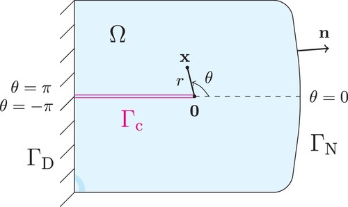We introduce the polar coordinates r>0 and $\theta \in (-\pi ,\pi )$ such that the upper and lower crack faces correspond to $\theta =\pm \pi$, respectively, as illustrated in Figure 1.

Figure 1. Example geometry of a planar sectorial domain ${\mathrm{\Omega }}_{\text{c}}$ with crack ${\mathrm{\Gamma }}_{\text{c}}$.

In the sectorial domain ${\mathrm{\Omega }}_{\text{c}}$, we look for unknown vector $\mathbf{u}=(u_r,u_{\theta })(r,\theta )$ and scalar $p(r,\theta )$ functions. They constitute the linearized strain $\mathit{\epsilon }(r,\theta )$ and the Cauchy stress $\mathit{\tau }(r,\theta )$ defined according to (2(2) $\begin{array}{r}\mathit{\tau }=2\mu \mathit{\epsilon }(\mathbf{u})-p\mathbf{I},\mathit{\epsilon }(\mathbf{u})=\frac{1}{2}(\mathrm{\nabla }\mathbf{u}+\mathrm{\nabla }{\mathbf{u}}^{\mathrm{\top }}),\end{array}$(2) ), which in the polar coordinates are represented by symmetric tensors in ${\mathbb{R}}_{\text{sym}}^{2\times 2}$ as (15) $\begin{array}{r}\mathit{\tau }=\left(\begin{array}{cc}{\tau }_{rr}& {\tau }_{r\theta }\\ {\tau }_{r\theta }& {\tau }_{\theta \theta }\end{array}\right)=\left(\begin{array}{cc}2\mu {\epsilon }_{rr}(\mathbf{u})-p& 2\mu {\epsilon }_{r\theta }(\mathbf{u})\\ 2\mu {\epsilon }_{r\theta }(\mathbf{u})& 2\mu {\epsilon }_{\theta \theta }(\mathbf{u})-p\end{array}\right),\mathit{\epsilon }(\mathbf{u})=\left(\begin{array}{cc}{\epsilon }_{rr}(\mathbf{u})& {\epsilon }_{r\theta }(\mathbf{u})\\ {\epsilon }_{r\theta }(\mathbf{u})& {\epsilon }_{\theta \theta }(\mathbf{u})\end{array}\right),\end{array}$(15) where the strain components are (16) $\begin{array}{r}{\epsilon }_{rr}(\mathbf{u})=u_{r,r},{\epsilon }_{r\theta }(\mathbf{u})=\frac{1}{2}(u_{\theta ,r}+\frac{1}{r}{u}_{r,\theta }-\frac{1}{r}{u}_{\theta }),{\epsilon }_{\theta \theta }(\mathbf{u})=\frac{1}{r}{u}_{\theta ,\theta }+\frac{1}{r}{u}_r,\end{array}$(16) using the convention for partial derivatives $(\cdot {)}_{,r}=\mathrm{\partial }(\cdot )/\mathrm{\partial }r$ and $(\cdot {)}_{,\theta }=\mathrm{\partial }(\cdot )/\mathrm{\partial }\theta$.

Applying the constitutive relations (15(15) $\begin{array}{r}\mathit{\tau }=\left(\begin{array}{cc}{\tau }_{rr}& {\tau }_{r\theta }\\ {\tau }_{r\theta }& {\tau }_{\theta \theta }\end{array}\right)=\left(\begin{array}{cc}2\mu {\epsilon }_{rr}(\mathbf{u})-p& 2\mu {\epsilon }_{r\theta }(\mathbf{u})\\ 2\mu {\epsilon }_{r\theta }(\mathbf{u})& 2\mu {\epsilon }_{\theta \theta }(\mathbf{u})-p\end{array}\right),\mathit{\epsilon }(\mathbf{u})=\left(\begin{array}{cc}{\epsilon }_{rr}(\mathbf{u})& {\epsilon }_{r\theta }(\mathbf{u})\\ {\epsilon }_{r\theta }(\mathbf{u})& {\epsilon }_{\theta \theta }(\mathbf{u})\end{array}\right),\end{array}$(15) ), the Stokes equation (1(1) $\begin{array}{r}-\mu \mathrm{\Delta }\mathbf{u}+\mathrm{\nabla }p=\mathbf{0},\text{div}\mathbf{u}=0,\end{array}$(1) ) turn into the equilibrium equations (17) $\begin{array}{r}-\text{div}\mathit{\tau }=\mathbf{0},\text{tr}\mathit{\epsilon }\mathbf{(}\mathbf{u}\mathbf{)}=0\text{in}{\mathrm{\Omega }}_{\text{c}},\end{array}$(17) where the identity for the trace $\text{tr}\mathit{\epsilon }(\mathbf{u})=\text{div}\mathbf{u}$ was used, such that in polar coordinates (18) $\begin{array}{r}{\tau }_{rr,r}+\frac{1}{r}{\tau }_{rr}+\frac{1}{r}{\tau }_{r\theta ,\theta }-\frac{1}{r}{\tau }_{\theta \theta }=0,{\tau }_{r\theta ,r}+\frac{2}{r}{\tau }_{r\theta }+\frac{1}{r}{\tau }_{\theta \theta ,\theta }=0,{\epsilon }_{rr}(\mathbf{u})+{\epsilon }_{\theta \theta }(\mathbf{u})=0.\end{array}$(18) At the outer boundary $\mathrm{\partial }\mathrm{\Omega }$, we endow (17(17) $\begin{array}{r}-\text{div}\mathit{\tau }=\mathbf{0},\text{tr}\mathit{\epsilon }\mathbf{(}\mathbf{u}\mathbf{)}=0\text{in}{\mathrm{\Omega }}_{\text{c}},\end{array}$(17) ) with the mixed, homogeneous Dirichlet–inhomogeneous Neumann boundary conditions (19) $\begin{array}{r}\mathbf{u}=\mathbf{0}\text{on }{\mathrm{\Gamma }}_{\text{D}},\mathit{\tau }\mathbf{n}=\mathbf{g}\text{on }{\mathrm{\Gamma }}_{\text{N}}\end{array}$(19) for a prescribed force $\mathbf{g}\in L^2({\mathrm{\Gamma }}_{\text{N}}{)}^2$, where $\mathit{\tau }\mathbf{n}$ stands for boundary traction.

Next we set admissible function spaces for the Stokes problems (17(17) $\begin{array}{r}-\text{div}\mathit{\tau }=\mathbf{0},\text{tr}\mathit{\epsilon }\mathbf{(}\mathbf{u}\mathbf{)}=0\text{in}{\mathrm{\Omega }}_{\text{c}},\end{array}$(17) ), (19(19) $\begin{array}{r}\mathbf{u}=\mathbf{0}\text{on }{\mathrm{\Gamma }}_{\text{D}},\mathit{\tau }\mathbf{n}=\mathbf{g}\text{on }{\mathrm{\Gamma }}_{\text{N}}\end{array}$(19) ) under boundary conditions (5(5) $\begin{array}{r}[[\mathbf{u}]]=\{\{\mathbf{u}\}\}=\mathbf{0},\end{array}$(5) )–(9(9) $\begin{array}{r}[[\mathit{\tau }-(\mathit{\tau }\cdot \mathbf{n})\mathbf{n}]]=\{\{\mathit{\tau }-(\mathit{\tau }\cdot \mathbf{n})\mathbf{n}\}\}=\mathbf{0},[[\mathit{\tau }\cdot \mathbf{n}]]=[[\mathbf{u}\cdot \mathbf{n}]]=0.\end{array}$(9) ) at the crack ${\mathrm{\Gamma }}_{\text{c}}$. Taking into account the no-slip condition in (19(19) $\begin{array}{r}\mathbf{u}=\mathbf{0}\text{on }{\mathrm{\Gamma }}_{\text{D}},\mathit{\tau }\mathbf{n}=\mathbf{g}\text{on }{\mathrm{\Gamma }}_{\text{N}}\end{array}$(19) ), we introduce the Sobolev space (20) $\begin{array}{r}V({\mathrm{\Omega }}_{\text{c}}):=\{\mathbf{u}\in H^1({\mathrm{\Omega }}_{\text{c}}{)}^2|\mathbf{u}=\mathbf{0}\text{on }{\mathrm{\Gamma }}_{\text{D}}\}.\end{array}$(20) Admissible at crack functions are restricted in a feasible set $K\subset V({\mathrm{\Omega }}_{\text{c}})$ meeting the Dirichlet case (5(5) $\begin{array}{r}[[\mathbf{u}]]=\{\{\mathbf{u}\}\}=\mathbf{0},\end{array}$(5) ) as (21) $\begin{array}{r}K=\{\mathbf{u}\in V({\mathrm{\Omega }}_{\text{c}})|[[\mathbf{u}]]=\{\{\mathbf{u}\}\}=\mathbf{0}\text{on }{\mathrm{\Gamma }}_{\text{c}}\},\end{array}$(21) the case of impermeability (6(6) $\begin{array}{r}[[\mathbf{u}\cdot \mathbf{n}]]=\{\{\mathbf{u}\cdot \mathbf{n}\}\}=0,[[\mathit{\tau }-(\mathit{\tau }\cdot \mathbf{n})\mathbf{n}]]=\{\{\mathit{\tau }-(\mathit{\tau }\cdot \mathbf{n})\mathbf{n}\}\}=\mathbf{0},\end{array}$(6) ) as (22) $\begin{array}{r}K=\{\mathbf{u}\in V({\mathrm{\Omega }}_{\text{c}})|[[u_{\theta }]]=\{\{u_{\theta }\}\}=0\text{on }{\mathrm{\Gamma }}_{\text{c}}\},\end{array}$(22) respectively in the Neumann case (7(7) $\begin{array}{r}[[\mathit{\tau }]]=\{\{\mathit{\tau }\}\}=\mathbf{0},\end{array}$(7) ) (23) $\begin{array}{r}K=V({\mathrm{\Omega }}_{\text{c}}),\end{array}$(23) the case of non-penetration (8(8) $\begin{array}{rl}[[\mathit{\tau }-(\mathit{\tau }\cdot \mathbf{n})\mathbf{n}]]& =\{\{\mathit{\tau }-(\mathit{\tau }\cdot \mathbf{n})\mathbf{n}\}\}=\mathbf{0},[[\mathit{\tau }\cdot \mathbf{n}]]=0,[[\mathbf{u}\cdot \mathbf{n}]]\ge 0,\\ \mathit{\tau }\cdot \mathbf{n}& \le 0,[[\mathbf{u}\cdot \mathbf{n}]](\mathit{\tau }\cdot \mathbf{n})=0,\end{array}$(8) ) implies (24) $\begin{array}{r}K=\{\mathbf{u}\in V({\mathrm{\Omega }}_{\text{c}})|[[u_{\theta }]]\le 0\text{on }{\mathrm{\Gamma }}_{\text{c}}\},\end{array}$(24) and the shear crack from (9(9) $\begin{array}{r}[[\mathit{\tau }-(\mathit{\tau }\cdot \mathbf{n})\mathbf{n}]]=\{\{\mathit{\tau }-(\mathit{\tau }\cdot \mathbf{n})\mathbf{n}\}\}=\mathbf{0},[[\mathit{\tau }\cdot \mathbf{n}]]=[[\mathbf{u}\cdot \mathbf{n}]]=0.\end{array}$(9) ) reads (25) $\begin{array}{r}K=\{\mathbf{u}\in V({\mathrm{\Omega }}_{\text{c}})|[[u_{\theta }]]=0\text{on }{\mathrm{\Gamma }}_{\text{c}}\}.\end{array}$(25) In all cases (21(21) $\begin{array}{r}K=\{\mathbf{u}\in V({\mathrm{\Omega }}_{\text{c}})|[[\mathbf{u}]]=\{\{\mathbf{u}\}\}=\mathbf{0}\text{on }{\mathrm{\Gamma }}_{\text{c}}\},\end{array}$(21) )–(25(25) $\begin{array}{r}K=\{\mathbf{u}\in V({\mathrm{\Omega }}_{\text{c}})|[[u_{\theta }]]=0\text{on }{\mathrm{\Gamma }}_{\text{c}}\}.\end{array}$(25) ), the topological set K yields a convex closed cone.

For stress tensors $\mathit{\tau }\in L^2({\mathrm{\Omega }}_{\text{c}};{\mathbb{R}}_{\text{sym}}^{2\times 2})$ such that $\text{div}\mathit{\tau }\in L^2({\mathrm{\Omega }}_{\text{c}}{)}^2$, the following Green's formula takes place using (18(18) $\begin{array}{r}{\tau }_{rr,r}+\frac{1}{r}{\tau }_{rr}+\frac{1}{r}{\tau }_{r\theta ,\theta }-\frac{1}{r}{\tau }_{\theta \theta }=0,{\tau }_{r\theta ,r}+\frac{2}{r}{\tau }_{r\theta }+\frac{1}{r}{\tau }_{\theta \theta ,\theta }=0,{\epsilon }_{rr}(\mathbf{u})+{\epsilon }_{\theta \theta }(\mathbf{u})=0.\end{array}$(18) ), and the notation from (3(3) $\begin{array}{r}[[\mathbf{u}]]:=\mathbf{u}{|}_{{\mathrm{\Gamma }}_{\text{c}}^{+}}-\mathbf{u}{|}_{{\mathrm{\Gamma }}_{\text{c}}^{-}},[[\mathit{\tau }]]:=\mathit{\tau }{|}_{{\mathrm{\Gamma }}_{\text{c}}^{+}}-\mathit{\tau }{|}_{{\mathrm{\Gamma }}_{\text{c}}^{-}},[[p]]:=p{|}_{{\mathrm{\Gamma }}_{\text{c}}^{+}}-p{|}_{{\mathrm{\Gamma }}_{\text{c}}^{-}},\end{array}$(3) ) and (4(4) $\begin{array}{r}\{\{\mathbf{u}\}\}:=\frac{1}{2}(\mathbf{u}{|}_{{\mathrm{\Gamma }}_{\text{c}}^{+}}+\mathbf{u}{|}_{{\mathrm{\Gamma }}_{\text{c}}^{-}}),\{\{\mathit{\tau }\}\}:=\frac{1}{2}(\mathit{\tau }{|}_{{\mathrm{\Gamma }}_{\text{c}}^{+}}+\mathit{\tau }{|}_{{\mathrm{\Gamma }}_{\text{c}}^{-}}),\{\{p\}\}:=\frac{1}{2}(p{|}_{{\mathrm{\Gamma }}_{\text{c}}^{+}}+p{|}_{{\mathrm{\Gamma }}_{\text{c}}^{-}}).\end{array}$(4) ): (26) $\begin{array}{rl}& -{\int }_{{\mathrm{\Omega }}_{\text{c}}}([(r{\tau }_{rr}{)}_{,r}+{\tau }_{r\theta ,\theta }-{\tau }_{\theta \theta }]v_r+[(r{\tau }_{r\theta }{)}_{,r}+{\tau }_{\theta \theta ,\theta }+{\tau }_{r\theta }]v_{\theta })drd\theta \\ & ={\int }_{{\mathrm{\Omega }}_{\text{c}}}({\tau }_{rr}{\epsilon }_{rr}(\mathbf{v})+2{\tau }_{r\theta }{\epsilon }_{r\theta }(\mathbf{v})+{\tau }_{\theta \theta }{\epsilon }_{\theta \theta }(\mathbf{v}))rdrd\theta \\ & -{\int }_{{\mathrm{\Gamma }}_{\text{N}}}\mathit{\tau }\mathbf{n}\cdot \mathbf{v}dS+{\int }_{{\mathrm{\Gamma }}_{\text{c}}}([[{\tau }_{r\theta }]]\{\{{\mathbf{v}}_r\}\}+\{\{{\tau }_{r\theta }\}\}[[{\mathbf{v}}_r]]+[[{\tau }_{\theta \theta }]]\{\{{\mathbf{v}}_{\theta }\}\}+\{\{{\tau }_{\theta \theta }\}\}[[{\mathbf{v}}_{\theta }]])rdr\end{array}$(26) for smooth functions $\mathbf{v}=(v_r,v_{\theta })$ such that $\mathbf{v}=\mathbf{0}$ on ${\mathrm{\Gamma }}_{\text{D}}$, and the strain operator $\mathit{\epsilon }(\mathbf{v})$ defined according to (16(16) $\begin{array}{r}{\epsilon }_{rr}(\mathbf{u})=u_{r,r},{\epsilon }_{r\theta }(\mathbf{u})=\frac{1}{2}(u_{\theta ,r}+\frac{1}{r}{u}_{r,\theta }-\frac{1}{r}{u}_{\theta }),{\epsilon }_{\theta \theta }(\mathbf{u})=\frac{1}{r}{u}_{\theta ,\theta }+\frac{1}{r}{u}_r,\end{array}$(16) ). After integration of Equation (17(17) $\begin{array}{r}-\text{div}\mathit{\tau }=\mathbf{0},\text{tr}\mathit{\epsilon }\mathbf{(}\mathbf{u}\mathbf{)}=0\text{in}{\mathrm{\Omega }}_{\text{c}},\end{array}$(17) ) with the help of constitutive relations (15(15) $\begin{array}{r}\mathit{\tau }=\left(\begin{array}{cc}{\tau }_{rr}& {\tau }_{r\theta }\\ {\tau }_{r\theta }& {\tau }_{\theta \theta }\end{array}\right)=\left(\begin{array}{cc}2\mu {\epsilon }_{rr}(\mathbf{u})-p& 2\mu {\epsilon }_{r\theta }(\mathbf{u})\\ 2\mu {\epsilon }_{r\theta }(\mathbf{u})& 2\mu {\epsilon }_{\theta \theta }(\mathbf{u})-p\end{array}\right),\mathit{\epsilon }(\mathbf{u})=\left(\begin{array}{cc}{\epsilon }_{rr}(\mathbf{u})& {\epsilon }_{r\theta }(\mathbf{u})\\ {\epsilon }_{r\theta }(\mathbf{u})& {\epsilon }_{\theta \theta }(\mathbf{u})\end{array}\right),\end{array}$(15) ), boundary conditions (19(19) $\begin{array}{r}\mathbf{u}=\mathbf{0}\text{on }{\mathrm{\Gamma }}_{\text{D}},\mathit{\tau }\mathbf{n}=\mathbf{g}\text{on }{\mathrm{\Gamma }}_{\text{N}}\end{array}$(19) ) and Green's formula (26(26) $\begin{array}{rl}& -{\int }_{{\mathrm{\Omega }}_{\text{c}}}([(r{\tau }_{rr}{)}_{,r}+{\tau }_{r\theta ,\theta }-{\tau }_{\theta \theta }]v_r+[(r{\tau }_{r\theta }{)}_{,r}+{\tau }_{\theta \theta ,\theta }+{\tau }_{r\theta }]v_{\theta })drd\theta \\ & ={\int }_{{\mathrm{\Omega }}_{\text{c}}}({\tau }_{rr}{\epsilon }_{rr}(\mathbf{v})+2{\tau }_{r\theta }{\epsilon }_{r\theta }(\mathbf{v})+{\tau }_{\theta \theta }{\epsilon }_{\theta \theta }(\mathbf{v}))rdrd\theta \\ & -{\int }_{{\mathrm{\Gamma }}_{\text{N}}}\mathit{\tau }\mathbf{n}\cdot \mathbf{v}dS+{\int }_{{\mathrm{\Gamma }}_{\text{c}}}([[{\tau }_{r\theta }]]\{\{{\mathbf{v}}_r\}\}+\{\{{\tau }_{r\theta }\}\}[[{\mathbf{v}}_r]]+[[{\tau }_{\theta \theta }]]\{\{{\mathbf{v}}_{\theta }\}\}+\{\{{\tau }_{\theta \theta }\}\}[[{\mathbf{v}}_{\theta }]])rdr\end{array}$(26) ), we arrive at the variational inequality: find $(\mathbf{u},p)\in K\times L^2({\mathrm{\Omega }}_{\text{c}})$ satisfying (27) $\begin{array}{rl}& {\int }_{{\mathrm{\Omega }}_{\text{c}}}((2\mu {\epsilon }_{rr}(\mathbf{u})-p){\epsilon }_{rr}(\mathbf{v}-\mathbf{u})+4\mu {\epsilon }_{r\theta }(\mathbf{u}){\epsilon }_{r\theta }(\mathbf{v}-\mathbf{u})\\ & +(2\mu {\epsilon }_{\theta \theta }(\mathbf{u})-p){\epsilon }_{\theta \theta }(\mathbf{v}-\mathbf{u}))rdrd\theta \ge {\int }_{{\mathrm{\Gamma }}_{\text{N}}}\mathbf{g}\cdot (\mathbf{v}-\mathbf{u})dS\end{array}$(27) for all test functions $\mathbf{v}\in K$. This system is completed with the weak form of incompressibility as (28) $\begin{array}{r}{\int }_{{\mathrm{\Omega }}_{\text{c}}}({\epsilon }_{rr}(\mathbf{u})+{\epsilon }_{\theta \theta }(\mathbf{u}))qrdrd\theta =0\end{array}$(28) for all test functions $q\in L^2({\mathrm{\Omega }}_{\text{c}})$. Conversely, for the smooth solution $(\mathbf{u},p)\in H^2({\mathrm{\Omega }}_{\text{c}}{)}^2\times H^1({\mathrm{\Omega }}_{\text{c}})$, the boundary conditions on the stress in (5(5) $\begin{array}{r}[[\mathbf{u}]]=\{\{\mathbf{u}\}\}=\mathbf{0},\end{array}$(5) )–(9(9) $\begin{array}{r}[[\mathit{\tau }-(\mathit{\tau }\cdot \mathbf{n})\mathbf{n}]]=\{\{\mathit{\tau }-(\mathit{\tau }\cdot \mathbf{n})\mathbf{n}\}\}=\mathbf{0},[[\mathit{\tau }\cdot \mathbf{n}]]=[[\mathbf{u}\cdot \mathbf{n}]]=0.\end{array}$(9) ) follow from the variational inequality (27(27) $\begin{array}{rl}& {\int }_{{\mathrm{\Omega }}_{\text{c}}}((2\mu {\epsilon }_{rr}(\mathbf{u})-p){\epsilon }_{rr}(\mathbf{v}-\mathbf{u})+4\mu {\epsilon }_{r\theta }(\mathbf{u}){\epsilon }_{r\theta }(\mathbf{v}-\mathbf{u})\\ & +(2\mu {\epsilon }_{\theta \theta }(\mathbf{u})-p){\epsilon }_{\theta \theta }(\mathbf{v}-\mathbf{u}))rdrd\theta \ge {\int }_{{\mathrm{\Gamma }}_{\text{N}}}\mathbf{g}\cdot (\mathbf{v}-\mathbf{u})dS\end{array}$(27) ) after applying Green's formula (26(26) $\begin{array}{rl}& -{\int }_{{\mathrm{\Omega }}_{\text{c}}}([(r{\tau }_{rr}{)}_{,r}+{\tau }_{r\theta ,\theta }-{\tau }_{\theta \theta }]v_r+[(r{\tau }_{r\theta }{)}_{,r}+{\tau }_{\theta \theta ,\theta }+{\tau }_{r\theta }]v_{\theta })drd\theta \\ & ={\int }_{{\mathrm{\Omega }}_{\text{c}}}({\tau }_{rr}{\epsilon }_{rr}(\mathbf{v})+2{\tau }_{r\theta }{\epsilon }_{r\theta }(\mathbf{v})+{\tau }_{\theta \theta }{\epsilon }_{\theta \theta }(\mathbf{v}))rdrd\theta \\ & -{\int }_{{\mathrm{\Gamma }}_{\text{N}}}\mathit{\tau }\mathbf{n}\cdot \mathbf{v}dS+{\int }_{{\mathrm{\Gamma }}_{\text{c}}}([[{\tau }_{r\theta }]]\{\{{\mathbf{v}}_r\}\}+\{\{{\tau }_{r\theta }\}\}[[{\mathbf{v}}_r]]+[[{\tau }_{\theta \theta }]]\{\{{\mathbf{v}}_{\theta }\}\}+\{\{{\tau }_{\theta \theta }\}\}[[{\mathbf{v}}_{\theta }]])rdr\end{array}$(26) ).

Proposition 2.1

(Well-posedness of the weak Stokes problems). Let $K\subset V({\mathrm{\Omega }}_{\text{c}})$ be a generic feasible set, which is convex and closed (e.g. (21(21) $\begin{array}{r}K=\{\mathbf{u}\in V({\mathrm{\Omega }}_{\text{c}})|[[\mathbf{u}]]=\{\{\mathbf{u}\}\}=\mathbf{0}\text{on }{\mathrm{\Gamma }}_{\text{c}}\},\end{array}$(21) )–(25(25) $\begin{array}{r}K=\{\mathbf{u}\in V({\mathrm{\Omega }}_{\text{c}})|[[u_{\theta }]]=0\text{on }{\mathrm{\Gamma }}_{\text{c}}\}.\end{array}$(25) )). Then there exists a pair $(\mathbf{u},p)\in K\times L^2({\mathrm{\Omega }}_{\text{c}})$, the stress and strain $\mathit{\tau },\mathit{\epsilon }\in L^2({\mathrm{\Omega }}_{\text{c}};{\mathbb{R}}_{\text{sym}}^{2\times 2})$ determined from (15(15) $\begin{array}{r}\mathit{\tau }=\left(\begin{array}{cc}{\tau }_{rr}& {\tau }_{r\theta }\\ {\tau }_{r\theta }& {\tau }_{\theta \theta }\end{array}\right)=\left(\begin{array}{cc}2\mu {\epsilon }_{rr}(\mathbf{u})-p& 2\mu {\epsilon }_{r\theta }(\mathbf{u})\\ 2\mu {\epsilon }_{r\theta }(\mathbf{u})& 2\mu {\epsilon }_{\theta \theta }(\mathbf{u})-p\end{array}\right),\mathit{\epsilon }(\mathbf{u})=\left(\begin{array}{cc}{\epsilon }_{rr}(\mathbf{u})& {\epsilon }_{r\theta }(\mathbf{u})\\ {\epsilon }_{r\theta }(\mathbf{u})& {\epsilon }_{\theta \theta }(\mathbf{u})\end{array}\right),\end{array}$(15) ) and (16(16) $\begin{array}{r}{\epsilon }_{rr}(\mathbf{u})=u_{r,r},{\epsilon }_{r\theta }(\mathbf{u})=\frac{1}{2}(u_{\theta ,r}+\frac{1}{r}{u}_{r,\theta }-\frac{1}{r}{u}_{\theta }),{\epsilon }_{\theta \theta }(\mathbf{u})=\frac{1}{r}{u}_{\theta ,\theta }+\frac{1}{r}{u}_r,\end{array}$(16) ), which solve uniquely the variational relations (27(27) $\begin{array}{rl}& {\int }_{{\mathrm{\Omega }}_{\text{c}}}((2\mu {\epsilon }_{rr}(\mathbf{u})-p){\epsilon }_{rr}(\mathbf{v}-\mathbf{u})+4\mu {\epsilon }_{r\theta }(\mathbf{u}){\epsilon }_{r\theta }(\mathbf{v}-\mathbf{u})\\ & +(2\mu {\epsilon }_{\theta \theta }(\mathbf{u})-p){\epsilon }_{\theta \theta }(\mathbf{v}-\mathbf{u}))rdrd\theta \ge {\int }_{{\mathrm{\Gamma }}_{\text{N}}}\mathbf{g}\cdot (\mathbf{v}-\mathbf{u})dS\end{array}$(27) ) and (28(28) $\begin{array}{r}{\int }_{{\mathrm{\Omega }}_{\text{c}}}({\epsilon }_{rr}(\mathbf{u})+{\epsilon }_{\theta \theta }(\mathbf{u}))qrdrd\theta =0\end{array}$(28) ).

Proof.

In the proof we recall the well-known facts from the theory of mixed variational problems for the Stokes equations (see, e.g. Ref. [5]). The weak formulation (27(27) $\begin{array}{rl}& {\int }_{{\mathrm{\Omega }}_{\text{c}}}((2\mu {\epsilon }_{rr}(\mathbf{u})-p){\epsilon }_{rr}(\mathbf{v}-\mathbf{u})+4\mu {\epsilon }_{r\theta }(\mathbf{u}){\epsilon }_{r\theta }(\mathbf{v}-\mathbf{u})\\ & +(2\mu {\epsilon }_{\theta \theta }(\mathbf{u})-p){\epsilon }_{\theta \theta }(\mathbf{v}-\mathbf{u}))rdrd\theta \ge {\int }_{{\mathrm{\Gamma }}_{\text{N}}}\mathbf{g}\cdot (\mathbf{v}-\mathbf{u})dS\end{array}$(27) ) and (28(28) $\begin{array}{r}{\int }_{{\mathrm{\Omega }}_{\text{c}}}({\epsilon }_{rr}(\mathbf{u})+{\epsilon }_{\theta \theta }(\mathbf{u}))qrdrd\theta =0\end{array}$(28) ) gives rise to the Lagrangian function $\mathcal{L}:V({\mathrm{\Omega }}_{\text{c}})\times L^2({\mathrm{\Omega }}_{\text{c}})\mapsto \mathbb{R}$ (the free energy), which is well-defined by (29) $\begin{array}{rl}\mathcal{L}(\mathbf{u},p)& ={\int }_{{\mathrm{\Omega }}_{\text{c}}}((2\mu {\epsilon }_{rr}(\mathbf{u})-p){\epsilon }_{rr}(\mathbf{u})+4\mu {\epsilon }_{r\theta }(\mathbf{u}){\epsilon }_{r\theta }(\mathbf{u})\\ & +(2\mu {\epsilon }_{\theta \theta }(\mathbf{u})-p){\epsilon }_{\theta \theta }(\mathbf{u}))rdrd\theta -{\int }_{{\mathrm{\Gamma }}_{\text{N}}}\mathbf{g}\cdot \mathbf{u}dS.\end{array}$(29) The mapping $[\mathbf{u}\mapsto \mathcal{L}(\mathbf{u},p)]$ in (29(29) $\begin{array}{rl}\mathcal{L}(\mathbf{u},p)& ={\int }_{{\mathrm{\Omega }}_{\text{c}}}((2\mu {\epsilon }_{rr}(\mathbf{u})-p){\epsilon }_{rr}(\mathbf{u})+4\mu {\epsilon }_{r\theta }(\mathbf{u}){\epsilon }_{r\theta }(\mathbf{u})\\ & +(2\mu {\epsilon }_{\theta \theta }(\mathbf{u})-p){\epsilon }_{\theta \theta }(\mathbf{u}))rdrd\theta -{\int }_{{\mathrm{\Gamma }}_{\text{N}}}\mathbf{g}\cdot \mathbf{u}dS.\end{array}$(29) ) is quadratic, convex and coercive due to Poincare inequality provided by the Dirichlet condition in (20(20) $\begin{array}{r}V({\mathrm{\Omega }}_{\text{c}}):=\{\mathbf{u}\in H^1({\mathrm{\Omega }}_{\text{c}}{)}^2|\mathbf{u}=\mathbf{0}\text{on }{\mathrm{\Gamma }}_{\text{D}}\}.\end{array}$(20) ) such that (30) $\begin{array}{rl}& \mathcal{L}(\mathbf{u},p)\ge c_{\text{P}}\Vert \mathbf{u}{\Vert }_{H^1({\mathrm{\Omega }}_{\text{c}}{)}^2}^2\\ & -c(\Vert p{\Vert }_{L^2({\mathrm{\Omega }}_{\text{c}})}+\Vert \mathbf{g}{\Vert }_{L^2({\mathrm{\Gamma }}_{\text{N}}{)}^2})\Vert \mathbf{u}{\Vert }_{H^1({\mathrm{\Omega }}_{\text{c}}{)}^2}\to +\mathrm{\infty }\text{as}\Vert \mathbf{u}{\Vert }_{H^1({\mathrm{\Omega }}_{\text{c}}{)}^2}\to \mathrm{\infty }.\end{array}$(30) The operator $[\mathbf{u}\mapsto \text{tr}\mathit{\epsilon }]:V({\mathrm{\Omega }}_{\text{c}})\mapsto L^2({\mathrm{\Omega }}_{\text{c}})$ in (18(18) $\begin{array}{r}{\tau }_{rr,r}+\frac{1}{r}{\tau }_{rr}+\frac{1}{r}{\tau }_{r\theta ,\theta }-\frac{1}{r}{\tau }_{\theta \theta }=0,{\tau }_{r\theta ,r}+\frac{2}{r}{\tau }_{r\theta }+\frac{1}{r}{\tau }_{\theta \theta ,\theta }=0,{\epsilon }_{rr}(\mathbf{u})+{\epsilon }_{\theta \theta }(\mathbf{u})=0.\end{array}$(18) ) is surjective. Therefore, the inf-sup condition (see Ref. [1]) for the linear mapping $[p\mapsto \mathcal{L}(\mathbf{u},p)]$ in (29(29) $\begin{array}{rl}\mathcal{L}(\mathbf{u},p)& ={\int }_{{\mathrm{\Omega }}_{\text{c}}}((2\mu {\epsilon }_{rr}(\mathbf{u})-p){\epsilon }_{rr}(\mathbf{u})+4\mu {\epsilon }_{r\theta }(\mathbf{u}){\epsilon }_{r\theta }(\mathbf{u})\\ & +(2\mu {\epsilon }_{\theta \theta }(\mathbf{u})-p){\epsilon }_{\theta \theta }(\mathbf{u}))rdrd\theta -{\int }_{{\mathrm{\Gamma }}_{\text{N}}}\mathbf{g}\cdot \mathbf{u}dS.\end{array}$(29) ) follows directly from the definition of dual norm in $L^2({\mathrm{\Omega }}_{\text{c}})$: (31) $\begin{array}{r}\underset{0\ne \mathbf{u}\in H^1({\mathrm{\Omega }}_{\text{c}}{)}^2}{sup}\frac{1}{\Vert \mathbf{u}{\Vert }_{H^1({\mathrm{\Omega }}_{\text{c}}{)}^2}}{\int }_{{\mathrm{\Omega }}_{\text{c}}}({\epsilon }_{rr}(\mathbf{u})+{\epsilon }_{\theta \theta }(\mathbf{u}))prdrd\theta \ge c_{\text{LBB}}\Vert p{\Vert }_{L^2({\mathrm{\Omega }}_{\text{c}})},c_{\text{LBB}}>0.\end{array}$(31) As the consequence of Ladyzhenskaya–Babuška–Brezzi–Nečas minimax theorem, there exists a unique saddle point $(\mathbf{u},p)\in K\times L^2({\mathrm{\Omega }}_{\text{c}})$ such that (32) $\begin{array}{r}\mathcal{L}(\mathbf{u},q)\le \mathcal{L}(\mathbf{u},p)\le \mathcal{L}(\mathbf{v},p)\end{array}$(32) for all test functions $(\mathbf{v},q)\in K\times L^2({\mathrm{\Omega }}_{\text{c}})$. After differentiation with respect to $\mathbf{u}$ and p, the optimality conditions for (32(32) $\begin{array}{r}\mathcal{L}(\mathbf{u},q)\le \mathcal{L}(\mathbf{u},p)\le \mathcal{L}(\mathbf{v},p)\end{array}$(32) ) lead to the variational inequality (27(27) $\begin{array}{rl}& {\int }_{{\mathrm{\Omega }}_{\text{c}}}((2\mu {\epsilon }_{rr}(\mathbf{u})-p){\epsilon }_{rr}(\mathbf{v}-\mathbf{u})+4\mu {\epsilon }_{r\theta }(\mathbf{u}){\epsilon }_{r\theta }(\mathbf{v}-\mathbf{u})\\ & +(2\mu {\epsilon }_{\theta \theta }(\mathbf{u})-p){\epsilon }_{\theta \theta }(\mathbf{v}-\mathbf{u}))rdrd\theta \ge {\int }_{{\mathrm{\Gamma }}_{\text{N}}}\mathbf{g}\cdot (\mathbf{v}-\mathbf{u})dS\end{array}$(27) ) and Equation (28(28) $\begin{array}{r}{\int }_{{\mathrm{\Omega }}_{\text{c}}}({\epsilon }_{rr}(\mathbf{u})+{\epsilon }_{\theta \theta }(\mathbf{u}))qrdrd\theta =0\end{array}$(28) ). The proof is completed.

Evidently, the assertion of Proposition 2.1 holds for much more general geometries than assumed at the beginning of this section. In the subsequent sections, we use these geometric assumptions for construction of a semi-analytic solution for the variational Stokes problems locally in a neighbourhood of the crack tip.

3. Power series solution in the general form

To write the equilibrium equations in terms of $\mathbf{u}$, we substitute the stress $\mathit{\tau }$ from (15(15) $\begin{array}{r}\mathit{\tau }=\left(\begin{array}{cc}{\tau }_{rr}& {\tau }_{r\theta }\\ {\tau }_{r\theta }& {\tau }_{\theta \theta }\end{array}\right)=\left(\begin{array}{cc}2\mu {\epsilon }_{rr}(\mathbf{u})-p& 2\mu {\epsilon }_{r\theta }(\mathbf{u})\\ 2\mu {\epsilon }_{r\theta }(\mathbf{u})& 2\mu {\epsilon }_{\theta \theta }(\mathbf{u})-p\end{array}\right),\mathit{\epsilon }(\mathbf{u})=\left(\begin{array}{cc}{\epsilon }_{rr}(\mathbf{u})& {\epsilon }_{r\theta }(\mathbf{u})\\ {\epsilon }_{r\theta }(\mathbf{u})& {\epsilon }_{\theta \theta }(\mathbf{u})\end{array}\right),\end{array}$(15) ) and strain $\mathit{\epsilon }(\mathbf{u})$ from (16(16) $\begin{array}{r}{\epsilon }_{rr}(\mathbf{u})=u_{r,r},{\epsilon }_{r\theta }(\mathbf{u})=\frac{1}{2}(u_{\theta ,r}+\frac{1}{r}{u}_{r,\theta }-\frac{1}{r}{u}_{\theta }),{\epsilon }_{\theta \theta }(\mathbf{u})=\frac{1}{r}{u}_{\theta ,\theta }+\frac{1}{r}{u}_r,\end{array}$(16) ) into the first two equations in (18(18) $\begin{array}{r}{\tau }_{rr,r}+\frac{1}{r}{\tau }_{rr}+\frac{1}{r}{\tau }_{r\theta ,\theta }-\frac{1}{r}{\tau }_{\theta \theta }=0,{\tau }_{r\theta ,r}+\frac{2}{r}{\tau }_{r\theta }+\frac{1}{r}{\tau }_{\theta \theta ,\theta }=0,{\epsilon }_{rr}(\mathbf{u})+{\epsilon }_{\theta \theta }(\mathbf{u})=0.\end{array}$(18) ), and use the incompressibility ${\epsilon }_{rr}(\mathbf{u})+{\epsilon }_{\theta \theta }(\mathbf{u})=0$ such that $\begin{array}{rl}& 2\mu ({\epsilon }_{\theta \theta ,r}(\mathbf{u})-\frac{1}{r}{\epsilon }_{rr}(\mathbf{u})-\frac{1}{r}{\epsilon }_{r\theta ,\theta }(\mathbf{u})+\frac{1}{r}{\epsilon }_{\theta \theta }(\mathbf{u}))+p_{,r}=0,\\ & 2\mu ({\epsilon }_{r\theta ,r}(\mathbf{u})+\frac{2}{r}{\epsilon }_{r\theta }(\mathbf{u})-\frac{1}{r}{\epsilon }_{rr,\theta }(\mathbf{u}))-\frac{1}{r}{p}_{,\theta }=0.\end{array}$Due to the symmetry of mixed derivatives, differentiating (16(16) $\begin{array}{r}{\epsilon }_{rr}(\mathbf{u})=u_{r,r},{\epsilon }_{r\theta }(\mathbf{u})=\frac{1}{2}(u_{\theta ,r}+\frac{1}{r}{u}_{r,\theta }-\frac{1}{r}{u}_{\theta }),{\epsilon }_{\theta \theta }(\mathbf{u})=\frac{1}{r}{u}_{\theta ,\theta }+\frac{1}{r}{u}_r,\end{array}$(16) ) yields two compatibility conditions $\begin{array}{rl}{\epsilon }_{\theta \theta ,r}(\mathbf{u})& =\frac{1}{r}{\epsilon }_{rr}(\mathbf{u})+\frac{2}{r}{\epsilon }_{r\theta ,\theta }(\mathbf{u})-\frac{1}{r}{\epsilon }_{\theta \theta }(\mathbf{u})-\frac{1}{r^2}{u}_{r,\theta \theta }+\frac{1}{r^2}{u}_{\theta ,\theta },\\ \frac{1}{r}{\epsilon }_{rr,\theta }(\mathbf{u})& =2{\epsilon }_{r\theta ,r}(\mathbf{u})+\frac{2}{r}{\epsilon }_{r\theta }(\mathbf{u})-u_{\theta ,rr}.\end{array}$Inserting these conditions justifies the equilibrium equations as (33) $\begin{array}{r}\frac{\mu }{r}\eta (\mathbf{u}{)}_{,\theta }+p_{,r}=0,\mu \eta (\mathbf{u}{)}_{,r}-\frac{1}{r}{p}_{,\theta }=0,\text{where }\eta (\mathbf{u}):=u_{\theta ,r}+\frac{1}{r}{u}_{\theta }-\frac{1}{r}{u}_{r,\theta }.\end{array}$(33) In its turn, the incompressibility condition in terms of $\mathbf{u}$ reads (34) $\begin{array}{r}{u}_{r,r}+\frac{1}{r}{u}_r+\frac{1}{r}{u}_{\theta ,\theta }=0.\end{array}$(34) We look for the solution of Stokes Equations (33(33) $\begin{array}{r}\frac{\mu }{r}\eta (\mathbf{u}{)}_{,\theta }+p_{,r}=0,\mu \eta (\mathbf{u}{)}_{,r}-\frac{1}{r}{p}_{,\theta }=0,\text{where }\eta (\mathbf{u}):=u_{\theta ,r}+\frac{1}{r}{u}_{\theta }-\frac{1}{r}{u}_{r,\theta }.\end{array}$(33) ) and (34(34) $\begin{array}{r}{u}_{r,r}+\frac{1}{r}{u}_r+\frac{1}{r}{u}_{\theta ,\theta }=0.\end{array}$(34) ) by the Fourier series (10(10) $\begin{array}{rl}\mathbf{u}(r,\theta )& =\sum _{\gamma \in \mathbb{R}}{r}^{\gamma }\sum _{m=0}^{M(\gamma )}\frac{(\ln r{)}^{M(\gamma )-m}}{(M(\gamma )-m)!}{\mathbf{\Psi }}^m(\gamma ,\theta ),\\ p(r,\theta )& =\sum _{\gamma \in \mathbb{R}}{r}^{\gamma -1}\sum _{m=0}^{M(\gamma )}\frac{(\ln r{)}^{M(\gamma )-m}}{(M(\gamma )-m)!}{\mathrm{\Phi }}^m(\gamma ,\theta ),\end{array}$(10) ) with respect to powers γ (see Ref. [22]). For every fixed $\gamma \in \mathbb{R}$, we consider the asymptotic terms (35) $\begin{array}{rl}{\mathbf{u}}^{\gamma }(r,\theta )& =r^{\gamma }\sum _{m=0}^M\frac{(\ln r{)}^{M-m}}{(M-m)!}{\mathbf{\Psi }}^m(\gamma ,\theta ),\\ p^{\gamma }(r,\theta )& =r^{\gamma -1}\sum _{m=0}^M\frac{(\ln r{)}^{M-m}}{(M-m)!}{\mathrm{\Phi }}^m(\gamma ,\theta )(M\ge 0)\end{array}$(35) with unknown angular vector ${\mathbf{\Psi }}^0,\dots ,{\mathbf{\Psi }}^M$ and scalar ${\mathrm{\Phi }}^0,\dots ,{\mathrm{\Phi }}^M$ functions. Here, the $\gamma -1$-power for the pressure is due to compatibility of the terms in the stress $\mathit{\tau }$ entering the constitutive equation (15(15) $\begin{array}{r}\mathit{\tau }=\left(\begin{array}{cc}{\tau }_{rr}& {\tau }_{r\theta }\\ {\tau }_{r\theta }& {\tau }_{\theta \theta }\end{array}\right)=\left(\begin{array}{cc}2\mu {\epsilon }_{rr}(\mathbf{u})-p& 2\mu {\epsilon }_{r\theta }(\mathbf{u})\\ 2\mu {\epsilon }_{r\theta }(\mathbf{u})& 2\mu {\epsilon }_{\theta \theta }(\mathbf{u})-p\end{array}\right),\mathit{\epsilon }(\mathbf{u})=\left(\begin{array}{cc}{\epsilon }_{rr}(\mathbf{u})& {\epsilon }_{r\theta }(\mathbf{u})\\ {\epsilon }_{r\theta }(\mathbf{u})& {\epsilon }_{\theta \theta }(\mathbf{u})\end{array}\right),\end{array}$(15) ). Our task needs few auxiliary lemmas.

Lemma 3.1

(Recurrence equations for angular functions). If the angular functions satisfy the following recurrence equations: (36) $\begin{array}{rl}& (\gamma +1){\mathrm{\Psi }}_r^0+{\mathrm{\Psi }}_{\theta ,\theta }^0=0,(\gamma +1){\mathrm{\Psi }}_r^m+{\mathrm{\Psi }}_{\theta ,\theta }^m+{\mathrm{\Psi }}_r^{m-1}=0\text{for }m=1,\dots ,M,\end{array}$(36) (37) $\begin{array}{rl}& \mu [(\gamma +1){\mathrm{\Psi }}_{\theta ,\theta }^0-{\mathrm{\Psi }}_{r,\theta \theta }^0]+(\gamma -1){\mathrm{\Phi }}^0=0,\\ & \mu [(\gamma +1){\mathrm{\Psi }}_{\theta ,\theta }^m-{\mathrm{\Psi }}_{r,\theta \theta }^m+{\mathrm{\Psi }}_{\theta ,\theta }^{m-1}]+(\gamma -1){\mathrm{\Phi }}^m+{\mathrm{\Phi }}^{m-1}=0\text{for }m=1,\dots ,M,\end{array}$(37) (38) $\begin{array}{rl}& \mu (\gamma -1)[(\gamma +1){\mathrm{\Psi }}_{\theta }^0-{\mathrm{\Psi }}_{r,\theta }^0]-{\mathrm{\Phi }}_{,\theta }^0=0,\\ & \mu [({\gamma }^2-1){\mathrm{\Psi }}_{\theta }^1-(\gamma -1){\mathrm{\Psi }}_{r,\theta }^1+2\gamma {\mathrm{\Psi }}_{\theta }^0-{\mathrm{\Psi }}_{r,\theta }^0]-{\mathrm{\Phi }}_{,\theta }^1=0,\\ & \mu [({\gamma }^2-1){\mathrm{\Psi }}_{\theta }^m-(\gamma -1){\mathrm{\Psi }}_{r,\theta }^m+2\gamma {\mathrm{\Psi }}_{\theta }^{m-1}-{\mathrm{\Psi }}_{r,\theta }^{m-1}+{\mathrm{\Psi }}_{\theta }^{m-2}]\\ & -{\mathrm{\Phi }}_{,\theta }^m=0\text{for }m=2,\dots ,M,\end{array}$(38) then ansatz (35(35) $\begin{array}{rl}{\mathbf{u}}^{\gamma }(r,\theta )& =r^{\gamma }\sum _{m=0}^M\frac{(\ln r{)}^{M-m}}{(M-m)!}{\mathbf{\Psi }}^m(\gamma ,\theta ),\\ p^{\gamma }(r,\theta )& =r^{\gamma -1}\sum _{m=0}^M\frac{(\ln r{)}^{M-m}}{(M-m)!}{\mathrm{\Phi }}^m(\gamma ,\theta )(M\ge 0)\end{array}$(35) ) fulfils the Stokes equations (33(33) $\begin{array}{r}\frac{\mu }{r}\eta (\mathbf{u}{)}_{,\theta }+p_{,r}=0,\mu \eta (\mathbf{u}{)}_{,r}-\frac{1}{r}{p}_{,\theta }=0,\text{where }\eta (\mathbf{u}):=u_{\theta ,r}+\frac{1}{r}{u}_{\theta }-\frac{1}{r}{u}_{r,\theta }.\end{array}$(33) ) and (34(34) $\begin{array}{r}{u}_{r,r}+\frac{1}{r}{u}_r+\frac{1}{r}{u}_{\theta ,\theta }=0.\end{array}$(34) ).

Proof.

For differentiation of the power series with respect to r, we exploit the following calculus: (39) $\begin{array}{rl}{\mathbf{u}}_{,r}^{\gamma }& =r^{\gamma -1}(\gamma \sum _{m=0}^M\frac{(\ln r{)}^{M-m}}{(M-m)!}{\mathbf{\Psi }}^m+\sum _{m=0}^{M-1}\frac{(\ln r{)}^{M-m-1}}{(M-m-1)!}{\mathbf{\Psi }}^m)\\ & =r^{\gamma -1}(\frac{(\ln r{)}^M}{M!}\gamma {\mathbf{\Psi }}^0+\sum _{m=1}^M\frac{(\ln r{)}^{M-m}}{(M-m)!}(\gamma {\mathbf{\Psi }}^m+{\mathbf{\Psi }}^{m-1})),\end{array}$(39) where shifting of the summation index was used. Inserting ansatz (35(35) $\begin{array}{rl}{\mathbf{u}}^{\gamma }(r,\theta )& =r^{\gamma }\sum _{m=0}^M\frac{(\ln r{)}^{M-m}}{(M-m)!}{\mathbf{\Psi }}^m(\gamma ,\theta ),\\ p^{\gamma }(r,\theta )& =r^{\gamma -1}\sum _{m=0}^M\frac{(\ln r{)}^{M-m}}{(M-m)!}{\mathrm{\Phi }}^m(\gamma ,\theta )(M\ge 0)\end{array}$(35) ) into the incompressibility equation (34(34) $\begin{array}{r}{u}_{r,r}+\frac{1}{r}{u}_r+\frac{1}{r}{u}_{\theta ,\theta }=0.\end{array}$(34) ), after the differentiation of ${\mathbf{u}}^{\gamma }$ with respect to θ and r as in (39(39) $\begin{array}{rl}{\mathbf{u}}_{,r}^{\gamma }& =r^{\gamma -1}(\gamma \sum _{m=0}^M\frac{(\ln r{)}^{M-m}}{(M-m)!}{\mathbf{\Psi }}^m+\sum _{m=0}^{M-1}\frac{(\ln r{)}^{M-m-1}}{(M-m-1)!}{\mathbf{\Psi }}^m)\\ & =r^{\gamma -1}(\frac{(\ln r{)}^M}{M!}\gamma {\mathbf{\Psi }}^0+\sum _{m=1}^M\frac{(\ln r{)}^{M-m}}{(M-m)!}(\gamma {\mathbf{\Psi }}^m+{\mathbf{\Psi }}^{m-1})),\end{array}$(39) ), gathering like terms gives (40) $\begin{array}{rl}{u}_{r,r}^{\gamma }+\frac{1}{r}{u}_r^{\gamma }+\frac{1}{r}{u}_{\theta ,\theta }^{\gamma }& =r^{\gamma -1}(\frac{(\ln r{)}^M}{M!}[(\gamma +1){\mathrm{\Psi }}_r^0+{\mathrm{\Psi }}_{\theta ,\theta }^0]\\ & +\sum _{m=1}^M\frac{(\ln r{)}^{M-m}}{(M-m)!}[(\gamma +1){\mathrm{\Psi }}_r^m+{\mathrm{\Psi }}_{\theta ,\theta }^m+{\mathrm{\Psi }}_r^{m-1}])\end{array}$(40) and necessitates relations (36(36) $\begin{array}{rl}& (\gamma +1){\mathrm{\Psi }}_r^0+{\mathrm{\Psi }}_{\theta ,\theta }^0=0,(\gamma +1){\mathrm{\Psi }}_r^m+{\mathrm{\Psi }}_{\theta ,\theta }^m+{\mathrm{\Psi }}_r^{m-1}=0\text{for }m=1,\dots ,M,\end{array}$(36) ).

Akin to (40(40) $\begin{array}{rl}{u}_{r,r}^{\gamma }+\frac{1}{r}{u}_r^{\gamma }+\frac{1}{r}{u}_{\theta ,\theta }^{\gamma }& =r^{\gamma -1}(\frac{(\ln r{)}^M}{M!}[(\gamma +1){\mathrm{\Psi }}_r^0+{\mathrm{\Psi }}_{\theta ,\theta }^0]\\ & +\sum _{m=1}^M\frac{(\ln r{)}^{M-m}}{(M-m)!}[(\gamma +1){\mathrm{\Psi }}_r^m+{\mathrm{\Psi }}_{\theta ,\theta }^m+{\mathrm{\Psi }}_r^{m-1}])\end{array}$(40) ), we calculate the expression of $\eta ({\mathbf{u}}^{\gamma }):=u_{\theta ,r}^{\gamma }+\frac{1}{r}{u}_{\theta }^{\gamma }-\frac{1}{r}{u}_{r,\theta }^{\gamma }$ as (41) $\begin{array}{rl}\eta ({\mathbf{u}}^{\gamma })& =r^{\gamma -1}(\frac{(\ln r{)}^M}{M!}[(\gamma +1){\mathrm{\Psi }}_{\theta }^0-{\mathrm{\Psi }}_{r,\theta }^0]\\ & +\sum _{m=1}^M\frac{(\ln r{)}^{M-m}}{(M-m)!}[(\gamma +1){\mathrm{\Psi }}_{\theta }^m-{\mathrm{\Psi }}_{r,\theta }^m+{\mathrm{\Psi }}_{\theta }^{m-1}]),\end{array}$(41) and, similarly to (39(39) $\begin{array}{rl}{\mathbf{u}}_{,r}^{\gamma }& =r^{\gamma -1}(\gamma \sum _{m=0}^M\frac{(\ln r{)}^{M-m}}{(M-m)!}{\mathbf{\Psi }}^m+\sum _{m=0}^{M-1}\frac{(\ln r{)}^{M-m-1}}{(M-m-1)!}{\mathbf{\Psi }}^m)\\ & =r^{\gamma -1}(\frac{(\ln r{)}^M}{M!}\gamma {\mathbf{\Psi }}^0+\sum _{m=1}^M\frac{(\ln r{)}^{M-m}}{(M-m)!}(\gamma {\mathbf{\Psi }}^m+{\mathbf{\Psi }}^{m-1})),\end{array}$(39) ), its derivative with respect to r as (42) $\begin{array}{rl}\eta ({\mathbf{u}}^{\gamma }{)}_{,r}& =r^{\gamma -2}(\frac{(\ln r{)}^M}{M!}(\gamma -1)[(\gamma +1){\mathrm{\Psi }}_{\theta }^0-{\mathrm{\Psi }}_{r,\theta }^0]\\ & +\frac{(\ln r{)}^{M-1}}{(M-1)!}[({\gamma }^2-1){\mathrm{\Psi }}_{\theta }^1-(\gamma -1){\mathrm{\Psi }}_{r,\theta }^1+2\gamma {\mathrm{\Psi }}_{\theta }^0-{\mathrm{\Psi }}_{r,\theta }^0]\\ & +\sum _{m=2}^M\frac{(\ln r{)}^{M-m}}{(M-m)!}[({\gamma }^2-1){\mathrm{\Psi }}_{\theta }^m-(\gamma -1){\mathrm{\Psi }}_{r,\theta }^m+2\gamma {\mathrm{\Psi }}_{\theta }^{m-1}-{\mathrm{\Psi }}_{r,\theta }^{m-1}+{\mathrm{\Psi }}_{\theta }^{m-2}]).\end{array}$(42) Inserting into equilibrium equation (33(33) $\begin{array}{r}\frac{\mu }{r}\eta (\mathbf{u}{)}_{,\theta }+p_{,r}=0,\mu \eta (\mathbf{u}{)}_{,r}-\frac{1}{r}{p}_{,\theta }=0,\text{where }\eta (\mathbf{u}):=u_{\theta ,r}+\frac{1}{r}{u}_{\theta }-\frac{1}{r}{u}_{r,\theta }.\end{array}$(33) ), the series for $p^{\gamma }$ from (35(35) $\begin{array}{rl}{\mathbf{u}}^{\gamma }(r,\theta )& =r^{\gamma }\sum _{m=0}^M\frac{(\ln r{)}^{M-m}}{(M-m)!}{\mathbf{\Psi }}^m(\gamma ,\theta ),\\ p^{\gamma }(r,\theta )& =r^{\gamma -1}\sum _{m=0}^M\frac{(\ln r{)}^{M-m}}{(M-m)!}{\mathrm{\Phi }}^m(\gamma ,\theta )(M\ge 0)\end{array}$(35) ) and its derivative with respect to r as $\begin{array}{r}{p}_{,r}^{\gamma }=r^{\gamma -2}(\frac{(\ln r{)}^M}{M!}(\gamma -1){\mathrm{\Phi }}^0+\sum _{m=1}^M\frac{(\ln r{)}^{M-m}}{(M-m)!}((\gamma -1){\mathrm{\Phi }}^m+{\mathrm{\Phi }}^{m-1})),\end{array}$the series (41(41) $\begin{array}{rl}\eta ({\mathbf{u}}^{\gamma })& =r^{\gamma -1}(\frac{(\ln r{)}^M}{M!}[(\gamma +1){\mathrm{\Psi }}_{\theta }^0-{\mathrm{\Psi }}_{r,\theta }^0]\\ & +\sum _{m=1}^M\frac{(\ln r{)}^{M-m}}{(M-m)!}[(\gamma +1){\mathrm{\Psi }}_{\theta }^m-{\mathrm{\Psi }}_{r,\theta }^m+{\mathrm{\Psi }}_{\theta }^{m-1}]),\end{array}$(41) ) and (42(42) $\begin{array}{rl}\eta ({\mathbf{u}}^{\gamma }{)}_{,r}& =r^{\gamma -2}(\frac{(\ln r{)}^M}{M!}(\gamma -1)[(\gamma +1){\mathrm{\Psi }}_{\theta }^0-{\mathrm{\Psi }}_{r,\theta }^0]\\ & +\frac{(\ln r{)}^{M-1}}{(M-1)!}[({\gamma }^2-1){\mathrm{\Psi }}_{\theta }^1-(\gamma -1){\mathrm{\Psi }}_{r,\theta }^1+2\gamma {\mathrm{\Psi }}_{\theta }^0-{\mathrm{\Psi }}_{r,\theta }^0]\\ & +\sum _{m=2}^M\frac{(\ln r{)}^{M-m}}{(M-m)!}[({\gamma }^2-1){\mathrm{\Psi }}_{\theta }^m-(\gamma -1){\mathrm{\Psi }}_{r,\theta }^m+2\gamma {\mathrm{\Psi }}_{\theta }^{m-1}-{\mathrm{\Psi }}_{r,\theta }^{m-1}+{\mathrm{\Psi }}_{\theta }^{m-2}]).\end{array}$(42) ) for $\eta ({\mathbf{u}}^{\gamma })$, this provides respectively $\begin{array}{rl}& \frac{\mu }{r}\eta ({\mathbf{u}}^{\gamma }{)}_{,\theta }+p_{,r}^{\gamma }=r^{\gamma -2}(\frac{(\ln r{)}^M}{M!}\{\mu [(\gamma +1){\mathrm{\Psi }}_{\theta ,\theta }^0-{\mathrm{\Psi }}_{r,\theta \theta }^0]+(\gamma -1){\mathrm{\Phi }}^0\}\\ & +\sum _{m=1}^M\frac{(\ln r{)}^{M-m}}{(M-m)!}\{\mu [(\gamma +1){\mathrm{\Psi }}_{\theta ,\theta }^m-{\mathrm{\Psi }}_{r,\theta \theta }^m+{\mathrm{\Psi }}_{\theta ,\theta }^{m-1}]+(\gamma -1){\mathrm{\Phi }}^m+{\mathrm{\Phi }}^{m-1}\}),\\ & \mu \eta ({\mathbf{u}}^{\gamma }{)}_{,r}-\frac{1}{r}{p}_{,\theta }^{\gamma }=r^{\gamma -2}(\frac{(\ln r{)}^M}{M!}\{\mu (\gamma -1)[(\gamma +1){\mathrm{\Psi }}_{\theta }^0-{\mathrm{\Psi }}_{r,\theta }^0]-{\mathrm{\Phi }}_{,\theta }^0\}\\ & +\frac{(\ln r{)}^{M-1}}{(M-1)!}\{\mu [({\gamma }^2-1){\mathrm{\Psi }}_{\theta }^1-(\gamma -1){\mathrm{\Psi }}_{r,\theta }^1+2\gamma {\mathrm{\Psi }}_{\theta }^0-{\mathrm{\Psi }}_{r,\theta }^0]-{\mathrm{\Phi }}_{,\theta }^1\}\\ & +\sum _{m=2}^M\frac{(\ln r{)}^{M-m}}{(M-m)!}\{\mu [({\gamma }^2-1){\mathrm{\Psi }}_{\theta }^m-(\gamma -1){\mathrm{\Psi }}_{r,\theta }^m\\ & +2\gamma {\mathrm{\Psi }}_{\theta }^{m-1}-{\mathrm{\Psi }}_{r,\theta }^{m-1}+{\mathrm{\Psi }}_{\theta }^{m-2}]-{\mathrm{\Phi }}_{,\theta }^m\}),\end{array}$which leads to (37(37) $\begin{array}{rl}& \mu [(\gamma +1){\mathrm{\Psi }}_{\theta ,\theta }^0-{\mathrm{\Psi }}_{r,\theta \theta }^0]+(\gamma -1){\mathrm{\Phi }}^0=0,\\ & \mu [(\gamma +1){\mathrm{\Psi }}_{\theta ,\theta }^m-{\mathrm{\Psi }}_{r,\theta \theta }^m+{\mathrm{\Psi }}_{\theta ,\theta }^{m-1}]+(\gamma -1){\mathrm{\Phi }}^m+{\mathrm{\Phi }}^{m-1}=0\text{for }m=1,\dots ,M,\end{array}$(37) ) and (38(38) $\begin{array}{rl}& \mu (\gamma -1)[(\gamma +1){\mathrm{\Psi }}_{\theta }^0-{\mathrm{\Psi }}_{r,\theta }^0]-{\mathrm{\Phi }}_{,\theta }^0=0,\\ & \mu [({\gamma }^2-1){\mathrm{\Psi }}_{\theta }^1-(\gamma -1){\mathrm{\Psi }}_{r,\theta }^1+2\gamma {\mathrm{\Psi }}_{\theta }^0-{\mathrm{\Psi }}_{r,\theta }^0]-{\mathrm{\Phi }}_{,\theta }^1=0,\\ & \mu [({\gamma }^2-1){\mathrm{\Psi }}_{\theta }^m-(\gamma -1){\mathrm{\Psi }}_{r,\theta }^m+2\gamma {\mathrm{\Psi }}_{\theta }^{m-1}-{\mathrm{\Psi }}_{r,\theta }^{m-1}+{\mathrm{\Psi }}_{\theta }^{m-2}]\\ & -{\mathrm{\Phi }}_{,\theta }^m=0\text{for }m=2,\dots ,M,\end{array}$(38) ) and completes the proof.

With the help of differentiation with respect to θ, we decouple the relations in Lemma 3.1 as follows.

Lemma 3.2

(Decoupled equations for angular functions). The recurrence equations (36(36) $\begin{array}{rl}& (\gamma +1){\mathrm{\Psi }}_r^0+{\mathrm{\Psi }}_{\theta ,\theta }^0=0,(\gamma +1){\mathrm{\Psi }}_r^m+{\mathrm{\Psi }}_{\theta ,\theta }^m+{\mathrm{\Psi }}_r^{m-1}=0\text{for }m=1,\dots ,M,\end{array}$(36) )–(38(38) $\begin{array}{rl}& \mu (\gamma -1)[(\gamma +1){\mathrm{\Psi }}_{\theta }^0-{\mathrm{\Psi }}_{r,\theta }^0]-{\mathrm{\Phi }}_{,\theta }^0=0,\\ & \mu [({\gamma }^2-1){\mathrm{\Psi }}_{\theta }^1-(\gamma -1){\mathrm{\Psi }}_{r,\theta }^1+2\gamma {\mathrm{\Psi }}_{\theta }^0-{\mathrm{\Psi }}_{r,\theta }^0]-{\mathrm{\Phi }}_{,\theta }^1=0,\\ & \mu [({\gamma }^2-1){\mathrm{\Psi }}_{\theta }^m-(\gamma -1){\mathrm{\Psi }}_{r,\theta }^m+2\gamma {\mathrm{\Psi }}_{\theta }^{m-1}-{\mathrm{\Psi }}_{r,\theta }^{m-1}+{\mathrm{\Psi }}_{\theta }^{m-2}]\\ & -{\mathrm{\Phi }}_{,\theta }^m=0\text{for }m=2,\dots ,M,\end{array}$(38) ) are equivalent to the following subsequent system of equations for $\{{\mathrm{\Phi }}^m\}$, $\{{\mathrm{\Psi }}_r^m\}$, and $\{{\mathrm{\Psi }}_{\theta }^m\}$: (43) $\begin{array}{rl}& {\mathrm{\Phi }}_{,\theta \theta }^0+(\gamma -1{)}^2{\mathrm{\Phi }}^0=0,{\mathrm{\Phi }}_{,\theta \theta }^1+(\gamma -1{)}^2{\mathrm{\Phi }}^1=-2(\gamma -1){\mathrm{\Phi }}^0,\\ & {\mathrm{\Phi }}_{,\theta \theta }^m+(\gamma -1{)}^2{\mathrm{\Phi }}^m=-2(\gamma -1){\mathrm{\Phi }}^{m-1}-{\mathrm{\Phi }}^{m-2}\text{for }m=2,\dots ,M,\end{array}$(43) (44) $\begin{array}{rl}& \mu [{\mathrm{\Psi }}_{r,\theta \theta }^0+(\gamma +1{)}^2{\mathrm{\Psi }}_r^0]=(\gamma -1){\mathrm{\Phi }}^0,\\ & \mu [{\mathrm{\Psi }}_{r,\theta \theta }^1+(\gamma +1{)}^2{\mathrm{\Psi }}_r^1+2(\gamma +1){\mathrm{\Psi }}_r^0]=(\gamma -1){\mathrm{\Phi }}^1+{\mathrm{\Phi }}^0,\\ & \mu [{\mathrm{\Psi }}_{r,\theta \theta }^m+(\gamma +1{)}^2{\mathrm{\Psi }}_r^m+2(\gamma +1){\mathrm{\Psi }}_r^{m-1}\\ & +{\mathrm{\Psi }}_r^{m-2}]=(\gamma -1){\mathrm{\Phi }}^m+{\mathrm{\Phi }}^{m-1}\text{for }m=2,\dots ,M,\end{array}$(44) (45) $\begin{array}{rl}& (\gamma +1){\mathrm{\Psi }}_r^0+{\mathrm{\Psi }}_{\theta ,\theta }^0=0,(\gamma +1){\mathrm{\Psi }}_r^m+{\mathrm{\Psi }}_{\theta ,\theta }^m+{\mathrm{\Psi }}_r^{m-1}=0\text{for }m=1,\dots ,M,\end{array}$(45) excluding non-zero constant values of the left-hand side in Equation (38(38) $\begin{array}{rl}& \mu (\gamma -1)[(\gamma +1){\mathrm{\Psi }}_{\theta }^0-{\mathrm{\Psi }}_{r,\theta }^0]-{\mathrm{\Phi }}_{,\theta }^0=0,\\ & \mu [({\gamma }^2-1){\mathrm{\Psi }}_{\theta }^1-(\gamma -1){\mathrm{\Psi }}_{r,\theta }^1+2\gamma {\mathrm{\Psi }}_{\theta }^0-{\mathrm{\Psi }}_{r,\theta }^0]-{\mathrm{\Phi }}_{,\theta }^1=0,\\ & \mu [({\gamma }^2-1){\mathrm{\Psi }}_{\theta }^m-(\gamma -1){\mathrm{\Psi }}_{r,\theta }^m+2\gamma {\mathrm{\Psi }}_{\theta }^{m-1}-{\mathrm{\Psi }}_{r,\theta }^{m-1}+{\mathrm{\Psi }}_{\theta }^{m-2}]\\ & -{\mathrm{\Phi }}_{,\theta }^m=0\text{for }m=2,\dots ,M,\end{array}$(38) ).

Proof.

Indeed, after differentiation of (38(38) $\begin{array}{rl}& \mu (\gamma -1)[(\gamma +1){\mathrm{\Psi }}_{\theta }^0-{\mathrm{\Psi }}_{r,\theta }^0]-{\mathrm{\Phi }}_{,\theta }^0=0,\\ & \mu [({\gamma }^2-1){\mathrm{\Psi }}_{\theta }^1-(\gamma -1){\mathrm{\Psi }}_{r,\theta }^1+2\gamma {\mathrm{\Psi }}_{\theta }^0-{\mathrm{\Psi }}_{r,\theta }^0]-{\mathrm{\Phi }}_{,\theta }^1=0,\\ & \mu [({\gamma }^2-1){\mathrm{\Psi }}_{\theta }^m-(\gamma -1){\mathrm{\Psi }}_{r,\theta }^m+2\gamma {\mathrm{\Psi }}_{\theta }^{m-1}-{\mathrm{\Psi }}_{r,\theta }^{m-1}+{\mathrm{\Psi }}_{\theta }^{m-2}]\\ & -{\mathrm{\Phi }}_{,\theta }^m=0\text{for }m=2,\dots ,M,\end{array}$(38) ) with respect to θ and using (37(37) $\begin{array}{rl}& \mu [(\gamma +1){\mathrm{\Psi }}_{\theta ,\theta }^0-{\mathrm{\Psi }}_{r,\theta \theta }^0]+(\gamma -1){\mathrm{\Phi }}^0=0,\\ & \mu [(\gamma +1){\mathrm{\Psi }}_{\theta ,\theta }^m-{\mathrm{\Psi }}_{r,\theta \theta }^m+{\mathrm{\Psi }}_{\theta ,\theta }^{m-1}]+(\gamma -1){\mathrm{\Phi }}^m+{\mathrm{\Phi }}^{m-1}=0\text{for }m=1,\dots ,M,\end{array}$(37) ), it follows $\begin{array}{rl}{\mathrm{\Phi }}_{,\theta \theta }^m& =(\gamma -1)\mu [(\gamma +1){\mathrm{\Psi }}_{\theta ,\theta }^m-{\mathrm{\Psi }}_{r,\theta \theta }^m]+\mu [2\gamma {\mathrm{\Psi }}_{\theta ,\theta }^{m-1}-{\mathrm{\Psi }}_{r,\theta \theta }^{m-1}+{\mathrm{\Psi }}_{\theta ,\theta }^{m-2}]\\ & =-(\gamma -1{)}^2{\mathrm{\Phi }}^m-2(\gamma -1){\mathrm{\Phi }}^{m-1}-{\mathrm{\Phi }}^{m-2}\end{array}$for all $m=0,\dots ,M$ supposing ${\mathrm{\Phi }}^{-1}={\mathrm{\Phi }}^{-2}=0$, hence (43(43) $\begin{array}{rl}& {\mathrm{\Phi }}_{,\theta \theta }^0+(\gamma -1{)}^2{\mathrm{\Phi }}^0=0,{\mathrm{\Phi }}_{,\theta \theta }^1+(\gamma -1{)}^2{\mathrm{\Phi }}^1=-2(\gamma -1){\mathrm{\Phi }}^0,\\ & {\mathrm{\Phi }}_{,\theta \theta }^m+(\gamma -1{)}^2{\mathrm{\Phi }}^m=-2(\gamma -1){\mathrm{\Phi }}^{m-1}-{\mathrm{\Phi }}^{m-2}\text{for }m=2,\dots ,M,\end{array}$(43) ). Inserting ${\mathrm{\Psi }}_{\theta ,\theta }^m=-(\gamma +1){\mathrm{\Psi }}_r^m-{\mathrm{\Psi }}_r^{m-1}$ and ${\mathrm{\Psi }}_{\theta ,\theta }^{m-1}=-(\gamma +1){\mathrm{\Psi }}_r^{m-1}-{\mathrm{\Psi }}_r^{m-2}$ from (36(36) $\begin{array}{rl}& (\gamma +1){\mathrm{\Psi }}_r^0+{\mathrm{\Psi }}_{\theta ,\theta }^0=0,(\gamma +1){\mathrm{\Psi }}_r^m+{\mathrm{\Psi }}_{\theta ,\theta }^m+{\mathrm{\Psi }}_r^{m-1}=0\text{for }m=1,\dots ,M,\end{array}$(36) ) into (37(37) $\begin{array}{rl}& \mu [(\gamma +1){\mathrm{\Psi }}_{\theta ,\theta }^0-{\mathrm{\Psi }}_{r,\theta \theta }^0]+(\gamma -1){\mathrm{\Phi }}^0=0,\\ & \mu [(\gamma +1){\mathrm{\Psi }}_{\theta ,\theta }^m-{\mathrm{\Psi }}_{r,\theta \theta }^m+{\mathrm{\Psi }}_{\theta ,\theta }^{m-1}]+(\gamma -1){\mathrm{\Phi }}^m+{\mathrm{\Phi }}^{m-1}=0\text{for }m=1,\dots ,M,\end{array}$(37) ) and setting ${\mathrm{\Psi }}_r^{-1}={\mathrm{\Psi }}_r^{-2}=0$ yields (44(44) $\begin{array}{rl}& \mu [{\mathrm{\Psi }}_{r,\theta \theta }^0+(\gamma +1{)}^2{\mathrm{\Psi }}_r^0]=(\gamma -1){\mathrm{\Phi }}^0,\\ & \mu [{\mathrm{\Psi }}_{r,\theta \theta }^1+(\gamma +1{)}^2{\mathrm{\Psi }}_r^1+2(\gamma +1){\mathrm{\Psi }}_r^0]=(\gamma -1){\mathrm{\Phi }}^1+{\mathrm{\Phi }}^0,\\ & \mu [{\mathrm{\Psi }}_{r,\theta \theta }^m+(\gamma +1{)}^2{\mathrm{\Psi }}_r^m+2(\gamma +1){\mathrm{\Psi }}_r^{m-1}\\ & +{\mathrm{\Psi }}_r^{m-2}]=(\gamma -1){\mathrm{\Phi }}^m+{\mathrm{\Phi }}^{m-1}\text{for }m=2,\dots ,M,\end{array}$(44) ). The relations (37(37) $\begin{array}{rl}& \mu [(\gamma +1){\mathrm{\Psi }}_{\theta ,\theta }^0-{\mathrm{\Psi }}_{r,\theta \theta }^0]+(\gamma -1){\mathrm{\Phi }}^0=0,\\ & \mu [(\gamma +1){\mathrm{\Psi }}_{\theta ,\theta }^m-{\mathrm{\Psi }}_{r,\theta \theta }^m+{\mathrm{\Psi }}_{\theta ,\theta }^{m-1}]+(\gamma -1){\mathrm{\Phi }}^m+{\mathrm{\Phi }}^{m-1}=0\text{for }m=1,\dots ,M,\end{array}$(37) ) and (45(45) $\begin{array}{rl}& (\gamma +1){\mathrm{\Psi }}_r^0+{\mathrm{\Psi }}_{\theta ,\theta }^0=0,(\gamma +1){\mathrm{\Psi }}_r^m+{\mathrm{\Psi }}_{\theta ,\theta }^m+{\mathrm{\Psi }}_r^{m-1}=0\text{for }m=1,\dots ,M,\end{array}$(45) ) coincide, constant in the left-hand side of (38(38) $\begin{array}{rl}& \mu (\gamma -1)[(\gamma +1){\mathrm{\Psi }}_{\theta }^0-{\mathrm{\Psi }}_{r,\theta }^0]-{\mathrm{\Phi }}_{,\theta }^0=0,\\ & \mu [({\gamma }^2-1){\mathrm{\Psi }}_{\theta }^1-(\gamma -1){\mathrm{\Psi }}_{r,\theta }^1+2\gamma {\mathrm{\Psi }}_{\theta }^0-{\mathrm{\Psi }}_{r,\theta }^0]-{\mathrm{\Phi }}_{,\theta }^1=0,\\ & \mu [({\gamma }^2-1){\mathrm{\Psi }}_{\theta }^m-(\gamma -1){\mathrm{\Psi }}_{r,\theta }^m+2\gamma {\mathrm{\Psi }}_{\theta }^{m-1}-{\mathrm{\Psi }}_{r,\theta }^{m-1}+{\mathrm{\Psi }}_{\theta }^{m-2}]\\ & -{\mathrm{\Phi }}_{,\theta }^m=0\text{for }m=2,\dots ,M,\end{array}$(38) ) due to the differentiation is excluded.

Since Equations (43(43) $\begin{array}{rl}& {\mathrm{\Phi }}_{,\theta \theta }^0+(\gamma -1{)}^2{\mathrm{\Phi }}^0=0,{\mathrm{\Phi }}_{,\theta \theta }^1+(\gamma -1{)}^2{\mathrm{\Phi }}^1=-2(\gamma -1){\mathrm{\Phi }}^0,\\ & {\mathrm{\Phi }}_{,\theta \theta }^m+(\gamma -1{)}^2{\mathrm{\Phi }}^m=-2(\gamma -1){\mathrm{\Phi }}^{m-1}-{\mathrm{\Phi }}^{m-2}\text{for }m=2,\dots ,M,\end{array}$(43) ) and (44(44) $\begin{array}{rl}& \mu [{\mathrm{\Psi }}_{r,\theta \theta }^0+(\gamma +1{)}^2{\mathrm{\Psi }}_r^0]=(\gamma -1){\mathrm{\Phi }}^0,\\ & \mu [{\mathrm{\Psi }}_{r,\theta \theta }^1+(\gamma +1{)}^2{\mathrm{\Psi }}_r^1+2(\gamma +1){\mathrm{\Psi }}_r^0]=(\gamma -1){\mathrm{\Phi }}^1+{\mathrm{\Phi }}^0,\\ & \mu [{\mathrm{\Psi }}_{r,\theta \theta }^m+(\gamma +1{)}^2{\mathrm{\Psi }}_r^m+2(\gamma +1){\mathrm{\Psi }}_r^{m-1}\\ & +{\mathrm{\Psi }}_r^{m-2}]=(\gamma -1){\mathrm{\Phi }}^m+{\mathrm{\Phi }}^{m-1}\text{for }m=2,\dots ,M,\end{array}$(44) ) imply an inhomogeneous Sturm–Liouville problem for two eigenvalues $\gamma +1$ and $\gamma -1$, its solutions can be constructed as a linear span of four eigenvectors (46) $\begin{array}{rl}{\varphi }_1(\gamma ,\theta )& =\cos (\gamma +1)\theta ,{\varphi }_2(\gamma ,\theta )=\sin (\gamma +1)\theta ,\\ {\varphi }_3(\gamma ,\theta )& =\cos (\gamma -1)\theta ,{\varphi }_4(\gamma ,\theta )=\sin (\gamma -1)\theta \end{array}$(46) in the form of (11(11) $\begin{array}{rl}{\mathbf{\Psi }}^0& =\sum _{l=1}^4{U}_l^0{\mathit{\psi }}_l(\gamma ,\theta ),{\mathbf{\Psi }}^m=\sum _{l=1}^4{U}_l^m{\mathit{\psi }}_l(\gamma ,\theta )-\sum _{i=1}^m\frac{(-1{)}^i}{i!}\frac{{\mathrm{\partial }}^i{\mathbf{\Psi }}^{m-i}}{\mathrm{\partial }{\gamma }^i},\end{array}$(11) ) and (12(12) $\begin{array}{rl}{\mathrm{\Phi }}^0& =\sum _{l=1}^4{P}_l^0{\varphi }_l(\gamma ,\theta ),{\mathrm{\Phi }}^m=\sum _{l=1}^4{P}_l^m{\varphi }_l(\gamma ,\theta )-\sum _{i=1}^m\frac{(-1{)}^i}{i!}\frac{{\mathrm{\partial }}^i{\mathrm{\Phi }}^{m-i}}{\mathrm{\partial }{\gamma }^i},\end{array}$(12) ). For further use, we remind the properties of derivatives for (46(46) $\begin{array}{rl}{\varphi }_1(\gamma ,\theta )& =\cos (\gamma +1)\theta ,{\varphi }_2(\gamma ,\theta )=\sin (\gamma +1)\theta ,\\ {\varphi }_3(\gamma ,\theta )& =\cos (\gamma -1)\theta ,{\varphi }_4(\gamma ,\theta )=\sin (\gamma -1)\theta \end{array}$(46) ): (47) $\begin{array}{rl}{\varphi }_{1,\theta }& =-(\gamma +1){\varphi }_2,{\varphi }_{2,\theta }=(\gamma +1){\varphi }_1,{\varphi }_{3,\theta }=-(\gamma -1){\varphi }_4,{\varphi }_{4,\theta }=(\gamma -1){\varphi }_3,\end{array}$(47) (48) $\begin{array}{rl}{\varphi }_{1,\gamma }& =-\theta {\varphi }_2,{\varphi }_{2,\gamma }=\theta {\varphi }_1,{\varphi }_{3,\gamma }=-\theta {\varphi }_4,{\varphi }_{4,\gamma }=\theta {\varphi }_3,\end{array}$(48) formulas of the Sturm–Liouville operator applied to these functions: (49) $\begin{array}{r}{\varphi }_{l,\theta \theta }+(\gamma +1{)}^2{\varphi }_l=0\text{for }l=1,2,{\varphi }_{l,\theta \theta }+(\gamma -1{)}^2{\varphi }_l=0\text{for }l=3,4,\end{array}$(49) and after differentiation with respect to γ: (50) $\begin{array}{rl}& {\varphi }_{l,\gamma \theta \theta }+(\gamma +1{)}^2{\varphi }_{l,\gamma }=-2(\gamma +1){\varphi }_l\text{for }l=1,2,\\ & {\varphi }_{l,\gamma \theta \theta }+(\gamma -1{)}^2{\varphi }_{l,\gamma }=-2(\gamma -1){\varphi }_l\text{for }l=3,4.\end{array}$(50)

Lemma 3.3

Recurrence formula of angular functions

The angular functions solving (43(43) $\begin{array}{rl}& {\mathrm{\Phi }}_{,\theta \theta }^0+(\gamma -1{)}^2{\mathrm{\Phi }}^0=0,{\mathrm{\Phi }}_{,\theta \theta }^1+(\gamma -1{)}^2{\mathrm{\Phi }}^1=-2(\gamma -1){\mathrm{\Phi }}^0,\\ & {\mathrm{\Phi }}_{,\theta \theta }^m+(\gamma -1{)}^2{\mathrm{\Phi }}^m=-2(\gamma -1){\mathrm{\Phi }}^{m-1}-{\mathrm{\Phi }}^{m-2}\text{for }m=2,\dots ,M,\end{array}$(43) )–(45(45) $\begin{array}{rl}& (\gamma +1){\mathrm{\Psi }}_r^0+{\mathrm{\Psi }}_{\theta ,\theta }^0=0,(\gamma +1){\mathrm{\Psi }}_r^m+{\mathrm{\Psi }}_{\theta ,\theta }^m+{\mathrm{\Psi }}_r^{m-1}=0\text{for }m=1,\dots ,M,\end{array}$(45) ) for all $m=0,\dots ,M$ are determined by the recurrence sequence (51) $\begin{array}{rl}{\mathrm{\Phi }}^0& =\sum _{l=3}^4{P}_l^0{\varphi }_l,{\mathrm{\Phi }}^m=\sum _{l=3}^4{P}_l^m{\varphi }_l-\sum _{i=1}^m\frac{(-1{)}^i}{i!}\frac{{\mathrm{\partial }}^i{\mathrm{\Phi }}^{m-i}}{\mathrm{\partial }{\gamma }^i},\end{array}$(51) (52) $\begin{array}{rl}{\mathrm{\Psi }}_r^0& =\sum _{l=1}^4{U}_l^0{\varphi }_l,{\mathrm{\Psi }}_r^m=\sum _{l=1}^4{U}_l^m{\varphi }_l-\sum _{i=1}^m\frac{(-1{)}^i}{i!}\frac{{\mathrm{\partial }}^i{\mathrm{\Psi }}_r^{m-i}}{\mathrm{\partial }{\gamma }^i},\end{array}$(52) (53) $\begin{array}{rl}{\mathrm{\Psi }}_{\theta }^0& =\sum _{l=1}^4{\tilde{U}}_l^0{\varphi }_l,{\mathrm{\Psi }}_{\theta }^m=\sum _{l=1}^4{\tilde{U}}_l^m{\varphi }_l-\sum _{i=1}^m\frac{(-1{)}^i}{i!}\frac{{\mathrm{\partial }}^i{\mathrm{\Psi }}_{\theta }^{m-i}}{\mathrm{\partial }{\gamma }^i},\end{array}$(53) with arbitrary 10 coefficients $U_1^m,\dots ,U_4^m$, ${\tilde{U}}_1^m,\dots ,{\tilde{U}}_4^m$, $P_3^m,P_4^m\in \mathbb{R}$ satisfying the six relations (54) $\begin{array}{rl}4\mu \gamma U_l^m& =(\gamma -1)P_l^m\text{for }l=3,4,\end{array}$(54) (55) $\begin{array}{rl}{\tilde{U}}_1^m& =-U_2^m,{\tilde{U}}_2^m=U_1^m,(\gamma -1){\tilde{U}}_3^m=-(\gamma +1)U_4^m,\\ (\gamma -1){\tilde{U}}_4^m& =(\gamma +1)U_3^m.\end{array}$(55)

The proof of Lemma 3.3 is leaded by induction over indexes $i\in \{0,\dots ,m\}$ and given in Appendix A.

Based on auxiliary Lemmas 3.1–3.3, we formulate the main result of this section.

Theorem 3.1

(Power series solution to Stokes equations). The power series solution for the Stokes equations in polar coordinates (18(18) $\begin{array}{r}{\tau }_{rr,r}+\frac{1}{r}{\tau }_{rr}+\frac{1}{r}{\tau }_{r\theta ,\theta }-\frac{1}{r}{\tau }_{\theta \theta }=0,{\tau }_{r\theta ,r}+\frac{2}{r}{\tau }_{r\theta }+\frac{1}{r}{\tau }_{\theta \theta ,\theta }=0,{\epsilon }_{rr}(\mathbf{u})+{\epsilon }_{\theta \theta }(\mathbf{u})=0.\end{array}$(18) ) has the general form of the sum over powers of r: (56) $\begin{array}{rl}\mathbf{u}(r,\theta )& =\sum _{\gamma \in \mathbb{R}}{\mathbf{u}}^{\gamma },{\mathbf{u}}^{\gamma }(r,\theta )=r^{\gamma }\sum _{m=0}^{M(\gamma )}\frac{(\ln r{)}^{M(\gamma )-m}}{(M(\gamma )-m)!}{\mathbf{\Psi }}^m(\gamma ,\theta ),\\ p(r,\theta )& =\sum _{\gamma \in \mathbb{R}\setminus \{0\}}{p}^{\gamma },p^{\gamma }(r,\theta )=r^{\gamma -1}\sum _{m=0}^{M(\gamma )}\frac{(\ln r{)}^{M(\gamma )-m}}{(M(\gamma )-m)!}{\mathrm{\Phi }}^m(\gamma ,\theta ),\end{array}$(56) where the angular functions are determined as m = 0, and for $m=1,\dots ,M(\gamma )$ by the recurrence relations: (57) $\begin{array}{rl}{\mathbf{\Psi }}^0& =\sum _{l=1}^4{U}_l^0{\mathit{\psi }}_l(\gamma ,\theta ),{\mathbf{\Psi }}^m=\sum _{l=1}^4{U}_l^m{\mathit{\psi }}_l(\gamma ,\theta )-\sum _{i=1}^m\frac{(-1{)}^i}{i!}\frac{{\mathrm{\partial }}^i{\mathbf{\Psi }}^{m-i}}{\mathrm{\partial }{\gamma }^i},\end{array}$(57) (58) $\begin{array}{rl}{\mathrm{\Phi }}^0& =\sum _{l=3}^4{P}_l^0{\varphi }_l(\gamma ,\theta ),{\mathrm{\Phi }}^m=\sum _{l=3}^4{P}_l^m{\varphi }_l(\gamma ,\theta )-\sum _{i=1}^m\frac{(-1{)}^i}{i!}\frac{{\mathrm{\partial }}^i{\mathrm{\Phi }}^{m-i}}{\mathrm{\partial }{\gamma }^i}.\end{array}$(58) If the eigenvalues $\gamma \ne 1$, the coefficients $U_1^m,U_2^m$ are free, and $U_3^m,U_4^m,P_3^m,P_4^m\in \mathbb{R}$ satisfy two relations (59) $\begin{array}{r}4\mu \gamma U_l^m=(\gamma -1)P_l^m\text{for }l=3,4,\end{array}$(59) the eigenvectors ${\mathit{\psi }}_1,\dots ,{\mathit{\psi }}_4$ are given according to ${\varphi }_1,\dots ,{\varphi }_4$ in (46(46) $\begin{array}{rl}{\varphi }_1(\gamma ,\theta )& =\cos (\gamma +1)\theta ,{\varphi }_2(\gamma ,\theta )=\sin (\gamma +1)\theta ,\\ {\varphi }_3(\gamma ,\theta )& =\cos (\gamma -1)\theta ,{\varphi }_4(\gamma ,\theta )=\sin (\gamma -1)\theta \end{array}$(46) ) by (60) $\begin{array}{r}{\mathit{\psi }}_1=\left(\begin{array}{c}{\varphi }_1\\ -{\varphi }_2\end{array}\right),{\mathit{\psi }}_2=\left(\begin{array}{c}{\varphi }_2\\ {\varphi }_1\end{array}\right),{\mathit{\psi }}_3=\left(\begin{array}{c}{\varphi }_3\\ -{\displaystyle \frac{\gamma +1}{\gamma -1}}{\varphi }_4\end{array}\right),{\mathit{\psi }}_4=\left(\begin{array}{c}{\varphi }_4\\ {\displaystyle \frac{\gamma +1}{\gamma -1}}{\varphi }_3\end{array}\right).\end{array}$(60) If $\gamma =1$, the coefficients $U_3^m=U_4^m=0$ and $U_1^m,U_2^m$ are free, such that all ${\mathbf{\Psi }}^m$ in (57(57) $\begin{array}{rl}{\mathbf{\Psi }}^0& =\sum _{l=1}^4{U}_l^0{\mathit{\psi }}_l(\gamma ,\theta ),{\mathbf{\Psi }}^m=\sum _{l=1}^4{U}_l^m{\mathit{\psi }}_l(\gamma ,\theta )-\sum _{i=1}^m\frac{(-1{)}^i}{i!}\frac{{\mathrm{\partial }}^i{\mathbf{\Psi }}^{m-i}}{\mathrm{\partial }{\gamma }^i},\end{array}$(57) ) depend only on the eigenvectors ${\mathit{\psi }}_1$ and ${\mathit{\psi }}_2$ from (60(60) $\begin{array}{r}{\mathit{\psi }}_1=\left(\begin{array}{c}{\varphi }_1\\ -{\varphi }_2\end{array}\right),{\mathit{\psi }}_2=\left(\begin{array}{c}{\varphi }_2\\ {\varphi }_1\end{array}\right),{\mathit{\psi }}_3=\left(\begin{array}{c}{\varphi }_3\\ -{\displaystyle \frac{\gamma +1}{\gamma -1}}{\varphi }_4\end{array}\right),{\mathit{\psi }}_4=\left(\begin{array}{c}{\varphi }_4\\ {\displaystyle \frac{\gamma +1}{\gamma -1}}{\varphi }_3\end{array}\right).\end{array}$(60) ).

Proof.

Indeed, setting the ansatz in the form of power series (56(56) $\begin{array}{rl}\mathbf{u}(r,\theta )& =\sum _{\gamma \in \mathbb{R}}{\mathbf{u}}^{\gamma },{\mathbf{u}}^{\gamma }(r,\theta )=r^{\gamma }\sum _{m=0}^{M(\gamma )}\frac{(\ln r{)}^{M(\gamma )-m}}{(M(\gamma )-m)!}{\mathbf{\Psi }}^m(\gamma ,\theta ),\\ p(r,\theta )& =\sum _{\gamma \in \mathbb{R}\setminus \{0\}}{p}^{\gamma },p^{\gamma }(r,\theta )=r^{\gamma -1}\sum _{m=0}^{M(\gamma )}\frac{(\ln r{)}^{M(\gamma )-m}}{(M(\gamma )-m)!}{\mathrm{\Phi }}^m(\gamma ,\theta ),\end{array}$(56) ), formulas (57(57) $\begin{array}{rl}{\mathbf{\Psi }}^0& =\sum _{l=1}^4{U}_l^0{\mathit{\psi }}_l(\gamma ,\theta ),{\mathbf{\Psi }}^m=\sum _{l=1}^4{U}_l^m{\mathit{\psi }}_l(\gamma ,\theta )-\sum _{i=1}^m\frac{(-1{)}^i}{i!}\frac{{\mathrm{\partial }}^i{\mathbf{\Psi }}^{m-i}}{\mathrm{\partial }{\gamma }^i},\end{array}$(57) )–(60(60) $\begin{array}{r}{\mathit{\psi }}_1=\left(\begin{array}{c}{\varphi }_1\\ -{\varphi }_2\end{array}\right),{\mathit{\psi }}_2=\left(\begin{array}{c}{\varphi }_2\\ {\varphi }_1\end{array}\right),{\mathit{\psi }}_3=\left(\begin{array}{c}{\varphi }_3\\ -{\displaystyle \frac{\gamma +1}{\gamma -1}}{\varphi }_4\end{array}\right),{\mathit{\psi }}_4=\left(\begin{array}{c}{\varphi }_4\\ {\displaystyle \frac{\gamma +1}{\gamma -1}}{\varphi }_3\end{array}\right).\end{array}$(60) ) follow straightforwardly from the relations (51(51) $\begin{array}{rl}{\mathrm{\Phi }}^0& =\sum _{l=3}^4{P}_l^0{\varphi }_l,{\mathrm{\Phi }}^m=\sum _{l=3}^4{P}_l^m{\varphi }_l-\sum _{i=1}^m\frac{(-1{)}^i}{i!}\frac{{\mathrm{\partial }}^i{\mathrm{\Phi }}^{m-i}}{\mathrm{\partial }{\gamma }^i},\end{array}$(51) )–(55(55) $\begin{array}{rl}{\tilde{U}}_1^m& =-U_2^m,{\tilde{U}}_2^m=U_1^m,(\gamma -1){\tilde{U}}_3^m=-(\gamma +1)U_4^m,\\ (\gamma -1){\tilde{U}}_4^m& =(\gamma +1)U_3^m.\end{array}$(55) ), after solving Equation (55(55) $\begin{array}{rl}{\tilde{U}}_1^m& =-U_2^m,{\tilde{U}}_2^m=U_1^m,(\gamma -1){\tilde{U}}_3^m=-(\gamma +1)U_4^m,\\ (\gamma -1){\tilde{U}}_4^m& =(\gamma +1)U_3^m.\end{array}$(55) ) with respect to ${\tilde{U}}_1^m,\dots ,{\tilde{U}}_4^m$ by division over $\gamma -1\ne 0$. If $\gamma =1$, we get $U_3^m=U_4^m=0$, and coefficients ${\tilde{U}}_3^m$, ${\tilde{U}}_4^m$ in (55(55) $\begin{array}{rl}{\tilde{U}}_1^m& =-U_2^m,{\tilde{U}}_2^m=U_1^m,(\gamma -1){\tilde{U}}_3^m=-(\gamma +1)U_4^m,\\ (\gamma -1){\tilde{U}}_4^m& =(\gamma +1)U_3^m.\end{array}$(55) ) can be arbitrary. Since ${\varphi }_3=1$ and ${\varphi }_4=0$ as $\gamma =1$, the corresponding eigenvector components ${\mathrm{\Psi }}_r^m=U_4^m{\varphi }_4=0$ and ${\mathrm{\Psi }}_{\theta }^m={\tilde{U}}_4^m{\varphi }_4=0$ are trivial, whereas constant ${\mathrm{\Psi }}_r^m=U_3^m{\varphi }_3=0$ and ${\mathrm{\Psi }}_{\theta }^m={\tilde{U}}_3^m{\varphi }_3={\tilde{U}}_3^m$ are excluded in Lemma 3.2 since do not satisfy Equations (37(37) $\begin{array}{rl}& \mu [(\gamma +1){\mathrm{\Psi }}_{\theta ,\theta }^0-{\mathrm{\Psi }}_{r,\theta \theta }^0]+(\gamma -1){\mathrm{\Phi }}^0=0,\\ & \mu [(\gamma +1){\mathrm{\Psi }}_{\theta ,\theta }^m-{\mathrm{\Psi }}_{r,\theta \theta }^m+{\mathrm{\Psi }}_{\theta ,\theta }^{m-1}]+(\gamma -1){\mathrm{\Phi }}^m+{\mathrm{\Phi }}^{m-1}=0\text{for }m=1,\dots ,M,\end{array}$(37) ) and (38(38) $\begin{array}{rl}& \mu (\gamma -1)[(\gamma +1){\mathrm{\Psi }}_{\theta }^0-{\mathrm{\Psi }}_{r,\theta }^0]-{\mathrm{\Phi }}_{,\theta }^0=0,\\ & \mu [({\gamma }^2-1){\mathrm{\Psi }}_{\theta }^1-(\gamma -1){\mathrm{\Psi }}_{r,\theta }^1+2\gamma {\mathrm{\Psi }}_{\theta }^0-{\mathrm{\Psi }}_{r,\theta }^0]-{\mathrm{\Phi }}_{,\theta }^1=0,\\ & \mu [({\gamma }^2-1){\mathrm{\Psi }}_{\theta }^m-(\gamma -1){\mathrm{\Psi }}_{r,\theta }^m+2\gamma {\mathrm{\Psi }}_{\theta }^{m-1}-{\mathrm{\Psi }}_{r,\theta }^{m-1}+{\mathrm{\Psi }}_{\theta }^{m-2}]\\ & -{\mathrm{\Phi }}_{,\theta }^m=0\text{for }m=2,\dots ,M,\end{array}$(38) ). If $\gamma =0$, then the pressure $p^0\equiv 0$ due to (59(59) $\begin{array}{r}4\mu \gamma U_l^m=(\gamma -1)P_l^m\text{for }l=3,4,\end{array}$(59) ) is skipped from the series for p in (56(56) $\begin{array}{rl}\mathbf{u}(r,\theta )& =\sum _{\gamma \in \mathbb{R}}{\mathbf{u}}^{\gamma },{\mathbf{u}}^{\gamma }(r,\theta )=r^{\gamma }\sum _{m=0}^{M(\gamma )}\frac{(\ln r{)}^{M(\gamma )-m}}{(M(\gamma )-m)!}{\mathbf{\Psi }}^m(\gamma ,\theta ),\\ p(r,\theta )& =\sum _{\gamma \in \mathbb{R}\setminus \{0\}}{p}^{\gamma },p^{\gamma }(r,\theta )=r^{\gamma -1}\sum _{m=0}^{M(\gamma )}\frac{(\ln r{)}^{M(\gamma )-m}}{(M(\gamma )-m)!}{\mathrm{\Phi }}^m(\gamma ,\theta ),\end{array}$(56) ). The proof is completed.

It can be observed that if $M(\gamma )=0$ for fixed γ, then no logarithm terms occur in the expansion (56(56) $\begin{array}{rl}\mathbf{u}(r,\theta )& =\sum _{\gamma \in \mathbb{R}}{\mathbf{u}}^{\gamma },{\mathbf{u}}^{\gamma }(r,\theta )=r^{\gamma }\sum _{m=0}^{M(\gamma )}\frac{(\ln r{)}^{M(\gamma )-m}}{(M(\gamma )-m)!}{\mathbf{\Psi }}^m(\gamma ,\theta ),\\ p(r,\theta )& =\sum _{\gamma \in \mathbb{R}\setminus \{0\}}{p}^{\gamma },p^{\gamma }(r,\theta )=r^{\gamma -1}\sum _{m=0}^{M(\gamma )}\frac{(\ln r{)}^{M(\gamma )-m}}{(M(\gamma )-m)!}{\mathrm{\Phi }}^m(\gamma ,\theta ),\end{array}$(56) ), and the system (57(57) $\begin{array}{rl}{\mathbf{\Psi }}^0& =\sum _{l=1}^4{U}_l^0{\mathit{\psi }}_l(\gamma ,\theta ),{\mathbf{\Psi }}^m=\sum _{l=1}^4{U}_l^m{\mathit{\psi }}_l(\gamma ,\theta )-\sum _{i=1}^m\frac{(-1{)}^i}{i!}\frac{{\mathrm{\partial }}^i{\mathbf{\Psi }}^{m-i}}{\mathrm{\partial }{\gamma }^i},\end{array}$(57) )–(59(59) $\begin{array}{r}4\mu \gamma U_l^m=(\gamma -1)P_l^m\text{for }l=3,4,\end{array}$(59) ) for angular functions consists of ${\mathbf{\Psi }}^0$ and ${\mathrm{\Phi }}^0$ only. Otherwise, if $M(\gamma )\ge 1$, we have the log-oscillations in (56(56) $\begin{array}{rl}\mathbf{u}(r,\theta )& =\sum _{\gamma \in \mathbb{R}}{\mathbf{u}}^{\gamma },{\mathbf{u}}^{\gamma }(r,\theta )=r^{\gamma }\sum _{m=0}^{M(\gamma )}\frac{(\ln r{)}^{M(\gamma )-m}}{(M(\gamma )-m)!}{\mathbf{\Psi }}^m(\gamma ,\theta ),\\ p(r,\theta )& =\sum _{\gamma \in \mathbb{R}\setminus \{0\}}{p}^{\gamma },p^{\gamma }(r,\theta )=r^{\gamma -1}\sum _{m=0}^{M(\gamma )}\frac{(\ln r{)}^{M(\gamma )-m}}{(M(\gamma )-m)!}{\mathrm{\Phi }}^m(\gamma ,\theta ),\end{array}$(56) ). In this respect, the important criterion of log-oscillations is given next.

Corollary 3.1

(Criterion of log-oscillations). For fixed $\gamma \in \mathbb{R}$ in the system (57(57) $\begin{array}{rl}{\mathbf{\Psi }}^0& =\sum _{l=1}^4{U}_l^0{\mathit{\psi }}_l(\gamma ,\theta ),{\mathbf{\Psi }}^m=\sum _{l=1}^4{U}_l^m{\mathit{\psi }}_l(\gamma ,\theta )-\sum _{i=1}^m\frac{(-1{)}^i}{i!}\frac{{\mathrm{\partial }}^i{\mathbf{\Psi }}^{m-i}}{\mathrm{\partial }{\gamma }^i},\end{array}$(57) ) and (58(58) $\begin{array}{rl}{\mathrm{\Phi }}^0& =\sum _{l=3}^4{P}_l^0{\varphi }_l(\gamma ,\theta ),{\mathrm{\Phi }}^m=\sum _{l=3}^4{P}_l^m{\varphi }_l(\gamma ,\theta )-\sum _{i=1}^m\frac{(-1{)}^i}{i!}\frac{{\mathrm{\partial }}^i{\mathrm{\Phi }}^{m-i}}{\mathrm{\partial }{\gamma }^i}.\end{array}$(58) ) as m = 0, 1: (61) $\begin{array}{rl}{\mathbf{\Psi }}^0& =\sum _{l=1}^4{U}_l^0{\mathit{\psi }}_l(\gamma ,\theta ),{\mathrm{\Phi }}^0=\sum _{l=3}^4{P}_l^0{\varphi }_l(\gamma ,\theta ),\\ {\mathbf{\Psi }}^1& =\sum _{l=1}^4{U}_l^1{\mathit{\psi }}_l+{\mathbf{\Psi }}_{,\gamma }^0,{\mathrm{\Phi }}^1=\sum _{l=3}^4{P}_l^1{\varphi }_l+{\mathrm{\Phi }}_{,\gamma }^0,\end{array}$(61) if only trivial functions ${\mathbf{\Psi }}^0=\mathbf{0}$ and ${\mathrm{\Phi }}^0=0$ solve the inhomogeneous system from (43(43) $\begin{array}{rl}& {\mathrm{\Phi }}_{,\theta \theta }^0+(\gamma -1{)}^2{\mathrm{\Phi }}^0=0,{\mathrm{\Phi }}_{,\theta \theta }^1+(\gamma -1{)}^2{\mathrm{\Phi }}^1=-2(\gamma -1){\mathrm{\Phi }}^0,\\ & {\mathrm{\Phi }}_{,\theta \theta }^m+(\gamma -1{)}^2{\mathrm{\Phi }}^m=-2(\gamma -1){\mathrm{\Phi }}^{m-1}-{\mathrm{\Phi }}^{m-2}\text{for }m=2,\dots ,M,\end{array}$(43) ) to (45(45) $\begin{array}{rl}& (\gamma +1){\mathrm{\Psi }}_r^0+{\mathrm{\Psi }}_{\theta ,\theta }^0=0,(\gamma +1){\mathrm{\Psi }}_r^m+{\mathrm{\Psi }}_{\theta ,\theta }^m+{\mathrm{\Psi }}_r^{m-1}=0\text{for }m=1,\dots ,M,\end{array}$(45) ) as M = 1: (62) $\begin{array}{rl}& {\mathrm{\Phi }}_{,\theta \theta }^0+(\gamma -1{)}^2{\mathrm{\Phi }}^0=0,\mu [{\mathrm{\Psi }}_{r,\theta \theta }^0+(\gamma +1{)}^2{\mathrm{\Psi }}_r^0]-(\gamma -1){\mathrm{\Phi }}^0=0,\\ & (\gamma +1){\mathrm{\Psi }}_r^0+{\mathrm{\Psi }}_{\theta ,\theta }^0=0,\\ & {\mathrm{\Phi }}_{,\theta \theta }^1+(\gamma -1{)}^2{\mathrm{\Phi }}^1=-2(\gamma -1){\mathrm{\Phi }}^0,\\ & \mu [{\mathrm{\Psi }}_{r,\theta \theta }^1+(\gamma +1{)}^2{\mathrm{\Psi }}_r^1]-(\gamma -1){\mathrm{\Phi }}^1=-2\mu (\gamma +1){\mathrm{\Psi }}_r^0+{\mathrm{\Phi }}^0,\\ & (\gamma +1){\mathrm{\Psi }}_r^1+{\mathrm{\Psi }}_{\theta ,\theta }^1=-{\mathrm{\Psi }}_r^0,\end{array}$(62) then ${\mathbf{\Psi }}^1=\mathbf{0}$ and ${\mathrm{\Phi }}^1=0$ too, thus continuing m>1 we conclude that $M(\gamma )=0$. Otherwise, if non-trivial solutions ${\mathbf{\Psi }}^0,{\mathrm{\Phi }}^0,{\mathbf{\Psi }}^1,{\mathrm{\Phi }}^1$ to (61(61) $\begin{array}{rl}{\mathbf{\Psi }}^0& =\sum _{l=1}^4{U}_l^0{\mathit{\psi }}_l(\gamma ,\theta ),{\mathrm{\Phi }}^0=\sum _{l=3}^4{P}_l^0{\varphi }_l(\gamma ,\theta ),\\ {\mathbf{\Psi }}^1& =\sum _{l=1}^4{U}_l^1{\mathit{\psi }}_l+{\mathbf{\Psi }}_{,\gamma }^0,{\mathrm{\Phi }}^1=\sum _{l=3}^4{P}_l^1{\varphi }_l+{\mathrm{\Phi }}_{,\gamma }^0,\end{array}$(61) ) and (62(62) $\begin{array}{rl}& {\mathrm{\Phi }}_{,\theta \theta }^0+(\gamma -1{)}^2{\mathrm{\Phi }}^0=0,\mu [{\mathrm{\Psi }}_{r,\theta \theta }^0+(\gamma +1{)}^2{\mathrm{\Psi }}_r^0]-(\gamma -1){\mathrm{\Phi }}^0=0,\\ & (\gamma +1){\mathrm{\Psi }}_r^0+{\mathrm{\Psi }}_{\theta ,\theta }^0=0,\\ & {\mathrm{\Phi }}_{,\theta \theta }^1+(\gamma -1{)}^2{\mathrm{\Phi }}^1=-2(\gamma -1){\mathrm{\Phi }}^0,\\ & \mu [{\mathrm{\Psi }}_{r,\theta \theta }^1+(\gamma +1{)}^2{\mathrm{\Psi }}_r^1]-(\gamma -1){\mathrm{\Phi }}^1=-2\mu (\gamma +1){\mathrm{\Psi }}_r^0+{\mathrm{\Phi }}^0,\\ & (\gamma +1){\mathrm{\Psi }}_r^1+{\mathrm{\Psi }}_{\theta ,\theta }^1=-{\mathrm{\Psi }}_r^0,\end{array}$(62) ) exist, then $M(\gamma )\ge 1$ may be arbitrary natural number.

In the following section, we apply the general solution obtained in Theorem 3.1 to the variational Stokes problems under linear and nonlinear boundary conditions at the crack from (21(21) $\begin{array}{r}K=\{\mathbf{u}\in V({\mathrm{\Omega }}_{\text{c}})|[[\mathbf{u}]]=\{\{\mathbf{u}\}\}=\mathbf{0}\text{on }{\mathrm{\Gamma }}_{\text{c}}\},\end{array}$(21) ) to (25(25) $\begin{array}{r}K=\{\mathbf{u}\in V({\mathrm{\Omega }}_{\text{c}})|[[u_{\theta }]]=0\text{on }{\mathrm{\Gamma }}_{\text{c}}\}.\end{array}$(25) ).

4. Specific boundary conditions and singularity at crack

We begin this section with deriving stresses from Theorem 3.1.

Corollary 4.1

(Power series for stresses). The stress components ${\tau }_{r\theta }$, ${\tau }_{\theta \theta }=-{\tau }_{rr}$ in (15(15) $\begin{array}{r}\mathit{\tau }=\left(\begin{array}{cc}{\tau }_{rr}& {\tau }_{r\theta }\\ {\tau }_{r\theta }& {\tau }_{\theta \theta }\end{array}\right)=\left(\begin{array}{cc}2\mu {\epsilon }_{rr}(\mathbf{u})-p& 2\mu {\epsilon }_{r\theta }(\mathbf{u})\\ 2\mu {\epsilon }_{r\theta }(\mathbf{u})& 2\mu {\epsilon }_{\theta \theta }(\mathbf{u})-p\end{array}\right),\mathit{\epsilon }(\mathbf{u})=\left(\begin{array}{cc}{\epsilon }_{rr}(\mathbf{u})& {\epsilon }_{r\theta }(\mathbf{u})\\ {\epsilon }_{r\theta }(\mathbf{u})& {\epsilon }_{\theta \theta }(\mathbf{u})\end{array}\right),\end{array}$(15) ) are represented by the following series: (63) $\begin{array}{rl}{\tau }_{r\theta }(r,\theta )& =\sum _{\gamma \in \mathbb{R}}{r}^{\gamma -1}\sum _{m=0}^{M(\gamma )}\frac{(\ln r{)}^{M(\gamma )-m}}{(M(\gamma )-m)!}{S}_{r\theta }^m(\gamma ,\theta ),\\ {\tau }_{\theta \theta }(r,\theta )& =\sum _{\gamma \in \mathbb{R}}{r}^{\gamma -1}\sum _{m=0}^{M(\gamma )}\frac{(\ln r{)}^{M(\gamma )-m}}{(M(\gamma )-m)!}{S}_{\theta \theta }^m(\gamma ,\theta ).\end{array}$(63) The angular functions are determined as m = 0, and for $m=1,\dots ,M(\gamma )$ by the recurrence relations (64) $\begin{array}{rl}{S}_{r\theta }^0& =\mu [(\gamma -1){\mathrm{\Psi }}_{\theta }^0+{\mathrm{\Psi }}_{r,\theta }^0],S_{r\theta }^m=\mu [(\gamma -1){\mathrm{\Psi }}_{\theta }^m+{\mathrm{\Psi }}_{r,\theta }^m+{\mathrm{\Psi }}_{\theta }^{m-1}],\end{array}$(64) (65) $\begin{array}{rl}{S}_{\theta \theta }^0& =-[2\mu \gamma {\mathrm{\Psi }}_r^0+{\mathrm{\Phi }}^0],S_{\theta \theta }^m=-[2\mu (\gamma {\mathrm{\Psi }}_r^m+{\mathrm{\Psi }}_r^{m-1})+{\mathrm{\Phi }}^m],\end{array}$(65) where ${\mathrm{\Psi }}_r^m$, ${\mathrm{\Psi }}_{\theta }^m$, and ${\mathrm{\Phi }}^m$ are from (57(57) $\begin{array}{rl}{\mathbf{\Psi }}^0& =\sum _{l=1}^4{U}_l^0{\mathit{\psi }}_l(\gamma ,\theta ),{\mathbf{\Psi }}^m=\sum _{l=1}^4{U}_l^m{\mathit{\psi }}_l(\gamma ,\theta )-\sum _{i=1}^m\frac{(-1{)}^i}{i!}\frac{{\mathrm{\partial }}^i{\mathbf{\Psi }}^{m-i}}{\mathrm{\partial }{\gamma }^i},\end{array}$(57) ) and (58(58) $\begin{array}{rl}{\mathrm{\Phi }}^0& =\sum _{l=3}^4{P}_l^0{\varphi }_l(\gamma ,\theta ),{\mathrm{\Phi }}^m=\sum _{l=3}^4{P}_l^m{\varphi }_l(\gamma ,\theta )-\sum _{i=1}^m\frac{(-1{)}^i}{i!}\frac{{\mathrm{\partial }}^i{\mathrm{\Phi }}^{m-i}}{\mathrm{\partial }{\gamma }^i}.\end{array}$(58) ).

Proof.

The representation (63(63) $\begin{array}{rl}{\tau }_{r\theta }(r,\theta )& =\sum _{\gamma \in \mathbb{R}}{r}^{\gamma -1}\sum _{m=0}^{M(\gamma )}\frac{(\ln r{)}^{M(\gamma )-m}}{(M(\gamma )-m)!}{S}_{r\theta }^m(\gamma ,\theta ),\\ {\tau }_{\theta \theta }(r,\theta )& =\sum _{\gamma \in \mathbb{R}}{r}^{\gamma -1}\sum _{m=0}^{M(\gamma )}\frac{(\ln r{)}^{M(\gamma )-m}}{(M(\gamma )-m)!}{S}_{\theta \theta }^m(\gamma ,\theta ).\end{array}$(63) )–(65(65) $\begin{array}{rl}{S}_{\theta \theta }^0& =-[2\mu \gamma {\mathrm{\Psi }}_r^0+{\mathrm{\Phi }}^0],S_{\theta \theta }^m=-[2\mu (\gamma {\mathrm{\Psi }}_r^m+{\mathrm{\Psi }}_r^{m-1})+{\mathrm{\Phi }}^m],\end{array}$(65) ) follows directly from Equations (56(56) $\begin{array}{rl}\mathbf{u}(r,\theta )& =\sum _{\gamma \in \mathbb{R}}{\mathbf{u}}^{\gamma },{\mathbf{u}}^{\gamma }(r,\theta )=r^{\gamma }\sum _{m=0}^{M(\gamma )}\frac{(\ln r{)}^{M(\gamma )-m}}{(M(\gamma )-m)!}{\mathbf{\Psi }}^m(\gamma ,\theta ),\\ p(r,\theta )& =\sum _{\gamma \in \mathbb{R}\setminus \{0\}}{p}^{\gamma },p^{\gamma }(r,\theta )=r^{\gamma -1}\sum _{m=0}^{M(\gamma )}\frac{(\ln r{)}^{M(\gamma )-m}}{(M(\gamma )-m)!}{\mathrm{\Phi }}^m(\gamma ,\theta ),\end{array}$(56) )–(58(58) $\begin{array}{rl}{\mathrm{\Phi }}^0& =\sum _{l=3}^4{P}_l^0{\varphi }_l(\gamma ,\theta ),{\mathrm{\Phi }}^m=\sum _{l=3}^4{P}_l^m{\varphi }_l(\gamma ,\theta )-\sum _{i=1}^m\frac{(-1{)}^i}{i!}\frac{{\mathrm{\partial }}^i{\mathrm{\Phi }}^{m-i}}{\mathrm{\partial }{\gamma }^i}.\end{array}$(58) ) using the incompressibility condition in (18(18) $\begin{array}{r}{\tau }_{rr,r}+\frac{1}{r}{\tau }_{rr}+\frac{1}{r}{\tau }_{r\theta ,\theta }-\frac{1}{r}{\tau }_{\theta \theta }=0,{\tau }_{r\theta ,r}+\frac{2}{r}{\tau }_{r\theta }+\frac{1}{r}{\tau }_{\theta \theta ,\theta }=0,{\epsilon }_{rr}(\mathbf{u})+{\epsilon }_{\theta \theta }(\mathbf{u})=0.\end{array}$(18) ), after calculus of (15(15) $\begin{array}{r}\mathit{\tau }=\left(\begin{array}{cc}{\tau }_{rr}& {\tau }_{r\theta }\\ {\tau }_{r\theta }& {\tau }_{\theta \theta }\end{array}\right)=\left(\begin{array}{cc}2\mu {\epsilon }_{rr}(\mathbf{u})-p& 2\mu {\epsilon }_{r\theta }(\mathbf{u})\\ 2\mu {\epsilon }_{r\theta }(\mathbf{u})& 2\mu {\epsilon }_{\theta \theta }(\mathbf{u})-p\end{array}\right),\mathit{\epsilon }(\mathbf{u})=\left(\begin{array}{cc}{\epsilon }_{rr}(\mathbf{u})& {\epsilon }_{r\theta }(\mathbf{u})\\ {\epsilon }_{r\theta }(\mathbf{u})& {\epsilon }_{\theta \theta }(\mathbf{u})\end{array}\right),\end{array}$(15) ) for the components of stress, and (16(16) $\begin{array}{r}{\epsilon }_{rr}(\mathbf{u})=u_{r,r},{\epsilon }_{r\theta }(\mathbf{u})=\frac{1}{2}(u_{\theta ,r}+\frac{1}{r}{u}_{r,\theta }-\frac{1}{r}{u}_{\theta }),{\epsilon }_{\theta \theta }(\mathbf{u})=\frac{1}{r}{u}_{\theta ,\theta }+\frac{1}{r}{u}_r,\end{array}$(16) ) for strain. The calculation employs the differentiation of $\mathbf{u}$ with respect to r and θ akin to formulas (39(39) $\begin{array}{rl}{\mathbf{u}}_{,r}^{\gamma }& =r^{\gamma -1}(\gamma \sum _{m=0}^M\frac{(\ln r{)}^{M-m}}{(M-m)!}{\mathbf{\Psi }}^m+\sum _{m=0}^{M-1}\frac{(\ln r{)}^{M-m-1}}{(M-m-1)!}{\mathbf{\Psi }}^m)\\ & =r^{\gamma -1}(\frac{(\ln r{)}^M}{M!}\gamma {\mathbf{\Psi }}^0+\sum _{m=1}^M\frac{(\ln r{)}^{M-m}}{(M-m)!}(\gamma {\mathbf{\Psi }}^m+{\mathbf{\Psi }}^{m-1})),\end{array}$(39) ) and (40(40) $\begin{array}{rl}{u}_{r,r}^{\gamma }+\frac{1}{r}{u}_r^{\gamma }+\frac{1}{r}{u}_{\theta ,\theta }^{\gamma }& =r^{\gamma -1}(\frac{(\ln r{)}^M}{M!}[(\gamma +1){\mathrm{\Psi }}_r^0+{\mathrm{\Psi }}_{\theta ,\theta }^0]\\ & +\sum _{m=1}^M\frac{(\ln r{)}^{M-m}}{(M-m)!}[(\gamma +1){\mathrm{\Psi }}_r^m+{\mathrm{\Psi }}_{\theta ,\theta }^m+{\mathrm{\Psi }}_r^{m-1}])\end{array}$(40) ).

Based on Corollaries 3.1 and 4.1, for fixed powers γ, we compute the first two terms in the general solution (57(57) $\begin{array}{rl}{\mathbf{\Psi }}^0& =\sum _{l=1}^4{U}_l^0{\mathit{\psi }}_l(\gamma ,\theta ),{\mathbf{\Psi }}^m=\sum _{l=1}^4{U}_l^m{\mathit{\psi }}_l(\gamma ,\theta )-\sum _{i=1}^m\frac{(-1{)}^i}{i!}\frac{{\mathrm{\partial }}^i{\mathbf{\Psi }}^{m-i}}{\mathrm{\partial }{\gamma }^i},\end{array}$(57) ), (64(64) $\begin{array}{rl}{S}_{r\theta }^0& =\mu [(\gamma -1){\mathrm{\Psi }}_{\theta }^0+{\mathrm{\Psi }}_{r,\theta }^0],S_{r\theta }^m=\mu [(\gamma -1){\mathrm{\Psi }}_{\theta }^m+{\mathrm{\Psi }}_{r,\theta }^m+{\mathrm{\Psi }}_{\theta }^{m-1}],\end{array}$(64) ) and (65(65) $\begin{array}{rl}{S}_{\theta \theta }^0& =-[2\mu \gamma {\mathrm{\Psi }}_r^0+{\mathrm{\Phi }}^0],S_{\theta \theta }^m=-[2\mu (\gamma {\mathrm{\Psi }}_r^m+{\mathrm{\Psi }}_r^{m-1})+{\mathrm{\Phi }}^m],\end{array}$(65) ) as $M(\gamma )=1$ explicitly: (66) $\begin{array}{rl}{\mathrm{\Psi }}_r^0& =U_1^0{\varphi }_1+U_2^0{\varphi }_2+U_3^0{\varphi }_3+U_4^0{\varphi }_4,\\ {\mathrm{\Psi }}_{\theta }^0& =U_2^0{\varphi }_1-U_1^0{\varphi }_2+\frac{\gamma +1}{\gamma -1}{U}_4^0{\varphi }_3-\frac{\gamma +1}{\gamma -1}{U}_3^0{\varphi }_4,\\ S_{r\theta }^0& =2\mu \gamma [U_2^0{\varphi }_1-U_1^0{\varphi }_2+U_4^0{\varphi }_3-U_3^0{\varphi }_4],\\ S_{\theta \theta }^0& =-2\mu \gamma [U_1^0{\varphi }_1+U_2^0{\varphi }_2+\frac{\gamma +1}{\gamma -1}{U}_3^0{\varphi }_3+\frac{\gamma +1}{\gamma -1}{U}_4^0{\varphi }_4],\end{array}$(66) and (67) $\begin{array}{rl}{\mathrm{\Psi }}_r^1& =(U_1^1+\theta U_2^0){\varphi }_1+(U_2^1-\theta U_1^0){\varphi }_2+(U_3^1+\theta U_4^0){\varphi }_3+(U_4^1-\theta U_3^0){\varphi }_4,\\ {\mathrm{\Psi }}_{\theta }^1& =(U_2^1-\theta U_1^0){\varphi }_1-(U_1^1+\theta U_2^0){\varphi }_2+(\frac{\gamma +1}{\gamma -1}(U_4^1-\theta U_3^0)-\frac{2}{(\gamma -1{)}^2}{U}_4^0){\varphi }_3\\ & -(\frac{\gamma +1}{\gamma -1}(U_3^1+\theta U_4^0)-\frac{2}{(\gamma -1{)}^2}{U}_3^0){\varphi }_4,\\ S_{r\theta }^1& =2\mu [(\gamma (U_2^1-\theta U_1^0)+U_2^0){\varphi }_1-(\gamma (U_1^1+\theta U_2^0)+U_1^0){\varphi }_2\\ & +(\gamma (U_4^1-\theta U_3^0)+U_4^0){\varphi }_3-(\gamma (U_3^1+\theta U_4^0)+U_3^0){\varphi }_4],\\ S_{\theta \theta }^1& =-2\mu \{(\gamma (U_1^1+\theta U_2^0)+U_1^0){\varphi }_1+(\gamma (U_2^1-\theta U_1^0)+U_2^0){\varphi }_2\\ & +[\gamma \frac{\gamma +1}{\gamma -1}(U_3^1+\theta U_4^0)+U_3^0]{\varphi }_3+[\gamma \frac{\gamma +1}{\gamma -1}(U_4^1-\theta U_3^0)+U_4^0]{\varphi }_4\}\end{array}$(67) for $\gamma \ne 1$. Here we have used $\mathrm{\partial }((\gamma +1)/(\gamma -1))/\mathrm{\partial }\gamma =-2/(\gamma -1{)}^2$ , and ${\mathrm{\Phi }}^0$ and ${\mathrm{\Phi }}^1$ from (58(58) $\begin{array}{rl}{\mathrm{\Phi }}^0& =\sum _{l=3}^4{P}_l^0{\varphi }_l(\gamma ,\theta ),{\mathrm{\Phi }}^m=\sum _{l=3}^4{P}_l^m{\varphi }_l(\gamma ,\theta )-\sum _{i=1}^m\frac{(-1{)}^i}{i!}\frac{{\mathrm{\partial }}^i{\mathrm{\Phi }}^{m-i}}{\mathrm{\partial }{\gamma }^i}.\end{array}$(58) ) due to (59(59) $\begin{array}{r}4\mu \gamma U_l^m=(\gamma -1)P_l^m\text{for }l=3,4,\end{array}$(59) ) as (68) $\begin{array}{rl}(\gamma -1){\mathrm{\Phi }}^0& =4\mu \gamma (U_3^0{\varphi }_3+U_4^0{\varphi }_4),\\ (\gamma -1){\mathrm{\Phi }}^1& =4\mu \gamma ((U_3^1+\theta U_4^0){\varphi }_3+(U_4^1-\theta U_3^0){\varphi }_4).\end{array}$(68) If $\gamma =1$, then we put $U_3^0=U_4^0=U_3^1=U_4^1=0$ in (66(66) $\begin{array}{rl}{\mathrm{\Psi }}_r^0& =U_1^0{\varphi }_1+U_2^0{\varphi }_2+U_3^0{\varphi }_3+U_4^0{\varphi }_4,\\ {\mathrm{\Psi }}_{\theta }^0& =U_2^0{\varphi }_1-U_1^0{\varphi }_2+\frac{\gamma +1}{\gamma -1}{U}_4^0{\varphi }_3-\frac{\gamma +1}{\gamma -1}{U}_3^0{\varphi }_4,\\ S_{r\theta }^0& =2\mu \gamma [U_2^0{\varphi }_1-U_1^0{\varphi }_2+U_4^0{\varphi }_3-U_3^0{\varphi }_4],\\ S_{\theta \theta }^0& =-2\mu \gamma [U_1^0{\varphi }_1+U_2^0{\varphi }_2+\frac{\gamma +1}{\gamma -1}{U}_3^0{\varphi }_3+\frac{\gamma +1}{\gamma -1}{U}_4^0{\varphi }_4],\end{array}$(66) )–(68(68) $\begin{array}{rl}(\gamma -1){\mathrm{\Phi }}^0& =4\mu \gamma (U_3^0{\varphi }_3+U_4^0{\varphi }_4),\\ (\gamma -1){\mathrm{\Phi }}^1& =4\mu \gamma ((U_3^1+\theta U_4^0){\varphi }_3+(U_4^1-\theta U_3^0){\varphi }_4).\end{array}$(68) ), such that ${\mathrm{\Phi }}_{\theta }^0={\mathrm{\Phi }}_{\theta }^1=0$ agrees (38(38) $\begin{array}{rl}& \mu (\gamma -1)[(\gamma +1){\mathrm{\Psi }}_{\theta }^0-{\mathrm{\Psi }}_{r,\theta }^0]-{\mathrm{\Phi }}_{,\theta }^0=0,\\ & \mu [({\gamma }^2-1){\mathrm{\Psi }}_{\theta }^1-(\gamma -1){\mathrm{\Psi }}_{r,\theta }^1+2\gamma {\mathrm{\Psi }}_{\theta }^0-{\mathrm{\Psi }}_{r,\theta }^0]-{\mathrm{\Phi }}_{,\theta }^1=0,\\ & \mu [({\gamma }^2-1){\mathrm{\Psi }}_{\theta }^m-(\gamma -1){\mathrm{\Psi }}_{r,\theta }^m+2\gamma {\mathrm{\Psi }}_{\theta }^{m-1}-{\mathrm{\Psi }}_{r,\theta }^{m-1}+{\mathrm{\Psi }}_{\theta }^{m-2}]\\ & -{\mathrm{\Phi }}_{,\theta }^m=0\text{for }m=2,\dots ,M,\end{array}$(38) ).

At the crack faces ${\mathrm{\Gamma }}_{\text{c}}^{\pm }$ corresponding to the angles $\theta =\pm \pi$, the functions in (46(46) $\begin{array}{rl}{\varphi }_1(\gamma ,\theta )& =\cos (\gamma +1)\theta ,{\varphi }_2(\gamma ,\theta )=\sin (\gamma +1)\theta ,\\ {\varphi }_3(\gamma ,\theta )& =\cos (\gamma -1)\theta ,{\varphi }_4(\gamma ,\theta )=\sin (\gamma -1)\theta \end{array}$(46) ) are $\begin{array}{r}{\varphi }_1(\gamma ,\pm \pi )={\varphi }_3(\gamma ,\pm \pi )=-\cos \gamma \pi ,{\varphi }_2(\gamma ,\pm \pi )={\varphi }_4(\gamma ,\pm \pi )=\mp \sin \gamma \pi ,\end{array}$which jump and mean according to (3(3) $\begin{array}{r}[[\mathbf{u}]]:=\mathbf{u}{|}_{{\mathrm{\Gamma }}_{\text{c}}^{+}}-\mathbf{u}{|}_{{\mathrm{\Gamma }}_{\text{c}}^{-}},[[\mathit{\tau }]]:=\mathit{\tau }{|}_{{\mathrm{\Gamma }}_{\text{c}}^{+}}-\mathit{\tau }{|}_{{\mathrm{\Gamma }}_{\text{c}}^{-}},[[p]]:=p{|}_{{\mathrm{\Gamma }}_{\text{c}}^{+}}-p{|}_{{\mathrm{\Gamma }}_{\text{c}}^{-}},\end{array}$(3) ) and (4(4) $\begin{array}{r}\{\{\mathbf{u}\}\}:=\frac{1}{2}(\mathbf{u}{|}_{{\mathrm{\Gamma }}_{\text{c}}^{+}}+\mathbf{u}{|}_{{\mathrm{\Gamma }}_{\text{c}}^{-}}),\{\{\mathit{\tau }\}\}:=\frac{1}{2}(\mathit{\tau }{|}_{{\mathrm{\Gamma }}_{\text{c}}^{+}}+\mathit{\tau }{|}_{{\mathrm{\Gamma }}_{\text{c}}^{-}}),\{\{p\}\}:=\frac{1}{2}(p{|}_{{\mathrm{\Gamma }}_{\text{c}}^{+}}+p{|}_{{\mathrm{\Gamma }}_{\text{c}}^{-}}).\end{array}$(4) ) are (69) $\begin{array}{rl}& [[{\varphi }_1]]=[[{\varphi }_3]]=0,\{\{{\varphi }_1\}\}=\{\{{\varphi }_3\}\}=-\cos \gamma \pi ,\\ & [[{\varphi }_2]]=[[{\varphi }_4]]=-2\sin \gamma \pi ,\{\{{\varphi }_2\}\}=\{\{{\varphi }_4\}\}=0.\end{array}$(69) Therefore, inserting (69(69) $\begin{array}{rl}& [[{\varphi }_1]]=[[{\varphi }_3]]=0,\{\{{\varphi }_1\}\}=\{\{{\varphi }_3\}\}=-\cos \gamma \pi ,\\ & [[{\varphi }_2]]=[[{\varphi }_4]]=-2\sin \gamma \pi ,\{\{{\varphi }_2\}\}=\{\{{\varphi }_4\}\}=0.\end{array}$(69) ) into (66(66) $\begin{array}{rl}{\mathrm{\Psi }}_r^0& =U_1^0{\varphi }_1+U_2^0{\varphi }_2+U_3^0{\varphi }_3+U_4^0{\varphi }_4,\\ {\mathrm{\Psi }}_{\theta }^0& =U_2^0{\varphi }_1-U_1^0{\varphi }_2+\frac{\gamma +1}{\gamma -1}{U}_4^0{\varphi }_3-\frac{\gamma +1}{\gamma -1}{U}_3^0{\varphi }_4,\\ S_{r\theta }^0& =2\mu \gamma [U_2^0{\varphi }_1-U_1^0{\varphi }_2+U_4^0{\varphi }_3-U_3^0{\varphi }_4],\\ S_{\theta \theta }^0& =-2\mu \gamma [U_1^0{\varphi }_1+U_2^0{\varphi }_2+\frac{\gamma +1}{\gamma -1}{U}_3^0{\varphi }_3+\frac{\gamma +1}{\gamma -1}{U}_4^0{\varphi }_4],\end{array}$(66) )–(68(68) $\begin{array}{rl}(\gamma -1){\mathrm{\Phi }}^0& =4\mu \gamma (U_3^0{\varphi }_3+U_4^0{\varphi }_4),\\ (\gamma -1){\mathrm{\Phi }}^1& =4\mu \gamma ((U_3^1+\theta U_4^0){\varphi }_3+(U_4^1-\theta U_3^0){\varphi }_4).\end{array}$(68) ) we find at the crack ${\mathrm{\Gamma }}_{\text{c}}$ the values (70) $\begin{array}{rl}[[{\mathrm{\Psi }}_r^0]]& =-2(U_2^0+U_4^0)\sin \gamma \pi ,\{\{{\mathrm{\Psi }}_r^0\}\}=-(U_1^0+U_3^0)\cos \gamma \pi ,\end{array}$(70) (71) $\begin{array}{rl}[[{\mathrm{\Psi }}_{\theta }^0]]& =2(U_1^0+\frac{\gamma +1}{\gamma -1}{U}_3^0)\sin \gamma \pi ,\{\{{\mathrm{\Psi }}_{\theta }^0\}\}=-(U_2^0+\frac{\gamma +1}{\gamma -1}{U}_4^0)\cos \gamma \pi ,\end{array}$(71) (72) $\begin{array}{rl}[[S_{r\theta }^0]]& =4\mu \gamma (U_1^0+U_3^0)\sin \gamma \pi ,\{\{S_{r\theta }^0\}\}=-2\mu \gamma (U_2^0+U_4^0)\cos \gamma \pi ,\end{array}$(72) (73) $\begin{array}{rl}[[S_{\theta \theta }^0]]& =4\mu \gamma (U_2^0+\frac{\gamma +1}{\gamma -1}{U}_4^0)\sin \gamma \pi ,\{\{S_{\theta \theta }^0\}\}=2\mu \gamma (U_1^0+\frac{\gamma +1}{\gamma -1}{U}_3^0)\cos \gamma \pi ,\end{array}$(73) and (74) $\begin{array}{rl}[[{\mathrm{\Psi }}_r^1]]& =-2(U_2^1+U_4^1)\sin \gamma \pi -2\pi (U_2^0+U_4^0)\cos \gamma \pi ,\\ \{\{{\mathrm{\Psi }}_r^1\}\}& =-(U_1^1+U_3^1)\cos \gamma \pi +\pi (U_1^0+U_3^0)\sin \gamma \pi ,\end{array}$(74) (75) $\begin{array}{rl}[[{\mathrm{\Psi }}_{\theta }^1]]& =2[U_1^1+\frac{\gamma +1}{\gamma -1}{U}_3^1-\frac{2}{(\gamma -1{)}^2}{U}_3^0]\sin \gamma \pi +2\pi (U_1^0+\frac{\gamma +1}{\gamma -1}{U}_3^0)\cos \gamma \pi ,\\ \{\{{\mathrm{\Psi }}_{\theta }^1\}\}& =-[U_2^1+\frac{\gamma +1}{\gamma -1}{U}_4^1-\frac{2}{(\gamma -1{)}^2}{U}_4^0]\cos \gamma \pi +\pi (U_2^0+\frac{\gamma +1}{\gamma -1}{U}_4^0)\sin \gamma \pi ,\end{array}$(75) (76) $\begin{array}{rl}[[S_{r\theta }^1]]& =4\mu (\gamma (U_1^1+U_3^1)+U_1^0+U_3^0)\sin \gamma \pi +4\mu \gamma \pi (U_1^0+U_3^0)\cos \gamma \pi ,\\ \{\{S_{r\theta }^1\}\}& =-2\mu (\gamma (U_2^1+U_4^1)+U_2^0+U_4^0)\cos \gamma \pi +2\mu \gamma \pi (U_2^0+U_4^0)\sin \gamma \pi ,\end{array}$(76) (77) $\begin{array}{rl}[[S_{\theta \theta }^1]]& =4\mu [\gamma (U_2^1+\frac{\gamma +1}{\gamma -1}{U}_4^1)+U_2^0+U_4^0]\sin \gamma \pi \\ & +4\mu \gamma \pi (U_2^0+\frac{\gamma +1}{\gamma -1}{U}_4^0)\cos \gamma \pi ,\\ \{\{S_{\theta \theta }^1\}\}& =2\mu [\gamma (U_1^1+\frac{\gamma +1}{\gamma -1}{U}_3^1)+U_1^0+U_3^0]\cos \gamma \pi \\ & -2\mu \gamma \pi (U_1^0+\frac{\gamma +1}{\gamma -1}{U}_3^0)\sin \gamma \pi .\end{array}$(77) Based on (70(70) $\begin{array}{rl}[[{\mathrm{\Psi }}_r^0]]& =-2(U_2^0+U_4^0)\sin \gamma \pi ,\{\{{\mathrm{\Psi }}_r^0\}\}=-(U_1^0+U_3^0)\cos \gamma \pi ,\end{array}$(70) )–(77(77) $\begin{array}{rl}[[S_{\theta \theta }^1]]& =4\mu [\gamma (U_2^1+\frac{\gamma +1}{\gamma -1}{U}_4^1)+U_2^0+U_4^0]\sin \gamma \pi \\ & +4\mu \gamma \pi (U_2^0+\frac{\gamma +1}{\gamma -1}{U}_4^0)\cos \gamma \pi ,\\ \{\{S_{\theta \theta }^1\}\}& =2\mu [\gamma (U_1^1+\frac{\gamma +1}{\gamma -1}{U}_3^1)+U_1^0+U_3^0]\cos \gamma \pi \\ & -2\mu \gamma \pi (U_1^0+\frac{\gamma +1}{\gamma -1}{U}_3^0)\sin \gamma \pi .\end{array}$(77) ), we distinguish each case of the boundary conditions in (21(21) $\begin{array}{r}K=\{\mathbf{u}\in V({\mathrm{\Omega }}_{\text{c}})|[[\mathbf{u}]]=\{\{\mathbf{u}\}\}=\mathbf{0}\text{on }{\mathrm{\Gamma }}_{\text{c}}\},\end{array}$(21) )–(25(25) $\begin{array}{r}K=\{\mathbf{u}\in V({\mathrm{\Omega }}_{\text{c}})|[[u_{\theta }]]=0\text{on }{\mathrm{\Gamma }}_{\text{c}}\}.\end{array}$(25) ).

4.1. Crack under Dirichlet conditions of stick

According to the Dirichlet conditions in (5(5) $\begin{array}{r}[[\mathbf{u}]]=\{\{\mathbf{u}\}\}=\mathbf{0},\end{array}$(5) ), two pairs of equations $\{\{{\mathrm{\Psi }}_r^0\}\}=[[{\mathrm{\Psi }}_{\theta }^0]]=0$ and $[[{\mathrm{\Psi }}_r^0]]=\{\{{\mathrm{\Psi }}_{\theta }^0\}\}=0$ in (70(70) $\begin{array}{rl}[[{\mathrm{\Psi }}_r^0]]& =-2(U_2^0+U_4^0)\sin \gamma \pi ,\{\{{\mathrm{\Psi }}_r^0\}\}=-(U_1^0+U_3^0)\cos \gamma \pi ,\end{array}$(70) ) and (71(71) $\begin{array}{rl}[[{\mathrm{\Psi }}_{\theta }^0]]& =2(U_1^0+\frac{\gamma +1}{\gamma -1}{U}_3^0)\sin \gamma \pi ,\{\{{\mathrm{\Psi }}_{\theta }^0\}\}=-(U_2^0+\frac{\gamma +1}{\gamma -1}{U}_4^0)\cos \gamma \pi ,\end{array}$(71) ) compose two homogeneous matrix equations with respect to free coefficients $U_1^0,\dots ,U_4^0$: (78) $\begin{array}{rl}& \left(\begin{array}{cc}-\cos \gamma \pi & -\cos \gamma \pi \\ 2\sin \gamma \pi & 2{\displaystyle \frac{\gamma +1}{\gamma -1}}\sin \gamma \pi \end{array}\right)\left(\begin{array}{c}{U}_1^0\\ U_3^0\end{array}\right)=\left(\begin{array}{c}0\\ 0\end{array}\right),\\ & \left(\begin{array}{cc}-2\sin \gamma \pi & -2\sin \gamma \pi \\ -\cos \gamma \pi & -{\displaystyle \frac{\gamma +1}{\gamma -1}}\cos \gamma \pi \end{array}\right)\left(\begin{array}{c}{U}_2^0\\ U_4^0\end{array}\right)=\left(\begin{array}{c}0\\ 0\end{array}\right).\end{array}$(78) The solvability of (78(78) $\begin{array}{rl}& \left(\begin{array}{cc}-\cos \gamma \pi & -\cos \gamma \pi \\ 2\sin \gamma \pi & 2{\displaystyle \frac{\gamma +1}{\gamma -1}}\sin \gamma \pi \end{array}\right)\left(\begin{array}{c}{U}_1^0\\ U_3^0\end{array}\right)=\left(\begin{array}{c}0\\ 0\end{array}\right),\\ & \left(\begin{array}{cc}-2\sin \gamma \pi & -2\sin \gamma \pi \\ -\cos \gamma \pi & -{\displaystyle \frac{\gamma +1}{\gamma -1}}\cos \gamma \pi \end{array}\right)\left(\begin{array}{c}{U}_2^0\\ U_4^0\end{array}\right)=\left(\begin{array}{c}0\\ 0\end{array}\right).\end{array}$(78) ) needs matrix determinant $2/(\gamma -1)\sin (2\gamma \pi )$ equals to zero, i.e. (79) $\begin{array}{r}\sin (2\gamma \pi )=0,\end{array}$(79) which holds for the half-integer powers (80) $\begin{array}{r}\gamma =\frac{n}{2}\text{for integer }n\in \mathbb{Z}.\end{array}$(80) These eigenvalues distinguish three cases of possible solutions to (78(78) $\begin{array}{rl}& \left(\begin{array}{cc}-\cos \gamma \pi & -\cos \gamma \pi \\ 2\sin \gamma \pi & 2{\displaystyle \frac{\gamma +1}{\gamma -1}}\sin \gamma \pi \end{array}\right)\left(\begin{array}{c}{U}_1^0\\ U_3^0\end{array}\right)=\left(\begin{array}{c}0\\ 0\end{array}\right),\\ & \left(\begin{array}{cc}-2\sin \gamma \pi & -2\sin \gamma \pi \\ -\cos \gamma \pi & -{\displaystyle \frac{\gamma +1}{\gamma -1}}\cos \gamma \pi \end{array}\right)\left(\begin{array}{c}{U}_2^0\\ U_4^0\end{array}\right)=\left(\begin{array}{c}0\\ 0\end{array}\right).\end{array}$(78) ): (81) $\begin{array}{r}\{\begin{array}{ll}\cos \gamma \pi =0:& U_1^0+{\displaystyle \frac{\gamma +1}{\gamma -1}}{U}_3^0=0,U_2^0+U_4^0=0,\\ \sin \gamma \pi =0,\gamma \ne 1:& U_1^0+U_3^0=0,U_2^0+{\displaystyle \frac{\gamma +1}{\gamma -1}}{U}_4^0=0,\\ \gamma =1:& U_1^0=U_2^0=U_3^0=U_4^0=0.\end{array}\end{array}$(81) Here, $U_3^0=U_4^0=0$ as $\gamma =1$ due to (59(59) $\begin{array}{r}4\mu \gamma U_l^m=(\gamma -1)P_l^m\text{for }l=3,4,\end{array}$(59) ) and follows only trivial $U_1^0=U_2^0=0$ in (78(78) $\begin{array}{rl}& \left(\begin{array}{cc}-\cos \gamma \pi & -\cos \gamma \pi \\ 2\sin \gamma \pi & 2{\displaystyle \frac{\gamma +1}{\gamma -1}}\sin \gamma \pi \end{array}\right)\left(\begin{array}{c}{U}_1^0\\ U_3^0\end{array}\right)=\left(\begin{array}{c}0\\ 0\end{array}\right),\\ & \left(\begin{array}{cc}-2\sin \gamma \pi & -2\sin \gamma \pi \\ -\cos \gamma \pi & -{\displaystyle \frac{\gamma +1}{\gamma -1}}\cos \gamma \pi \end{array}\right)\left(\begin{array}{c}{U}_2^0\\ U_4^0\end{array}\right)=\left(\begin{array}{c}0\\ 0\end{array}\right).\end{array}$(78) ), and the corresponding pressure $P_3^0{\varphi }_3(1,\theta )+P_4^0{\varphi }_4(1,\theta )=P_3^0$ is constant.

As m = 1, equations $\{\{{\mathrm{\Psi }}_r^1\}\}=[[{\mathrm{\Psi }}_{\theta }^1]]=0$ and $[[{\mathrm{\Psi }}_r^1]]=\{\{{\mathrm{\Psi }}_{\theta }^1\}\}=0$ from (74(74) $\begin{array}{rl}[[{\mathrm{\Psi }}_r^1]]& =-2(U_2^1+U_4^1)\sin \gamma \pi -2\pi (U_2^0+U_4^0)\cos \gamma \pi ,\\ \{\{{\mathrm{\Psi }}_r^1\}\}& =-(U_1^1+U_3^1)\cos \gamma \pi +\pi (U_1^0+U_3^0)\sin \gamma \pi ,\end{array}$(74) ) and (75(75) $\begin{array}{rl}[[{\mathrm{\Psi }}_{\theta }^1]]& =2[U_1^1+\frac{\gamma +1}{\gamma -1}{U}_3^1-\frac{2}{(\gamma -1{)}^2}{U}_3^0]\sin \gamma \pi +2\pi (U_1^0+\frac{\gamma +1}{\gamma -1}{U}_3^0)\cos \gamma \pi ,\\ \{\{{\mathrm{\Psi }}_{\theta }^1\}\}& =-[U_2^1+\frac{\gamma +1}{\gamma -1}{U}_4^1-\frac{2}{(\gamma -1{)}^2}{U}_4^0]\cos \gamma \pi +\pi (U_2^0+\frac{\gamma +1}{\gamma -1}{U}_4^0)\sin \gamma \pi ,\end{array}$(75) ) now build two inhomogeneous $2\times 2$-matrix equations with respect to coefficients $U_1^1,\dots ,U_4^1$ as follows: (82) $\begin{array}{rl}& \left(\begin{array}{cc}-\cos \gamma \pi & -\cos \gamma \pi \\ 2\sin \gamma \pi & 2{\displaystyle \frac{\gamma +1}{\gamma -1}}\sin \gamma \pi \end{array}\right)\left(\begin{array}{c}{U}_1^1\\ U_3^1\end{array}\right)\\ & =\left(\begin{array}{c}-\pi (U_1^0+U_3^0)\sin \gamma \pi \\ -2\pi (U_1^0+{\displaystyle \frac{\gamma +1}{\gamma -1}}{U}_3^0)\cos \gamma \pi +{\displaystyle \frac{4}{(\gamma -1{)}^2}}{U}_3^0\sin \gamma \pi \end{array}\right),\\ & \left(\begin{array}{cc}-2\sin \gamma \pi & -2\sin \gamma \pi \\ -\cos \gamma \pi & -{\displaystyle \frac{\gamma +1}{\gamma -1}}\cos \gamma \pi \end{array}\right)\left(\begin{array}{c}{U}_2^1\\ U_4^1\end{array}\right)\\ & =\left(\begin{array}{c}2\pi (U_2^0+U_4^0)\cos \gamma \pi \\ -\pi (U_2^0+{\displaystyle \frac{\gamma +1}{\gamma -1}}{U}_4^0)\sin \gamma \pi -{\displaystyle \frac{4}{(\gamma -1{)}^2}}{U}_4^0\cos \gamma \pi \end{array}\right),\end{array}$(82) with the same system matrix as in (78(78) $\begin{array}{rl}& \left(\begin{array}{cc}-\cos \gamma \pi & -\cos \gamma \pi \\ 2\sin \gamma \pi & 2{\displaystyle \frac{\gamma +1}{\gamma -1}}\sin \gamma \pi \end{array}\right)\left(\begin{array}{c}{U}_1^0\\ U_3^0\end{array}\right)=\left(\begin{array}{c}0\\ 0\end{array}\right),\\ & \left(\begin{array}{cc}-2\sin \gamma \pi & -2\sin \gamma \pi \\ -\cos \gamma \pi & -{\displaystyle \frac{\gamma +1}{\gamma -1}}\cos \gamma \pi \end{array}\right)\left(\begin{array}{c}{U}_2^0\\ U_4^0\end{array}\right)=\left(\begin{array}{c}0\\ 0\end{array}\right).\end{array}$(78) ). Then (82(82) $\begin{array}{rl}& \left(\begin{array}{cc}-\cos \gamma \pi & -\cos \gamma \pi \\ 2\sin \gamma \pi & 2{\displaystyle \frac{\gamma +1}{\gamma -1}}\sin \gamma \pi \end{array}\right)\left(\begin{array}{c}{U}_1^1\\ U_3^1\end{array}\right)\\ & =\left(\begin{array}{c}-\pi (U_1^0+U_3^0)\sin \gamma \pi \\ -2\pi (U_1^0+{\displaystyle \frac{\gamma +1}{\gamma -1}}{U}_3^0)\cos \gamma \pi +{\displaystyle \frac{4}{(\gamma -1{)}^2}}{U}_3^0\sin \gamma \pi \end{array}\right),\\ & \left(\begin{array}{cc}-2\sin \gamma \pi & -2\sin \gamma \pi \\ -\cos \gamma \pi & -{\displaystyle \frac{\gamma +1}{\gamma -1}}\cos \gamma \pi \end{array}\right)\left(\begin{array}{c}{U}_2^1\\ U_4^1\end{array}\right)\\ & =\left(\begin{array}{c}2\pi (U_2^0+U_4^0)\cos \gamma \pi \\ -\pi (U_2^0+{\displaystyle \frac{\gamma +1}{\gamma -1}}{U}_4^0)\sin \gamma \pi -{\displaystyle \frac{4}{(\gamma -1{)}^2}}{U}_4^0\cos \gamma \pi \end{array}\right),\end{array}$(82) ) is solvable when (83) $\begin{array}{r}\{\begin{array}{ll}\cos \gamma \pi =0:& U_1^0+U_3^0=0,U_2^0+{\displaystyle \frac{\gamma +1}{\gamma -1}}{U}_4^0=0,\\ \sin \gamma \pi =0,\gamma \ne 1:& U_1^0+{\displaystyle \frac{\gamma +1}{\gamma -1}}{U}_3^0=0,U_2^0+U_4^0=0.\end{array}\end{array}$(83) The conditions (81(81) $\begin{array}{r}\{\begin{array}{ll}\cos \gamma \pi =0:& U_1^0+{\displaystyle \frac{\gamma +1}{\gamma -1}}{U}_3^0=0,U_2^0+U_4^0=0,\\ \sin \gamma \pi =0,\gamma \ne 1:& U_1^0+U_3^0=0,U_2^0+{\displaystyle \frac{\gamma +1}{\gamma -1}}{U}_4^0=0,\\ \gamma =1:& U_1^0=U_2^0=U_3^0=U_4^0=0.\end{array}\end{array}$(81) ) and (83(83) $\begin{array}{r}\{\begin{array}{ll}\cos \gamma \pi =0:& U_1^0+U_3^0=0,U_2^0+{\displaystyle \frac{\gamma +1}{\gamma -1}}{U}_4^0=0,\\ \sin \gamma \pi =0,\gamma \ne 1:& U_1^0+{\displaystyle \frac{\gamma +1}{\gamma -1}}{U}_3^0=0,U_2^0+U_4^0=0.\end{array}\end{array}$(83) ) together lead to trivial coefficients $U_1^0=U_2^0=U_3^0=U_4^0=0$ for all γ. On the basis of Corollary 3.1, using (80(80) $\begin{array}{r}\gamma =\frac{n}{2}\text{for integer }n\in \mathbb{Z}.\end{array}$(80) ) and (81(81) $\begin{array}{r}\{\begin{array}{ll}\cos \gamma \pi =0:& U_1^0+{\displaystyle \frac{\gamma +1}{\gamma -1}}{U}_3^0=0,U_2^0+U_4^0=0,\\ \sin \gamma \pi =0,\gamma \ne 1:& U_1^0+U_3^0=0,U_2^0+{\displaystyle \frac{\gamma +1}{\gamma -1}}{U}_4^0=0,\\ \gamma =1:& U_1^0=U_2^0=U_3^0=U_4^0=0.\end{array}\end{array}$(81) ) we conclude with the following result.

Theorem 4.1

(Power series for the Dirichlet crack problem). The Stokes equation (18(18) $\begin{array}{r}{\tau }_{rr,r}+\frac{1}{r}{\tau }_{rr}+\frac{1}{r}{\tau }_{r\theta ,\theta }-\frac{1}{r}{\tau }_{\theta \theta }=0,{\tau }_{r\theta ,r}+\frac{2}{r}{\tau }_{r\theta }+\frac{1}{r}{\tau }_{\theta \theta ,\theta }=0,{\epsilon }_{rr}(\mathbf{u})+{\epsilon }_{\theta \theta }(\mathbf{u})=0.\end{array}$(18) ) with the crack under Dirichlet boundary conditions (5(5) $\begin{array}{r}[[\mathbf{u}]]=\{\{\mathbf{u}\}\}=\mathbf{0},\end{array}$(5) ) have the power series solution without logarithms: (84) $\begin{array}{r}\mathbf{u}(r,\theta )=\sum _{n\in \mathbb{Z}\setminus \{2\}}{r}^{n/2}{\mathbf{\Psi }}^0(\frac{n}{2},\theta ),p(r,\theta )=\sum _{n\in \mathbb{Z}\setminus \{0\}}{r}^{n/2-1}{\mathrm{\Phi }}^0(\frac{n}{2},\theta ),\end{array}$(84) since ${\mathbf{\Psi }}^0(1,\theta )\equiv \mathbf{0}$ and ${\mathrm{\Phi }}^0(0,\theta )\equiv 0$, where the angular functions for every n are given by (85) $\begin{array}{r}{\mathbf{\Psi }}^0(\frac{n}{2},\theta )=\sum _{l=1}^4{U}_l^0{\mathit{\psi }}_l(\frac{n}{2},\theta ),{\mathrm{\Phi }}^0(\frac{n}{2},\theta )=\sum _{l=3}^4{P}_l^0{\varphi }_l(\frac{n}{2},\theta ),\end{array}$(85) with the eigenvectors ${\mathit{\psi }}_1,\dots ,{\mathit{\psi }}_4$ and ${\varphi }_3,{\varphi }_4$ from (60(60) $\begin{array}{r}{\mathit{\psi }}_1=\left(\begin{array}{c}{\varphi }_1\\ -{\varphi }_2\end{array}\right),{\mathit{\psi }}_2=\left(\begin{array}{c}{\varphi }_2\\ {\varphi }_1\end{array}\right),{\mathit{\psi }}_3=\left(\begin{array}{c}{\varphi }_3\\ -{\displaystyle \frac{\gamma +1}{\gamma -1}}{\varphi }_4\end{array}\right),{\mathit{\psi }}_4=\left(\begin{array}{c}{\varphi }_4\\ {\displaystyle \frac{\gamma +1}{\gamma -1}}{\varphi }_3\end{array}\right).\end{array}$(60) ) and (46(46) $\begin{array}{rl}{\varphi }_1(\gamma ,\theta )& =\cos (\gamma +1)\theta ,{\varphi }_2(\gamma ,\theta )=\sin (\gamma +1)\theta ,\\ {\varphi }_3(\gamma ,\theta )& =\cos (\gamma -1)\theta ,{\varphi }_4(\gamma ,\theta )=\sin (\gamma -1)\theta \end{array}$(46) ) as $\gamma =n/2$. If $n\ne 2$, six coefficients $U_1^0,\dots ,U_4^0,P_3^0,P_4^0\in \mathbb{R}$ satisfy the four relations in dependence of $k\in \mathbb{Z}$: (86) $\begin{array}{r}\{\begin{array}{ll}n=2k-1:& U_1^0+{\displaystyle \frac{2k+1}{2k-3}}{U}_3^0=0,\\ & U_2^0+U_4^0=0,\\ n=2k,k\ne 1:& U_1^0+U_3^0=0,\\ & U_2^0+{\displaystyle \frac{k+1}{k-1}}{U}_4^0=0,\end{array}4\mu n{U}_l^0=(n-2)P_l^0\text{for }l=3,4.\end{array}$(86) If n = 2, then ${\mathbf{u}}^1=\mathbf{0}$, and $p^1=P_3^0$ is constant.

As a consequence of Theorem 4.1, for the variational solution from Proposition 2.1 requiring that n>0 (up to constant $\mathbf{u}(\mathbf{0})$ when $r\to 0$), we derive the principal asymptotic term in (84(84) $\begin{array}{r}\mathbf{u}(r,\theta )=\sum _{n\in \mathbb{Z}\setminus \{2\}}{r}^{n/2}{\mathbf{\Psi }}^0(\frac{n}{2},\theta ),p(r,\theta )=\sum _{n\in \mathbb{Z}\setminus \{0\}}{r}^{n/2-1}{\mathrm{\Phi }}^0(\frac{n}{2},\theta ),\end{array}$(84) ) as n = 1.

Corollary 4.2

(Singular solution for the Dirichlet crack problem). The variational solution to the Dirichlet problem has the following singularity at the crack tip as $r\to 0$: (87) $\begin{array}{rl}\mathbf{u}(r,\theta )-\mathbf{u}(\mathbf{0})& =r^{1/2}[U_3^0\left(\begin{array}{c}3\cos {\displaystyle \frac{3\theta }{2}}+\cos {\displaystyle \frac{\theta }{2}}\\ -3\sin {\displaystyle \frac{3\theta }{2}}-3\sin {\displaystyle \frac{\theta }{2}}\end{array}\right)\\ & +U_4^0\left(\begin{array}{c}-\sin {\displaystyle \frac{3\theta }{2}}-\sin {\displaystyle \frac{\theta }{2}}\\ -\cos {\displaystyle \frac{3\theta }{2}}-3\cos {\displaystyle \frac{\theta }{2}}\end{array}\right)]+\text{O}(r^{3/2}),\end{array}$(87) the pressure $p=4\mu r^{-1/2}(-U_3^0\cos \frac{\theta }{2}+U_4^0\sin \frac{\theta }{2})+\text{O}(1)$ and stresses $\begin{array}{rl}{\tau }_{rr}& =\mu r^{-1/2}[U_3^0(3\cos \frac{3\theta }{2}+5\cos \frac{\theta }{2})+U_4^0(-\sin \frac{3\theta }{2}-5\sin \frac{\theta }{2})]+\text{O}(1),\\ {\tau }_{r\theta }& =\mu r^{-1/2}[U_3^0(-3\sin \frac{3\theta }{2}+\sin \frac{\theta }{2})+U_4^0(-\cos \frac{3\theta }{2}+\cos \frac{\theta }{2})]+\text{O}(1),\\ {\tau }_{\theta \theta }& =\mu r^{-1/2}[U_3^0(-3\cos \frac{3\theta }{2}+3\cos \frac{\theta }{2})+U_4^0(\sin \frac{3\theta }{2}-3\sin \frac{\theta }{2})]+\text{O}(1).\end{array}$

Proof.

As n = k = 1, i.e. $\gamma =1/2$, we calculate $(\gamma +1)/(\gamma -1)=(2k+1)/(2k-3)=-3$, then $U_1^0-3U_3^0=0$, $U_2^0+U_4^0=0$ in (86(86) $\begin{array}{r}\{\begin{array}{ll}n=2k-1:& U_1^0+{\displaystyle \frac{2k+1}{2k-3}}{U}_3^0=0,\\ & U_2^0+U_4^0=0,\\ n=2k,k\ne 1:& U_1^0+U_3^0=0,\\ & U_2^0+{\displaystyle \frac{k+1}{k-1}}{U}_4^0=0,\end{array}4\mu n{U}_l^0=(n-2)P_l^0\text{for }l=3,4.\end{array}$(86) ), and from (84(84) $\begin{array}{r}\mathbf{u}(r,\theta )=\sum _{n\in \mathbb{Z}\setminus \{2\}}{r}^{n/2}{\mathbf{\Psi }}^0(\frac{n}{2},\theta ),p(r,\theta )=\sum _{n\in \mathbb{Z}\setminus \{0\}}{r}^{n/2-1}{\mathrm{\Phi }}^0(\frac{n}{2},\theta ),\end{array}$(84) ) it follows $\begin{array}{r}{\mathbf{u}}^{1/2}(r,\theta )=r^{1/2}(U_3^0[3{\psi }_1(\frac{1}{2},\theta )+{\psi }_3(\frac{1}{2},\theta )]+U_4^0[-{\psi }_2(\frac{1}{2},\theta )+{\psi }_4(\frac{1}{2},\theta )]),\end{array}$which results in the explicit expression (87(87) $\begin{array}{rl}\mathbf{u}(r,\theta )-\mathbf{u}(\mathbf{0})& =r^{1/2}[U_3^0\left(\begin{array}{c}3\cos {\displaystyle \frac{3\theta }{2}}+\cos {\displaystyle \frac{\theta }{2}}\\ -3\sin {\displaystyle \frac{3\theta }{2}}-3\sin {\displaystyle \frac{\theta }{2}}\end{array}\right)\\ & +U_4^0\left(\begin{array}{c}-\sin {\displaystyle \frac{3\theta }{2}}-\sin {\displaystyle \frac{\theta }{2}}\\ -\cos {\displaystyle \frac{3\theta }{2}}-3\cos {\displaystyle \frac{\theta }{2}}\end{array}\right)]+\text{O}(r^{3/2}),\end{array}$(87) ). The formula for pressure and stresses follows respectively from (85(85) $\begin{array}{r}{\mathbf{\Psi }}^0(\frac{n}{2},\theta )=\sum _{l=1}^4{U}_l^0{\mathit{\psi }}_l(\frac{n}{2},\theta ),{\mathrm{\Phi }}^0(\frac{n}{2},\theta )=\sum _{l=3}^4{P}_l^0{\varphi }_l(\frac{n}{2},\theta ),\end{array}$(85) ), (86(86) $\begin{array}{r}\{\begin{array}{ll}n=2k-1:& U_1^0+{\displaystyle \frac{2k+1}{2k-3}}{U}_3^0=0,\\ & U_2^0+U_4^0=0,\\ n=2k,k\ne 1:& U_1^0+U_3^0=0,\\ & U_2^0+{\displaystyle \frac{k+1}{k-1}}{U}_4^0=0,\end{array}4\mu n{U}_l^0=(n-2)P_l^0\text{for }l=3,4.\end{array}$(86) ) and (63(63) $\begin{array}{rl}{\tau }_{r\theta }(r,\theta )& =\sum _{\gamma \in \mathbb{R}}{r}^{\gamma -1}\sum _{m=0}^{M(\gamma )}\frac{(\ln r{)}^{M(\gamma )-m}}{(M(\gamma )-m)!}{S}_{r\theta }^m(\gamma ,\theta ),\\ {\tau }_{\theta \theta }(r,\theta )& =\sum _{\gamma \in \mathbb{R}}{r}^{\gamma -1}\sum _{m=0}^{M(\gamma )}\frac{(\ln r{)}^{M(\gamma )-m}}{(M(\gamma )-m)!}{S}_{\theta \theta }^m(\gamma ,\theta ).\end{array}$(63) )–(65(65) $\begin{array}{rl}{S}_{\theta \theta }^0& =-[2\mu \gamma {\mathrm{\Psi }}_r^0+{\mathrm{\Phi }}^0],S_{\theta \theta }^m=-[2\mu (\gamma {\mathrm{\Psi }}_r^m+{\mathrm{\Psi }}_r^{m-1})+{\mathrm{\Phi }}^m],\end{array}$(65) ).

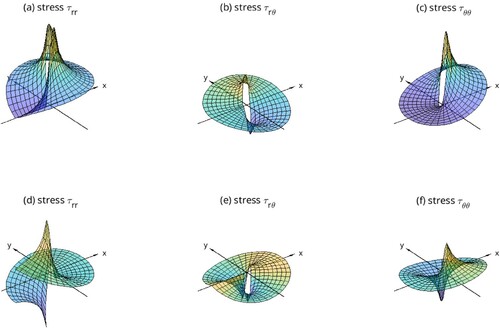
The asymptotic stresses ${\tau }_{rr},{\tau }_{r\theta },{\tau }_{\theta \theta }$ corresponding to the dominate singular term in (87(87) $\begin{array}{rl}\mathbf{u}(r,\theta )-\mathbf{u}(\mathbf{0})& =r^{1/2}[U_3^0\left(\begin{array}{c}3\cos {\displaystyle \frac{3\theta }{2}}+\cos {\displaystyle \frac{\theta }{2}}\\ -3\sin {\displaystyle \frac{3\theta }{2}}-3\sin {\displaystyle \frac{\theta }{2}}\end{array}\right)\\ & +U_4^0\left(\begin{array}{c}-\sin {\displaystyle \frac{3\theta }{2}}-\sin {\displaystyle \frac{\theta }{2}}\\ -\cos {\displaystyle \frac{3\theta }{2}}-3\cos {\displaystyle \frac{\theta }{2}}\end{array}\right)]+\text{O}(r^{3/2}),\end{array}$(87) ) are depicted around the crack tip in Figure 2 for $U_4^0=0$ in plots (a)–(c), and for $U_3^0=0$ in plots (d)–(f).

Figure 2. Singular stresses ${\tau }_{rr},{\tau }_{r\theta },{\tau }_{\theta \theta }$ in the Dirichlet crack problem for Stokes equations in plots (a)–(c) as the stress intensity factors $U_3^0=1,U_4^0=0$, and in plots (d)–(f) as $U_3^0=0,U_4^0=1$.

4.2. Crack under mixed Dirichlet–Neumann impermeability condition

Because in the polar coordinates the normal displacement at the crack is $\mathbf{u}\cdot \mathbf{n}=-u_{\theta }$, and the tangential stress is $\mathit{\tau }-(\mathit{\tau }\cdot \mathbf{n})\mathbf{n}={\tau }_{r\theta }$, the mixed Dirichlet–Neumann boundary conditions in (6(6) $\begin{array}{r}[[\mathbf{u}\cdot \mathbf{n}]]=\{\{\mathbf{u}\cdot \mathbf{n}\}\}=0,[[\mathit{\tau }-(\mathit{\tau }\cdot \mathbf{n})\mathbf{n}]]=\{\{\mathit{\tau }-(\mathit{\tau }\cdot \mathbf{n})\mathbf{n}\}\}=\mathbf{0},\end{array}$(6) ) imply the following pairs of equations $[[{\mathrm{\Psi }}_{\theta }^0]]=[[S_{r\theta }^0]]=0$ and $\{\{{\mathrm{\Psi }}_{\theta }^0\}\}=\{\{S_{r\theta }^0\}\}=0$. According to their representation in (71(71) $\begin{array}{rl}[[{\mathrm{\Psi }}_{\theta }^0]]& =2(U_1^0+\frac{\gamma +1}{\gamma -1}{U}_3^0)\sin \gamma \pi ,\{\{{\mathrm{\Psi }}_{\theta }^0\}\}=-(U_2^0+\frac{\gamma +1}{\gamma -1}{U}_4^0)\cos \gamma \pi ,\end{array}$(71) ) and (72(72) $\begin{array}{rl}[[S_{r\theta }^0]]& =4\mu \gamma (U_1^0+U_3^0)\sin \gamma \pi ,\{\{S_{r\theta }^0\}\}=-2\mu \gamma (U_2^0+U_4^0)\cos \gamma \pi ,\end{array}$(72) ), we get two matrix equations: (88) $\begin{array}{rl}& \left(\begin{array}{cc}2\sin \gamma \pi & 2{\displaystyle \frac{\gamma +1}{\gamma -1}}\sin \gamma \pi \\ 4\mu \gamma \sin \gamma \pi & 4\mu \gamma \sin \gamma \pi \end{array}\right)\left(\begin{array}{c}{U}_1^0\\ U_3^0\end{array}\right)=\left(\begin{array}{c}0\\ 0\end{array}\right),\\ & \left(\begin{array}{cc}-\cos \gamma \pi & -{\displaystyle \frac{\gamma +1}{\gamma -1}}\cos \gamma \pi \\ -2\mu \gamma \cos \gamma \pi & -2\mu \gamma \cos \gamma \pi \end{array}\right)\left(\begin{array}{c}{U}_2^0\\ U_4^0\end{array}\right)=\left(\begin{array}{c}0\\ 0\end{array}\right),\end{array}$(88) which solvability necessitates again the condition (79(79) $\begin{array}{r}\sin (2\gamma \pi )=0,\end{array}$(79) ), half-integer powers (80(80) $\begin{array}{r}\gamma =\frac{n}{2}\text{for integer }n\in \mathbb{Z}.\end{array}$(80) ), and admissible solutions (89) $\begin{array}{r}\{\begin{array}{ll}\cos \gamma \pi =0:& U_1^0=U_3^0=0,\\ \sin \gamma \pi =0,\gamma \ne 0,1:& U_2^0=U_4^0=0,\\ \gamma =0:& U_2^0-U_4^0=0,\\ \gamma =1:& U_2^0=U_3^0=U_4^0=0.\end{array}\end{array}$(89) Here, if $\gamma =1$, then $U_3^0=U_4^0=0$ holds together with $U_2^0=0$ in (88(88) $\begin{array}{rl}& \left(\begin{array}{cc}2\sin \gamma \pi & 2{\displaystyle \frac{\gamma +1}{\gamma -1}}\sin \gamma \pi \\ 4\mu \gamma \sin \gamma \pi & 4\mu \gamma \sin \gamma \pi \end{array}\right)\left(\begin{array}{c}{U}_1^0\\ U_3^0\end{array}\right)=\left(\begin{array}{c}0\\ 0\end{array}\right),\\ & \left(\begin{array}{cc}-\cos \gamma \pi & -{\displaystyle \frac{\gamma +1}{\gamma -1}}\cos \gamma \pi \\ -2\mu \gamma \cos \gamma \pi & -2\mu \gamma \cos \gamma \pi \end{array}\right)\left(\begin{array}{c}{U}_2^0\\ U_4^0\end{array}\right)=\left(\begin{array}{c}0\\ 0\end{array}\right),\end{array}$(88) ).

As m = 1, equations $[[{\mathrm{\Psi }}_{\theta }^1]]=[[S_{r\theta }^1]]=0$ and $\{\{{\mathrm{\Psi }}_{\theta }^1\}\}=\{\{S_{r\theta }^1\}\}=0$ according to (75(75) $\begin{array}{rl}[[{\mathrm{\Psi }}_{\theta }^1]]& =2[U_1^1+\frac{\gamma +1}{\gamma -1}{U}_3^1-\frac{2}{(\gamma -1{)}^2}{U}_3^0]\sin \gamma \pi +2\pi (U_1^0+\frac{\gamma +1}{\gamma -1}{U}_3^0)\cos \gamma \pi ,\\ \{\{{\mathrm{\Psi }}_{\theta }^1\}\}& =-[U_2^1+\frac{\gamma +1}{\gamma -1}{U}_4^1-\frac{2}{(\gamma -1{)}^2}{U}_4^0]\cos \gamma \pi +\pi (U_2^0+\frac{\gamma +1}{\gamma -1}{U}_4^0)\sin \gamma \pi ,\end{array}$(75) ) and (76(76) $\begin{array}{rl}[[S_{r\theta }^1]]& =4\mu (\gamma (U_1^1+U_3^1)+U_1^0+U_3^0)\sin \gamma \pi +4\mu \gamma \pi (U_1^0+U_3^0)\cos \gamma \pi ,\\ \{\{S_{r\theta }^1\}\}& =-2\mu (\gamma (U_2^1+U_4^1)+U_2^0+U_4^0)\cos \gamma \pi +2\mu \gamma \pi (U_2^0+U_4^0)\sin \gamma \pi ,\end{array}$(76) ) read (90) $\begin{array}{rl}& \left(\begin{array}{cc}2\sin \gamma \pi & 2{\displaystyle \frac{\gamma +1}{\gamma -1}}\sin \gamma \pi \\ 4\mu \gamma \sin \gamma \pi & 4\mu \gamma \sin \gamma \pi \end{array}\right)\left(\begin{array}{c}{U}_1^1\\ U_3^1\end{array}\right)\\ & =\left(\begin{array}{c}-2\pi (U_1^0+{\displaystyle \frac{\gamma +1}{\gamma -1}}{U}_3^0)\cos \gamma \pi +{\displaystyle \frac{4}{(\gamma -1{)}^2}}{U}_3^0\sin \gamma \pi \\ -4\mu (U_1^0+U_3^0)\sin \gamma \pi -4\mu \gamma \pi (U_1^0+U_3^0)\cos \gamma \pi \end{array}\right),\\ & \left(\begin{array}{cc}-\cos \gamma \pi & -{\displaystyle \frac{\gamma +1}{\gamma -1}}\cos \gamma \pi \\ -2\mu \gamma \cos \gamma \pi & -2\mu \gamma \cos \gamma \pi \end{array}\right)\left(\begin{array}{c}{U}_2^1\\ U_4^1\end{array}\right)\\ & =\left(\begin{array}{c}-\pi (U_2^0+{\displaystyle \frac{\gamma +1}{\gamma -1}}{U}_4^0)\sin \gamma \pi -{\displaystyle \frac{4}{(\gamma -1{)}^2}}{U}_4^0\cos \gamma \pi \\ 2\mu (U_2^0+U_4^0)\cos \gamma \pi -2\mu \gamma \pi (U_2^0+U_4^0)\sin \gamma \pi \end{array}\right),\end{array}$(90) and they are solvable when (91) $\begin{array}{r}\{\begin{array}{ll}\cos \gamma \pi =0:& U_2^0=U_4^0=0,\\ \sin \gamma \pi =0,\gamma \ne 0,1:& U_1^0=U_3^0=0,\\ \gamma =0:& U_1^0-U_3^0=0,U_2^0+U_4^0=0,\\ \gamma =1:& U_1^0=U_3^0=U_4^0=0.\end{array}\end{array}$(91) From (90(90) $\begin{array}{rl}& \left(\begin{array}{cc}2\sin \gamma \pi & 2{\displaystyle \frac{\gamma +1}{\gamma -1}}\sin \gamma \pi \\ 4\mu \gamma \sin \gamma \pi & 4\mu \gamma \sin \gamma \pi \end{array}\right)\left(\begin{array}{c}{U}_1^1\\ U_3^1\end{array}\right)\\ & =\left(\begin{array}{c}-2\pi (U_1^0+{\displaystyle \frac{\gamma +1}{\gamma -1}}{U}_3^0)\cos \gamma \pi +{\displaystyle \frac{4}{(\gamma -1{)}^2}}{U}_3^0\sin \gamma \pi \\ -4\mu (U_1^0+U_3^0)\sin \gamma \pi -4\mu \gamma \pi (U_1^0+U_3^0)\cos \gamma \pi \end{array}\right),\\ & \left(\begin{array}{cc}-\cos \gamma \pi & -{\displaystyle \frac{\gamma +1}{\gamma -1}}\cos \gamma \pi \\ -2\mu \gamma \cos \gamma \pi & -2\mu \gamma \cos \gamma \pi \end{array}\right)\left(\begin{array}{c}{U}_2^1\\ U_4^1\end{array}\right)\\ & =\left(\begin{array}{c}-\pi (U_2^0+{\displaystyle \frac{\gamma +1}{\gamma -1}}{U}_4^0)\sin \gamma \pi -{\displaystyle \frac{4}{(\gamma -1{)}^2}}{U}_4^0\cos \gamma \pi \\ 2\mu (U_2^0+U_4^0)\cos \gamma \pi -2\mu \gamma \pi (U_2^0+U_4^0)\sin \gamma \pi \end{array}\right),\end{array}$(90) ) and (91(91) $\begin{array}{r}\{\begin{array}{ll}\cos \gamma \pi =0:& U_2^0=U_4^0=0,\\ \sin \gamma \pi =0,\gamma \ne 0,1:& U_1^0=U_3^0=0,\\ \gamma =0:& U_1^0-U_3^0=0,U_2^0+U_4^0=0,\\ \gamma =1:& U_1^0=U_3^0=U_4^0=0.\end{array}\end{array}$(91) ) we infer that no logarithms occur except for $\gamma =0$.

Theorem 4.2

(Power series for the impermeability crack problem). The Stokes equation (18(18) $\begin{array}{r}{\tau }_{rr,r}+\frac{1}{r}{\tau }_{rr}+\frac{1}{r}{\tau }_{r\theta ,\theta }-\frac{1}{r}{\tau }_{\theta \theta }=0,{\tau }_{r\theta ,r}+\frac{2}{r}{\tau }_{r\theta }+\frac{1}{r}{\tau }_{\theta \theta ,\theta }=0,{\epsilon }_{rr}(\mathbf{u})+{\epsilon }_{\theta \theta }(\mathbf{u})=0.\end{array}$(18) ) with the crack under mixed Dirichlet–Neumann impermeability conditions (6(6) $\begin{array}{r}[[\mathbf{u}\cdot \mathbf{n}]]=\{\{\mathbf{u}\cdot \mathbf{n}\}\}=0,[[\mathit{\tau }-(\mathit{\tau }\cdot \mathbf{n})\mathbf{n}]]=\{\{\mathit{\tau }-(\mathit{\tau }\cdot \mathbf{n})\mathbf{n}\}\}=\mathbf{0},\end{array}$(6) ) have the power series solution: (92) $\begin{array}{r}\mathbf{u}(r,\theta )-{\mathbf{u}}^0(r,\theta )=\sum _{n\in \mathbb{Z}\setminus \{0\}}{r}^{n/2}{\mathbf{\Psi }}^0(\frac{n}{2},\theta ),p(r,\theta )=\sum _{n\in \mathbb{Z}\setminus \{0\}}{r}^{n/2-1}{\mathrm{\Phi }}^0(\frac{n}{2},\theta ),\end{array}$(92) since ${\mathrm{\Phi }}^0(0,\theta )\equiv 0$, and ${\mathbf{u}}^0(r,\theta )$ is determined according to (56(56) $\begin{array}{rl}\mathbf{u}(r,\theta )& =\sum _{\gamma \in \mathbb{R}}{\mathbf{u}}^{\gamma },{\mathbf{u}}^{\gamma }(r,\theta )=r^{\gamma }\sum _{m=0}^{M(\gamma )}\frac{(\ln r{)}^{M(\gamma )-m}}{(M(\gamma )-m)!}{\mathbf{\Psi }}^m(\gamma ,\theta ),\\ p(r,\theta )& =\sum _{\gamma \in \mathbb{R}\setminus \{0\}}{p}^{\gamma },p^{\gamma }(r,\theta )=r^{\gamma -1}\sum _{m=0}^{M(\gamma )}\frac{(\ln r{)}^{M(\gamma )-m}}{(M(\gamma )-m)!}{\mathrm{\Phi }}^m(\gamma ,\theta ),\end{array}$(56) ) and (57(57) $\begin{array}{rl}{\mathbf{\Psi }}^0& =\sum _{l=1}^4{U}_l^0{\mathit{\psi }}_l(\gamma ,\theta ),{\mathbf{\Psi }}^m=\sum _{l=1}^4{U}_l^m{\mathit{\psi }}_l(\gamma ,\theta )-\sum _{i=1}^m\frac{(-1{)}^i}{i!}\frac{{\mathrm{\partial }}^i{\mathbf{\Psi }}^{m-i}}{\mathrm{\partial }{\gamma }^i},\end{array}$(57) ) at $\gamma =n/2=0$. For $n\ne 0$, the functions ${\mathbf{\Psi }}^0$ and ${\mathrm{\Phi }}^0$ are given in (85(85) $\begin{array}{r}{\mathbf{\Psi }}^0(\frac{n}{2},\theta )=\sum _{l=1}^4{U}_l^0{\mathit{\psi }}_l(\frac{n}{2},\theta ),{\mathrm{\Phi }}^0(\frac{n}{2},\theta )=\sum _{l=3}^4{P}_l^0{\varphi }_l(\frac{n}{2},\theta ),\end{array}$(85) ) involving the six coefficients $U_1^0,\dots ,U_4^0,P_3^0,P_4^0\in \mathbb{R}$ as follows: (93) $\begin{array}{r}\{\begin{array}{ll}n=2k-1:& U_1^0=U_3^0=0,\\ n=2k,k\ne 0,1:& U_2^0=U_4^0=0,\\ n=2:& U_2^0=U_3^0=U_4^0=0,\end{array}4\mu n{U}_l^0=(n-2)P_l^0\text{for }l=3,4.\end{array}$(93) For the variational solution n>0, the crack singularity has the explicit form as n = k = 1 in (93(93) $\begin{array}{r}\{\begin{array}{ll}n=2k-1:& U_1^0=U_3^0=0,\\ n=2k,k\ne 0,1:& U_2^0=U_4^0=0,\\ n=2:& U_2^0=U_3^0=U_4^0=0,\end{array}4\mu n{U}_l^0=(n-2)P_l^0\text{for }l=3,4.\end{array}$(93) ): (94) $\begin{array}{r}\mathbf{u}(r,\theta )-\mathbf{u}(\mathbf{0})=r^{1/2}[U_2^0\left(\begin{array}{c}\sin {\displaystyle \frac{3\theta }{2}}\\ \cos {\displaystyle \frac{3\theta }{2}}\end{array}\right)+U_4^0\left(\begin{array}{c}-\sin {\displaystyle \frac{\theta }{2}}\\ -3\cos {\displaystyle \frac{\theta }{2}}\end{array}\right)]+\text{O}(r),\end{array}$(94) the pressure and stresses $\begin{array}{rl}p& =4\mu r^{-1/2}{U}_4^0\sin \frac{\theta }{2}+\text{O}(1),{\tau }_{rr}=\mu r^{-1/2}(U_2^0\sin \frac{3\theta }{2}-5U_4^0\sin \frac{\theta }{2})+\text{O}(1),\\ {\tau }_{r\theta }& =\mu r^{-1/2}(U_2^0\cos \frac{3\theta }{2}+U_4^0\cos \frac{\theta }{2})+\text{O}(1),\\ {\tau }_{\theta \theta }& =\mu r^{-1/2}(-U_2^0\sin \frac{3\theta }{2}-3U_4^0\sin \frac{\theta }{2})+\text{O}(1),\end{array}$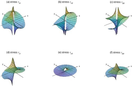which are depicted in Figure 3 for $U_4^0=0$ in plots (a)–(c), and for $U_2^0=0$ in plots (d)–(f).

Figure 3. Singular stresses ${\tau }_{rr},{\tau }_{r\theta },{\tau }_{\theta \theta }$ in the Dirichlet–Neumann crack problem for Stokes equations in plots (a)–(c) as the stress intensity factors $U_2^0=1,U_4^0=0$, and in plots (d)–(f) as $U_2^0=0,U_4^0=1$.

4.3. Stress-free crack under Neumann conditions

The four equations constituting homogeneous Neumann boundary conditions (7(7) $\begin{array}{r}[[\mathit{\tau }]]=\{\{\mathit{\tau }\}\}=\mathbf{0},\end{array}$(7) ) are decoupled into two pairs, using expressions (72(72) $\begin{array}{rl}[[S_{r\theta }^0]]& =4\mu \gamma (U_1^0+U_3^0)\sin \gamma \pi ,\{\{S_{r\theta }^0\}\}=-2\mu \gamma (U_2^0+U_4^0)\cos \gamma \pi ,\end{array}$(72) ) and (73(73) $\begin{array}{rl}[[S_{\theta \theta }^0]]& =4\mu \gamma (U_2^0+\frac{\gamma +1}{\gamma -1}{U}_4^0)\sin \gamma \pi ,\{\{S_{\theta \theta }^0\}\}=2\mu \gamma (U_1^0+\frac{\gamma +1}{\gamma -1}{U}_3^0)\cos \gamma \pi ,\end{array}$(73) ) as m = 0 for $[[S_{r\theta }^0]]=\{\{S_{\theta \theta }^0\}\}=0$ and $\{\{S_{r\theta }^0\}\}=[[S_{\theta \theta }^0]]=0$: (95) $\begin{array}{rl}& \left(\begin{array}{cc}4\mu \gamma \sin \gamma \pi & 4\mu \gamma \sin \gamma \pi \\ 2\mu \gamma \cos \gamma \pi & 2\mu \gamma {\displaystyle \frac{\gamma +1}{\gamma -1}}\cos \gamma \pi \end{array}\right)\left(\begin{array}{c}{U}_1^0\\ U_3^0\end{array}\right)=\left(\begin{array}{c}0\\ 0\end{array}\right),\\ & \left(\begin{array}{cc}-2\mu \gamma \cos \gamma \pi & -2\mu \gamma \cos \gamma \pi \\ 4\mu \gamma \sin \gamma \pi & 4\mu \gamma {\displaystyle \frac{\gamma +1}{\gamma -1}}\sin \gamma \pi \end{array}\right)\left(\begin{array}{c}{U}_2^0\\ U_4^0\end{array}\right)=\left(\begin{array}{c}0\\ 0\end{array}\right).\end{array}$(95) Zero matrix determinant in (95(95) $\begin{array}{rl}& \left(\begin{array}{cc}4\mu \gamma \sin \gamma \pi & 4\mu \gamma \sin \gamma \pi \\ 2\mu \gamma \cos \gamma \pi & 2\mu \gamma {\displaystyle \frac{\gamma +1}{\gamma -1}}\cos \gamma \pi \end{array}\right)\left(\begin{array}{c}{U}_1^0\\ U_3^0\end{array}\right)=\left(\begin{array}{c}0\\ 0\end{array}\right),\\ & \left(\begin{array}{cc}-2\mu \gamma \cos \gamma \pi & -2\mu \gamma \cos \gamma \pi \\ 4\mu \gamma \sin \gamma \pi & 4\mu \gamma {\displaystyle \frac{\gamma +1}{\gamma -1}}\sin \gamma \pi \end{array}\right)\left(\begin{array}{c}{U}_2^0\\ U_4^0\end{array}\right)=\left(\begin{array}{c}0\\ 0\end{array}\right).\end{array}$(95) ) leads to γ in (79(79) $\begin{array}{r}\sin (2\gamma \pi )=0,\end{array}$(79) ) and (80(80) $\begin{array}{r}\gamma =\frac{n}{2}\text{for integer }n\in \mathbb{Z}.\end{array}$(80) ), such that admissible coefficients are (96) $\begin{array}{r}\{\begin{array}{ll}\cos \gamma \pi =0:& U_1^0+U_3^0=0,U_2^0+{\displaystyle \frac{\gamma +1}{\gamma -1}}{U}_4^0=0,\\ \sin \gamma \pi =0,\gamma \ne 0,1:& U_1^0+{\displaystyle \frac{\gamma +1}{\gamma -1}}{U}_3^0=0,U_2^0+U_4^0=0,\\ \gamma =0:& \text{arbitrary }{U}_1^0,U_2^0,U_3^0,U_4^0,\\ \gamma =1:& U_1^0=U_2^0=U_3^0=U_4^0=0,\end{array}\end{array}$(96) where $U_3^0=U_4^0=0$ as $\gamma =1$ was used from Theorem 3.1.

For m = 1, equations $[[S_{r\theta }^1]]=\{\{S_{\theta \theta }^1\}\}=0$ and $\{\{S_{r\theta }^1\}\}=[[S_{\theta \theta }^1]]=0$ in (76(76) $\begin{array}{rl}[[S_{r\theta }^1]]& =4\mu (\gamma (U_1^1+U_3^1)+U_1^0+U_3^0)\sin \gamma \pi +4\mu \gamma \pi (U_1^0+U_3^0)\cos \gamma \pi ,\\ \{\{S_{r\theta }^1\}\}& =-2\mu (\gamma (U_2^1+U_4^1)+U_2^0+U_4^0)\cos \gamma \pi +2\mu \gamma \pi (U_2^0+U_4^0)\sin \gamma \pi ,\end{array}$(76) ) and (77(77) $\begin{array}{rl}[[S_{\theta \theta }^1]]& =4\mu [\gamma (U_2^1+\frac{\gamma +1}{\gamma -1}{U}_4^1)+U_2^0+U_4^0]\sin \gamma \pi \\ & +4\mu \gamma \pi (U_2^0+\frac{\gamma +1}{\gamma -1}{U}_4^0)\cos \gamma \pi ,\\ \{\{S_{\theta \theta }^1\}\}& =2\mu [\gamma (U_1^1+\frac{\gamma +1}{\gamma -1}{U}_3^1)+U_1^0+U_3^0]\cos \gamma \pi \\ & -2\mu \gamma \pi (U_1^0+\frac{\gamma +1}{\gamma -1}{U}_3^0)\sin \gamma \pi .\end{array}$(77) ) read: (97) $\begin{array}{rl}& \left(\begin{array}{cc}4\mu \gamma \sin \gamma \pi & 4\mu \gamma \sin \gamma \pi \\ 2\mu \gamma \cos \gamma \pi & 2\mu \gamma {\displaystyle \frac{\gamma +1}{\gamma -1}}\cos \gamma \pi \end{array}\right)\left(\begin{array}{c}{U}_1^1\\ U_3^1\end{array}\right)\\ & =\left(\begin{array}{c}-4\mu (U_1^0+U_3^0)\sin \gamma \pi -4\mu \gamma \pi (U_1^0+U_3^0)\cos \gamma \pi \\ -2\mu (U_1^0+U_3^0)\cos \gamma \pi +2\mu \gamma \pi (U_1^0+{\displaystyle \frac{\gamma +1}{\gamma -1}}{U}_3^0)\sin \gamma \pi \end{array}\right),\\ & \left(\begin{array}{cc}-2\mu \gamma \cos \gamma \pi & -2\mu \gamma \cos \gamma \pi \\ 4\mu \gamma \sin \gamma \pi & 4\mu \gamma {\displaystyle \frac{\gamma +1}{\gamma -1}}\sin \gamma \pi \end{array}\right)\left(\begin{array}{c}{U}_2^1\\ U_4^1\end{array}\right)\\ & =\left(\begin{array}{c}2\mu (U_2^0+U_4^0)\cos \gamma \pi -2\mu \gamma \pi (U_2^0+U_4^0)\sin \gamma \pi \\ -4\mu (U_2^0+U_4^0)\sin \gamma \pi -4\mu \gamma \pi (U_2^0+{\displaystyle \frac{\gamma +1}{\gamma -1}}{U}_4^0)\cos \gamma \pi \end{array}\right).\end{array}$(97) The inhomogeneous system (97(97) $\begin{array}{rl}& \left(\begin{array}{cc}4\mu \gamma \sin \gamma \pi & 4\mu \gamma \sin \gamma \pi \\ 2\mu \gamma \cos \gamma \pi & 2\mu \gamma {\displaystyle \frac{\gamma +1}{\gamma -1}}\cos \gamma \pi \end{array}\right)\left(\begin{array}{c}{U}_1^1\\ U_3^1\end{array}\right)\\ & =\left(\begin{array}{c}-4\mu (U_1^0+U_3^0)\sin \gamma \pi -4\mu \gamma \pi (U_1^0+U_3^0)\cos \gamma \pi \\ -2\mu (U_1^0+U_3^0)\cos \gamma \pi +2\mu \gamma \pi (U_1^0+{\displaystyle \frac{\gamma +1}{\gamma -1}}{U}_3^0)\sin \gamma \pi \end{array}\right),\\ & \left(\begin{array}{cc}-2\mu \gamma \cos \gamma \pi & -2\mu \gamma \cos \gamma \pi \\ 4\mu \gamma \sin \gamma \pi & 4\mu \gamma {\displaystyle \frac{\gamma +1}{\gamma -1}}\sin \gamma \pi \end{array}\right)\left(\begin{array}{c}{U}_2^1\\ U_4^1\end{array}\right)\\ & =\left(\begin{array}{c}2\mu (U_2^0+U_4^0)\cos \gamma \pi -2\mu \gamma \pi (U_2^0+U_4^0)\sin \gamma \pi \\ -4\mu (U_2^0+U_4^0)\sin \gamma \pi -4\mu \gamma \pi (U_2^0+{\displaystyle \frac{\gamma +1}{\gamma -1}}{U}_4^0)\cos \gamma \pi \end{array}\right).\end{array}$(97) ) is solvable when (98) $\begin{array}{r}\{\begin{array}{ll}\cos \gamma \pi =0:& U_1^0+{\displaystyle \frac{\gamma +1}{\gamma -1}}{U}_3^0=0,U_2^0+U_4^0=0,\\ \sin \gamma \pi =0,\gamma \ne 0,1:& U_1^0+U_3^0=0,U_2^0+{\displaystyle \frac{\gamma +1}{\gamma -1}}{U}_4^0=0,\\ \gamma =0:& U_1^0+U_3^0=0,U_2^0+U_4^0=0.\end{array}\end{array}$(98) Together with (96(96) $\begin{array}{r}\{\begin{array}{ll}\cos \gamma \pi =0:& U_1^0+U_3^0=0,U_2^0+{\displaystyle \frac{\gamma +1}{\gamma -1}}{U}_4^0=0,\\ \sin \gamma \pi =0,\gamma \ne 0,1:& U_1^0+{\displaystyle \frac{\gamma +1}{\gamma -1}}{U}_3^0=0,U_2^0+U_4^0=0,\\ \gamma =0:& \text{arbitrary }{U}_1^0,U_2^0,U_3^0,U_4^0,\\ \gamma =1:& U_1^0=U_2^0=U_3^0=U_4^0=0,\end{array}\end{array}$(96) ), conditions (98(98) $\begin{array}{r}\{\begin{array}{ll}\cos \gamma \pi =0:& U_1^0+{\displaystyle \frac{\gamma +1}{\gamma -1}}{U}_3^0=0,U_2^0+U_4^0=0,\\ \sin \gamma \pi =0,\gamma \ne 0,1:& U_1^0+U_3^0=0,U_2^0+{\displaystyle \frac{\gamma +1}{\gamma -1}}{U}_4^0=0,\\ \gamma =0:& U_1^0+U_3^0=0,U_2^0+U_4^0=0.\end{array}\end{array}$(98) ) imply $U_1^0=U_2^0=U_3^0=U_4^0=0$ for $\gamma \ne 0$ and the next theorem.

Theorem 4.3

(Power series for the Neumann crack problem). The Stokes equation (18(18) $\begin{array}{r}{\tau }_{rr,r}+\frac{1}{r}{\tau }_{rr}+\frac{1}{r}{\tau }_{r\theta ,\theta }-\frac{1}{r}{\tau }_{\theta \theta }=0,{\tau }_{r\theta ,r}+\frac{2}{r}{\tau }_{r\theta }+\frac{1}{r}{\tau }_{\theta \theta ,\theta }=0,{\epsilon }_{rr}(\mathbf{u})+{\epsilon }_{\theta \theta }(\mathbf{u})=0.\end{array}$(18) ) under the stress-free crack conditions (7(7) $\begin{array}{r}[[\mathit{\tau }]]=\{\{\mathit{\tau }\}\}=\mathbf{0},\end{array}$(7) ) have the power series solution: (99) $\begin{array}{r}\mathbf{u}(r,\theta )-{\mathbf{u}}^0(r,\theta )=\sum _{n\in \mathbb{Z}\setminus \{0,2\}}{r}^{n/2}{\mathbf{\Psi }}^0(\frac{n}{2},\theta ),p(r,\theta )=\sum _{n\in \mathbb{Z}\setminus \{0\}}{r}^{n/2-1}{\mathrm{\Phi }}^0(\frac{n}{2},\theta ),\end{array}$(99) where ${\mathbf{u}}^0(r,\theta )$ is determined according to (56(56) $\begin{array}{rl}\mathbf{u}(r,\theta )& =\sum _{\gamma \in \mathbb{R}}{\mathbf{u}}^{\gamma },{\mathbf{u}}^{\gamma }(r,\theta )=r^{\gamma }\sum _{m=0}^{M(\gamma )}\frac{(\ln r{)}^{M(\gamma )-m}}{(M(\gamma )-m)!}{\mathbf{\Psi }}^m(\gamma ,\theta ),\\ p(r,\theta )& =\sum _{\gamma \in \mathbb{R}\setminus \{0\}}{p}^{\gamma },p^{\gamma }(r,\theta )=r^{\gamma -1}\sum _{m=0}^{M(\gamma )}\frac{(\ln r{)}^{M(\gamma )-m}}{(M(\gamma )-m)!}{\mathrm{\Phi }}^m(\gamma ,\theta ),\end{array}$(56) ) and (57(57) $\begin{array}{rl}{\mathbf{\Psi }}^0& =\sum _{l=1}^4{U}_l^0{\mathit{\psi }}_l(\gamma ,\theta ),{\mathbf{\Psi }}^m=\sum _{l=1}^4{U}_l^m{\mathit{\psi }}_l(\gamma ,\theta )-\sum _{i=1}^m\frac{(-1{)}^i}{i!}\frac{{\mathrm{\partial }}^i{\mathbf{\Psi }}^{m-i}}{\mathrm{\partial }{\gamma }^i},\end{array}$(57) ). The angular functions for $n\ne 0$ are defined in (85(85) $\begin{array}{r}{\mathbf{\Psi }}^0(\frac{n}{2},\theta )=\sum _{l=1}^4{U}_l^0{\mathit{\psi }}_l(\frac{n}{2},\theta ),{\mathrm{\Phi }}^0(\frac{n}{2},\theta )=\sum _{l=3}^4{P}_l^0{\varphi }_l(\frac{n}{2},\theta ),\end{array}$(85) ) and (60(60) $\begin{array}{r}{\mathit{\psi }}_1=\left(\begin{array}{c}{\varphi }_1\\ -{\varphi }_2\end{array}\right),{\mathit{\psi }}_2=\left(\begin{array}{c}{\varphi }_2\\ {\varphi }_1\end{array}\right),{\mathit{\psi }}_3=\left(\begin{array}{c}{\varphi }_3\\ -{\displaystyle \frac{\gamma +1}{\gamma -1}}{\varphi }_4\end{array}\right),{\mathit{\psi }}_4=\left(\begin{array}{c}{\varphi }_4\\ {\displaystyle \frac{\gamma +1}{\gamma -1}}{\varphi }_3\end{array}\right).\end{array}$(60) ) as $\gamma =n/2$, with the coefficients determined according to formula (96(96) $\begin{array}{r}\{\begin{array}{ll}\cos \gamma \pi =0:& U_1^0+U_3^0=0,U_2^0+{\displaystyle \frac{\gamma +1}{\gamma -1}}{U}_4^0=0,\\ \sin \gamma \pi =0,\gamma \ne 0,1:& U_1^0+{\displaystyle \frac{\gamma +1}{\gamma -1}}{U}_3^0=0,U_2^0+U_4^0=0,\\ \gamma =0:& \text{arbitrary }{U}_1^0,U_2^0,U_3^0,U_4^0,\\ \gamma =1:& U_1^0=U_2^0=U_3^0=U_4^0=0,\end{array}\end{array}$(96) ) for $k\in \mathbb{Z}$: (100) $\begin{array}{r}\{\begin{array}{ll}n=2k-1:& U_1^0+U_3^0=0,\\ & U_2^0+{\displaystyle \frac{2k+1}{2k-3}}{U}_4^0=0,\\ n=2k,k\ne 0,2:& U_1^0+{\displaystyle \frac{k+1}{k-1}}{U}_3^0=0,\\ & U_2^0+U_4^0=0,\end{array}4\mu n{U}_l^0=(n-2)P_l^0\text{for }l=3,4.\end{array}$(100) For the variational solution as n>0, the crack-tip singularity as $r\to 0$ is expressed explicitly: (101) $\begin{array}{r}\mathbf{u}(r,\theta )-\mathbf{u}(\mathbf{0})=r^{1/2}\left[U_3^0\left(\begin{array}{c}-\cos {\displaystyle \frac{3\theta }{2}}+\cos {\displaystyle \frac{\theta }{2}}\\ \sin {\displaystyle \frac{3\theta }{2}}-3\sin {\displaystyle \frac{\theta }{2}}\end{array}\right)+U_4^0\left(\begin{array}{c}3\sin {\displaystyle \frac{3\theta }{2}}-\sin {\displaystyle \frac{\theta }{2}}\\ 3\cos {\displaystyle \frac{3\theta }{2}}-3\cos {\displaystyle \frac{\theta }{2}}\end{array}\right)\right]+\text{O}(r^{3/2}),\end{array}$(101) when $U_1^0+U_3^0=0$ and $U_2^0-3U_4^0=0$ are set for n = k = 1 in (100(100) $\begin{array}{r}\{\begin{array}{ll}n=2k-1:& U_1^0+U_3^0=0,\\ & U_2^0+{\displaystyle \frac{2k+1}{2k-3}}{U}_4^0=0,\\ n=2k,k\ne 0,2:& U_1^0+{\displaystyle \frac{k+1}{k-1}}{U}_3^0=0,\\ & U_2^0+U_4^0=0,\end{array}4\mu n{U}_l^0=(n-2)P_l^0\text{for }l=3,4.\end{array}$(100) ), and $\gamma =1/2$ in (60(60) $\begin{array}{r}{\mathit{\psi }}_1=\left(\begin{array}{c}{\varphi }_1\\ -{\varphi }_2\end{array}\right),{\mathit{\psi }}_2=\left(\begin{array}{c}{\varphi }_2\\ {\varphi }_1\end{array}\right),{\mathit{\psi }}_3=\left(\begin{array}{c}{\varphi }_3\\ -{\displaystyle \frac{\gamma +1}{\gamma -1}}{\varphi }_4\end{array}\right),{\mathit{\psi }}_4=\left(\begin{array}{c}{\varphi }_4\\ {\displaystyle \frac{\gamma +1}{\gamma -1}}{\varphi }_3\end{array}\right).\end{array}$(60) ). The pressure $p=4\mu r^{-1/2}(-U_3^0\cos \frac{\theta }{2}+U_4^0\sin \frac{\theta }{2})+\text{O}(1)$ and stresses are $\begin{array}{rl}{\tau }_{rr}& =\mu r^{-1/2}[U_3^0(-\cos \frac{3\theta }{2}+5\cos \frac{\theta }{2})+U_4^0(3\sin \frac{3\theta }{2}-5\sin \frac{\theta }{2})]+\text{O}(1),\\ {\tau }_{r\theta }& =\mu r^{-1/2}[U_3^0(\sin \frac{3\theta }{2}+\sin \frac{\theta }{2})+U_4^0(3\cos \frac{3\theta }{2}-2\cos \frac{\theta }{2})]+\text{O}(r^{1/2}),\\ {\tau }_{\theta \theta }& =\mu r^{-1/2}[U_3^0(\cos \frac{3\theta }{2}+3\cos \frac{\theta }{2})+U_4^0(-3\sin \frac{3\theta }{2}-3\sin \frac{\theta }{2})]+\text{O}(1),\end{array}$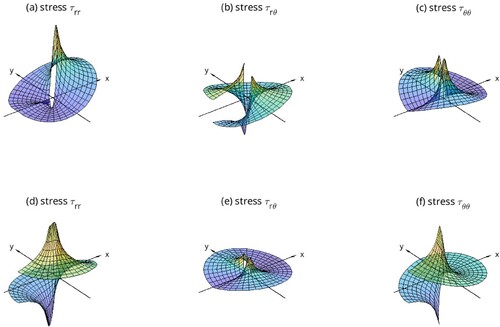as depicted around the crack tip in Figure 4 for $U_4^0=0$ in plots (a)–(c), and for $U_3^0=0$ in plots (d)–(f).

Figure 4. Singular stresses ${\tau }_{rr},{\tau }_{r\theta },{\tau }_{\theta \theta }$ in the Neumann crack problem for Stokes equations in plots (a)–(c) as the stress intensity factors $U_3^0=1,U_4^0=0$, and in plots (d)–(f) as $U_3^0=0,U_4^0=1$.

4.4. Crack under non-penetration conditions

The boundary conditions describing non-penetration between the crack faces (8(8) $\begin{array}{rl}[[\mathit{\tau }-(\mathit{\tau }\cdot \mathbf{n})\mathbf{n}]]& =\{\{\mathit{\tau }-(\mathit{\tau }\cdot \mathbf{n})\mathbf{n}\}\}=\mathbf{0},[[\mathit{\tau }\cdot \mathbf{n}]]=0,[[\mathbf{u}\cdot \mathbf{n}]]\ge 0,\\ \mathit{\tau }\cdot \mathbf{n}& \le 0,[[\mathbf{u}\cdot \mathbf{n}]](\mathit{\tau }\cdot \mathbf{n})=0,\end{array}$(8) ) in the polar coordinates at m = 0 yield as in the Neumann case $\{\{S_{r\theta }^0\}\}=[[S_{\theta \theta }^0]]=0$, hence the second system in (95(95) $\begin{array}{rl}& \left(\begin{array}{cc}4\mu \gamma \sin \gamma \pi & 4\mu \gamma \sin \gamma \pi \\ 2\mu \gamma \cos \gamma \pi & 2\mu \gamma {\displaystyle \frac{\gamma +1}{\gamma -1}}\cos \gamma \pi \end{array}\right)\left(\begin{array}{c}{U}_1^0\\ U_3^0\end{array}\right)=\left(\begin{array}{c}0\\ 0\end{array}\right),\\ & \left(\begin{array}{cc}-2\mu \gamma \cos \gamma \pi & -2\mu \gamma \cos \gamma \pi \\ 4\mu \gamma \sin \gamma \pi & 4\mu \gamma {\displaystyle \frac{\gamma +1}{\gamma -1}}\sin \gamma \pi \end{array}\right)\left(\begin{array}{c}{U}_2^0\\ U_4^0\end{array}\right)=\left(\begin{array}{c}0\\ 0\end{array}\right).\end{array}$(95) ) providing the determinant in (79(79) $\begin{array}{r}\sin (2\gamma \pi )=0,\end{array}$(79) ) and the half-integers powers in (80(80) $\begin{array}{r}\gamma =\frac{n}{2}\text{for integer }n\in \mathbb{Z}.\end{array}$(80) ). The other conditions consisting of $[[S_{r\theta }^0]]=0$ and complementarity relations $\{\{S_{\theta \theta }^0\}\}[[{\mathrm{\Psi }}_{\theta }^0]]=0$, $\{\{S_{\theta \theta }^0\}\}\le 0$, $[[{\mathrm{\Psi }}_{\theta }^0]]\le 0$, using (71(71) $\begin{array}{rl}[[{\mathrm{\Psi }}_{\theta }^0]]& =2(U_1^0+\frac{\gamma +1}{\gamma -1}{U}_3^0)\sin \gamma \pi ,\{\{{\mathrm{\Psi }}_{\theta }^0\}\}=-(U_2^0+\frac{\gamma +1}{\gamma -1}{U}_4^0)\cos \gamma \pi ,\end{array}$(71) )–(73(73) $\begin{array}{rl}[[S_{\theta \theta }^0]]& =4\mu \gamma (U_2^0+\frac{\gamma +1}{\gamma -1}{U}_4^0)\sin \gamma \pi ,\{\{S_{\theta \theta }^0\}\}=2\mu \gamma (U_1^0+\frac{\gamma +1}{\gamma -1}{U}_3^0)\cos \gamma \pi ,\end{array}$(73) ) yield (102) $\begin{array}{rl}& 4\mu \gamma (U_1^0+U_3^0)\sin \gamma \pi =0,2\mu \gamma {(U_1^0+\frac{\gamma +1}{\gamma -1}{U}_3^0)}^2\sin (2\gamma \pi )=0,\\ & 2\mu \gamma (U_1^0+\frac{\gamma +1}{\gamma -1}{U}_3^0)\cos \gamma \pi \le 0,2(U_1^0+\frac{\gamma +1}{\gamma -1}{U}_3^0)\sin \gamma \pi \le 0.\end{array}$(102) The second system in (95(95) $\begin{array}{rl}& \left(\begin{array}{cc}4\mu \gamma \sin \gamma \pi & 4\mu \gamma \sin \gamma \pi \\ 2\mu \gamma \cos \gamma \pi & 2\mu \gamma {\displaystyle \frac{\gamma +1}{\gamma -1}}\cos \gamma \pi \end{array}\right)\left(\begin{array}{c}{U}_1^0\\ U_3^0\end{array}\right)=\left(\begin{array}{c}0\\ 0\end{array}\right),\\ & \left(\begin{array}{cc}-2\mu \gamma \cos \gamma \pi & -2\mu \gamma \cos \gamma \pi \\ 4\mu \gamma \sin \gamma \pi & 4\mu \gamma {\displaystyle \frac{\gamma +1}{\gamma -1}}\sin \gamma \pi \end{array}\right)\left(\begin{array}{c}{U}_2^0\\ U_4^0\end{array}\right)=\left(\begin{array}{c}0\\ 0\end{array}\right).\end{array}$(95) ) for $U_2^0,U_4^0$ and nonlinear relations (102(102) $\begin{array}{rl}& 4\mu \gamma (U_1^0+U_3^0)\sin \gamma \pi =0,2\mu \gamma {(U_1^0+\frac{\gamma +1}{\gamma -1}{U}_3^0)}^2\sin (2\gamma \pi )=0,\\ & 2\mu \gamma (U_1^0+\frac{\gamma +1}{\gamma -1}{U}_3^0)\cos \gamma \pi \le 0,2(U_1^0+\frac{\gamma +1}{\gamma -1}{U}_3^0)\sin \gamma \pi \le 0.\end{array}$(102) ) for $U_1^0,U_3^0$ have admissible solutions (103) $\begin{array}{r}\{\begin{array}{ll}\cos \gamma \pi =0:& U_1^0+U_3^0=0,{\displaystyle \frac{1}{\gamma -1}}{U}_3^0\sin \gamma \pi \le 0,U_2^0+{\displaystyle \frac{\gamma +1}{\gamma -1}}{U}_4^0=0,\\ \sin \gamma \pi =0,\gamma \ne 0,1:& \gamma (U_1^0+{\displaystyle \frac{\gamma +1}{\gamma -1}}{U}_3^0)\cos \gamma \pi \le 0,U_2^0+U_4^0=0,\\ \gamma =0:& \text{arbitrary }{U}_1^0,U_2^0,U_3^0,U_4^0,\\ \gamma =1:& U_1^0\ge 0,U_2^0=U_3^0=U_4^0=0,\end{array}\end{array}$(103) where $U_3^0=U_4^0=0$ at $\gamma =1$ follows $U_1^0\ge 0$ in (102(102) $\begin{array}{rl}& 4\mu \gamma (U_1^0+U_3^0)\sin \gamma \pi =0,2\mu \gamma {(U_1^0+\frac{\gamma +1}{\gamma -1}{U}_3^0)}^2\sin (2\gamma \pi )=0,\\ & 2\mu \gamma (U_1^0+\frac{\gamma +1}{\gamma -1}{U}_3^0)\cos \gamma \pi \le 0,2(U_1^0+\frac{\gamma +1}{\gamma -1}{U}_3^0)\sin \gamma \pi \le 0.\end{array}$(102) ), and $U_2^0=0$ from the second system in (95(95) $\begin{array}{rl}& \left(\begin{array}{cc}4\mu \gamma \sin \gamma \pi & 4\mu \gamma \sin \gamma \pi \\ 2\mu \gamma \cos \gamma \pi & 2\mu \gamma {\displaystyle \frac{\gamma +1}{\gamma -1}}\cos \gamma \pi \end{array}\right)\left(\begin{array}{c}{U}_1^0\\ U_3^0\end{array}\right)=\left(\begin{array}{c}0\\ 0\end{array}\right),\\ & \left(\begin{array}{cc}-2\mu \gamma \cos \gamma \pi & -2\mu \gamma \cos \gamma \pi \\ 4\mu \gamma \sin \gamma \pi & 4\mu \gamma {\displaystyle \frac{\gamma +1}{\gamma -1}}\sin \gamma \pi \end{array}\right)\left(\begin{array}{c}{U}_2^0\\ U_4^0\end{array}\right)=\left(\begin{array}{c}0\\ 0\end{array}\right).\end{array}$(95) ).

At m = 1, linear conditions $\{\{S_{r\theta }^1\}\}=[[S_{\theta \theta }^1]]=0$ imply the second system in (97(97) $\begin{array}{rl}& \left(\begin{array}{cc}4\mu \gamma \sin \gamma \pi & 4\mu \gamma \sin \gamma \pi \\ 2\mu \gamma \cos \gamma \pi & 2\mu \gamma {\displaystyle \frac{\gamma +1}{\gamma -1}}\cos \gamma \pi \end{array}\right)\left(\begin{array}{c}{U}_1^1\\ U_3^1\end{array}\right)\\ & =\left(\begin{array}{c}-4\mu (U_1^0+U_3^0)\sin \gamma \pi -4\mu \gamma \pi (U_1^0+U_3^0)\cos \gamma \pi \\ -2\mu (U_1^0+U_3^0)\cos \gamma \pi +2\mu \gamma \pi (U_1^0+{\displaystyle \frac{\gamma +1}{\gamma -1}}{U}_3^0)\sin \gamma \pi \end{array}\right),\\ & \left(\begin{array}{cc}-2\mu \gamma \cos \gamma \pi & -2\mu \gamma \cos \gamma \pi \\ 4\mu \gamma \sin \gamma \pi & 4\mu \gamma {\displaystyle \frac{\gamma +1}{\gamma -1}}\sin \gamma \pi \end{array}\right)\left(\begin{array}{c}{U}_2^1\\ U_4^1\end{array}\right)\\ & =\left(\begin{array}{c}2\mu (U_2^0+U_4^0)\cos \gamma \pi -2\mu \gamma \pi (U_2^0+U_4^0)\sin \gamma \pi \\ -4\mu (U_2^0+U_4^0)\sin \gamma \pi -4\mu \gamma \pi (U_2^0+{\displaystyle \frac{\gamma +1}{\gamma -1}}{U}_4^0)\cos \gamma \pi \end{array}\right).\end{array}$(97) ). According to (98(98) $\begin{array}{r}\{\begin{array}{ll}\cos \gamma \pi =0:& U_1^0+{\displaystyle \frac{\gamma +1}{\gamma -1}}{U}_3^0=0,U_2^0+U_4^0=0,\\ \sin \gamma \pi =0,\gamma \ne 0,1:& U_1^0+U_3^0=0,U_2^0+{\displaystyle \frac{\gamma +1}{\gamma -1}}{U}_4^0=0,\\ \gamma =0:& U_1^0+U_3^0=0,U_2^0+U_4^0=0.\end{array}\end{array}$(98) ) we find $U_2^0+U_4^0=0$ for $\cos \gamma \pi =0$ or $\gamma =0$, and $U_2^0+\frac{\gamma +1}{\gamma -1}{U}_4^0=0$ for $\sin \gamma \pi =0$ and $\gamma \ne 0,1$. Together with (103(103) $\begin{array}{r}\{\begin{array}{ll}\cos \gamma \pi =0:& U_1^0+U_3^0=0,{\displaystyle \frac{1}{\gamma -1}}{U}_3^0\sin \gamma \pi \le 0,U_2^0+{\displaystyle \frac{\gamma +1}{\gamma -1}}{U}_4^0=0,\\ \sin \gamma \pi =0,\gamma \ne 0,1:& \gamma (U_1^0+{\displaystyle \frac{\gamma +1}{\gamma -1}}{U}_3^0)\cos \gamma \pi \le 0,U_2^0+U_4^0=0,\\ \gamma =0:& \text{arbitrary }{U}_1^0,U_2^0,U_3^0,U_4^0,\\ \gamma =1:& U_1^0\ge 0,U_2^0=U_3^0=U_4^0=0,\end{array}\end{array}$(103) ) this means that logarithms for the eigenvectors ${\varphi }_2$ and ${\varphi }_4$ may appear only if $\gamma =0$.

The nonlinear conditions $[[S_{r\theta }^1]]=0$ and $\{\{S_{\theta \theta }^1\}\}[[{\mathrm{\Psi }}_{\theta }^1]]=0$, $\{\{S_{\theta \theta }^1\}\}\le 0$, $[[{\mathrm{\Psi }}_{\theta }^1]]\le 0$ in (75(75) $\begin{array}{rl}[[{\mathrm{\Psi }}_{\theta }^1]]& =2[U_1^1+\frac{\gamma +1}{\gamma -1}{U}_3^1-\frac{2}{(\gamma -1{)}^2}{U}_3^0]\sin \gamma \pi +2\pi (U_1^0+\frac{\gamma +1}{\gamma -1}{U}_3^0)\cos \gamma \pi ,\\ \{\{{\mathrm{\Psi }}_{\theta }^1\}\}& =-[U_2^1+\frac{\gamma +1}{\gamma -1}{U}_4^1-\frac{2}{(\gamma -1{)}^2}{U}_4^0]\cos \gamma \pi +\pi (U_2^0+\frac{\gamma +1}{\gamma -1}{U}_4^0)\sin \gamma \pi ,\end{array}$(75) ) and (77(77) $\begin{array}{rl}[[S_{\theta \theta }^1]]& =4\mu [\gamma (U_2^1+\frac{\gamma +1}{\gamma -1}{U}_4^1)+U_2^0+U_4^0]\sin \gamma \pi \\ & +4\mu \gamma \pi (U_2^0+\frac{\gamma +1}{\gamma -1}{U}_4^0)\cos \gamma \pi ,\\ \{\{S_{\theta \theta }^1\}\}& =2\mu [\gamma (U_1^1+\frac{\gamma +1}{\gamma -1}{U}_3^1)+U_1^0+U_3^0]\cos \gamma \pi \\ & -2\mu \gamma \pi (U_1^0+\frac{\gamma +1}{\gamma -1}{U}_3^0)\sin \gamma \pi .\end{array}$(77) ), after division by 2 and $2\mu >0$ are (104) $\begin{array}{rl}\gamma (U_1^1+U_3^1)\sin \gamma \pi & =-(U_1^0+U_3^0)(\sin \gamma \pi +\gamma \pi \cos \gamma \pi ),\\ ([\gamma (U_1^1+\frac{\gamma +1}{\gamma -1}{U}_3^1)+U_1^0+U_3^0]\cos \gamma \pi & -\gamma \pi (U_1^0+\frac{\gamma +1}{\gamma -1}{U}_3^0)\sin \gamma \pi )\\ \times ([U_1^1+\frac{\gamma +1}{\gamma -1}{U}_3^1-\frac{2}{(\gamma -1{)}^2}{U}_3^0]\sin \gamma \pi & +\pi (U_1^0+\frac{\gamma +1}{\gamma -1}{U}_3^0)\cos \gamma \pi )=0,\\ \gamma (U_1^1+\frac{\gamma +1}{\gamma -1}{U}_3^1)\cos \gamma \pi & \le -(U_1^0+U_3^0)\cos \gamma \pi \\ & +\gamma \pi (U_1^0+\frac{\gamma +1}{\gamma -1}{U}_3^0)\sin \gamma \pi ,\\ (U_1^1+\frac{\gamma +1}{\gamma -1}{U}_3^1)\sin \gamma \pi & \le \frac{2}{(\gamma -1{)}^2}{U}_3^0\sin \gamma \pi \\ & -\pi (U_1^0+\frac{\gamma +1}{\gamma -1}{U}_3^0)\cos \gamma \pi .\end{array}$(104) If $\cos \gamma \pi =0$ in (104(104) $\begin{array}{rl}\gamma (U_1^1+U_3^1)\sin \gamma \pi & =-(U_1^0+U_3^0)(\sin \gamma \pi +\gamma \pi \cos \gamma \pi ),\\ ([\gamma (U_1^1+\frac{\gamma +1}{\gamma -1}{U}_3^1)+U_1^0+U_3^0]\cos \gamma \pi & -\gamma \pi (U_1^0+\frac{\gamma +1}{\gamma -1}{U}_3^0)\sin \gamma \pi )\\ \times ([U_1^1+\frac{\gamma +1}{\gamma -1}{U}_3^1-\frac{2}{(\gamma -1{)}^2}{U}_3^0]\sin \gamma \pi & +\pi (U_1^0+\frac{\gamma +1}{\gamma -1}{U}_3^0)\cos \gamma \pi )=0,\\ \gamma (U_1^1+\frac{\gamma +1}{\gamma -1}{U}_3^1)\cos \gamma \pi & \le -(U_1^0+U_3^0)\cos \gamma \pi \\ & +\gamma \pi (U_1^0+\frac{\gamma +1}{\gamma -1}{U}_3^0)\sin \gamma \pi ,\\ (U_1^1+\frac{\gamma +1}{\gamma -1}{U}_3^1)\sin \gamma \pi & \le \frac{2}{(\gamma -1{)}^2}{U}_3^0\sin \gamma \pi \\ & -\pi (U_1^0+\frac{\gamma +1}{\gamma -1}{U}_3^0)\cos \gamma \pi .\end{array}$(104) ) for $\gamma =k-1/2$, using $U_1^0+U_3^0=0$ from the first string in (103(103) $\begin{array}{r}\{\begin{array}{ll}\cos \gamma \pi =0:& U_1^0+U_3^0=0,{\displaystyle \frac{1}{\gamma -1}}{U}_3^0\sin \gamma \pi \le 0,U_2^0+{\displaystyle \frac{\gamma +1}{\gamma -1}}{U}_4^0=0,\\ \sin \gamma \pi =0,\gamma \ne 0,1:& \gamma (U_1^0+{\displaystyle \frac{\gamma +1}{\gamma -1}}{U}_3^0)\cos \gamma \pi \le 0,U_2^0+U_4^0=0,\\ \gamma =0:& \text{arbitrary }{U}_1^0,U_2^0,U_3^0,U_4^0,\\ \gamma =1:& U_1^0\ge 0,U_2^0=U_3^0=U_4^0=0,\end{array}\end{array}$(103) ) shortens it to $\begin{array}{rl}& U_1^1+U_3^1=0,(U_3^1-\frac{1}{\gamma -1}{U}_3^0)U_3^0=0,\frac{\gamma }{\gamma -1}{U}_3^0\sin \gamma \pi \ge 0,\\ & \frac{1}{\gamma -1}(U_3^1-\frac{1}{\gamma -1}{U}_3^0)\sin \gamma \pi \le 0,\end{array}$which leads to the complementary cases: either $U_3^0=0$ (following $U_1^0=0$ due to (103(103) $\begin{array}{r}\{\begin{array}{ll}\cos \gamma \pi =0:& U_1^0+U_3^0=0,{\displaystyle \frac{1}{\gamma -1}}{U}_3^0\sin \gamma \pi \le 0,U_2^0+{\displaystyle \frac{\gamma +1}{\gamma -1}}{U}_4^0=0,\\ \sin \gamma \pi =0,\gamma \ne 0,1:& \gamma (U_1^0+{\displaystyle \frac{\gamma +1}{\gamma -1}}{U}_3^0)\cos \gamma \pi \le 0,U_2^0+U_4^0=0,\\ \gamma =0:& \text{arbitrary }{U}_1^0,U_2^0,U_3^0,U_4^0,\\ \gamma =1:& U_1^0\ge 0,U_2^0=U_3^0=U_4^0=0,\end{array}\end{array}$(103) )) or (105) $\begin{array}{r}{U}_1^1+U_3^1=0,U_3^1=\frac{1}{\gamma -1}{U}_3^0,\frac{\gamma }{\gamma -1}{U}_3^0\sin \gamma \pi >0.\end{array}$(105) But the last inequality in (105(105) $\begin{array}{r}{U}_1^1+U_3^1=0,U_3^1=\frac{1}{\gamma -1}{U}_3^0,\frac{\gamma }{\gamma -1}{U}_3^0\sin \gamma \pi >0.\end{array}$(105) ) contradicts to the opposite inequality in (103(103) $\begin{array}{r}\{\begin{array}{ll}\cos \gamma \pi =0:& U_1^0+U_3^0=0,{\displaystyle \frac{1}{\gamma -1}}{U}_3^0\sin \gamma \pi \le 0,U_2^0+{\displaystyle \frac{\gamma +1}{\gamma -1}}{U}_4^0=0,\\ \sin \gamma \pi =0,\gamma \ne 0,1:& \gamma (U_1^0+{\displaystyle \frac{\gamma +1}{\gamma -1}}{U}_3^0)\cos \gamma \pi \le 0,U_2^0+U_4^0=0,\\ \gamma =0:& \text{arbitrary }{U}_1^0,U_2^0,U_3^0,U_4^0,\\ \gamma =1:& U_1^0\ge 0,U_2^0=U_3^0=U_4^0=0,\end{array}\end{array}$(103) ) when $\gamma =k-1/2>0$. Thus, (105(105) $\begin{array}{r}{U}_1^1+U_3^1=0,U_3^1=\frac{1}{\gamma -1}{U}_3^0,\frac{\gamma }{\gamma -1}{U}_3^0\sin \gamma \pi >0.\end{array}$(105) ) is possible and may lead to the logarithms only for $\gamma =k-1/2<0$.

If $\sin \gamma \pi =0$ for $\gamma =k$ and $\gamma \ne 0$, from conditions (104(104) $\begin{array}{rl}\gamma (U_1^1+U_3^1)\sin \gamma \pi & =-(U_1^0+U_3^0)(\sin \gamma \pi +\gamma \pi \cos \gamma \pi ),\\ ([\gamma (U_1^1+\frac{\gamma +1}{\gamma -1}{U}_3^1)+U_1^0+U_3^0]\cos \gamma \pi & -\gamma \pi (U_1^0+\frac{\gamma +1}{\gamma -1}{U}_3^0)\sin \gamma \pi )\\ \times ([U_1^1+\frac{\gamma +1}{\gamma -1}{U}_3^1-\frac{2}{(\gamma -1{)}^2}{U}_3^0]\sin \gamma \pi & +\pi (U_1^0+\frac{\gamma +1}{\gamma -1}{U}_3^0)\cos \gamma \pi )=0,\\ \gamma (U_1^1+\frac{\gamma +1}{\gamma -1}{U}_3^1)\cos \gamma \pi & \le -(U_1^0+U_3^0)\cos \gamma \pi \\ & +\gamma \pi (U_1^0+\frac{\gamma +1}{\gamma -1}{U}_3^0)\sin \gamma \pi ,\\ (U_1^1+\frac{\gamma +1}{\gamma -1}{U}_3^1)\sin \gamma \pi & \le \frac{2}{(\gamma -1{)}^2}{U}_3^0\sin \gamma \pi \\ & -\pi (U_1^0+\frac{\gamma +1}{\gamma -1}{U}_3^0)\cos \gamma \pi .\end{array}$(104) ) we have (106) $\begin{array}{rl}& U_1^0+U_3^0=0,\frac{1}{\gamma -1}(U_1^1+\frac{\gamma +1}{\gamma -1}{U}_3^1)U_3^0=0,\\ & \gamma (U_1^1+\frac{\gamma +1}{\gamma -1}{U}_3^1)\cos \gamma \pi \le 0,\frac{1}{\gamma -1}{U}_3^0\cos \gamma \pi \le 0.\end{array}$(106) The last inequality in (106(106) $\begin{array}{rl}& U_1^0+U_3^0=0,\frac{1}{\gamma -1}(U_1^1+\frac{\gamma +1}{\gamma -1}{U}_3^1)U_3^0=0,\\ & \gamma (U_1^1+\frac{\gamma +1}{\gamma -1}{U}_3^1)\cos \gamma \pi \le 0,\frac{1}{\gamma -1}{U}_3^0\cos \gamma \pi \le 0.\end{array}$(106) ) contradicts to the opposite inequality in the second string of (103(103) $\begin{array}{r}\{\begin{array}{ll}\cos \gamma \pi =0:& U_1^0+U_3^0=0,{\displaystyle \frac{1}{\gamma -1}}{U}_3^0\sin \gamma \pi \le 0,U_2^0+{\displaystyle \frac{\gamma +1}{\gamma -1}}{U}_4^0=0,\\ \sin \gamma \pi =0,\gamma \ne 0,1:& \gamma (U_1^0+{\displaystyle \frac{\gamma +1}{\gamma -1}}{U}_3^0)\cos \gamma \pi \le 0,U_2^0+U_4^0=0,\\ \gamma =0:& \text{arbitrary }{U}_1^0,U_2^0,U_3^0,U_4^0,\\ \gamma =1:& U_1^0\ge 0,U_2^0=U_3^0=U_4^0=0,\end{array}\end{array}$(103) ) when $\gamma =k<0$. For $\gamma =k>1$, this complementarity holds when either $\begin{array}{r}(U_1^1+\frac{\gamma +1}{\gamma -1}{U}_3^1)\cos \gamma \pi \le 0,U_3^0=0\text{or }{U}_1^1+\frac{\gamma +1}{\gamma -1}{U}_3^1=0,\frac{1}{\gamma -1}{U}_3^0\cos \gamma \pi <0,\end{array}$and for $\gamma =k=1$ when $U_1^1\ge 0$ and $U_1^0=U_3^0=0$ due to (59(59) $\begin{array}{r}4\mu \gamma U_l^m=(\gamma -1)P_l^m\text{for }l=3,4,\end{array}$(59) ), thus excluding logarithms. For $\gamma =0$, the relations (104(104) $\begin{array}{rl}\gamma (U_1^1+U_3^1)\sin \gamma \pi & =-(U_1^0+U_3^0)(\sin \gamma \pi +\gamma \pi \cos \gamma \pi ),\\ ([\gamma (U_1^1+\frac{\gamma +1}{\gamma -1}{U}_3^1)+U_1^0+U_3^0]\cos \gamma \pi & -\gamma \pi (U_1^0+\frac{\gamma +1}{\gamma -1}{U}_3^0)\sin \gamma \pi )\\ \times ([U_1^1+\frac{\gamma +1}{\gamma -1}{U}_3^1-\frac{2}{(\gamma -1{)}^2}{U}_3^0]\sin \gamma \pi & +\pi (U_1^0+\frac{\gamma +1}{\gamma -1}{U}_3^0)\cos \gamma \pi )=0,\\ \gamma (U_1^1+\frac{\gamma +1}{\gamma -1}{U}_3^1)\cos \gamma \pi & \le -(U_1^0+U_3^0)\cos \gamma \pi \\ & +\gamma \pi (U_1^0+\frac{\gamma +1}{\gamma -1}{U}_3^0)\sin \gamma \pi ,\\ (U_1^1+\frac{\gamma +1}{\gamma -1}{U}_3^1)\sin \gamma \pi & \le \frac{2}{(\gamma -1{)}^2}{U}_3^0\sin \gamma \pi \\ & -\pi (U_1^0+\frac{\gamma +1}{\gamma -1}{U}_3^0)\cos \gamma \pi .\end{array}$(104) ) hold when $U_1^0+|U_3^0|=0$. Thus, logarithms for the eigenvectors ${\varphi }_1$ and ${\varphi }_3$ may appear for the powers $\gamma =0$ and $\gamma =k>1$. We summarize the results in the next theorem.

Theorem 4.4

(Power series for the non-penetration crack problem). The Stokes equation (18(18) $\begin{array}{r}{\tau }_{rr,r}+\frac{1}{r}{\tau }_{rr}+\frac{1}{r}{\tau }_{r\theta ,\theta }-\frac{1}{r}{\tau }_{\theta \theta }=0,{\tau }_{r\theta ,r}+\frac{2}{r}{\tau }_{r\theta }+\frac{1}{r}{\tau }_{\theta \theta ,\theta }=0,{\epsilon }_{rr}(\mathbf{u})+{\epsilon }_{\theta \theta }(\mathbf{u})=0.\end{array}$(18) ) describing the non-penetrating crack under unilateral conditions (8(8) $\begin{array}{rl}[[\mathit{\tau }-(\mathit{\tau }\cdot \mathbf{n})\mathbf{n}]]& =\{\{\mathit{\tau }-(\mathit{\tau }\cdot \mathbf{n})\mathbf{n}\}\}=\mathbf{0},[[\mathit{\tau }\cdot \mathbf{n}]]=0,[[\mathbf{u}\cdot \mathbf{n}]]\ge 0,\\ \mathit{\tau }\cdot \mathbf{n}& \le 0,[[\mathbf{u}\cdot \mathbf{n}]](\mathit{\tau }\cdot \mathbf{n})=0,\end{array}$(8) ) possess the power series solution, for $k\in \mathbb{Z}$: (107) $\begin{array}{rl}\mathbf{u}(r,\theta )& =\sum _{k>0}{r}^{k-1/2}\sum _{l=1}^4{U}_l^0{\mathit{\psi }}_l(k-\frac{1}{2},\theta )\\ & +\sum _{k\le 0}{r}^{k-1/2}\sum _{m=0}^{M(k)}\frac{(\ln r{)}^{M(k)-m}}{(M(k)-m)!}{\tilde{\mathbf{\Psi }}}^m(k-\frac{1}{2},\theta )\\ & +\sum _{\{k<0,k=1\}}{r}^k\sum _{l=1}^4{U}_l^0{\mathit{\psi }}_l(k,\theta )+\sum _{\{k>1,k=0\}}{r}^k\sum _{m=0}^{M(k)}\frac{(\ln r{)}^{M(k)-m}}{(M(k)-m)!}{\tilde{\mathbf{\Psi }}}^m(k,\theta ),\end{array}$(107) (108) $\begin{array}{rl}p(r,\theta )& =\sum _{k>0}{r}^{k-3/2}\sum _{l=3}^4{P}_l^0{\varphi }_l(k-\frac{1}{2},\theta )\\ & +\sum _{k\le 0}{r}^{k-3/2}\sum _{m=0}^{M(k)}\frac{(\ln r{)}^{M(k)-m}}{(M(k)-m)!}{\tilde{\mathrm{\Phi }}}^m(k-\frac{1}{2},\theta )+\sum _{\{k<0,k=1\}}{r}^{k-1}\sum _{l=3}^4{P}_l^0{\varphi }_l(k,\theta )\\ & +\sum _{k>1}{r}^{k-1}\sum _{m=0}^{M(k)}\frac{(\ln r{)}^{M(k)-m}}{(M(k)-m)!}{\tilde{\mathrm{\Phi }}}^m(k,\theta ),\end{array}$(108) where reduced functions ${\tilde{\mathbf{\Psi }}}^m$ and ${\tilde{\mathrm{\Phi }}}^m$ for the powers $\gamma =k-1/2$ and $\gamma =k$ are defined by the recurrence: (109) $\begin{array}{rl}{\tilde{\mathbf{\Psi }}}^0(\gamma ,\theta )& =\sum _{l=1,3}{U}_l^0{\mathit{\psi }}_l(\gamma ,\theta ),{\tilde{\mathbf{\Psi }}}^m=\sum _{l=1,3}{U}_l^m{\mathit{\psi }}_l(\gamma ,\theta )-\sum _{i=1}^m\frac{(-1{)}^i}{i!}\frac{{\mathrm{\partial }}^i{\tilde{\mathbf{\Psi }}}^{m-i}}{\mathrm{\partial }{\gamma }^i},\\ {\tilde{\mathrm{\Phi }}}^0(\gamma ,\theta )& =P_3^0{\varphi }_3(\gamma ,\theta ),{\tilde{\mathrm{\Phi }}}^m=P_3^m{\varphi }_3(\gamma ,\theta )-\sum _{i=1}^m\frac{(-1{)}^i}{i!}\frac{{\mathrm{\partial }}^i{\tilde{\mathrm{\Phi }}}^{m-i}}{\mathrm{\partial }{\gamma }^i}.\end{array}$(109) For the variational solution as k>0, the singularity of the non-penetrating crack is the same as in (101(101) $\begin{array}{r}\mathbf{u}(r,\theta )-\mathbf{u}(\mathbf{0})=r^{1/2}\left[U_3^0\left(\begin{array}{c}-\cos {\displaystyle \frac{3\theta }{2}}+\cos {\displaystyle \frac{\theta }{2}}\\ \sin {\displaystyle \frac{3\theta }{2}}-3\sin {\displaystyle \frac{\theta }{2}}\end{array}\right)+U_4^0\left(\begin{array}{c}3\sin {\displaystyle \frac{3\theta }{2}}-\sin {\displaystyle \frac{\theta }{2}}\\ 3\cos {\displaystyle \frac{3\theta }{2}}-3\cos {\displaystyle \frac{\theta }{2}}\end{array}\right)\right]+\text{O}(r^{3/2}),\end{array}$(101) ) for the stress-free crack, the next asymptotic term is of order $\text{O}(r)$, and the coefficients $U_3^0$ are such that (110) $\begin{array}{r}{U}_3^0\ge 0.\end{array}$(110)

4.5. Shear crack under transmission with slip conditions

The transmission with slip boundary conditions at the crack (9(9) $\begin{array}{r}[[\mathit{\tau }-(\mathit{\tau }\cdot \mathbf{n})\mathbf{n}]]=\{\{\mathit{\tau }-(\mathit{\tau }\cdot \mathbf{n})\mathbf{n}\}\}=\mathbf{0},[[\mathit{\tau }\cdot \mathbf{n}]]=[[\mathbf{u}\cdot \mathbf{n}]]=0.\end{array}$(9) ) expressed in the polar coordinates as $[[S_{r\theta }^0]]=[[{\mathrm{\Psi }}_{\theta }^0]]=0$ and $\{\{S_{r\theta }^0\}\}=[[S_{\theta \theta }^0]]=0$, using formulas (71(71) $\begin{array}{rl}[[{\mathrm{\Psi }}_{\theta }^0]]& =2(U_1^0+\frac{\gamma +1}{\gamma -1}{U}_3^0)\sin \gamma \pi ,\{\{{\mathrm{\Psi }}_{\theta }^0\}\}=-(U_2^0+\frac{\gamma +1}{\gamma -1}{U}_4^0)\cos \gamma \pi ,\end{array}$(71) )–(73(73) $\begin{array}{rl}[[S_{\theta \theta }^0]]& =4\mu \gamma (U_2^0+\frac{\gamma +1}{\gamma -1}{U}_4^0)\sin \gamma \pi ,\{\{S_{\theta \theta }^0\}\}=2\mu \gamma (U_1^0+\frac{\gamma +1}{\gamma -1}{U}_3^0)\cos \gamma \pi ,\end{array}$(73) ), are (111) $\begin{array}{rl}& \left(\begin{array}{cc}4\mu \gamma \sin \gamma \pi & 4\mu \gamma \sin \gamma \pi \\ 2\sin \gamma \pi & 2{\displaystyle \frac{\gamma +1}{\gamma -1}}\sin \gamma \pi \end{array}\right)\left(\begin{array}{c}{U}_1^0\\ U_3^0\end{array}\right)=\left(\begin{array}{c}0\\ 0\end{array}\right),\\ & \left(\begin{array}{cc}-2\mu \gamma \cos \gamma \pi & -2\mu \gamma \cos \gamma \pi \\ 4\mu \gamma \sin \gamma \pi & 4\mu \gamma {\displaystyle \frac{\gamma +1}{\gamma -1}}\sin \gamma \pi \end{array}\right)\left(\begin{array}{c}{U}_2^0\\ U_4^0\end{array}\right)=\left(\begin{array}{c}0\\ 0\end{array}\right).\end{array}$(111) The solvability of (111(111) $\begin{array}{rl}& \left(\begin{array}{cc}4\mu \gamma \sin \gamma \pi & 4\mu \gamma \sin \gamma \pi \\ 2\sin \gamma \pi & 2{\displaystyle \frac{\gamma +1}{\gamma -1}}\sin \gamma \pi \end{array}\right)\left(\begin{array}{c}{U}_1^0\\ U_3^0\end{array}\right)=\left(\begin{array}{c}0\\ 0\end{array}\right),\\ & \left(\begin{array}{cc}-2\mu \gamma \cos \gamma \pi & -2\mu \gamma \cos \gamma \pi \\ 4\mu \gamma \sin \gamma \pi & 4\mu \gamma {\displaystyle \frac{\gamma +1}{\gamma -1}}\sin \gamma \pi \end{array}\right)\left(\begin{array}{c}{U}_2^0\\ U_4^0\end{array}\right)=\left(\begin{array}{c}0\\ 0\end{array}\right).\end{array}$(111) ) requires that $\sin \gamma \pi =0$, that holds for $\gamma =n$, $n\in \mathbb{Z}$, and admissible coefficients (112) $\begin{array}{r}\{\begin{array}{ll}\sin \gamma \pi =0,\gamma \ne 0,1:& U_2^0+U_4^0=0,\\ \gamma =0:& \text{arbitrary }{U}_1^0,U_2^0,U_3^0,U_4^0,\\ \gamma =1:& U_2^0=U_3^0=U_4^0=0.\end{array}\end{array}$(112) For m = 1, equations $[[S_{r\theta }^1]]=[[{\mathrm{\Psi }}_{\theta }^1]]=0$ and $\{\{S_{r\theta }^1\}\}=[[S_{\theta \theta }^1]]=0$ from (75(75) $\begin{array}{rl}[[{\mathrm{\Psi }}_{\theta }^1]]& =2[U_1^1+\frac{\gamma +1}{\gamma -1}{U}_3^1-\frac{2}{(\gamma -1{)}^2}{U}_3^0]\sin \gamma \pi +2\pi (U_1^0+\frac{\gamma +1}{\gamma -1}{U}_3^0)\cos \gamma \pi ,\\ \{\{{\mathrm{\Psi }}_{\theta }^1\}\}& =-[U_2^1+\frac{\gamma +1}{\gamma -1}{U}_4^1-\frac{2}{(\gamma -1{)}^2}{U}_4^0]\cos \gamma \pi +\pi (U_2^0+\frac{\gamma +1}{\gamma -1}{U}_4^0)\sin \gamma \pi ,\end{array}$(75) )–(77(77) $\begin{array}{rl}[[S_{\theta \theta }^1]]& =4\mu [\gamma (U_2^1+\frac{\gamma +1}{\gamma -1}{U}_4^1)+U_2^0+U_4^0]\sin \gamma \pi \\ & +4\mu \gamma \pi (U_2^0+\frac{\gamma +1}{\gamma -1}{U}_4^0)\cos \gamma \pi ,\\ \{\{S_{\theta \theta }^1\}\}& =2\mu [\gamma (U_1^1+\frac{\gamma +1}{\gamma -1}{U}_3^1)+U_1^0+U_3^0]\cos \gamma \pi \\ & -2\mu \gamma \pi (U_1^0+\frac{\gamma +1}{\gamma -1}{U}_3^0)\sin \gamma \pi .\end{array}$(77) ) imply (113) $\begin{array}{rl}& \left(\begin{array}{cc}4\mu \gamma \sin \gamma \pi & 4\mu \gamma \sin \gamma \pi \\ 2\sin \gamma \pi & 2\frac{\gamma +1}{\gamma -1}\sin \gamma \pi \end{array}\right)\left(\begin{array}{c}{U}_1^1\\ U_3^1\end{array}\right)\\ & =\left(\begin{array}{c}-4\mu (U_1^0+U_3^0)\sin \gamma \pi -4\mu \gamma \pi (U_1^0+U_3^0)\cos \gamma \pi \\ \frac{4}{(\gamma -1{)}^2}{U}_3^0\sin \gamma \pi -2\pi (U_1^0+\frac{\gamma +1}{\gamma -1}{U}_3^0)\cos \gamma \pi \end{array}\right),\\ & \left(\begin{array}{cc}-2\mu \gamma \cos \gamma \pi & -2\mu \gamma \cos \gamma \pi \\ 4\mu \gamma \sin \gamma \pi & 4\mu \gamma \frac{\gamma +1}{\gamma -1}\sin \gamma \pi \end{array}\right)\left(\begin{array}{c}{U}_2^1\\ U_4^1\end{array}\right)\\ & =\left(\begin{array}{c}2\mu (U_2^0+U_4^0)\cos \gamma \pi -2\mu \gamma \pi (U_2^0+U_4^0)\sin \gamma \pi \\ -4\mu (U_2^0+U_4^0)\sin \gamma \pi -4\mu \gamma \pi (U_2^0+\frac{\gamma +1}{\gamma -1}{U}_4^0)\cos \gamma \pi \end{array}\right).\end{array}$(113) Since $\sin \gamma \pi =0$, the inhomogeneous system (97(97) $\begin{array}{rl}& \left(\begin{array}{cc}4\mu \gamma \sin \gamma \pi & 4\mu \gamma \sin \gamma \pi \\ 2\mu \gamma \cos \gamma \pi & 2\mu \gamma {\displaystyle \frac{\gamma +1}{\gamma -1}}\cos \gamma \pi \end{array}\right)\left(\begin{array}{c}{U}_1^1\\ U_3^1\end{array}\right)\\ & =\left(\begin{array}{c}-4\mu (U_1^0+U_3^0)\sin \gamma \pi -4\mu \gamma \pi (U_1^0+U_3^0)\cos \gamma \pi \\ -2\mu (U_1^0+U_3^0)\cos \gamma \pi +2\mu \gamma \pi (U_1^0+{\displaystyle \frac{\gamma +1}{\gamma -1}}{U}_3^0)\sin \gamma \pi \end{array}\right),\\ & \left(\begin{array}{cc}-2\mu \gamma \cos \gamma \pi & -2\mu \gamma \cos \gamma \pi \\ 4\mu \gamma \sin \gamma \pi & 4\mu \gamma {\displaystyle \frac{\gamma +1}{\gamma -1}}\sin \gamma \pi \end{array}\right)\left(\begin{array}{c}{U}_2^1\\ U_4^1\end{array}\right)\\ & =\left(\begin{array}{c}2\mu (U_2^0+U_4^0)\cos \gamma \pi -2\mu \gamma \pi (U_2^0+U_4^0)\sin \gamma \pi \\ -4\mu (U_2^0+U_4^0)\sin \gamma \pi -4\mu \gamma \pi (U_2^0+{\displaystyle \frac{\gamma +1}{\gamma -1}}{U}_4^0)\cos \gamma \pi \end{array}\right).\end{array}$(97) ) is solvable when (114) $\begin{array}{r}\{\begin{array}{ll}\sin \gamma \pi =0,\gamma \ne 0,1:& U_1^0=U_3^0=0,U_2^0+{\displaystyle \frac{\gamma +1}{\gamma -1}}{U}_4^0=0,\\ \gamma =0:& U_1^0-U_3^0=0,U_2^0+U_4^0=0,\\ \gamma =1:& U_1^0=U_2^0=U_3^0=U_4^0=0.\end{array}\end{array}$(114) Conditions (112(112) $\begin{array}{r}\{\begin{array}{ll}\sin \gamma \pi =0,\gamma \ne 0,1:& U_2^0+U_4^0=0,\\ \gamma =0:& \text{arbitrary }{U}_1^0,U_2^0,U_3^0,U_4^0,\\ \gamma =1:& U_2^0=U_3^0=U_4^0=0.\end{array}\end{array}$(112) ) and (114(114) $\begin{array}{r}\{\begin{array}{ll}\sin \gamma \pi =0,\gamma \ne 0,1:& U_1^0=U_3^0=0,U_2^0+{\displaystyle \frac{\gamma +1}{\gamma -1}}{U}_4^0=0,\\ \gamma =0:& U_1^0-U_3^0=0,U_2^0+U_4^0=0,\\ \gamma =1:& U_1^0=U_2^0=U_3^0=U_4^0=0.\end{array}\end{array}$(114) ) together imply that $U_1^0=U_2^0=U_3^0=U_4^0=0$ and no log-oscillations for $\gamma \ne 0$.

Theorem 4.5

(Power series for the share crack problem). The Stokes equation (18(18) $\begin{array}{r}{\tau }_{rr,r}+\frac{1}{r}{\tau }_{rr}+\frac{1}{r}{\tau }_{r\theta ,\theta }-\frac{1}{r}{\tau }_{\theta \theta }=0,{\tau }_{r\theta ,r}+\frac{2}{r}{\tau }_{r\theta }+\frac{1}{r}{\tau }_{\theta \theta ,\theta }=0,{\epsilon }_{rr}(\mathbf{u})+{\epsilon }_{\theta \theta }(\mathbf{u})=0.\end{array}$(18) ) under the transmission boundary conditions with slip at the crack (9(9) $\begin{array}{r}[[\mathit{\tau }-(\mathit{\tau }\cdot \mathbf{n})\mathbf{n}]]=\{\{\mathit{\tau }-(\mathit{\tau }\cdot \mathbf{n})\mathbf{n}\}\}=\mathbf{0},[[\mathit{\tau }\cdot \mathbf{n}]]=[[\mathbf{u}\cdot \mathbf{n}]]=0.\end{array}$(9) ) possess the power series solution: (115) $\begin{array}{r}\mathbf{u}(r,\theta )-{\mathbf{u}}^0(r,\theta )=\sum _{n\in \mathbb{Z}\setminus \{0\}}{r}^n{\mathbf{\Psi }}^0(n,\theta ),p(r,\theta )=\sum _{n\in \mathbb{Z}\setminus \{0\}}{r}^{n-1}{\mathrm{\Phi }}^0(n,\theta ),\end{array}$(115) where ${\mathbf{u}}^0(r,\theta )$ is given in (56(56) $\begin{array}{rl}\mathbf{u}(r,\theta )& =\sum _{\gamma \in \mathbb{R}}{\mathbf{u}}^{\gamma },{\mathbf{u}}^{\gamma }(r,\theta )=r^{\gamma }\sum _{m=0}^{M(\gamma )}\frac{(\ln r{)}^{M(\gamma )-m}}{(M(\gamma )-m)!}{\mathbf{\Psi }}^m(\gamma ,\theta ),\\ p(r,\theta )& =\sum _{\gamma \in \mathbb{R}\setminus \{0\}}{p}^{\gamma },p^{\gamma }(r,\theta )=r^{\gamma -1}\sum _{m=0}^{M(\gamma )}\frac{(\ln r{)}^{M(\gamma )-m}}{(M(\gamma )-m)!}{\mathrm{\Phi }}^m(\gamma ,\theta ),\end{array}$(56) ) and (57(57) $\begin{array}{rl}{\mathbf{\Psi }}^0& =\sum _{l=1}^4{U}_l^0{\mathit{\psi }}_l(\gamma ,\theta ),{\mathbf{\Psi }}^m=\sum _{l=1}^4{U}_l^m{\mathit{\psi }}_l(\gamma ,\theta )-\sum _{i=1}^m\frac{(-1{)}^i}{i!}\frac{{\mathrm{\partial }}^i{\mathbf{\Psi }}^{m-i}}{\mathrm{\partial }{\gamma }^i},\end{array}$(57) ) as n = 0. The functions ${\mathbf{\Psi }}^0$ and ${\mathrm{\Phi }}^0$ are expressed by the sum (116) $\begin{array}{r}{\mathbf{\Psi }}^0=\sum _{l=1}^4{U}_l^0{\mathit{\psi }}_l(n,\theta ),{\mathrm{\Phi }}^0=\sum _{l=3}^4{P}_l^0{\varphi }_l(n,\theta )\end{array}$(116) of the eigenvectors from (60(60) $\begin{array}{r}{\mathit{\psi }}_1=\left(\begin{array}{c}{\varphi }_1\\ -{\varphi }_2\end{array}\right),{\mathit{\psi }}_2=\left(\begin{array}{c}{\varphi }_2\\ {\varphi }_1\end{array}\right),{\mathit{\psi }}_3=\left(\begin{array}{c}{\varphi }_3\\ -{\displaystyle \frac{\gamma +1}{\gamma -1}}{\varphi }_4\end{array}\right),{\mathit{\psi }}_4=\left(\begin{array}{c}{\varphi }_4\\ {\displaystyle \frac{\gamma +1}{\gamma -1}}{\varphi }_3\end{array}\right).\end{array}$(60) ) as $\gamma =n$ with the coefficients satisfying relations (112(112) $\begin{array}{r}\{\begin{array}{ll}\sin \gamma \pi =0,\gamma \ne 0,1:& U_2^0+U_4^0=0,\\ \gamma =0:& \text{arbitrary }{U}_1^0,U_2^0,U_3^0,U_4^0,\\ \gamma =1:& U_2^0=U_3^0=U_4^0=0.\end{array}\end{array}$(112) ) and (59(59) $\begin{array}{r}4\mu \gamma U_l^m=(\gamma -1)P_l^m\text{for }l=3,4,\end{array}$(59) ).

For the variational solution as n>0, the crack-tip singularity is described by the asymptotic formula (117) $\begin{array}{r}\mathbf{u}(r,\theta )-\mathbf{u}(\mathbf{0})=U_1^{0}r\left(\begin{array}{c}\cos 2\theta \\ -\sin 2\theta \end{array}\right)+\text{O}(r^2),\end{array}$(117) the pressure $p=\text{O}(r)$ and stresses ${\tau }_{rr}=2\mu \cos 2\theta +\text{O}(r)$, ${\tau }_{r\theta }=-2\mu \sin 2\theta +\text{O}(r)$, ${\tau }_{\theta \theta }=-2\mu \cos 2\theta +\text{O}(r)$.

5. Concluding remarks

The main purpose of the analytical derivation of asymptotic solutions near the crack tip is to describe singular behaviour for the underlying crack-like problems. Thus, the principal asymptotic term obtained from the power series answers the questions of square-root and log-oscillations. The important point for analysis is that the derived singular term restricts maximal regularity of variational solutions for the Stokes problem, which can be expressed in weighted Sobolev spaces, see Ref. [22, Section 5.8].

The power series solutions for the Stokes equation obtained in our work are validated theoretically by the rigorous asymptotic analysis. The main advantage concerns nonlinear and non-standard boundary conditions which can be treated within our approach. In comparison with the classical Dirichlet and Neumann problems, the present solutions coincide with those ones known from the literature. For numerical techniques which are suitable for the singular field modelling, we cite the methods of potential [23], locking-free elements [24], extended finite element [25] and boundary element methods [26,27].

The example solutions are presented for the crack that is a void in a solid body. A crack-like object in an incompressible fluid can describe flow around a thin plate subject to boundary conditions imposed on the plate faces, e.g. the fluid adhesion [28]. In the general case, a thin plate in a body can be considered as an inclusion made from another phase of material (called anti-crack, stiffener, defect). The problem definition was extended to inclusions in the works by Khludnev and Popova [29] with the help of Robin-type boundary conditions: $\begin{array}{r}[[\mathbf{u}]]=\mathbf{0},[[\mathit{\tau }]]=\frac{1}{\delta }\mathbf{u},\end{array}$where $\delta >0$ is the rigidity parameter. The limit case $\delta \to 0$ describes a rigid inclusion corresponding to the Dirichlet conditions (5(5) $\begin{array}{r}[[\mathbf{u}]]=\{\{\mathbf{u}\}\}=\mathbf{0},\end{array}$(5) ), and the crack-free state is recovered as $\delta \to \mathrm{\infty }$. The asymptotic solution was extended to a poroelastic body with a fluid-filled crack in Ref. [30]. For the other possible nonlinear boundary conditions due to the stick–slip, we refer to Ref. [5].

Acknowledgments

V.A.K. thanks the Austrian Science Fund (FWF) project P26147-N26 (PION); K.O. is supported by the Research Institute for Mathematical Sciences.

Disclosure statement

No potential conflict of interest was reported by the author(s).

Correction Statement

This article has been republished with minor changes. These changes do not impact the academic content of the article.

Appendix 1

Proof of Lemma 3.3

The proof of (51(51) $\begin{array}{rl}{\mathrm{\Phi }}^0& =\sum _{l=3}^4{P}_l^0{\varphi }_l,{\mathrm{\Phi }}^m=\sum _{l=3}^4{P}_l^m{\varphi }_l-\sum _{i=1}^m\frac{(-1{)}^i}{i!}\frac{{\mathrm{\partial }}^i{\mathrm{\Phi }}^{m-i}}{\mathrm{\partial }{\gamma }^i},\end{array}$(51) )–(55(55) $\begin{array}{rl}{\tilde{U}}_1^m& =-U_2^m,{\tilde{U}}_2^m=U_1^m,(\gamma -1){\tilde{U}}_3^m=-(\gamma +1)U_4^m,\\ (\gamma -1){\tilde{U}}_4^m& =(\gamma +1)U_3^m.\end{array}$(55) ) is leaded by induction over indexes $i=0,\dots ,m$. As i = 0, the general solution ${\mathrm{\Phi }}^0$ is the direct consequence of the second equation in (49(49) $\begin{array}{r}{\varphi }_{l,\theta \theta }+(\gamma +1{)}^2{\varphi }_l=0\text{for }l=1,2,{\varphi }_{l,\theta \theta }+(\gamma -1{)}^2{\varphi }_l=0\text{for }l=3,4,\end{array}$(49) ): $\begin{array}{r}{\mathrm{\Phi }}^0=P_3^0{\varphi }_3+P_4^0{\varphi }_4,{\mathrm{\Phi }}_{,\theta \theta }^0+(\gamma -1{)}^2{\mathrm{\Phi }}^0=0,\end{array}$which leads to representation of ${\mathrm{\Psi }}_r^0$ by the sum of general and particular solutions from (49(49) $\begin{array}{r}{\varphi }_{l,\theta \theta }+(\gamma +1{)}^2{\varphi }_l=0\text{for }l=1,2,{\varphi }_{l,\theta \theta }+(\gamma -1{)}^2{\varphi }_l=0\text{for }l=3,4,\end{array}$(49) ): $\begin{array}{rl}& {\mathrm{\Psi }}_r^0=U_1^0{\varphi }_1+U_2^0{\varphi }_2+U_3^0{\varphi }_3+U_4^0{\varphi }_4,4\mu \gamma U_l^0=(\gamma -1)P_l^0\text{for }l=3,4,\\ & \mu [{\mathrm{\Psi }}_{r,\theta \theta }^0+(\gamma +1{)}^2{\mathrm{\Psi }}_r^0]=(\gamma -1){\mathrm{\Phi }}^0,\end{array}$and to the similar expression of ${\mathrm{\Psi }}_{\theta }^0$: $\begin{array}{rl}{\mathrm{\Psi }}_{\theta }^0& ={\tilde{U}}_1^0{\varphi }_1+{\tilde{U}}_2^0{\varphi }_2+{\tilde{U}}_3^0{\varphi }_3+{\tilde{U}}_4^0{\varphi }_4,\text{where }{\tilde{U}}_1^0=-U_2^0,{\tilde{U}}_2^0=U_1^0,\\ (\gamma -1){\tilde{U}}_3^0& =-(\gamma +1)U_4^0,(\gamma -1){\tilde{U}}_4^0=(\gamma +1)U_3^0,(\gamma +1){\mathrm{\Psi }}_r^0+{\mathrm{\Psi }}_{\theta ,\theta }^0=0\end{array}$according to (47(47) $\begin{array}{rl}{\varphi }_{1,\theta }& =-(\gamma +1){\varphi }_2,{\varphi }_{2,\theta }=(\gamma +1){\varphi }_1,{\varphi }_{3,\theta }=-(\gamma -1){\varphi }_4,{\varphi }_{4,\theta }=(\gamma -1){\varphi }_3,\end{array}$(47) ). As i = 1, the solution ${\mathrm{\Phi }}^1$ in the form of a linear span $\begin{array}{r}{\mathrm{\Phi }}^1=P_3^1{\varphi }_3+P_4^1{\varphi }_4+P_3^0{\varphi }_{3,\gamma }+P_4^0{\varphi }_{4,\gamma },{\mathrm{\Phi }}_{,\theta \theta }^1+(\gamma -1{)}^2{\mathrm{\Phi }}^1=-2(\gamma -1){\mathrm{\Phi }}^0\end{array}$follows from the second equations in (49(49) $\begin{array}{r}{\varphi }_{l,\theta \theta }+(\gamma +1{)}^2{\varphi }_l=0\text{for }l=1,2,{\varphi }_{l,\theta \theta }+(\gamma -1{)}^2{\varphi }_l=0\text{for }l=3,4,\end{array}$(49) ) and (50(50) $\begin{array}{rl}& {\varphi }_{l,\gamma \theta \theta }+(\gamma +1{)}^2{\varphi }_{l,\gamma }=-2(\gamma +1){\varphi }_l\text{for }l=1,2,\\ & {\varphi }_{l,\gamma \theta \theta }+(\gamma -1{)}^2{\varphi }_{l,\gamma }=-2(\gamma -1){\varphi }_l\text{for }l=3,4.\end{array}$(50) ). This again leads to the combination of general and particular solutions satisfying (49(49) $\begin{array}{r}{\varphi }_{l,\theta \theta }+(\gamma +1{)}^2{\varphi }_l=0\text{for }l=1,2,{\varphi }_{l,\theta \theta }+(\gamma -1{)}^2{\varphi }_l=0\text{for }l=3,4,\end{array}$(49) ) and (50(50) $\begin{array}{rl}& {\varphi }_{l,\gamma \theta \theta }+(\gamma +1{)}^2{\varphi }_{l,\gamma }=-2(\gamma +1){\varphi }_l\text{for }l=1,2,\\ & {\varphi }_{l,\gamma \theta \theta }+(\gamma -1{)}^2{\varphi }_{l,\gamma }=-2(\gamma -1){\varphi }_l\text{for }l=3,4.\end{array}$(50) ) such that $\begin{array}{rl}& {\mathrm{\Psi }}_r^1=U_1^1{\varphi }_1+U_2^1{\varphi }_2+U_3^1{\varphi }_3+U_4^1{\varphi }_4+U_1^0{\varphi }_{1,\gamma }+U_2^0{\varphi }_{2,\gamma }+U_3^0{\varphi }_{3,\gamma }+U_4^0{\varphi }_{4,\gamma },\\ & 4\mu \gamma U_l^1=(\gamma -1)P_l^1\text{for }l=3,4,\\ & \mu [{\mathrm{\Psi }}_{r,\theta \theta }^1+(\gamma +1{)}^2{\mathrm{\Psi }}_r^1]=-2\mu (\gamma +1){\mathrm{\Psi }}_r^0+(\gamma -1){\mathrm{\Phi }}^1+{\mathrm{\Phi }}^0.\end{array}$Let us suppose that equations in (43(43) $\begin{array}{rl}& {\mathrm{\Phi }}_{,\theta \theta }^0+(\gamma -1{)}^2{\mathrm{\Phi }}^0=0,{\mathrm{\Phi }}_{,\theta \theta }^1+(\gamma -1{)}^2{\mathrm{\Phi }}^1=-2(\gamma -1){\mathrm{\Phi }}^0,\\ & {\mathrm{\Phi }}_{,\theta \theta }^m+(\gamma -1{)}^2{\mathrm{\Phi }}^m=-2(\gamma -1){\mathrm{\Phi }}^{m-1}-{\mathrm{\Phi }}^{m-2}\text{for }m=2,\dots ,M,\end{array}$(43) ) hold for all ${\mathrm{\Phi }}^0,\dots ,{\mathrm{\Phi }}^{m-1}$, that is (A1) $\begin{array}{r}{\mathrm{\Phi }}_{,\theta \theta }^{m-i}+(\gamma -1{)}^2{\mathrm{\Phi }}^{m-i}=-2(\gamma -1){\mathrm{\Phi }}^{m-i-1}-{\mathrm{\Phi }}^{m-i-2}=0\text{for }i=1,\dots ,m,{\mathrm{\Phi }}^{-1}={\mathrm{\Phi }}^{-2}=0.\end{array}$(A1) Inserting the ansatz (51(51) $\begin{array}{rl}{\mathrm{\Phi }}^0& =\sum _{l=3}^4{P}_l^0{\varphi }_l,{\mathrm{\Phi }}^m=\sum _{l=3}^4{P}_l^m{\varphi }_l-\sum _{i=1}^m\frac{(-1{)}^i}{i!}\frac{{\mathrm{\partial }}^i{\mathrm{\Phi }}^{m-i}}{\mathrm{\partial }{\gamma }^i},\end{array}$(51) ) into the left-hand side of Equation (43(43) $\begin{array}{rl}& {\mathrm{\Phi }}_{,\theta \theta }^0+(\gamma -1{)}^2{\mathrm{\Phi }}^0=0,{\mathrm{\Phi }}_{,\theta \theta }^1+(\gamma -1{)}^2{\mathrm{\Phi }}^1=-2(\gamma -1){\mathrm{\Phi }}^0,\\ & {\mathrm{\Phi }}_{,\theta \theta }^m+(\gamma -1{)}^2{\mathrm{\Phi }}^m=-2(\gamma -1){\mathrm{\Phi }}^{m-1}-{\mathrm{\Phi }}^{m-2}\text{for }m=2,\dots ,M,\end{array}$(43) ) for ${\mathrm{\Phi }}^m$, using the second equation in (49(49) $\begin{array}{r}{\varphi }_{l,\theta \theta }+(\gamma +1{)}^2{\varphi }_l=0\text{for }l=1,2,{\varphi }_{l,\theta \theta }+(\gamma -1{)}^2{\varphi }_l=0\text{for }l=3,4,\end{array}$(49) ) and Equation (A1(A1) $\begin{array}{r}{\mathrm{\Phi }}_{,\theta \theta }^{m-i}+(\gamma -1{)}^2{\mathrm{\Phi }}^{m-i}=-2(\gamma -1){\mathrm{\Phi }}^{m-i-1}-{\mathrm{\Phi }}^{m-i-2}=0\text{for }i=1,\dots ,m,{\mathrm{\Phi }}^{-1}={\mathrm{\Phi }}^{-2}=0.\end{array}$(A1) ), after shifting the summation indexes, gives the expression (A2) $\begin{array}{rl}{\mathrm{\Phi }}_{,\theta \theta }^m+(\gamma -1{)}^2{\mathrm{\Phi }}^m& =\sum _{l=3}^4{P}_l^m({\varphi }_{l,\theta \theta }+(\gamma -1{)}^2{\varphi }_l)-\sum _{i=1}^m\frac{(-1{)}^i}{i!}(\frac{{\mathrm{\partial }}^i{\mathrm{\Phi }}_{,\theta \theta }^{m-i}}{\mathrm{\partial }{\gamma }^i}+(\gamma -1{)}^2\frac{{\mathrm{\partial }}^i{\mathrm{\Phi }}^{m-i}}{\mathrm{\partial }{\gamma }^i})\\ & =\sum _{i=1}^m\frac{(-1{)}^i}{i!}(\frac{{\mathrm{\partial }}^i}{\mathrm{\partial }{\gamma }^i}[(\gamma -1{)}^2{\mathrm{\Phi }}^{m-i}\\ & +2(\gamma -1){\mathrm{\Phi }}^{m-i-1}+{\mathrm{\Phi }}^{m-i-2}]-(\gamma -1{)}^2\frac{{\mathrm{\partial }}^i{\mathrm{\Phi }}^{m-i}}{\mathrm{\partial }{\gamma }^i})\\ & =\sum _{i=1}^m\frac{(-1{)}^i}{i!}(\frac{{\mathrm{\partial }}^i[(\gamma -1{)}^2{\mathrm{\Phi }}^{m-i}]}{\mathrm{\partial }{\gamma }^i}-i\frac{{\mathrm{\partial }}^{i-1}[2(\gamma -1){\mathrm{\Phi }}^{m-i}]}{\mathrm{\partial }{\gamma }^{i-1}}\\ & +i(i-1)\frac{{\mathrm{\partial }}^{i-2}{\mathrm{\Phi }}^{m-i}}{\mathrm{\partial }{\gamma }^{i-2}}-(\gamma -1{)}^2\frac{{\mathrm{\partial }}^i{\mathrm{\Phi }}^{m-i}}{\mathrm{\partial }{\gamma }^i}).\end{array}$(A2) With the help of calculus using the triangle numbers, for $k\in \{2,\dots ,i\}$: (A3) $\begin{array}{rl}\frac{{\mathrm{\partial }}^i[(\gamma -1{)}^2{\mathrm{\Phi }}^{m-i}]}{\mathrm{\partial }{\gamma }^i}& =\frac{{\mathrm{\partial }}^{i-k}}{\mathrm{\partial }{\gamma }^{i-k}}((\gamma -1{)}^2\frac{{\mathrm{\partial }}^k{\mathrm{\Phi }}^{m-i}}{\mathrm{\partial }{\gamma }^k}+2(\gamma -1)k\frac{{\mathrm{\partial }}^{k-1}{\mathrm{\Phi }}^{m-i}}{\mathrm{\partial }{\gamma }^{k-1}}+k(k-1)\frac{{\mathrm{\partial }}^{k-2}{\mathrm{\Phi }}^{m-i}}{\mathrm{\partial }{\gamma }^{k-2}})\\ & =(\gamma -1{)}^2\frac{{\mathrm{\partial }}^i{\mathrm{\Phi }}^{m-i}}{\mathrm{\partial }{\gamma }^i}+2(\gamma -1)i\frac{{\mathrm{\partial }}^{i-1}{\mathrm{\Phi }}^{m-i}}{\mathrm{\partial }{\gamma }^{i-1}}+i(i-1)\frac{{\mathrm{\partial }}^{i-2}{\mathrm{\Phi }}^{m-i}}{\mathrm{\partial }{\gamma }^{i-2}},\end{array}$(A3) (A4) $\begin{array}{rl}\frac{{\mathrm{\partial }}^{i-1}[2(\gamma -1){\mathrm{\Phi }}^{m-i}]}{\mathrm{\partial }{\gamma }^{i-1}}& =\frac{{\mathrm{\partial }}^{i-k}}{\mathrm{\partial }{\gamma }^{i-k}}(2(\gamma -1)\frac{{\mathrm{\partial }}^{k-1}{\mathrm{\Phi }}^{m-i}}{\mathrm{\partial }{\gamma }^{k-1}}+2(k-1)\frac{{\mathrm{\partial }}^{k-2}{\mathrm{\Phi }}^{m-i}}{\mathrm{\partial }{\gamma }^{k-2}})\\ & =2(\gamma -1)\frac{{\mathrm{\partial }}^{i-1}{\mathrm{\Phi }}^{m-i}}{\mathrm{\partial }{\gamma }^{i-1}}+2(i-1)\frac{{\mathrm{\partial }}^{i-2}{\mathrm{\Phi }}^{m-i}}{\mathrm{\partial }{\gamma }^{i-2}},\end{array}$(A4) we proceed the expression (A2(A2) $\begin{array}{rl}{\mathrm{\Phi }}_{,\theta \theta }^m+(\gamma -1{)}^2{\mathrm{\Phi }}^m& =\sum _{l=3}^4{P}_l^m({\varphi }_{l,\theta \theta }+(\gamma -1{)}^2{\varphi }_l)-\sum _{i=1}^m\frac{(-1{)}^i}{i!}(\frac{{\mathrm{\partial }}^i{\mathrm{\Phi }}_{,\theta \theta }^{m-i}}{\mathrm{\partial }{\gamma }^i}+(\gamma -1{)}^2\frac{{\mathrm{\partial }}^i{\mathrm{\Phi }}^{m-i}}{\mathrm{\partial }{\gamma }^i})\\ & =\sum _{i=1}^m\frac{(-1{)}^i}{i!}(\frac{{\mathrm{\partial }}^i}{\mathrm{\partial }{\gamma }^i}[(\gamma -1{)}^2{\mathrm{\Phi }}^{m-i}\\ & +2(\gamma -1){\mathrm{\Phi }}^{m-i-1}+{\mathrm{\Phi }}^{m-i-2}]-(\gamma -1{)}^2\frac{{\mathrm{\partial }}^i{\mathrm{\Phi }}^{m-i}}{\mathrm{\partial }{\gamma }^i})\\ & =\sum _{i=1}^m\frac{(-1{)}^i}{i!}(\frac{{\mathrm{\partial }}^i[(\gamma -1{)}^2{\mathrm{\Phi }}^{m-i}]}{\mathrm{\partial }{\gamma }^i}-i\frac{{\mathrm{\partial }}^{i-1}[2(\gamma -1){\mathrm{\Phi }}^{m-i}]}{\mathrm{\partial }{\gamma }^{i-1}}\\ & +i(i-1)\frac{{\mathrm{\partial }}^{i-2}{\mathrm{\Phi }}^{m-i}}{\mathrm{\partial }{\gamma }^{i-2}}-(\gamma -1{)}^2\frac{{\mathrm{\partial }}^i{\mathrm{\Phi }}^{m-i}}{\mathrm{\partial }{\gamma }^i}).\end{array}$(A2) ) as $\begin{array}{rl}{\mathrm{\Phi }}_{,\theta \theta }^m+(\gamma -1{)}^2{\mathrm{\Phi }}^m& =\sum _{i=3}^m\frac{(-1{)}^i}{i!}0+\sum _{i=1}^2\frac{(-1{)}^i}{i!}(2(\gamma -1)i\frac{{\mathrm{\partial }}^{i-1}{\mathrm{\Phi }}^{m-i}}{\mathrm{\partial }{\gamma }^{i-1}}+i(i-1)\frac{{\mathrm{\partial }}^{i-2}{\mathrm{\Phi }}^{m-i}}{\mathrm{\partial }{\gamma }^{i-2}})\\ & -\frac{(-1{)}^2}{2!}2((\gamma -1)2{\mathrm{\Phi }}_{,\gamma }^{m-2}+2{\mathrm{\Phi }}^{m-2})=-2(\gamma -1){\mathrm{\Phi }}^{m-1}-{\mathrm{\Phi }}^{m-2},\end{array}$which proves formula (43(43) $\begin{array}{rl}& {\mathrm{\Phi }}_{,\theta \theta }^0+(\gamma -1{)}^2{\mathrm{\Phi }}^0=0,{\mathrm{\Phi }}_{,\theta \theta }^1+(\gamma -1{)}^2{\mathrm{\Phi }}^1=-2(\gamma -1){\mathrm{\Phi }}^0,\\ & {\mathrm{\Phi }}_{,\theta \theta }^m+(\gamma -1{)}^2{\mathrm{\Phi }}^m=-2(\gamma -1){\mathrm{\Phi }}^{m-1}-{\mathrm{\Phi }}^{m-2}\text{for }m=2,\dots ,M,\end{array}$(43) ) for the series (51(51) $\begin{array}{rl}{\mathrm{\Phi }}^0& =\sum _{l=3}^4{P}_l^0{\varphi }_l,{\mathrm{\Phi }}^m=\sum _{l=3}^4{P}_l^m{\varphi }_l-\sum _{i=1}^m\frac{(-1{)}^i}{i!}\frac{{\mathrm{\partial }}^i{\mathrm{\Phi }}^{m-i}}{\mathrm{\partial }{\gamma }^i},\end{array}$(51) ) by the induction argument.

Now let equations in (44(44) $\begin{array}{rl}& \mu [{\mathrm{\Psi }}_{r,\theta \theta }^0+(\gamma +1{)}^2{\mathrm{\Psi }}_r^0]=(\gamma -1){\mathrm{\Phi }}^0,\\ & \mu [{\mathrm{\Psi }}_{r,\theta \theta }^1+(\gamma +1{)}^2{\mathrm{\Psi }}_r^1+2(\gamma +1){\mathrm{\Psi }}_r^0]=(\gamma -1){\mathrm{\Phi }}^1+{\mathrm{\Phi }}^0,\\ & \mu [{\mathrm{\Psi }}_{r,\theta \theta }^m+(\gamma +1{)}^2{\mathrm{\Psi }}_r^m+2(\gamma +1){\mathrm{\Psi }}_r^{m-1}\\ & +{\mathrm{\Psi }}_r^{m-2}]=(\gamma -1){\mathrm{\Phi }}^m+{\mathrm{\Phi }}^{m-1}\text{for }m=2,\dots ,M,\end{array}$(44) ) hold for all ${\mathrm{\Psi }}_r^0,\dots ,{\mathrm{\Psi }}_r^{m-1}$, such that setting ${\mathrm{\Psi }}_r^{-1}={\mathrm{\Psi }}_r^{-2}=0$ we have (A5) $\begin{array}{rl}& \mu [{\mathrm{\Psi }}_{r,\theta \theta }^{m-i}+(\gamma +1{)}^2{\mathrm{\Psi }}_r^{m-i}]\\ & =-\mu [2(\gamma +1){\mathrm{\Psi }}_r^{m-i-1}+{\mathrm{\Psi }}_r^{m-i-2}]+(\gamma -1){\mathrm{\Phi }}^{m-i}+{\mathrm{\Phi }}^{m-i-1}\text{for }i=1,\dots ,m.\end{array}$(A5) Inserting the ansatz (51(51) $\begin{array}{rl}{\mathrm{\Phi }}^0& =\sum _{l=3}^4{P}_l^0{\varphi }_l,{\mathrm{\Phi }}^m=\sum _{l=3}^4{P}_l^m{\varphi }_l-\sum _{i=1}^m\frac{(-1{)}^i}{i!}\frac{{\mathrm{\partial }}^i{\mathrm{\Phi }}^{m-i}}{\mathrm{\partial }{\gamma }^i},\end{array}$(51) ) and (52(52) $\begin{array}{rl}{\mathrm{\Psi }}_r^0& =\sum _{l=1}^4{U}_l^0{\varphi }_l,{\mathrm{\Psi }}_r^m=\sum _{l=1}^4{U}_l^m{\varphi }_l-\sum _{i=1}^m\frac{(-1{)}^i}{i!}\frac{{\mathrm{\partial }}^i{\mathrm{\Psi }}_r^{m-i}}{\mathrm{\partial }{\gamma }^i},\end{array}$(52) ) into the left-hand side of Equation (44(44) $\begin{array}{rl}& \mu [{\mathrm{\Psi }}_{r,\theta \theta }^0+(\gamma +1{)}^2{\mathrm{\Psi }}_r^0]=(\gamma -1){\mathrm{\Phi }}^0,\\ & \mu [{\mathrm{\Psi }}_{r,\theta \theta }^1+(\gamma +1{)}^2{\mathrm{\Psi }}_r^1+2(\gamma +1){\mathrm{\Psi }}_r^0]=(\gamma -1){\mathrm{\Phi }}^1+{\mathrm{\Phi }}^0,\\ & \mu [{\mathrm{\Psi }}_{r,\theta \theta }^m+(\gamma +1{)}^2{\mathrm{\Psi }}_r^m+2(\gamma +1){\mathrm{\Psi }}_r^{m-1}\\ & +{\mathrm{\Psi }}_r^{m-2}]=(\gamma -1){\mathrm{\Phi }}^m+{\mathrm{\Phi }}^{m-1}\text{for }m=2,\dots ,M,\end{array}$(44) ) for ${\mathrm{\Psi }}_r^m$ and applying Equations (49(49) $\begin{array}{r}{\varphi }_{l,\theta \theta }+(\gamma +1{)}^2{\varphi }_l=0\text{for }l=1,2,{\varphi }_{l,\theta \theta }+(\gamma -1{)}^2{\varphi }_l=0\text{for }l=3,4,\end{array}$(49) ), (A5(A5) $\begin{array}{rl}& \mu [{\mathrm{\Psi }}_{r,\theta \theta }^{m-i}+(\gamma +1{)}^2{\mathrm{\Psi }}_r^{m-i}]\\ & =-\mu [2(\gamma +1){\mathrm{\Psi }}_r^{m-i-1}+{\mathrm{\Psi }}_r^{m-i-2}]+(\gamma -1){\mathrm{\Phi }}^{m-i}+{\mathrm{\Phi }}^{m-i-1}\text{for }i=1,\dots ,m.\end{array}$(A5) ) and shift of the summation indexes akin to (A2(A2) $\begin{array}{rl}{\mathrm{\Phi }}_{,\theta \theta }^m+(\gamma -1{)}^2{\mathrm{\Phi }}^m& =\sum _{l=3}^4{P}_l^m({\varphi }_{l,\theta \theta }+(\gamma -1{)}^2{\varphi }_l)-\sum _{i=1}^m\frac{(-1{)}^i}{i!}(\frac{{\mathrm{\partial }}^i{\mathrm{\Phi }}_{,\theta \theta }^{m-i}}{\mathrm{\partial }{\gamma }^i}+(\gamma -1{)}^2\frac{{\mathrm{\partial }}^i{\mathrm{\Phi }}^{m-i}}{\mathrm{\partial }{\gamma }^i})\\ & =\sum _{i=1}^m\frac{(-1{)}^i}{i!}(\frac{{\mathrm{\partial }}^i}{\mathrm{\partial }{\gamma }^i}[(\gamma -1{)}^2{\mathrm{\Phi }}^{m-i}\\ & +2(\gamma -1){\mathrm{\Phi }}^{m-i-1}+{\mathrm{\Phi }}^{m-i-2}]-(\gamma -1{)}^2\frac{{\mathrm{\partial }}^i{\mathrm{\Phi }}^{m-i}}{\mathrm{\partial }{\gamma }^i})\\ & =\sum _{i=1}^m\frac{(-1{)}^i}{i!}(\frac{{\mathrm{\partial }}^i[(\gamma -1{)}^2{\mathrm{\Phi }}^{m-i}]}{\mathrm{\partial }{\gamma }^i}-i\frac{{\mathrm{\partial }}^{i-1}[2(\gamma -1){\mathrm{\Phi }}^{m-i}]}{\mathrm{\partial }{\gamma }^{i-1}}\\ & +i(i-1)\frac{{\mathrm{\partial }}^{i-2}{\mathrm{\Phi }}^{m-i}}{\mathrm{\partial }{\gamma }^{i-2}}-(\gamma -1{)}^2\frac{{\mathrm{\partial }}^i{\mathrm{\Phi }}^{m-i}}{\mathrm{\partial }{\gamma }^i}).\end{array}$(A2) ) result in $\begin{array}{rl}& \mu [{\mathrm{\Psi }}_{r,\theta \theta }^m+(\gamma +1{)}^2{\mathrm{\Psi }}_r^m]=\mu \sum _{l=1}^4{U}_l^m({\varphi }_{l,\theta \theta }+(\gamma +1{)}^2{\varphi }_l)\\ & -\mu \sum _{i=1}^m\frac{(-1{)}^i}{i!}(\frac{{\mathrm{\partial }}^i{\mathrm{\Psi }}_{r,\theta \theta }^{m-i}}{\mathrm{\partial }{\gamma }^i}+(\gamma +1{)}^2\frac{{\mathrm{\partial }}^i{\mathrm{\Psi }}_r^{m-i}}{\mathrm{\partial }{\gamma }^i})\\ & =4\mu \gamma \sum _{l=3}^4{U}_l^m{\varphi }_l+\sum _{i=1}^m\frac{(-1{)}^i}{i!}\\ & \times (\frac{{\mathrm{\partial }}^i}{\mathrm{\partial }{\gamma }^i}[\mu [(\gamma +1{)}^2{\mathrm{\Psi }}_r^{m-i}+2(\gamma +1){\mathrm{\Psi }}_r^{m-i-1}+{\mathrm{\Psi }}_r^{m-i-2}]-(\gamma -1){\mathrm{\Phi }}^{m-i}-{\mathrm{\Phi }}^{m-i-1}]\\ & -\mu (\gamma +1{)}^2\frac{{\mathrm{\partial }}^i{\mathrm{\Psi }}_r^{m-i}}{\mathrm{\partial }{\gamma }^i})=4\mu \gamma \sum _{l=3}^4{U}_l^m{\varphi }_l+\sum _{i=1}^m\frac{(-1{)}^i}{i!}(\frac{{\mathrm{\partial }}^i[\mu (\gamma +1{)}^2{\mathrm{\Psi }}_r^{m-i}-(\gamma -1){\mathrm{\Phi }}^{m-i}]}{\mathrm{\partial }{\gamma }^i}\\ & -i\frac{{\mathrm{\partial }}^{i-1}[2\mu (\gamma +1){\mathrm{\Psi }}_r^{m-i}-{\mathrm{\Phi }}^{m-i}]}{\mathrm{\partial }{\gamma }^{i-1}}+\mu i(i-1)\frac{{\mathrm{\partial }}^{i-2}{\mathrm{\Psi }}_r^{m-i}}{\mathrm{\partial }{\gamma }^{i-2}}-\mu (\gamma +1{)}^2\frac{{\mathrm{\partial }}^i{\mathrm{\Psi }}_r^{m-i}}{\mathrm{\partial }{\gamma }^i}).\end{array}$Using similar to (A3(A3) $\begin{array}{rl}\frac{{\mathrm{\partial }}^i[(\gamma -1{)}^2{\mathrm{\Phi }}^{m-i}]}{\mathrm{\partial }{\gamma }^i}& =\frac{{\mathrm{\partial }}^{i-k}}{\mathrm{\partial }{\gamma }^{i-k}}((\gamma -1{)}^2\frac{{\mathrm{\partial }}^k{\mathrm{\Phi }}^{m-i}}{\mathrm{\partial }{\gamma }^k}+2(\gamma -1)k\frac{{\mathrm{\partial }}^{k-1}{\mathrm{\Phi }}^{m-i}}{\mathrm{\partial }{\gamma }^{k-1}}+k(k-1)\frac{{\mathrm{\partial }}^{k-2}{\mathrm{\Phi }}^{m-i}}{\mathrm{\partial }{\gamma }^{k-2}})\\ & =(\gamma -1{)}^2\frac{{\mathrm{\partial }}^i{\mathrm{\Phi }}^{m-i}}{\mathrm{\partial }{\gamma }^i}+2(\gamma -1)i\frac{{\mathrm{\partial }}^{i-1}{\mathrm{\Phi }}^{m-i}}{\mathrm{\partial }{\gamma }^{i-1}}+i(i-1)\frac{{\mathrm{\partial }}^{i-2}{\mathrm{\Phi }}^{m-i}}{\mathrm{\partial }{\gamma }^{i-2}},\end{array}$(A3) ) and (A4(A4) $\begin{array}{rl}\frac{{\mathrm{\partial }}^{i-1}[2(\gamma -1){\mathrm{\Phi }}^{m-i}]}{\mathrm{\partial }{\gamma }^{i-1}}& =\frac{{\mathrm{\partial }}^{i-k}}{\mathrm{\partial }{\gamma }^{i-k}}(2(\gamma -1)\frac{{\mathrm{\partial }}^{k-1}{\mathrm{\Phi }}^{m-i}}{\mathrm{\partial }{\gamma }^{k-1}}+2(k-1)\frac{{\mathrm{\partial }}^{k-2}{\mathrm{\Phi }}^{m-i}}{\mathrm{\partial }{\gamma }^{k-2}})\\ & =2(\gamma -1)\frac{{\mathrm{\partial }}^{i-1}{\mathrm{\Phi }}^{m-i}}{\mathrm{\partial }{\gamma }^{i-1}}+2(i-1)\frac{{\mathrm{\partial }}^{i-2}{\mathrm{\Phi }}^{m-i}}{\mathrm{\partial }{\gamma }^{i-2}},\end{array}$(A4) ) identities $\begin{array}{rl}& \frac{{\mathrm{\partial }}^i[\mu (\gamma +1{)}^2{\mathrm{\Psi }}_r^{m-i}-(\gamma -1){\mathrm{\Phi }}^{m-i}]}{\mathrm{\partial }{\gamma }^i}\\ & =\mu (\gamma +1{)}^2\frac{{\mathrm{\partial }}^i{\mathrm{\Psi }}_r^{m-i}}{\mathrm{\partial }{\gamma }^i}+2\mu (\gamma +1)i\frac{{\mathrm{\partial }}^{i-1}{\mathrm{\Psi }}_r^{m-i}}{\mathrm{\partial }{\gamma }^{i-1}}+\mu i(i-1)\frac{{\mathrm{\partial }}^{i-2}{\mathrm{\Psi }}_r^{m-i}}{\mathrm{\partial }{\gamma }^{i-2}}\\ & -(\gamma -1)\frac{{\mathrm{\partial }}^i{\mathrm{\Phi }}^{m-i}}{\mathrm{\partial }{\gamma }^i}-i\frac{{\mathrm{\partial }}^{i-1}{\mathrm{\Phi }}^{m-i}}{\mathrm{\partial }{\gamma }^{i-1}},\\ & \frac{{\mathrm{\partial }}^{i-1}[2\mu (\gamma +1){\mathrm{\Psi }}_r^{m-i}-{\mathrm{\Phi }}^{m-i}]}{\mathrm{\partial }{\gamma }^{i-1}}\\ & =2\mu (\gamma +1)\frac{{\mathrm{\partial }}^{i-1}{\mathrm{\Psi }}_r^{m-i}}{\mathrm{\partial }{\gamma }^{i-1}}+2\mu (i-1)\frac{{\mathrm{\partial }}^{i-2}{\mathrm{\Psi }}_r^{m-i}}{\mathrm{\partial }{\gamma }^{i-2}}-\frac{{\mathrm{\partial }}^{i-1}{\mathrm{\Phi }}^{m-i}}{\mathrm{\partial }{\gamma }^{i-1}},\end{array}$we continue the calculation $\begin{array}{rl}& \mu [{\mathrm{\Psi }}_{r,\theta \theta }^m+(\gamma +1{)}^2{\mathrm{\Psi }}_r^m]-4\mu \gamma \sum _{l=3}^4{U}_l^m{\varphi }_l\\ & =-(\gamma -1)\sum _{i=1}^m\frac{(-1{)}^i}{i!}\frac{{\mathrm{\partial }}^i{\mathrm{\Phi }}^{m-i}}{\mathrm{\partial }{\gamma }^i}+\sum _{i=1}^2\frac{(-1{)}^i}{i!}(2\mu (\gamma +1)i\frac{{\mathrm{\partial }}^{i-1}{\mathrm{\Psi }}_r^{m-i}}{\mathrm{\partial }{\gamma }^{i-1}}\\ & +\mu i(i-1)\frac{{\mathrm{\partial }}^{i-2}{\mathrm{\Psi }}_r^{m-i}}{\mathrm{\partial }{\gamma }^{i-2}}-i\frac{{\mathrm{\partial }}^{i-1}{\mathrm{\Phi }}^{m-i}}{\mathrm{\partial }{\gamma }^{i-1}})-\frac{(-1{)}^2}{2!}2(\mu (\gamma +1)2{\mathrm{\Psi }}_{r,\gamma }^{m-2}+2\mu {\mathrm{\Psi }}_r^{m-2}-{\mathrm{\Phi }}_{,\gamma }^{m-2})\\ & =(\gamma -1)({\mathrm{\Phi }}^m-\sum _{l=3}^4{P}_l^m{\varphi }_l)-2\mu (\gamma +1){\mathrm{\Psi }}_r^{m-1}-\mu {\mathrm{\Psi }}_r^{m-2}+{\mathrm{\Phi }}^{m-1}.\end{array}$This equality leads to the relation between coefficients (54(54) $\begin{array}{rl}4\mu \gamma U_l^m& =(\gamma -1)P_l^m\text{for }l=3,4,\end{array}$(54) ) and proves Equation (44(44) $\begin{array}{rl}& \mu [{\mathrm{\Psi }}_{r,\theta \theta }^0+(\gamma +1{)}^2{\mathrm{\Psi }}_r^0]=(\gamma -1){\mathrm{\Phi }}^0,\\ & \mu [{\mathrm{\Psi }}_{r,\theta \theta }^1+(\gamma +1{)}^2{\mathrm{\Psi }}_r^1+2(\gamma +1){\mathrm{\Psi }}_r^0]=(\gamma -1){\mathrm{\Phi }}^1+{\mathrm{\Phi }}^0,\\ & \mu [{\mathrm{\Psi }}_{r,\theta \theta }^m+(\gamma +1{)}^2{\mathrm{\Psi }}_r^m+2(\gamma +1){\mathrm{\Psi }}_r^{m-1}\\ & +{\mathrm{\Psi }}_r^{m-2}]=(\gamma -1){\mathrm{\Phi }}^m+{\mathrm{\Phi }}^{m-1}\text{for }m=2,\dots ,M,\end{array}$(44) ).

Finally, using (47(47) $\begin{array}{rl}{\varphi }_{1,\theta }& =-(\gamma +1){\varphi }_2,{\varphi }_{2,\theta }=(\gamma +1){\varphi }_1,{\varphi }_{3,\theta }=-(\gamma -1){\varphi }_4,{\varphi }_{4,\theta }=(\gamma -1){\varphi }_3,\end{array}$(47) ) we calculate the derivative of ${\mathrm{\Phi }}_{\theta }^m$ in (53(53) $\begin{array}{rl}{\mathrm{\Psi }}_{\theta }^0& =\sum _{l=1}^4{\tilde{U}}_l^0{\varphi }_l,{\mathrm{\Psi }}_{\theta }^m=\sum _{l=1}^4{\tilde{U}}_l^m{\varphi }_l-\sum _{i=1}^m\frac{(-1{)}^i}{i!}\frac{{\mathrm{\partial }}^i{\mathrm{\Psi }}_{\theta }^{m-i}}{\mathrm{\partial }{\gamma }^i},\end{array}$(53) ) as (A6) $\begin{array}{r}{\mathrm{\Phi }}_{\theta ,\theta }^m=(\gamma +1){\tilde{U}}_2^m{\varphi }_1-(\gamma +1){\tilde{U}}_1^m{\varphi }_2+(\gamma -1){\tilde{U}}_4^m{\varphi }_3-(\gamma -1){\tilde{U}}_3^m{\varphi }_4-\sum _{i=1}^m\frac{(-1{)}^i}{i!}\frac{{\mathrm{\partial }}^i{\mathrm{\Psi }}_{\theta ,\theta }^{m-i}}{\mathrm{\partial }{\gamma }^i}.\end{array}$(A6) Based on the assumption that the terms in the series (52(52) $\begin{array}{rl}{\mathrm{\Psi }}_r^0& =\sum _{l=1}^4{U}_l^0{\varphi }_l,{\mathrm{\Psi }}_r^m=\sum _{l=1}^4{U}_l^m{\varphi }_l-\sum _{i=1}^m\frac{(-1{)}^i}{i!}\frac{{\mathrm{\partial }}^i{\mathrm{\Psi }}_r^{m-i}}{\mathrm{\partial }{\gamma }^i},\end{array}$(52) ) and (53(53) $\begin{array}{rl}{\mathrm{\Psi }}_{\theta }^0& =\sum _{l=1}^4{\tilde{U}}_l^0{\varphi }_l,{\mathrm{\Psi }}_{\theta }^m=\sum _{l=1}^4{\tilde{U}}_l^m{\varphi }_l-\sum _{i=1}^m\frac{(-1{)}^i}{i!}\frac{{\mathrm{\partial }}^i{\mathrm{\Psi }}_{\theta }^{m-i}}{\mathrm{\partial }{\gamma }^i},\end{array}$(53) ) satisfy the equations in (45(45) $\begin{array}{rl}& (\gamma +1){\mathrm{\Psi }}_r^0+{\mathrm{\Psi }}_{\theta ,\theta }^0=0,(\gamma +1){\mathrm{\Psi }}_r^m+{\mathrm{\Psi }}_{\theta ,\theta }^m+{\mathrm{\Psi }}_r^{m-1}=0\text{for }m=1,\dots ,M,\end{array}$(45) ): $\begin{array}{r}{\mathrm{\Psi }}_{\theta ,\theta }^{m-i}=-(\gamma +1){\mathrm{\Psi }}_r^{m-i}-{\mathrm{\Psi }}_r^{m-i-1}\text{for }i=1,\dots ,m,\end{array}$the sum in (A6(A6) $\begin{array}{r}{\mathrm{\Phi }}_{\theta ,\theta }^m=(\gamma +1){\tilde{U}}_2^m{\varphi }_1-(\gamma +1){\tilde{U}}_1^m{\varphi }_2+(\gamma -1){\tilde{U}}_4^m{\varphi }_3-(\gamma -1){\tilde{U}}_3^m{\varphi }_4-\sum _{i=1}^m\frac{(-1{)}^i}{i!}\frac{{\mathrm{\partial }}^i{\mathrm{\Psi }}_{\theta ,\theta }^{m-i}}{\mathrm{\partial }{\gamma }^i}.\end{array}$(A6) ) can be represented in such a way that (A7) $\begin{array}{rl}-\sum _{i=1}^m\frac{(-1{)}^i}{i!}\frac{{\mathrm{\partial }}^i{\mathrm{\Psi }}_{\theta ,\theta }^{m-i}}{\mathrm{\partial }{\gamma }^i}& =\sum _{i=1}^m\frac{(-1{)}^i}{i!}\frac{{\mathrm{\partial }}^i}{\mathrm{\partial }{\gamma }^i}[(\gamma +1){\mathrm{\Psi }}_r^{m-i}+{\mathrm{\Psi }}_r^{m-i-1}]\\ & =\sum _{i=1}^m\frac{(-1{)}^i}{i!}(\frac{{\mathrm{\partial }}^i[(\gamma +1){\mathrm{\Psi }}_r^{m-i}]}{\mathrm{\partial }{\gamma }^i}-i\frac{{\mathrm{\partial }}^{i-1}{\mathrm{\Psi }}_r^{m-i}}{\mathrm{\partial }{\gamma }^{i-1}})\\ & =(\gamma +1)\sum _{i=1}^m\frac{(-1{)}^i}{i!}\frac{{\mathrm{\partial }}^i{\mathrm{\Psi }}_r^{m-i}}{\mathrm{\partial }{\gamma }^i}\\ & +\frac{(-1)}{1!}{\mathrm{\Phi }}_r^{m-1}=(\gamma +1)(\sum _{l=1}^4{U}_l^m{\varphi }_l-{\mathrm{\Phi }}_r^m)-{\mathrm{\Phi }}_r^{m-1}.\end{array}$(A7) Consequently, inserting (A7(A7) $\begin{array}{rl}-\sum _{i=1}^m\frac{(-1{)}^i}{i!}\frac{{\mathrm{\partial }}^i{\mathrm{\Psi }}_{\theta ,\theta }^{m-i}}{\mathrm{\partial }{\gamma }^i}& =\sum _{i=1}^m\frac{(-1{)}^i}{i!}\frac{{\mathrm{\partial }}^i}{\mathrm{\partial }{\gamma }^i}[(\gamma +1){\mathrm{\Psi }}_r^{m-i}+{\mathrm{\Psi }}_r^{m-i-1}]\\ & =\sum _{i=1}^m\frac{(-1{)}^i}{i!}(\frac{{\mathrm{\partial }}^i[(\gamma +1){\mathrm{\Psi }}_r^{m-i}]}{\mathrm{\partial }{\gamma }^i}-i\frac{{\mathrm{\partial }}^{i-1}{\mathrm{\Psi }}_r^{m-i}}{\mathrm{\partial }{\gamma }^{i-1}})\\ & =(\gamma +1)\sum _{i=1}^m\frac{(-1{)}^i}{i!}\frac{{\mathrm{\partial }}^i{\mathrm{\Psi }}_r^{m-i}}{\mathrm{\partial }{\gamma }^i}\\ & +\frac{(-1)}{1!}{\mathrm{\Phi }}_r^{m-1}=(\gamma +1)(\sum _{l=1}^4{U}_l^m{\varphi }_l-{\mathrm{\Phi }}_r^m)-{\mathrm{\Phi }}_r^{m-1}.\end{array}$(A7) ) into (A6(A6) $\begin{array}{r}{\mathrm{\Phi }}_{\theta ,\theta }^m=(\gamma +1){\tilde{U}}_2^m{\varphi }_1-(\gamma +1){\tilde{U}}_1^m{\varphi }_2+(\gamma -1){\tilde{U}}_4^m{\varphi }_3-(\gamma -1){\tilde{U}}_3^m{\varphi }_4-\sum _{i=1}^m\frac{(-1{)}^i}{i!}\frac{{\mathrm{\partial }}^i{\mathrm{\Psi }}_{\theta ,\theta }^{m-i}}{\mathrm{\partial }{\gamma }^i}.\end{array}$(A6) ) we derive the relation between coefficients (55(55) $\begin{array}{rl}{\tilde{U}}_1^m& =-U_2^m,{\tilde{U}}_2^m=U_1^m,(\gamma -1){\tilde{U}}_3^m=-(\gamma +1)U_4^m,\\ (\gamma -1){\tilde{U}}_4^m& =(\gamma +1)U_3^m.\end{array}$(55) ) and Equation (45(45) $\begin{array}{rl}& (\gamma +1){\mathrm{\Psi }}_r^0+{\mathrm{\Psi }}_{\theta ,\theta }^0=0,(\gamma +1){\mathrm{\Psi }}_r^m+{\mathrm{\Psi }}_{\theta ,\theta }^m+{\mathrm{\Psi }}_r^{m-1}=0\text{for }m=1,\dots ,M,\end{array}$(45) ). This completes the proof.

References

- Ladyzhenskaya OA. The mathematical theory of viscous incompressible flow. New York: Science Publishers; 1969.
- Kikuchi N, Oden JT. Contact problems in elasticity: a study of variational inequalities and finite element methods. Philadelphia, PA: SIAM; 1988.
- Beneš M, Kučera P. Solutions to the Navier–Stokes equations with mixed boundary conditions in two-dimensional bounded domains. Math Nachrichten. 2016;289(2–3):194–212.
- Dauge M. Stationary Stokes and Navier–Stokes systems on two- or three-dimensional domains with corners. Part I. Linearized equations. SIAM J Math Anal. 1989;20(1):74–97.
- Haslinger J, Kučera R, Sassi T, et al. Dual strategies for solving the Stokes problem with stick–slip boundary conditions in 3D. Math Comput Simul. 2021;189:191–206.
- Khludnev AM, Kovtunenko VA. Analysis of cracks in solids. Southampton: WIT-Press; 2000.
- González Granada JR, Kovtunenko VA. A shape derivative for optimal control of the nonlinear Brinkman–Forchheimer equation. J Appl Numer Optim. 2021;3(2):243–261.
- Itou H, Kovtunenko VA, Rajagopal KR. On an implicit model linear in both stress and strain to describe the response of porous solids. J Elasticity. 2021;144(1):107–118.
- González Granada JR, Gwinner J, Kovtunenko VA. On the shape differentiability of objectives: a Lagrangian approach and the Brinkman problem. Axioms. 2018;7(4):76.
- Kovtunenko VA. Sensitivity of cracks in 2D-Lamé problem via material derivatives. Z Angew Math Phys. 2001;52(6):1071–1087.
- Kovtunenko VA, Ohtsuka K. Shape differentiability of Lagrangians and application to Stokes problem. SIAM J Control Optim. 2018;56:3668–3684.
- Kovtunenko VA, Ohtsuka K. Shape differentiability of Lagrangians and application to overdetermined problems. In: Itou H, Hirano S, Kimura M, Kovtunenko VA, Khludnev AM, editors. Mathematical analysis of continuum mechanics and industrial applications III (Proc. CoMFoS18), Mathematics for Industry Vol. 34. Singapore: Springer; 2020. p. 97–110.
- Kovtunenko VA, Ohtsuka K. Inverse problem of shape identification from boundary measurement for Stokes equations: shape differentiability of Lagrangian. J Inv Ill-Posed Prob. 2022;30. https://doi.org/10.1515/jiip-2020-0081.
- Williams ML. On the stress distribution at the base of a stationary crack. J Appl Mech. 1956;24(1):109–114.
- Kondrat'ev VA, Oleinik OA. Boundary-value problems for partial differential equations in non-smooth domains. Russ Math Surv. 1983;38(2):1–86.
- Itou H, Khludnev AM, Rudoy EM, et al. Asymptotic behaviour at a tip of a rigid line inclusion in linearized elasticity. Z Angew Math Mech. 2012;92(9):716–730.
- Itou H, Kovtunenko VA, Tani A. The interface crack with Coulomb friction between two bonded dissimilar elastic media. Appl Math. 2011;56(1):69–97.
- Khludnev AM, Kozlov VA. Asymptotics of solutions near crack tips for Poisson equation with inequality type boundary conditions. Z Angew Math Phys. 2008;59(2):264–280.
- Duduchava R, Wendland WL. The Wiener–Hopf method for systems of pseudodifferential equations with an application to crack problems. Integr Equ Oper Theory. 1995;23:294–335.
- Costabel M, Dauge M. Crack singularities for general elliptic systems. Math Nachrichten. 2002;235(1):29–49.
- Stephenson RA. The equilibrium field near the tip of a crack for finite plane strain of incompressible elastic materials. J Elasticity. 1982;12(1):65–99.
- Kozlov VA, Maz'ya VG, Rossmann J. Spectral problems associated with corner singularities of solutions to elliptic equations. Providence, UT: AMS; 2001.
- Hintermüller M, Kovtunenko VA, Kunisch K. A Papkovich–Neuber-based numerical approach to cracks with contact in 3D. IMA J Appl Math. 2009;74(3):325–343.
- Belhachmi Z, Sac-Epée J-M, Tahir S. Locking-free finite elements for unilateral crack problems in elasticity. Math Model Nat Phenom. 2009;4(1):1–20.
- Wagner GJ, Moës N, Liu WK, et al. The extended finite element method for rigid particles in Stokes flow. Int J Numer Meth Eng. 2001;51(3):293–313.
- Feng W-Z, Gao L-F, Dai Y-W, et al. DBEM computation of T-stress and mixed-mode SIFs using interaction integral technique. Theor Appl Fract Mech. 2020;110:102795.
- Feng W-Z, Gao L-F, Qu M, et al. An improved singular curved boundary integral evaluation method and its application in dual BEM analysis of two- and three-dimensional crack problems. Eur J Mech A/Solids. 2020;84:104071.
- Berdnik Y, Beskopylny A. The approximation method in the problem on a flow of viscous fluid around a thin plate. Aircr Eng Aerosp Technol. 2019;91(6):807–813.
- Khludnev AM, Popova TS. Equilibrium problem for elastic body with delaminated T-shape inclusion. J Comput Appl Math. 2020;376:112870.
- Itou H, Kovtunenko VA, Lazarev NP. Asymptotic series solution for plane poroelastic model with non-penetrating crack driven by hydraulic fracture. Appl Eng Sci. 2022;10:100089.