Peakon solutions of a b-Novikov equation

ABSTRACT

The homotopy analysis method is applied to a b-Novikov equation in order to obtain analytic approximations of its peakon solution for various values of b. The results demonstrate that there is an excellent agreement between the approximate solution and the known exact peakon solution of the equation. Moreover, the amplitude of the peakon is approximated and a conservation property of the obtained solution is validated.

KEYWORDS:

• b-Novikov equation
• peakon
• approximate solution
• homotopy analysis method

2010 MATHEMATICS SUBJECT CLASSIFICATIONS:

• 35C08
• 35C10
• 35G30
• 35Q35
• 35Q51
• 76M99

1. Introduction

A considerable amount of work has been devoted to finding and studying travelling wave solutions of nonlinear partial differential equations (PDEs), including solitons and peakons. In this paper, analytic approximations of the peakon solution of the b-Novikov equation (1) $u_t-u_{xxt}=u^2{u}_{xxx}+bu{u}_x{u}_{xx}-(b+1)u^2{u}_x,u=u(x,t),$(1) will be determined for various integer values of $b\ge 2$. Equation (1(1) $u_t-u_{xxt}=u^2{u}_{xxx}+bu{u}_x{u}_{xx}-(b+1)u^2{u}_x,u=u(x,t),$(1) ) generalizes the well-known Novikov equation (2) $u_t-u_{xxt}=u^2{u}_{xxx}+3u{u}_x{u}_{xx}-4u^2{u}_x,u=u(x,t),$(2) which is deduced from (1(1) $u_t-u_{xxt}=u^2{u}_{xxx}+bu{u}_x{u}_{xx}-(b+1)u^2{u}_x,u=u(x,t),$(1) ) for b = 3. At the same time, Equation (1(1) $u_t-u_{xxt}=u^2{u}_{xxx}+bu{u}_x{u}_{xx}-(b+1)u^2{u}_x,u=u(x,t),$(1) ) is a special case (for k = 2) of the generalized Camassa-Holm (g-kbCH) equation (3) $u_t-u_{xxt}=u^k{u}_{xxx}+b{u}^{k-1}{u}_x{u}_{xx}-(b+1)u^k{u}_x,u=u(x,t),$(3) which was studied in [1], as well as (for p = 2, C = 1, A = b + 1) of the four parameter equation (4) $u_t-u_{xxt}+A{u}^p{u}_x-b{u}^{p-1}{u}_x{u}_{xx}-C{u}^p{u}_{xxx}=0,u=u(x,t),$(4) studied in [2].

Equation (2(2) $u_t-u_{xxt}=u^2{u}_{xxx}+3u{u}_x{u}_{xx}-4u^2{u}_x,u=u(x,t),$(2) ) was derived in [3] and has been extensively studied mostly from a theoretical point of view. For a brief review of the existing results for (2(2) $u_t-u_{xxt}=u^2{u}_{xxx}+3u{u}_x{u}_{xx}-4u^2{u}_x,u=u(x,t),$(2) ) the reader is referred to [4–6] and the references therein.

In [1], it was proved among other things, that every member of the family of Equation (3(3) $u_t-u_{xxt}=u^k{u}_{xxx}+b{u}^{k-1}{u}_x{u}_{xx}-(b+1)u^k{u}_x,u=u(x,t),$(3) ) has peakon travelling wave solutions, which on the line, have the form (5) $u(x,t)=c^{\frac{1}{k}}{e}^{-|x-ct|},$(5) where $c\ne 0$ is the velocity of the wave. Obviously, (1(1) $u_t-u_{xxt}=u^2{u}_{xxx}+bu{u}_x{u}_{xx}-(b+1)u^2{u}_x,u=u(x,t),$(1) ) admits the peakon solution (6) $\tilde{u}(x,t)=\sqrt{c}{e}^{-|x-ct|}.$(6) Thus, peakon solutions are considered as weak solutions to the PDE under consideration. However, they are orbitally stable (see [7] for the Novikov equation). Moreover, the peakon (5(5) $u(x,t)=c^{\frac{1}{k}}{e}^{-|x-ct|},$(5) ) belongs to any Sobolev space $H^s$ with $s<3/2$, [1]. In addition, peakon solutions can be considered as “reminiscent of Stokes waves” [8] and thus are extremely important on the study of water wave phenomena.

Regarding Equation (1(1) $u_t-u_{xxt}=u^2{u}_{xxx}+bu{u}_x{u}_{xx}-(b+1)u^2{u}_x,u=u(x,t),$(1) ) there exist very few papers focusing on theoretical results. In [9], the local well posedness for the strong solutions to the Cauchy problem of (1(1) $u_t-u_{xxt}=u^2{u}_{xxx}+bu{u}_x{u}_{xx}-(b+1)u^2{u}_x,u=u(x,t),$(1) ) was studied. In addition, it was proved that (6(6) $\tilde{u}(x,t)=\sqrt{c}{e}^{-|x-ct|}.$(6) ) is a global weak solution to (1(1) $u_t-u_{xxt}=u^2{u}_{xxx}+bu{u}_x{u}_{xx}-(b+1)u^2{u}_x,u=u(x,t),$(1) ). The local well posedness to the Cauchy problem of (1(1) $u_t-u_{xxt}=u^2{u}_{xxx}+bu{u}_x{u}_{xx}-(b+1)u^2{u}_x,u=u(x,t),$(1) ) in critical Besov spaces, was also studied in [10]. Most recently in [11], the instability and nonuniqueness for the initial value problem of (1(1) $u_t-u_{xxt}=u^2{u}_{xxx}+bu{u}_x{u}_{xx}-(b+1)u^2{u}_x,u=u(x,t),$(1) ), when the initial data belong to Sobolev spaces $H^s$ with $s<3/2$, was studied both on the line and the circle, proving that for b>2, (1(1) $u_t-u_{xxt}=u^2{u}_{xxx}+bu{u}_x{u}_{xx}-(b+1)u^2{u}_x,u=u(x,t),$(1) ) is ill-posed for $s<3/2$. This result was accomplished by constructing appropriate two-peakon solutions with arbitrary small initial size data that collide in arbitrary small time. Moreover, a complete group classification of (1(1) $u_t-u_{xxt}=u^2{u}_{xxx}+bu{u}_x{u}_{xx}-(b+1)u^2{u}_x,u=u(x,t),$(1) ) was carried out in [12], which in turn led to the construction of solutions to (1(1) $u_t-u_{xxt}=u^2{u}_{xxx}+bu{u}_x{u}_{xx}-(b+1)u^2{u}_x,u=u(x,t),$(1) ) and the establishment of some conservation laws. Studying Equation (4(4) $u_t-u_{xxt}+A{u}^p{u}_x-b{u}^{p-1}{u}_x{u}_{xx}-C{u}^p{u}_{xxx}=0,u=u(x,t),$(4) ) was the subject of [2]. More precisely, low-order conservation laws were classified, the admittance of peakon and multi-peakon solutions to (4(4) $u_t-u_{xxt}+A{u}^p{u}_x-b{u}^{p-1}{u}_x{u}_{xx}-C{u}^p{u}_{xxx}=0,u=u(x,t),$(4) ) was rigorously proved and their dynamics was investigated.

Another equation strongly connected with (1(1) $u_t-u_{xxt}=u^2{u}_{xxx}+bu{u}_x{u}_{xx}-(b+1)u^2{u}_x,u=u(x,t),$(1) ) is the b-equation (7) $u_t-u_{xxt}=u{u}_{xxx}+b{u}_x{u}_{xx}-(b+1)u{u}_x,u=u(x,t),$(7) which for b = 2 reduces to the well-known Camassa Holm equation and can be deduced from (3(3) $u_t-u_{xxt}=u^k{u}_{xxx}+b{u}^{k-1}{u}_x{u}_{xx}-(b+1)u^k{u}_x,u=u(x,t),$(3) ) for k = 1. For a brief review of the results concerning (7(7) $u_t-u_{xxt}=u{u}_{xxx}+b{u}_x{u}_{xx}-(b+1)u{u}_x,u=u(x,t),$(7) ), the reader is referred to [9] and the references therein. Equation (7(7) $u_t-u_{xxt}=u{u}_{xxx}+b{u}_x{u}_{xx}-(b+1)u{u}_x,u=u(x,t),$(7) ) was also numerically studied in [13,14]. However, to the best of the authors' knowledge, there aren't any numerical results available for (1(1) $u_t-u_{xxt}=u^2{u}_{xxx}+bu{u}_x{u}_{xx}-(b+1)u^2{u}_x,u=u(x,t),$(1) ). In addition, it is worth mentioning that there are very few papers where peakons are numerically computed, compared to papers concerned with smooth solitons, and in these few papers more elaborate techniques are utilized. The reader may refer to [15–17].

Since Equation (1(1) $u_t-u_{xxt}=u^2{u}_{xxx}+bu{u}_x{u}_{xx}-(b+1)u^2{u}_x,u=u(x,t),$(1) ) is highly nonlinear, finding its solutions analytically is quite difficult. However, analytic approximations of it may be obtained using approximation techniques. One analytical technique which has been proved extremely successful for the evaluation of peakon solutions, is the Homotopy Analysis Method (HAM) which is thoroughly described in books [18,19]. Indeed, the HAM was applied in [20,21] for determining peakon solutions to the Degasperis-Procesi and the Camassa-Holm equation, respectively. In both cases the amplitude of the peakon was also approximated. More recently in [4], the HAM was implemented in order to deduce the peakon and antipeakon solutions to equation (8) $u_t-u_{xxt}+2\omega u_x=u^2{u}_{xxx}+3u{u}_x{u}_{xx}-4u^2{u}_x,u=u(x,t),$(8) which is the Novikov equation including the term $2\omega u_x$.

Applying HAM to problems of nonlinear water waves is one of the five challenging problems included in [22, p. 1–33]. In the present paper, the work of [20,21] is continued for Equation (1(1) $u_t-u_{xxt}=u^2{u}_{xxx}+bu{u}_x{u}_{xx}-(b+1)u^2{u}_x,u=u(x,t),$(1) ), which has a cubic nonlinearity, whereas both the Camassa-Holm and the Degasperis-Processi equation have a quadratic nonlinearity.

The rest of the paper is organized as follows: In Section 2, the mathematical formulation of the problem, as well as a thorough description of HAM applied to Equation (1(1) $u_t-u_{xxt}=u^2{u}_{xxx}+bu{u}_x{u}_{xx}-(b+1)u^2{u}_x,u=u(x,t),$(1) ) are given. In addition, the peakon solution in the special case b = 2 is analytically obtained. In Section 3, a discussion of the obtained results is given, including comparisons with the exact solution (6(6) $\tilde{u}(x,t)=\sqrt{c}{e}^{-|x-ct|}.$(6) ), as well as estimates of the amplitude of the peakon and the value of the first derivative at the crest. In addition, the results indicate that the quantity ${\int }_{\mathbb{R}}{u}^2+u_x^2$, which is conserved by solutions of the Novikov equation, is also conserved by solutions of (1(1) $u_t-u_{xxt}=u^2{u}_{xxx}+bu{u}_x{u}_{xx}-(b+1)u^2{u}_x,u=u(x,t),$(1) ), which was already stated in [2,12]. Finally, in Section 4 conclusions are presented.

2. Mathematical formulation and implementation of HAM

2.1. Mathematical formulation

It is well-known that solitons are travelling wave solutions to a PDE of the form (9) $u(x,t)=g(x-ct)=g\left(\eta \right),\text{for}\eta =x-ct$(9) where $c\ne 0$ is the velocity of the wave, satisfying the boundary conditions (10) $g,g^{\prime },g^{″},\dots \to 0,\mathrm{w}\mathrm{h}\mathrm{e}\mathrm{n}\eta \to \pm \mathrm{\infty }.$(10) In order to find the peakon solution to Equation (1(1) $u_t-u_{xxt}=u^2{u}_{xxx}+bu{u}_x{u}_{xx}-(b+1)u^2{u}_x,u=u(x,t),$(1) ) and on the same time incorporate the amplitude a of the wave, instead of (9(9) $u(x,t)=g(x-ct)=g\left(\eta \right),\text{for}\eta =x-ct$(9) ) the transformation (11) $u(x,t)=ag(x-ct)=ag\left(\eta \right),\text{for}\eta =x-ct$(11) will be used. Thus, peakons of (1(1) $u_t-u_{xxt}=u^2{u}_{xxx}+bu{u}_x{u}_{xx}-(b+1)u^2{u}_x,u=u(x,t),$(1) ) are obtained as solutions to the ordinary differential equation (ODE) (12) $c{g}^{‴}\left(\eta \right)-c{g}^{\prime }\left(\eta \right)=a^2{g}^2\left(\eta \right)g^{‴}\left(\eta \right)+b{a}^{2}g\left(\eta \right)g^{\prime }\left(\eta \right)g^{″}\left(\eta \right)-(b+1)a^2{g}^2\left(\eta \right)g^{\prime }\left(\eta \right).$(12) Although $\eta \in \mathbb{R}$, it suffices to study (12(12) $c{g}^{‴}\left(\eta \right)-c{g}^{\prime }\left(\eta \right)=a^2{g}^2\left(\eta \right)g^{‴}\left(\eta \right)+b{a}^{2}g\left(\eta \right)g^{\prime }\left(\eta \right)g^{″}\left(\eta \right)-(b+1)a^2{g}^2\left(\eta \right)g^{\prime }\left(\eta \right).$(12) ) only for $\eta \ge 0$, since the simple change of variables (13) $z=-\eta ,g\left(\eta \right)=f\left(z\right)$(13) leaves (12(12) $c{g}^{‴}\left(\eta \right)-c{g}^{\prime }\left(\eta \right)=a^2{g}^2\left(\eta \right)g^{‴}\left(\eta \right)+b{a}^{2}g\left(\eta \right)g^{\prime }\left(\eta \right)g^{″}\left(\eta \right)-(b+1)a^2{g}^2\left(\eta \right)g^{\prime }\left(\eta \right).$(12) ) unchanged. Moreover, it is easy to see that if g is a solution to (12(12) $c{g}^{‴}\left(\eta \right)-c{g}^{\prime }\left(\eta \right)=a^2{g}^2\left(\eta \right)g^{‴}\left(\eta \right)+b{a}^{2}g\left(\eta \right)g^{\prime }\left(\eta \right)g^{″}\left(\eta \right)-(b+1)a^2{g}^2\left(\eta \right)g^{\prime }\left(\eta \right).$(12) ), so is $-g$, something already depicted in [9] where it was proved that not only (6(6) $\tilde{u}(x,t)=\sqrt{c}{e}^{-|x-ct|}.$(6) ), but also $-\tilde{u}(x,t)$ is a global weak solution to (1(1) $u_t-u_{xxt}=u^2{u}_{xxx}+bu{u}_x{u}_{xx}-(b+1)u^2{u}_x,u=u(x,t),$(1) ).

Due to the form of the known solution (6(6) $\tilde{u}(x,t)=\sqrt{c}{e}^{-|x-ct|}.$(6) ), it is natural to change the dependent variable of (12(12) $c{g}^{‴}\left(\eta \right)-c{g}^{\prime }\left(\eta \right)=a^2{g}^2\left(\eta \right)g^{‴}\left(\eta \right)+b{a}^{2}g\left(\eta \right)g^{\prime }\left(\eta \right)g^{″}\left(\eta \right)-(b+1)a^2{g}^2\left(\eta \right)g^{\prime }\left(\eta \right).$(12) ) by setting (14) $g\left(\eta \right)=\sqrt{c}w\left(\eta \right),\text{for}c>0$(14) and study instead the ODE (15) $w^{‴}-w^{\prime }=a^2{w}^2{w}^{‴}+b{a}^{2}w{w}^{\prime }{w}^{″}-(b+1)a^2{w}^2{w}^{\prime },$(15) from which c is eliminated. Of course, the ${}^{\prime }$ denotes differentiation with respect to η.

Thus, in order to obtain peakon solutions of (1(1) $u_t-u_{xxt}=u^2{u}_{xxx}+bu{u}_x{u}_{xx}-(b+1)u^2{u}_x,u=u(x,t),$(1) ) above the horizontal axis, it suffices to calculate the solution to (15(15) $w^{‴}-w^{\prime }=a^2{w}^2{w}^{‴}+b{a}^{2}w{w}^{\prime }{w}^{″}-(b+1)a^2{w}^2{w}^{\prime },$(15) ) subject to the conditions: (16) $w\left(0\right)=1,w\to 0,\mathrm{a}\mathrm{s}\eta \to +\mathrm{\infty }.$(16) As it will be shown in the next paragraph, the other two boundary conditions $w^{\prime },w^{″}\to 0,\mathrm{a}\mathrm{s}\eta \to +\mathrm{\infty }$will be automatically satisfied. It should be noted that the first derivative of the peakon at the crest is not continuous and thus an initial condition on $w^{\prime }\left(0\right)$ cannot be utilized in this framework. This makes the estimation of $w^{\prime }\left(0^{+}\right)$ especially important.

Before describing the implementation of HAM in the next paragraphs, it is worth mentioning that in the special case b = 2, Equation (15(15) $w^{‴}-w^{\prime }=a^2{w}^2{w}^{‴}+b{a}^{2}w{w}^{\prime }{w}^{″}-(b+1)a^2{w}^2{w}^{\prime },$(15) ) is analytically solvable. Indeed, for b = 2, (15(15) $w^{‴}-w^{\prime }=a^2{w}^2{w}^{‴}+b{a}^{2}w{w}^{\prime }{w}^{″}-(b+1)a^2{w}^2{w}^{\prime },$(15) ) becomes: $w^{‴}-w^{\prime }=a^2{w}^2{w}^{‴}+2a^{2}w{w}^{\prime }{w}^{″}-3a^2{w}^2{w}^{\prime },$which after one integration with respect to η and taking into account that w, $w^{\prime }$, $w^{″}\to 0$, as $\eta \to \pm \mathrm{\infty }$, gives (17) $(w^{″}-w)(1-a^2{w}^2)=0.$(17) Since solitons are non constant solutions to a PDE, (17(17) $(w^{″}-w)(1-a^2{w}^2)=0.$(17) ) reduces to $w^{″}-w=0,$the general solution of which is (18) $w\left(\eta \right)=c_1{e}^{-\eta }+c_2{e}^{\eta },$(18) where $c_1$, $c_2$ are arbitrary constants. Due to the boundary conditions at $\pm \mathrm{\infty }$, (18(18) $w\left(\eta \right)=c_1{e}^{-\eta }+c_2{e}^{\eta },$(18) ) finally takes the form $w\left(\eta \right)=c_3{e}^{-|\eta |},$where $c_3$ is an arbitrary constant, which is of the form (6(6) $\tilde{u}(x,t)=\sqrt{c}{e}^{-|x-ct|}.$(6) ), as expected. Thus, in the rest of the paper only $b\ge 3$ will be considered. It should be noted that a rigorous proof of the existence of peakon (and multi-peakon) solutions to (4(4) $u_t-u_{xxt}+A{u}^p{u}_x-b{u}^{p-1}{u}_x{u}_{xx}-C{u}^p{u}_{xxx}=0,u=u(x,t),$(4) ) is given in [2].

2.2. Short description of HAM

The Homotopy Analysis Method proposed by Liao (see [18,19]) which will be implemented for solving the boundary value problem (15(15) $w^{‴}-w^{\prime }=a^2{w}^2{w}^{‴}+b{a}^{2}w{w}^{\prime }{w}^{″}-(b+1)a^2{w}^2{w}^{\prime },$(15) )–(16(16) $w\left(0\right)=1,w\to 0,\mathrm{a}\mathrm{s}\eta \to +\mathrm{\infty }.$(16) ), is based on the notion of homotopy. If $w_0\left(\eta \right)$ is an initial guess of the solution $w\left(\eta \right)$ of (15(15) $w^{‴}-w^{\prime }=a^2{w}^2{w}^{‴}+b{a}^{2}w{w}^{\prime }{w}^{″}-(b+1)a^2{w}^2{w}^{\prime },$(15) ), satisfying conditions (16(16) $w\left(0\right)=1,w\to 0,\mathrm{a}\mathrm{s}\eta \to +\mathrm{\infty }.$(16) ) and $q\in [0,1]$ is a parameter called embedding parameter, the HAM is based on a kind of continuous mappings $w\left(\eta \right)\to \mathrm{\Phi }(\eta ;q)$, $a\to A\left(q\right)$, such that, as q increases from 0 to 1, $\mathrm{\Phi }(\eta ;q)$ varies from $w_0\left(\eta \right)$ to the exact solution $w\left(\eta \right)$ and $A\left(q\right)$, for q = 1 gives the amplitude a.

In order to ensure this, the following suitable homotopy is constructed (19) $\mathcal{H}\left[\mathrm{\Phi }\right(\eta ;q),A(q),q]=(1-q)\mathcal{L}\left[\mathrm{\Phi }\right(\eta ;q)-w_0(\eta \left)\right]-q\hslash H\left(\eta \right)\mathcal{N}\left[\mathrm{\Phi }\right(\eta ;q),A(q),q],$(19) where $\mathcal{L}$ is an auxiliary linear operator with the property (20) $\mathcal{L}\left[\varphi \right]=0,\mathrm{w}\mathrm{h}\mathrm{e}\mathrm{n}\varphi =0,$(20) ℏ is a nonzero auxiliary parameter called convergence control parameter, $H\left(\eta \right)$ is a nonzero auxiliary function and $\mathcal{N}$ is a nonlinear operator. Homotopy (19(19) $\mathcal{H}\left[\mathrm{\Phi }\right(\eta ;q),A(q),q]=(1-q)\mathcal{L}\left[\mathrm{\Phi }\right(\eta ;q)-w_0(\eta \left)\right]-q\hslash H\left(\eta \right)\mathcal{N}\left[\mathrm{\Phi }\right(\eta ;q),A(q),q],$(19) ) has the following two important properties:

• If $\mathcal{H}\left[\mathrm{\Phi }\right(\eta ;q),A(q),q]{|}_{q=0}=0$ then (21) $\mathcal{L}\left[\mathrm{\Phi }\right(\eta ;q)-w_0(\eta \left)\right]=0\stackrel{\left(20\right)}{\Rightarrow }\mathrm{\Phi }(\eta ;0)=w_0\left(\eta \right).$(21)

• If $\mathcal{H}\left[\mathrm{\Phi }\right(\eta ;q),A(q),q]{|}_{q=1}=0$ then (22) ${\mathcal{N}\left[\mathrm{\Phi }\right(\eta ;q),A(q),q]|}_{q=1}=0.$(22)

Thus, if the nonlinear operator $\mathcal{N}$ is suitably chosen in such a way so that the solution of (22(22) ${\mathcal{N}\left[\mathrm{\Phi }\right(\eta ;q),A(q),q]|}_{q=1}=0.$(22) ) is $w\left(\eta \right)$, then the solution $\mathrm{\Phi }(\eta ;q)$ of the family of equations (23) $\mathcal{H}\left[\mathrm{\Phi }\right(\eta ;q),A(q),q]=0$(23) will vary from $w_0\left(\eta \right)$ (for q = 0) to $w\left(\eta \right)$ (for q = 1). Equation (23(23) $\mathcal{H}\left[\mathrm{\Phi }\right(\eta ;q),A(q),q]=0$(23) ) is usually called zero-order deformation equation and due to conditions (16(16) $w\left(0\right)=1,w\to 0,\mathrm{a}\mathrm{s}\eta \to +\mathrm{\infty }.$(16) ) it should be accompanied by conditions (24) $\mathrm{\Phi }(0,q)=1,\mathrm{\Phi }(+\mathrm{\infty },q)=0.$(24) By expanding $\mathrm{\Phi }(\eta ;q)$ and $A\left(q\right)$ in Taylor series with respect to q around 0 and using the notations (25) $\begin{array}{rl}{w}_m\left(\eta \right)& =\frac{1}{m!}{\frac{{\mathrm{\partial }}^m\left[\mathrm{\Phi }\right(\eta ;q\left)\right]}{\mathrm{\partial }{q}^m}|}_{q=0}\end{array}$(25) (26) $\begin{array}{rl}{a}_m& =\frac{1}{m!}{\frac{{\mathrm{\partial }}^m\left[A\right(q\left)\right]}{\mathrm{\partial }{q}^m}|}_{q=0}\end{array}$(26) these series take the form (27) $\begin{array}{rl}\mathrm{\Phi }(\eta ;q)& =w_0\left(\eta \right)+\sum _{m=1}^{\mathrm{\infty }}{w}_m\left(\eta \right)q^m\end{array}$(27) (28) $\begin{array}{rl}A\left(q\right)& =a_0+\sum _{m=1}^{\mathrm{\infty }}{a}_m{q}^m.\end{array}$(28) Differentiating (23(23) $\mathcal{H}\left[\mathrm{\Phi }\right(\eta ;q),A(q),q]=0$(23) ) and (24(24) $\mathrm{\Phi }(0,q)=1,\mathrm{\Phi }(+\mathrm{\infty },q)=0.$(24) ) m times with respect to q, setting q = 0 and finally dividing with $m!$, the linear equations, with respect to $w_m\left(\eta \right)$, are obtained (29) $\mathcal{L}\left[w_m\right(\eta )-{\chi }_m{w}_{m-1}(\eta \left)\right]=\hslash H\left(\eta \right){\mathcal{R}}_m\left(\eta \right),$(29) which are called mth-order deformation equations. In (29(29) $\mathcal{L}\left[w_m\right(\eta )-{\chi }_m{w}_{m-1}(\eta \left)\right]=\hslash H\left(\eta \right){\mathcal{R}}_m\left(\eta \right),$(29) ), ${\mathcal{R}}_m\left(\eta \right)$ is defined by (30) ${\mathcal{R}}_m\left(\eta \right)={\frac{1}{(m-1)!}\frac{{\mathrm{\partial }}^{m-1}\left[\mathcal{N}\right(\mathrm{\Phi }(\eta ;q),A\left(q\right),q\left)\right]}{\mathrm{\partial }{q}^{m-1}}|}_{q=0}$(30) and (31) ${\chi }_m=\{\begin{array}{l}0,m=1\\ 1,m=2,3,\dots \end{array}$(31) Equation (29(29) $\mathcal{L}\left[w_m\right(\eta )-{\chi }_m{w}_{m-1}(\eta \left)\right]=\hslash H\left(\eta \right){\mathcal{R}}_m\left(\eta \right),$(29) ) are accompanied by suitable conditions which will be given in the next subsection (see relation (39(39) $w_m\left(0\right)=0,w_m\left(\mathrm{\infty }\right)=0,m=1,2,\dots$(39) ) and the discussion therein). By solving the higher-order deformation equations, the $w_m\left(\eta \right)$ are found. In order to find the $a_m$, specific algebraic equations are solved which are connected with the conditions accompanying (29(29) $\mathcal{L}\left[w_m\right(\eta )-{\chi }_m{w}_{m-1}(\eta \left)\right]=\hslash H\left(\eta \right){\mathcal{R}}_m\left(\eta \right),$(29) ) and will also be described in the next subsection.

Once $w_m\left(\eta \right)$ and $a_m$ are determined, the solution $w\left(\eta \right)$ and the amplitude a are also determined, provided that the series (27(27) $\begin{array}{rl}\mathrm{\Phi }(\eta ;q)& =w_0\left(\eta \right)+\sum _{m=1}^{\mathrm{\infty }}{w}_m\left(\eta \right)q^m\end{array}$(27) ) and (28(28) $\begin{array}{rl}A\left(q\right)& =a_0+\sum _{m=1}^{\mathrm{\infty }}{a}_m{q}^m.\end{array}$(28) ) converge at q = 1, by the relations (32) $w\left(\eta \right)=w_0\left(\eta \right)+\sum _{m=1}^{\mathrm{\infty }}{w}_m\left(\eta \right)$(32) and (33) $a=a_0+\sum _{m=1}^{\mathrm{\infty }}{a}_m.$(33)

2.3. Implementation of HAM

In order to implement HAM for the solution to (15(15) $w^{‴}-w^{\prime }=a^2{w}^2{w}^{‴}+b{a}^{2}w{w}^{\prime }{w}^{″}-(b+1)a^2{w}^2{w}^{\prime },$(15) )–(16(16) $w\left(0\right)=1,w\to 0,\mathrm{a}\mathrm{s}\eta \to +\mathrm{\infty }.$(16) ), suitable choices should be made for $\mathcal{L}$, $\mathcal{N}$, $H\left(\eta \right)$, $w_0\left(\eta \right)$ and ℏ. Moreover, an appropriate set, called the set of base functions, describing the solution to the problem should also be chosen. For problems regarding peakon solutions to PDEs, the set (34) $S_B=\{e^{-m\eta },\eta \ge 0,m=1,2,3,\dots \}$(34) has been proven very useful (see [20,21]). According to HAM, if $w_0\left(\eta \right)$ can be expressed as a linear combination of members of $S_B$ and $\mathcal{L}$, $\mathcal{N}$ and $H\left(\eta \right)$ are chosen in such a way that $w_m\left(\eta \right)$ are also expressed as linear combinations of members of $S_B$, then the solution to (15(15) $w^{‴}-w^{\prime }=a^2{w}^2{w}^{‴}+b{a}^{2}w{w}^{\prime }{w}^{″}-(b+1)a^2{w}^2{w}^{\prime },$(15) )–(16(16) $w\left(0\right)=1,w\to 0,\mathrm{a}\mathrm{s}\eta \to +\mathrm{\infty }.$(16) ) can be represented in a series of the form (35) $\sum _{m=1}^{\mathrm{\infty }}{d}_m{e}^{-m\eta },$(35) where $d_m$ are coefficients to be determined. This is called the rule of solution expression.

For the problem discussed in the present paper, the linear operator $\mathcal{L}$ is chosen to be (36) $\mathcal{L}\left[\mathrm{\Phi }\right(\eta ;q\left)\right]=\frac{{\mathrm{\partial }}^3\mathrm{\Phi }(\eta ;q)}{\mathrm{\partial }{\eta }^3}-(b-2)\frac{{\mathrm{\partial }}^2\mathrm{\Phi }(\eta ;q)}{\mathrm{\partial }{\eta }^2},$(36) whereas the initial approximation $w_0\left(\eta \right)$ is taken to be (37) $w_0\left(\eta \right)=e^{-\eta }-ϵ(e^{-2\eta }-e^{-3\eta }),$(37) where ε is a parameter to be determined later (see Section 3). Obviously (37(37) $w_0\left(\eta \right)=e^{-\eta }-ϵ(e^{-2\eta }-e^{-3\eta }),$(37) ) is of the form (35(35) $\sum _{m=1}^{\mathrm{\infty }}{d}_m{e}^{-m\eta },$(35) ) and satisfies the conditions (16(16) $w\left(0\right)=1,w\to 0,\mathrm{a}\mathrm{s}\eta \to +\mathrm{\infty }.$(16) ). It should be emphasized that (37(37) $w_0\left(\eta \right)=e^{-\eta }-ϵ(e^{-2\eta }-e^{-3\eta }),$(37) ) was also used in [20,21] as an initial approximation. However, operator (36(36) $\mathcal{L}\left[\mathrm{\Phi }\right(\eta ;q\left)\right]=\frac{{\mathrm{\partial }}^3\mathrm{\Phi }(\eta ;q)}{\mathrm{\partial }{\eta }^3}-(b-2)\frac{{\mathrm{\partial }}^2\mathrm{\Phi }(\eta ;q)}{\mathrm{\partial }{\eta }^2},$(36) ) differs from the corresponding operators used in the aforementioned papers.

The auxiliary function $H\left(\eta \right)$ is usually taken identically equal to 1 and this also stands here. Finally, $\mathcal{N}$ is chosen to be (38) $\begin{array}{rl}& \mathcal{N}\left[\mathrm{\Phi }\right(\eta ;q),A(q),q]\\ & =[\frac{{\mathrm{\partial }}^3\mathrm{\Phi }(\eta ;q)}{\mathrm{\partial }{\eta }^3}-\frac{\mathrm{\partial }\mathrm{\Phi }(\eta ;q)}{\mathrm{\partial }\eta }]-A^2\left(q\right){\mathrm{\Phi }}^2(\eta ;q)\frac{{\mathrm{\partial }}^3\mathrm{\Phi }(\eta ;q)}{{\mathrm{\partial }}^3\eta }\\ & -b{A}^2\left(q\right)\mathrm{\Phi }(\eta ;q)\frac{\mathrm{\partial }\mathrm{\Phi }(\eta ;q)}{\mathrm{\partial }\eta }\frac{{\mathrm{\partial }}^2\mathrm{\Phi }(\eta ;q)}{\mathrm{\partial }{\eta }^2}+(b+1)A^2\left(q\right){\mathrm{\Phi }}^2(\eta ;q)\frac{\mathrm{\partial }\mathrm{\Phi }(\eta ;q)}{\mathrm{\partial }\eta }.\end{array}$(38) Using (38(38) $\begin{array}{rl}& \mathcal{N}\left[\mathrm{\Phi }\right(\eta ;q),A(q),q]\\ & =[\frac{{\mathrm{\partial }}^3\mathrm{\Phi }(\eta ;q)}{\mathrm{\partial }{\eta }^3}-\frac{\mathrm{\partial }\mathrm{\Phi }(\eta ;q)}{\mathrm{\partial }\eta }]-A^2\left(q\right){\mathrm{\Phi }}^2(\eta ;q)\frac{{\mathrm{\partial }}^3\mathrm{\Phi }(\eta ;q)}{{\mathrm{\partial }}^3\eta }\\ & -b{A}^2\left(q\right)\mathrm{\Phi }(\eta ;q)\frac{\mathrm{\partial }\mathrm{\Phi }(\eta ;q)}{\mathrm{\partial }\eta }\frac{{\mathrm{\partial }}^2\mathrm{\Phi }(\eta ;q)}{\mathrm{\partial }{\eta }^2}+(b+1)A^2\left(q\right){\mathrm{\Phi }}^2(\eta ;q)\frac{\mathrm{\partial }\mathrm{\Phi }(\eta ;q)}{\mathrm{\partial }\eta }.\end{array}$(38) ) and definition (30(30) ${\mathcal{R}}_m\left(\eta \right)={\frac{1}{(m-1)!}\frac{{\mathrm{\partial }}^{m-1}\left[\mathcal{N}\right(\mathrm{\Phi }(\eta ;q),A\left(q\right),q\left)\right]}{\mathrm{\partial }{q}^{m-1}}|}_{q=0}$(30) ), the term $R_m\left(\eta \right)$ is found to be $\begin{array}{rl}{\mathcal{R}}_m\left(\eta \right)& =w_{m-1}^{‴}-w_{m-1}^{\prime }\\ & -\sum _{k=0}^{m-1}\left(\sum _{n=0}^k{a}_{k-n}{a}_n\right)\cdot \left(\sum _{i=0}^{m-1-k}\left(\sum _{j=0}^i{w}_{i-j}{w}_j\right)w_{m-1-k-i}^{{}^{‴}}\right)\\ & -b\sum _{k=0}^{m-1}\left(\sum _{n=0}^k{a}_{k-n}{a}_n\right)\cdot \left(\sum _{i=0}^{m-1-k}\left(\sum _{j=0}^i{w}_{i-j}{w}_j^{\mathrm{\prime }}\right)w_{m-1-k-i}^{{}^{″}}\right)\\ & +(b+1)\sum _{k=0}^{m-1}\left(\sum _{n=0}^k{a}_{k-n}{a}_n\right)\cdot \left(\sum _{i=0}^{m-1-k}\left(\sum _{j=0}^i{w}_{i-j}{w}_j\right)w_{m-1-k-i}^{\mathrm{\prime }}\right)\end{array}$Since $w_0\left(\eta \right)$ defined by (37(37) $w_0\left(\eta \right)=e^{-\eta }-ϵ(e^{-2\eta }-e^{-3\eta }),$(37) ) satisfies conditions (16(16) $w\left(0\right)=1,w\to 0,\mathrm{a}\mathrm{s}\eta \to +\mathrm{\infty }.$(16) ) it suffices to consider the boundary conditions (39) $w_m\left(0\right)=0,w_m\left(\mathrm{\infty }\right)=0,m=1,2,\dots$(39) to accompany (29(29) $\mathcal{L}\left[w_m\right(\eta )-{\chi }_m{w}_{m-1}(\eta \left)\right]=\hslash H\left(\eta \right){\mathcal{R}}_m\left(\eta \right),$(29) ). In this way, the obtained solution given in the form (32(32) $w\left(\eta \right)=w_0\left(\eta \right)+\sum _{m=1}^{\mathrm{\infty }}{w}_m\left(\eta \right)$(32) ), also satisfies the required conditions (16(16) $w\left(0\right)=1,w\to 0,\mathrm{a}\mathrm{s}\eta \to +\mathrm{\infty }.$(16) ).

Thus, beginning with $w_0\left(\eta \right)$ and solving the boundary value problems (29(29) $\mathcal{L}\left[w_m\right(\eta )-{\chi }_m{w}_{m-1}(\eta \left)\right]=\hslash H\left(\eta \right){\mathcal{R}}_m\left(\eta \right),$(29) ), (39(39) $w_m\left(0\right)=0,w_m\left(\mathrm{\infty }\right)=0,m=1,2,\dots$(39) ) several $w_m\left(\eta \right)$ can be found. The general solution of (29(29) $\mathcal{L}\left[w_m\right(\eta )-{\chi }_m{w}_{m-1}(\eta \left)\right]=\hslash H\left(\eta \right){\mathcal{R}}_m\left(\eta \right),$(29) ) with $\mathcal{L}$ given by (36(36) $\mathcal{L}\left[\mathrm{\Phi }\right(\eta ;q\left)\right]=\frac{{\mathrm{\partial }}^3\mathrm{\Phi }(\eta ;q)}{\mathrm{\partial }{\eta }^3}-(b-2)\frac{{\mathrm{\partial }}^2\mathrm{\Phi }(\eta ;q)}{\mathrm{\partial }{\eta }^2},$(36) ), has the form (40) $w_m\left(\eta \right)={\hat{w}}_m\left(\eta \right)+C_1{e}^{(b-2)\eta }+C_2\eta +C_3$(40) where $C_1,C_2,C_3$ are arbitrary constants and ${\hat{w}}_m\left(\eta \right)$ is a particular solution to (29(29) $\mathcal{L}\left[w_m\right(\eta )-{\chi }_m{w}_{m-1}(\eta \left)\right]=\hslash H\left(\eta \right){\mathcal{R}}_m\left(\eta \right),$(29) ). According to the boundary condition (39(39) $w_m\left(0\right)=0,w_m\left(\mathrm{\infty }\right)=0,m=1,2,\dots$(39) ) at infinity and the rule of solution expression, the constants $C_1,C_2,C_3$ must be zero. The unknown ${\alpha }_{m-1}$ is obtained by solving the linear algebraic equation (41) ${\hat{w}}_m\left(0\right)=0,$(41) which is deduced from the first condition of (39(39) $w_m\left(0\right)=0,w_m\left(\mathrm{\infty }\right)=0,m=1,2,\dots$(39) ).

Regarding the convergence of the method, the following proposition holds.

Theorem 2.1

If the series (32(32) $w\left(\eta \right)=w_0\left(\eta \right)+\sum _{m=1}^{\mathrm{\infty }}{w}_m\left(\eta \right)$(32) ), (33(33) $a=a_0+\sum _{m=1}^{\mathrm{\infty }}{a}_m.$(33) ) converge, then (32(32) $w\left(\eta \right)=w_0\left(\eta \right)+\sum _{m=1}^{\mathrm{\infty }}{w}_m\left(\eta \right)$(32) ) is a solution to (15(15) $w^{‴}-w^{\prime }=a^2{w}^2{w}^{‴}+b{a}^{2}w{w}^{\prime }{w}^{″}-(b+1)a^2{w}^2{w}^{\prime },$(15) )–(16(16) $w\left(0\right)=1,w\to 0,\mathrm{a}\mathrm{s}\eta \to +\mathrm{\infty }.$(16) ).

The proof of this theorem is omitted since it is similar to the proof of the general convergence theorem given in [18]. In practice, M terms of the homotopy series are calculated, in order to obtain an adequate approximation of $w\left(\eta \right)$ and α. The corresponding series (42) $\begin{array}{rl}{W}_M\left(\eta \right)& =w_0\left(\eta \right)+\sum _{m=1}^M{w}_m\left(\eta \right)\end{array}$(42) (43) $\begin{array}{rl}{a}_M& =a_0+\sum _{m=1}^M{a}_m\end{array}$(43) are called approximate solutions of Mth order, where $M=1,2,\dots$.

The convergence of the series at q = 1 can be guaranteed if ℏ is appropriately chosen. One way to choose ℏ, is to use the so called ℏ-curves, which are graphs of specific, usually important, quantities associated with the solution to the problem, against ℏ (see [18]). For the problem discussed in this paper, the ℏ-curves will be the graphs of the amplitude α. If (33(33) $a=a_0+\sum _{m=1}^{\mathrm{\infty }}{a}_m.$(33) ) is convergent, a horizontal line segment will appear in the ℏ-curves and if a value of ℏ is chosen from this region, it is quite certain that (32(32) $w\left(\eta \right)=w_0\left(\eta \right)+\sum _{m=1}^{\mathrm{\infty }}{w}_m\left(\eta \right)$(32) ) converges.

Another way to choose ℏ, is to find the optimum ℏ for which the ‘discrete squared residual’ error defined by (44) $E_M\approx \frac{1}{N+1}\sum _{j=0}^N\left[\mathcal{N}\right(W_m\left({\eta }_j\right),a_M){]}^2,$(44) is minimized [19], where ${\eta }_j=j\mathrm{\Delta }\eta$, $\mathrm{\Delta }\eta =0.5$ and N = 20. This approach will be used in the present paper.

3. Results and discussion

In this section, analytic approximations of the solution to (15(15) $w^{‴}-w^{\prime }=a^2{w}^2{w}^{‴}+b{a}^{2}w{w}^{\prime }{w}^{″}-(b+1)a^2{w}^2{w}^{\prime },$(15) )–(16(16) $w\left(0\right)=1,w\to 0,\mathrm{a}\mathrm{s}\eta \to +\mathrm{\infty }.$(16) ) will be determined via HAM, for some values of b. The implementation of HAM has been carried out via Mathematica, following the outline given in Sections 2.2 and 2.3.

To begin with, the case b = 3 will be considered, since then Equation (1(1) $u_t-u_{xxt}=u^2{u}_{xxx}+bu{u}_x{u}_{xx}-(b+1)u^2{u}_x,u=u(x,t),$(1) ) becomes the Novikov Equation (2(2) $u_t-u_{xxt}=u^2{u}_{xxx}+3u{u}_x{u}_{xx}-4u^2{u}_x,u=u(x,t),$(2) ). As it is obvious from the discussion in sections 2.2 and 2.3, both $w_m\left(\eta \right)$ and $a_m$, $m=1,2,3,\dots$ depend on the convergence control parameter ℏ and the parameter ε. By appropriately choosing these two parameters, the series (32(32) $w\left(\eta \right)=w_0\left(\eta \right)+\sum _{m=1}^{\mathrm{\infty }}{w}_m\left(\eta \right)$(32) ) and (33(33) $a=a_0+\sum _{m=1}^{\mathrm{\infty }}{a}_m.$(33) ) converge. For a given ℏ, the influence of ε on the convergence of the amplitude a can be investigated by plotting the curve of a versus ε. This is depicted in Figure 1, where the fourth order approximation of the solution was utilized for $\hslash =-1$, $\hslash =-2$ and $\hslash =-2.5$. Clearly the same can be done for various values of ℏ.

Figure 1. The curves of a versus ε for the 4th-order approximation and for $\hslash =-1,-2,-2.5$.

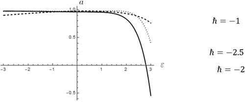
It is obvious from Figure 1 that $a\approx 1$ which agrees with the expected value and a valid region for ε is roughly between $-2/5$ and 2/5. For the rest of the paper and for all the values of b that have been taken into consideration, the value $ϵ=1/10$ will be used, since several simulations pointed out this value as reasonable.

After having fixed ε, the next step is to determine an appropriate value for ℏ. This was done by minimizing the errors defined by (44(44) $E_M\approx \frac{1}{N+1}\sum _{j=0}^N\left[\mathcal{N}\right(W_m\left({\eta }_j\right),a_M){]}^2,$(44) ). The second, third and fifth column of Table 1, show the optimum values for ℏ, the corresponding errors and the values of a in the case where b = 3, for several values of the order M from 8 up to 25. As the order increases, the error reduces as expected and a converges to the rounded value 0.974.

Table 1. $W_M^{\prime }\left(0^{+}\right),a_M,I_M$ and corresponding errors for $b=3,ϵ=1/10$ and the optimum ℏ.

Order M	ℏ optimum	Error $E_M$	$W_M^{\prime }\left(0^{+}\right)$	${\alpha }_M$	$I_M$
8	−1.617353369	8.449544572$\times {10}^{-7}$	−1.008493714	0.973736	1.999996348
9	−1.444432581	4.530287629$\times {10}^{-8}$	−1.009953643	0.973721	2.000013154
10	−1.305368461	4.378280872$\times {10}^{-11}$	−1.011095919	0.97371	1.999995500
15	−0.8827970199	7.718036623$\times {10}^{-9}$	−1.014312999	0.973679	2.000057168
17	−2.178369930	1.052302111$\times {10}^{-7}$	−1.015023210	0.973832	2.000134411
20	−0.6676018923	1.083197693$\times {10}^{-9}$	−1.015800585	0.973671	1.999779293
24	−1.668253179	6.404635995$\times {10}^{-16}$	−0.9730587006	0.973798	2.012913
25	−1.614707284	7.123265317$\times {10}^{-17}$	−0.9687500000	0.973798	2.031331769

As pointed out in Section 2.1, the first derivative of the peakon at the crest is not continuous and thus an initial condition on $w^{\prime }\left(0\right)$ cannot be utilized in the framework of HAM. This makes the estimation of $w^{\prime }\left(0^{+}\right)$ especially important. The Mth order approximation of $w^{\prime }\left(0^{+}\right)$ is given by the value of $W_M^{\prime }\left(0^{+}\right)$ depicted at the fourth column of Table 1, showing a very good agreement between the calculated by HAM value and the expected one.

Another important quantity is the integral $I={\int }_{\mathbb{R}}{u}^2+u_x^2$, i.e. the $H^1$ norm of the solution of (1(1) $u_t-u_{xxt}=u^2{u}_{xxx}+bu{u}_x{u}_{xx}-(b+1)u^2{u}_x,u=u(x,t),$(1) ), which is a conserved quantity as shown in [2,12]. This conserved quantity can be considered as conservation of energy for the peakon solution of (1(1) $u_t-u_{xxt}=u^2{u}_{xxx}+bu{u}_x{u}_{xx}-(b+1)u^2{u}_x,u=u(x,t),$(1) ). Since the peakon decays exponentially to zero, it suffices to calculate the integral $\tilde{I}={\int }_{-20}^{20}(u^2+u_x^2)dx$ instead of I. The Mth order approximation of $\tilde{I}$ is given by the value of $I_M$ depicted at the sixth column of Table 1, showing again a very good agreement between the calculated by HAM values and the expected ones.

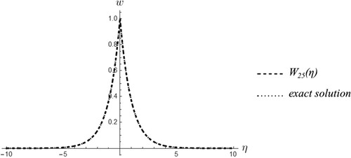
Moreover, in Figure 2 the ℏ-curve for a is given for the 25th order approximation of the solution. It is evident that the values for the optimum ℏ are in accordance with this ℏ-curve. The graph of the 25th order approximation of the solution via HAM for the corresponding optimum ℏ is given in Figure 3, against the graph of the exact solution (6(6) $\tilde{u}(x,t)=\sqrt{c}{e}^{-|x-ct|}.$(6) ) for c = 1. It is observed that there is an excellent agreement between the two.

Figure 2. ℏ-curve for a for 25 terms in the case $b=3,ϵ=1/10$.

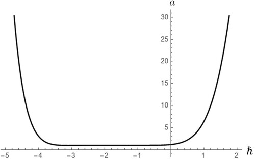
Figure 3. Comparison of the HAM solution in the case b = 3 for M = 25 with the exact solution for c = 1.

The same analysis has been carried out by the authors for various values of b, with results analogous to the obtained results for b = 3. Indicatively, tables similar to Table 1 are given for the values b = 4, b = 5 and b = 7 (see Tables 2–4). The results indicate that although HAM is successful in all four cases, the errors increase as b increases albeit they still remain small. This could possibly be overcome by changing ε or even $\mathcal{L}$.

Table 2. $W_M^{\prime }\left(0^{+}\right),a_M,I_M$ and corresponding errors for $b=4,ϵ=1/10$ and the optimum ℏ.

Order M	ℏ optimum	Error $E_M$	$W_M^{\prime }\left(0^{+}\right)$	${\alpha }_M$	$I_M$
8	0.2224414534	0.001025598693	−0.8843128928	1.22975	2.009428999
9	−2.093167808	5.053988212$\times {10}^{-7}$	−1.053522706	0.975303	2.002245310
12	0.1513458008	0.001140536645	−1.054005292	1.234840	2.002222841
15	−1.262094776	3.351849415$\times {10}^{-9}$	−1.054279739	0.975295	2.002209671
18	−1.054498366	3.775279136$\times {10}^{-10}$	−1.054456710	0.975288	2.002201011
20	−2.143279832	1.419991572$\times {10}^{-10}$	−1.029730319	0.975293	2.005545567
22	−1.971675913	4.030587317$\times {10}^{-13}$	−1.030694337	0.975293	2.033309664
25	−0.7626484933	3.856846270$\times {10}^{-11}$	−0.9999145242	0.975278	2.000000

Table 3. $W_M^{\prime }\left(0^{+}\right),a_M,I_M$ and corresponding errors for $b=5,ϵ=1/10$ and the optimum ℏ.

Order M	ℏ optimum	Error $E_M$	$W_M^{\prime }\left(0^{+}\right)$	${\alpha }_M$	$I_M$
8	0.2643960987	0.001094055946	−1.044673189	1.13628	2.001854527
10	0.6058643104	0.001379775954	−1.045096267	1.41501	2.001837876
12	0.1810971670	0.001223653884	−0.9419726231	1.14019	2.003916570
15	0.4097508998	0.0008456267111	−0.9450279818	1.43047	2.003661605
17	0.1300017376	0.001306487514	−0.946835635	1.14271	2.003498190
22	−1.024664469	2.074067836$\times {10}^{-8}$	−1.045894174	0.969545	2.001801420
25	−0.9036690081	2.258940949$\times {10}^{-8}$	−0.9520986085	0.969552	2.003014430

Table 4. $W_M^{\prime }\left(0^{+}\right),a_M,I_M$ and corresponding errors for $b=7,ϵ=1/10$ and the optimum ℏ.

Order M	ℏ optimum	Error $E_M$	$W_M^{\prime }\left(0^{+}\right)$	${\alpha }_M$	$I_M$
8	0.363427489	0.001228857332	−1.035050491	0.982103	2.001473782
10	0.2971040509	0.001328117791	−1.035411545	0.983408	2.001456406
12	0.6007517097	0.004309264124	−1.035612117	0.971101	2.001444318
15	0.2043253458	0.001472465928	−1.035780877	1.001360	2.001431777
17	0.1816863830	0.001508201948	−1.035849219	0.993373	2.001425705
20	0.3871955685	0.0009707760879	−0.9809711265	0.985117	2.001547175
22	0.3510259272	0.0007746105176	−0.9816103837	0.981237	2.001483956
25	0.3072731873	0.0006458985424	−0.9824790221	0.976949	2.00001

4. Conclusions

In this paper, the HAM was applied in order to analytically obtain several approximations of the peakon solutions to the b-Novikov Equation (1(1) $u_t-u_{xxt}=u^2{u}_{xxx}+bu{u}_x{u}_{xx}-(b+1)u^2{u}_x,u=u(x,t),$(1) ). Four values of b were taken into consideration, including b = 3 which corresponds to the well known Novikov equation. The obtained results are in excellent agreement with the exact ones.

This work complements earlier works of [20,21], where peakon solutions were studied in a similar way for the Degasperis-Processi and Camassa-Holm equations, which include quadratic nonlinearities. Since (1(1) $u_t-u_{xxt}=u^2{u}_{xxx}+bu{u}_x{u}_{xx}-(b+1)u^2{u}_x,u=u(x,t),$(1) ) is a special case of the more general Equation (3(3) $u_t-u_{xxt}=u^k{u}_{xxx}+b{u}^{k-1}{u}_x{u}_{xx}-(b+1)u^k{u}_x,u=u(x,t),$(3) ), HAM provides an excellent tool for further investigation of peakon solutions to not only (3(3) $u_t-u_{xxt}=u^k{u}_{xxx}+b{u}^{k-1}{u}_x{u}_{xx}-(b+1)u^k{u}_x,u=u(x,t),$(3) ), but also to other nonlinear PDEs.

Acknowledgments

The authors would like to thank the reviewers for their valuable comments which improved the presentation of the paper and also strengthened the reported findings.

Disclosure statement

The authors report that there are no competing interests to declare.

References

- Grayshan K, Himonas AA. Equations with peakon traveling wave solutions. Adv Dyn Syst Appl. 2013;8:217–232.
- Anco SC, da Silva PL, Freire IL. A family of wave-breaking equations generalizing the Camassa-Holm and Novikov equations. J Math Phys. 2015;56(9):Article ID 091506. 21.
- Novikov V. Generalizations of the Camassa-Holm equation. J Phys A. 2009;42(34):Article ID 342002.
- Efstathiou AG, Petropoulou EN. Peakons of Novikov equation via the homotopy analysis method. Symmetry. 2021;13(5):738.
- Himonas AA, Holliman C, Kenig C. Construction of 2-peakon solutions and ill-posedness for the Novikov equation. SIAM J Math Anal. 2018;50(3):2968–3006.
- Lundmark H, Shuaib B. Ghostpeakons and characteristic curves for the Camassa-Holm, Degasperis-Procesi and Novikov equations. SIGMA Symmetry Integrab Geom Methods Appl. 2019;15:017.
- Liu X, Liu Y, Qu C. Stability of peakons for the Novikov equation. J Math Pures Appl. 2014;101(2):172–187.
- Hone ANW, Lundmark H, Szmigielski J. Explicit multipeakon solutions of Novikov's cubically nonlinear integrable Camassa-Holm type equation. Dyn Partial Differ Equ. 2009;6(3):253–289.
- Mi Y, Mu C. On the Cauchy problem for the modified Novikov equation with peakon solutions. J Differ Equ. 2013;254(3):961–982.
- Zhou S, Chen R. A few remarks on the generalized Novikov equation. J Inequal Appl. 2013;2013(1):560.
- Himonas AA, Holliman C. Instability and nonuniqueness for the b-Novikov equation. J Nonlinear Sci. 2022;32(4), Paper 46 (29 pp). doi:10.1007/s00332-022-09798-6.
- da Silva PL, Freire IL. On the group analysis of a modified Novikov equation. In Cojocaru MG, Kotsireas IS, Makarov RN, et al. editors, Interdisciplinary topics in applied mathematics, modeling and computational science, Springer Proceedings in Mathematics & Statistics, Vol. 117. 2015. p. 161–166.
- Holm DD, Staley MF. Wave structure and nonlinear balances in a family of evolutionary PDEs. SIAM J Appl Dyn Syst. 2003;2(3):323–380.
- Holm DD, Staley MF. Nonlinear balance and exchange of stability in dynamics of solitons, peakons, rambs/cliffs and leftons in a 1−−1 nonlinear evolutionary PDE. Phys Lett A. 2003;308(5–6):437–444.
- Artebrand R, Schroll HJ. Numerical simulation of Camassa–Holm peakons by adaptive upwinding. Appl Numer Math. 2006;56(5):695–711.
- Kalisch H, Lenells J. Numerical study of traveling-wave solutions for the Camassa–Holm equation. Chaos Solitons Fract. 2005;25(2):287–298.
- Xu Y, Shu C-W. Local discontinuous Galerkin method for the Camassa–Holm equation. SIAM J Numer Anal. 2006;46(4):1998–2021.
- Liao SJ. Beyond perturbation: introduction to the homotopy analysis method. Boca Raton: Chapman & Hall/CRC, CRC Press LLC; 2004.
- Liao SJ. Homotopy analysis method in nonlinear differential equations. Heidelberg: Springer & Higher Education Press; 2012.
- Abbasbandy S, Parkes EJ. Solitary-wave solutions of the Degasperis–Procesi equation by means of the homotopy analysis method. Int J Comput Math. 2010;87(10):2303–2313.
- Wu W, Liao SJ. Solving solitary waves with discontinuity by means of the homotopy analysis method. Chaos Solitons Fract. 2005;26(1):177–185.
- Liao SJ. Chance and challenge: a brief review of homotopy analysis method. In Liao S, editor. Advances in the homotopy analysis method. Hackensack, NJ: World Sci. Publ.; 2014.