
 ?Mathematical formulae have been encoded as MathML and are displayed in this HTML version using MathJax in order to improve their display. Uncheck the box to turn MathJax off. This feature requires Javascript. Click on a formula to zoom.
ABSTRACT
Ethiopia is one of the countries highly affected by the COVID-19 pandemic in Africa. A new study has looked at the transmission dynamics of the outbreak in Ethiopia based on the age categories of the infected individuals. Infected individuals are divided into three age categories (less than 14 years (I), 15–54 years (I
), and above 54 years I
). Chebyshev polynomial of the fourth kind is used to convert a fractional system into an algebraic system of equations, which is then solved using iterative methods. The fundamental reproduction number
is calculated using the next-generation matrix technique, and the disease-free and endemic equilibrium points, as well as their stability, are carefully studied. We calculated the parameters and starting conditions provided for our model using data from the Ethiopian Public Health Institute (EPHI) and the Ethiopian Ministry of Health from 29 February 2021, to 7 June 2021.
1. Introduction and preliminary
Currently, Coronavirus disease 2019 (COVID-19) is a world health problem that has affected and killed millions of people. In December 2019, Wuhan, China, marked the beginning of a new Coronavirus outbreak [Citation1, Citation2]. On March 11, 2020, the World Health Organization (WHO) named the disease a pandemic [Citation3]. The most frequent symptoms are fever, dry cough, and shortness of breath, or trouble breathing. Symptoms include muscle and joint pain, headaches, sore throats, and a lack of taste or smell. To minimize this deadly disease from spreading further, social distance, face mask, washing hands frequently, minimizing non-essential trips, case isolation, family quarantine, and college and university closure are all being done [Citation4–9].
The Ethiopian Federal Ministry of Health (MOHE) and the Ethiopian Public Health Institute (EPHI) reported the first case of Covid-19 in Addis Ababa on March 13, 2020. The first case was a 48-year-old Japanese man who traveled from Japan to Burkina Faso before arriving in Addis Ababa [Citation10]. According to MOHE and EPHI's public health recommendations, anyone could be the next person to acquire COVID-19, but we can prevent it if we act immediately. We must use all COVID-19 intervention techniques to stay alive and well. Older people and those with pre-existing medical conditions (such as cardiovascular disease, chronic respiratory disease, or diabetes) are at high risk for severe disease.
In Ethiopia, there were 272, 914 confirmed COVID-19 cases and 4209 deaths as of June 6, 2021. This puts Ethiopia in fourth place in Africa in terms of confirmed cases and fifth place in terms of deaths caused by COVID-19. This week, there was a 27% decrease in the number of COVID-19 confirmed cases (for the ninth consecutive week), and there was a 32% decrease in the number of deaths due to COVID-19. The number of COVID-19 confirmed cases, deaths due to COVID-19, and laboratory tests and positivity rate in Ethiopia have shown a decrement in the last consecutive weeks [Citation11]. Habenom et al. [Citation12, Citation13] developed a fractionalized mathematical model for the Covid-19 epidemic's transmission in Ethiopia, which also helps analyse the Covid virus's behaviour.
In outbreak investigations, mathematical modeling is often utilized to understand the processes of infectious disease transmission and to interpret trends in epidemiological data [Citation14]. Agarwal et al. [Citation15] developed a mathematical model for transmission analysis based on the infection dynamics of the pandemic COVID-19. In which the basic reproduction number and balance points are calculated from the model to assess the transmittance of COVID-19. According to medical reports, both dengue and covid-19 have similar symptoms in the early stages. The transmission dynamics of both lethal viruses have been evaluated and predicted in co-infection modeling [Citation16].
Mathematical modeling has become a key tool in assessing the spread and management of infectious diseases, taking into consideration essential variables that influence disease progression, such as transmission and recovery rates. Models based on mathematics can be used to predict how the disease will spread over time [Citation17–19]. Based on the conservation principle of population dynamics, suitable mathematical models for COVID-19 pandemic outbreaks have been established [Citation20–22]. In [Citation23], to extend the Covid-19 model, a set of real-world data was used by taking into account the isolation and quarantine. Chowdhury et al. [Citation24] have analysed the interaction between the immune system and SARS-CoV-2 within the host. And also, Chowdhury et al. [Citation25] gave a mathematical model that deals with the asymptomatic and symptomatic disease transmission process in the COVID-19 outbreak. There has been a lot of interest in using mathematical models and simulations to explore the dynamics of infectious diseases in recent years [Citation26], because they help us better understand how diseases spread and provide a better understanding of epidemiological data. Essential parameters that may have a high influence on the outbreak rate and control strategies of Coronavirus disease 2019 are seen.
In a different way, Mahmoudi et al. [Citation27] studied the spread of COVID-19 in the United States, Spain, Italy, the United Kingdom, Germany, France, and Iran using the fuzzy clustering technique. Simultaneously, Din et al. [Citation28] investigated the stationary distribution of the pandemic COVID-19 and the extinction of the disease using stochastic methods. The computation of derivatives or integrals of any positive real order is considered as fractional calculus. Fractional calculus has attracted the interest of many researchers in different areas, including mathematics, physics, chemistry, biology, engineering, and even finance and social science, in recent years [Citation29–32]. In this paper, we investigated a mathematical model for COVID-19 that might be used to investigate Coronavirus transmission dynamics in Ethiopia based on the age categories of infected people. The dynamical transmission mechanism of the new Coronavirus is studied using Caputo fractional derivative.
The Mittag-Leffler (M-L) function, the fractional derivative, and a few key Chebyshev polynomial of the fourth type characteristics are covered in this section.
1.1. The Mittag-Leffler function
The one-parameter and two-parameter representations of the M-L function in terms of a power series are as follow [Citation33]:
(1)
(1)
and
(2)
(2)
where the function
, commonly referred to as Euler's integral, is defined as
(3)
(3)
From Ref. [Citation34], the Laplace transform of the function
is
(4)
(4)
1.2. Caputo fractional derivative
The fractional derivative of order δ in Caputo sense is defined in the following form Refs. [Citation35–37]
(5)
(5)
For Caputo fractional derivative, we have
(6)
(6)
(7)
(7)
where
and
denote the smallest integer greater than or equal to δ.
The Laplace transform of is given by:
(8)
(8)
with
is the Laplace transform of
.
1.3. Chebyshev polynomials of the fourth kind
On the interval , Chebyshev polynomials of fourth kind
can be generated using the following recurrence relation [Citation38]:
(9)
(9)
with starting polynomials
. Applying these polynomials on the interval
, we have the so-called shifted Chebyshev polynomials (SCP) of the fourth kind with the change of variable x = 2t−1. Let the SCP of the fourth kind
is denoted by
and it can be obtained as follows:
(10)
(10)
where
. The analytic form of
of degree n is given by:
(11)
(11)
A function
, square-integrable on
is represented by an infinite expansion of
as
(12)
(12)
The coefficients
are given by
(13)
(13)
The first
-- terms of shifted Chebyshev polynomials of the fourth kind are considered. Then we have
(14)
(14)
For suitable SCP of the fourth kind collocation method, we have to collocate Equation (Equation14
(14)
(14) ) at
shifted Chebyshev fourth kind roots
.
Lemma 1.1
Let be a function approximated in terms of the SCP fourth type provided in Equation (Equation14
(14)
(14) ), and suppose
, then
(15)
(15)
where is given by
(16)
(16)
2. Material and methods
The majority of confirmed cases admitted to treatment centres in Ethiopia were between the ages of 15 and 54, with the majority of COVID-19-related deaths occurring in those over 64 years old, according to reported cases. This means that as the patient gets older, the chances of dying from COVID-19 increase. We divide the total population of Ethiopia into seven different classes named as susceptible (S), exposed (E), and infected people are divided into three age groups (i.e. less than 14 years (I), 15–54 years (I
), and above 54 years (I
), hospitalized (H), and recovered and removed (R). The total population at any time t is given by
(17)
(17)
Individuals who have been recruited are assumed to be susceptible to a constant recruitment rate of Λ. Susceptible individuals get infected by infectious individuals with the force of infection
(Figure ).
Figure 1. Flow diagram of the SEII
I
HR model.
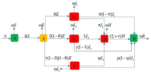
Figure 2. Confirmed cases and recovered cases from 29 February 2021 to 7 June 2021, in Ethiopia.
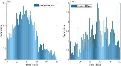
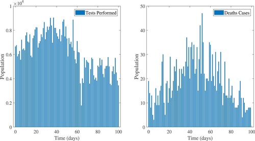
Figure 3. Testes performed and death cases from 29 February 2021 to 7 June 2021, in Ethiopia.
In the Caputo sense, the above model can be expressed as a system of fractional-order differential equations:
(18)
(18)
where,
with positive starting conditions
(19)
(19)
The parameter Λ is the recruitment rate, ω is the natural death rate, ℵ is the rate of transmission (or contact rate), ε is the modification factor for infected class I
, ϖ is the modification factor for infected class I
, θ is the rate of the exposed population joining the infected class I
, δ is the rate of the exposed population joining infected class I
, and τ is the rate of joining the infected class I
from the exposed The parameters π, λ, and ψ are rates at which infected individuals from I
, I
, and I
are in hospital (or treatment centre). σ, γ, and µ are recovery rates from I
, I
, and I
. ξ is the rate at which hospitalized individuals are recovered and ν is COVID-19-induced death rate. Because model (Equation18
(18)
(18) ) monitors the dynamics of the human population during the COVID-19 pandemic period, all the parameters are assumed to be non-negative.
2.1. Existence and uniqueness of solutions of SEI IIHR model
One of the most important fields in the theory of fractional-order differential equations is the theory of solution existence and uniqueness [Citation34, Citation39] and the references therein for some of the recent growth. Using the fixed point theorem [Citation40], we will discuss the existence and uniqueness of solutions to the proposed model in this section. We simplify the proposed model (Equation18(18)
(18) ) in the following setting:
(20)
(20)
where
(21)
(21)
Thus, the proposed model (Equation20
(20)
(20) ) has the form
(22)
(22)
under the condition that
(23)
(23)
Problem (Equation22
(22)
(22) ) which is equivalent to model (Equation18
(18)
(18) ) has an integral representation is given by
(24)
(24)
Let
stand for the Banach space of all continuous functions from
to
with the norm defined by
(25)
(25)
where
and
.
Theorem 2.1
For every kernels
in (Equation21
(21)
(21) ), there exist
such that
(26)
(26)
where y is the state vector presented as and are contractions for
Proof.
For the state variable S, we have
where
,
It then follows that
satisfies the Lipschitz condition with Lipschitz constant
. Moreover, if
, then
is a contraction. In the same way, we can show the existence of Lipschitz constants
and a contraction principle for
. Now for
defined the following recursive form of (Equation24
(24)
(24) )
(27)
(27)
The difference between successive terms in the above equation and taking the norm on both sides of the resulting equation, we obtain:
(28)
(28)
Furthermore, by taking y = S Equation (Equation28
(28)
(28) ) can be reduced to the following expressions:
As a result, we have
(29)
(29)
The rest of the expressions can be reduced to the following form:
(30)
(30)
Theorem 2.2
The Caputo fractional model given in (Equation18(18)
(18) ) has a solution if we can find ℑ satisfying the inequality
(31)
(31)
Proof.
From (Equation29(29)
(29) ) and (Equation30
(30)
(30) ) we have
(32)
(32)
Theorem 2.1 confirmed the existence of solution, and we have to show that the functions
are solutions of model (Equation18
(18)
(18) ).
Let us assume that the following are satisfied:
(33)
(33)
From (Equation33
(33)
(33) ) we obtain
(34)
(34)
Recursively repeating the process results in
(35)
(35)
Taking
yields
(36)
(36)
Applying the limit to both sides of (Equation36
(36)
(36) ) as
we see that
for
Theorems 2.1 and 2.2 guarantees the existence of the solution of model (Equation18
(18)
(18) ) by the Banach fixed point theorem [Citation41].
Theorem 2.3
uniqueness of solutions
The Caputo fractional model (Equation18(18)
(18) ) has a unique solution provided that
(37)
(37)
Proof.
Let us assume that are solutions to (Equation18
(18)
(18) ). Then
(38)
(38)
Taking the norm of both sides, obtain
(39)
(39)
Since
we obtain
. Thus, we have
.
In the same way, we can show that
.
Lemma 2.1
The epidemiologically feasible region of model (Equation18(18)
(18) ) is given by
(40)
(40)
with positive initial conditions in (Equation19
(19)
(19) ) is a positive invariant for system (Equation18
(18)
(18) ).
Proof.
Adding each equation in model (Equation18(18)
(18) ) yields the dynamics of the overall population, given by
(41)
(41)
Applying the Laplace transform on (Equation41
(41)
(41) ) and the idea of (Equation4
(4)
(4) ), we obtain:
(42)
(42)
Since,
we have
and hence, the region Θ is a positively invariant set for the system (Equation18
(18)
(18) ).
Theorem 2.4
If the starting solutions satisfy
, then the solutions
,
of the system (Equation18
(18)
(18) ) are positive
.
Proof.
Take the first equation of the COVID-19 model (Equation18(18)
(18) )
(43)
(43)
where
.
Following Lemma 2.1, which is bounded by a constant
, we have
(44)
(44)
where r is a constant equal to
Applying the Laplace transform in the previous inequality (Equation44(44)
(44) ), we arrive at
(45)
(45)
Since
and
, then the solution
is positive. Similarly, it can be shown that the quantities (
,
) are positive
.
2.2. Stability analysis of SEIIIHR model
The disease-free equilibrium corresponds to the case when there are no infections in the population. All the infectious compartments are set to zero. That is . Also, setting the fractional derivatives of non-infectious compartments to zero in our model equation (Equation18
(18)
(18) ). That is
. Hence, the disease-free equilibrium point
is given by
(46)
(46)
The matrix S at
given by
and the matrix T at
is
Then, the largest eigenvalue of the next generation matrix
is the required effective reproduction number which is given by
(47)
(47)
Three effective reproduction numbers are comprised in Equation (Equation47
(47)
(47) ). The first number is
, it is defined as the number of new COVID-19 cases generated from the first age class of infected individuals (I
), the second number is
defined as the number of cases generated from the second age class of infected individuals (I
) and the third number is
, and it defines the number of COVID-19 cases generated from the third-age class of infected individuals (I
). It can be written as a mathematical expression:
(48)
(48)
Theorem 2.5
If , then the disease-free equilibrium point
in Equation (Equation46
(46)
(46) ) is locally asymptotically stable and unstable for
.
Proof.
To assess the local stability of the disease-free equilibrium point, we investigate the behaviour of our model population near this equilibrium solution. At , the Jacobian matrix of (Equation18
(18)
(18) ) is now:
(49)
(49)
The three eigenvalues are negative. i.e.
and the following characteristic equation can be used to find the remaining eigenvalues.
where
In the above expressions, the coefficients
,
and
are positive when
, and the coefficient
is positive. Further, the Routh-Hurwitz criteria for fourth-order polynomials are
,
can be easily satisfied by using the coefficients listed above. So, the model (Equation18
(18)
(18) ) at
is locally asymptotically stable if
and unstable if
We equate system (Equation18(18)
(18) ) to zero and solve simultaneously to identify an infectious equilibrium point. Thus, the endemic equilibrium is
and
which satisfy the quadratic equation
Only for
does a positive endemic equilibrium point exist, whereas for
, no endemic equilibrium exists.
Theorem 2.6
If , then the disease-free equilibrium point
in Equation (Equation46
(46)
(46) ) is globally asymptotically stable on a positively invariant region Θ.
Proof.
Consider the Lyapunov function:
(50)
(50)
Differentiate the Lyapunov function
at a time t in Caputo fractional derivative, we obtain
(51)
(51)
Substituting appropriate value from the model Equation (Equation18
(18)
(18) )
As
and
,
Choose,
There are no negative model parameters; it follows that
for
and
if and only if, E = 0. As a result, if
,
is globally asymptotically stable in a positively invariant region Θ, according to LaSalle's invariance principle.
2.3. The Chebyshev spectral collocation method for the solutions of SEIIIHR model
Consider the fractional SEII
I
HR model of COVID-19 of the type given in Equation (Equation18
(18)
(18) ). To apply the shifted Chebyshev polynomials of the fourth type collocation method, we first approximate
,
,
and
in terms of these polynomials with m = 3 and
as:
(52)
(52)
Now, using the concept of Lemma 1.1 and Equation (Equation52
(52)
(52) ) on the model Equation (Equation18
(18)
(18) ), we obtaine:
We use roots of shifted Chebyshev polynomial
for suitable collocation points. Also, by substituting Equation (Equation52
(52)
(52) ) in the positive initial conditions (Equation19
(19)
(19) ), we can obtain seven equations
(53)
(53)
Then, we have 28 equations that can be solved using inexact Newton's method, for the unknowns
and
for
.
3. Result and discussion
3.1. Numerical simulation
Numerical solutions for the model SEII
I
HR is made based on the real data of COVID-19 confirmed cases of Ethiopia for 101 days from 29 February 2021 to 7 June 2021 [Citation11]. Ethiopia's total population is approximately
, with a life expectancy of 67.8 years in 2021. As a result, the natural death rate is calculated as
. Further, from 5724 tests performed on 29 February 2021, in Ethiopia 935 new confirmed COVID-19 cases were reported. Of these, 33 were infected cases in age 0-14 years (3.12 % of the newly confirmed cases), 703 were infected cases in age 15–54 years (71.9% of the newly confirmed cases), and the remaining 199 were infected cases in age greater than 54 years. On this day, there were 954 newly recovered COVID-19 cases and 20,144 active cases (cases on treatments). The initial population is assumed
. The parameter Λ is calculated from the relation
per day.
A numerical simulation will be performed based on the reported cases in Ethiopia, with the following initial conditions for the system (Equation18(18)
(18) ):
Sensitivity analysis of
: Sensitivity analysis is important for identifying parameters that can be targeted in designing control strategies. The index measures the relative change in
with respect to the relative change in the parameters [Citation42, Citation43]. Based on the epidemiological parameters in Table , we performed the sensitivity of the basic reproduction number
. Changes in
are associated with changes in different parameters of the model (Equation18
(18)
(18) ) at their given values in this analysis.
The sensitivity of with respect to a model parameter r is given by
(54)
(54)
Table 1. Best fitted, assumed and calculated parameters used in model (Equation18(18)
(18) ).
From Table , the most sensitive parameters are the transmission rate (ℵ), the contact rate from the infected people in age 15–54 years to the susceptible people (ε), the rate of hospitalization for the infected cases in age 15–54 years (λ), the contact rate from the infected people in age greater than 54 years to the susceptible people (ϖ), and the rate of hospitalization for the infected cases in age greater than 54 years (ψ). These parameters have a significant effect on the value of the basic reproduction number . Decreasing the rate of transmission ℵ gives a reduction in the value of the basic reproduction number
. It would be very effective in reducing the basic reproduction number if the virus's transmission in the population could be controlled. Similarly, decreasing the parameters ε, ϖ, δ and θ which are the contact rate from infected cases age 15–54 years to the susceptible population, the contact rate from the infected cases age above 54 years to the susceptible population, the rate of progression from exposed to infected group age 15–54 years, the rate of progression from exposed to the infected group age less than 14 years, respectively, lead to the decrease in the value of the basic reproduction number
. Also, increasing the values of the parameters λ, ψ, and π which are the rate of hospitalization for infected cases age 15–54 years, above 54 years, and less than 14 years, respectively, lead to the decreasing on the value of the basic reproduction number
. The best strategies for controlling the pandemic are to reduce the rate of transmission in the population and to improve the treatment of patients in treatment centres. When all other parameters are kept constant, the value of each parameter that gives a stable reproduction number (
) is as follows:
Other parameters change within their suitable range, making all their own effects, even the value of the reproduction number greater than or less than one.
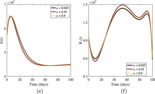
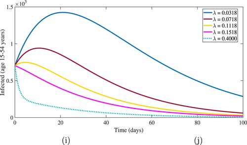
The graphical interpretations of Figures and show the behaviour of our numerical results for susceptible and infected population based on different values of .
Figure 4. Numerical results of I and I
for different values of
.
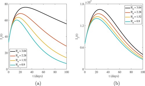
Figure 5. For various values of , numerical results of
and I
.
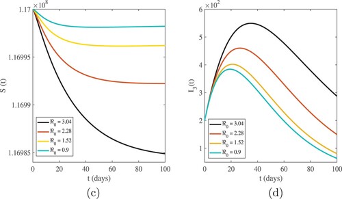
Table 2. Sensitivity of the basic reproduction number with respect to epidemiological parameters in Table .
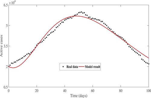
In Figures and , we compared the SEII
I
HR model results to the EPHI data of daily reported cases in all age groups and daily active cases for the 2019 Coronavirus disease in Ethiopia. The simulated results are very close to actual data on infected and active cases obtained from the Ethiopia Ministry of Health and the Ethiopia Public Health Institute daily report for a 101-day period starting 29 February 2021.
Figure 6. In Ethiopia, real data and model results for daily infected cases between 29 February 2021 and 7 June 2021.
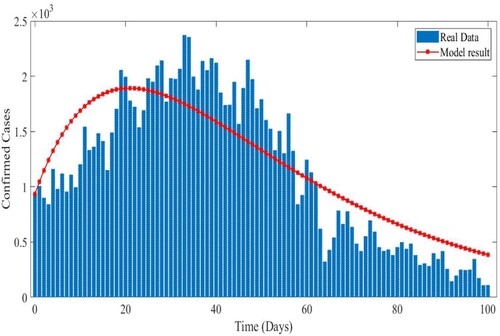
Figure 7. Real data and model result for daily active cases between 29 February 2021 and 7 June 2021.
The influence of fractional-order α on numerical solutions of the model compartments is shown in the graphical interpretations of Figures –.
Figure 8. Approximate solutions of I and I
for different α.
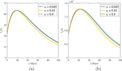
Figure 9. Approximate solutions of I and
for different α.
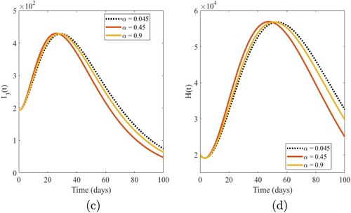
Figure 10. Approximate solutions of and
for different α.
3.2. Discussion
The reported data for confirmed, recovered, tests performed, and death cases in Ethiopia are shown in Figures and . In Equation (Equation18(18)
(18) ), Table provides the fitted, computed, and assumed parameters of a model. The fitted parameters were generated using least square curve fitting in MATLAB R2020a and real data was made available in Ref. [Citation11]. Table also discusses the sensitivity of the basic reproduction number
, and it is concluded that the transmission rate ℵ is the most sensitive parameter. This parameter influences
in a positive way. That is, decreasing transmission rate values results in decreasing
values. Keeping the other values in Table unchanged and reducing the transmission rate from 0.8896 to 0.1896,
reduces from 1.3545 to 0.2887. In addition, hospitalization rates for each age group of infected individuals have a negative impact on
. In other words, increasing the values of these parameters lowers the quantity of
. Figures and show that the highest value of the basic reproduction number
shows the highest number of cases in all age categories, and as the number of infected cases increases, the susceptible population decreases. For
, we have evidence that in this simulation, most of the susceptible individuals are rapidly decreasing and the infected cases are increasing. This indicates that one infected person will cause more than three new infections, and virus transmission will become uncontrollable. When the basic reproduction number
is used, the curves reveal that susceptible people increase and converge to the population's initial number, while infected individuals tend to be few. This indicates that the number of newly infected individuals is decreasing, that society is safe from the virus, and that the infection will eventually die out in the country. The comparison of real data and model findings for daily confirmed cases and active cases in Ethiopia is shown in Figures and . The reader may see from these illustrations that mathematical models have a lot of strength when it comes to expressing real-world problems. Figures and illustrate how lowering the transmission rate of the coronavirus due to infected cases in all age groups can help to slow the disease's progress. The basic reproduction number
will be reduced from 1.3545 to 0.9991 by decreasing the transmission rate from 0.8896 to 0.6562 per day. As a result, when
, a stable disease-free equilibrium is obtained. Figure shows how increasing the rate of hospitalization for infected cases (age 15–54 years) reduces the number of infected cases by a significant amount. When
,
and
, the corresponding basic reproduction number
,
and 0.8404, respectively. For the real data of COVID-19 cases in Ethiopia, the parameters in Table produced a value of the basic reproduction number
, which exceeds unity. This number indicates that the disease-free equilibrium point for model Equation (Equation18
(18)
(18) ) is locally asymptotically unstable, whereas the infectious equilibrium point is stable, implying that the coronavirus will persist in the population, as evidenced by the infectious population remaining positive in this numerical simulation. The transmission from infected cases aged below 14 years is
, which contributes 20.43% of the basic reproduction number, the transmission from infected cases age 15-54 years,
contributes the largest value 54.79% of the basic reproduction number and the transmission from infected cases aged greater than 54 years
, which contributes 24.78%. To control the spread of this virus in Ethiopia, managing transmission from infected cases in the age group of 15–54 years is pivotal and the Ethiopian government and all the responsible bodies should focus on transmission due to infected cases in the age group of 15–54 years.
Figure 11. Decreasing the transmission rate on the approximate solutions of E(t) and I at
.
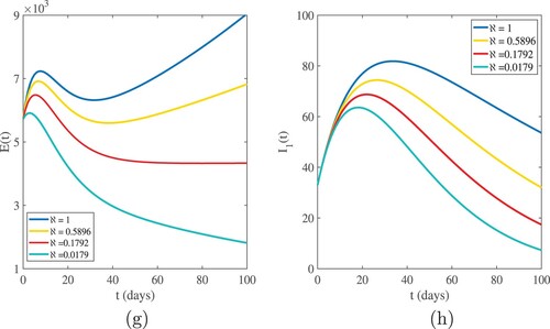
Figure 12. Decreasing the transmission rate on the approximate solutions of I and I
at
.
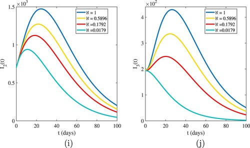
Figure 13. Increasing the hospitalization rate on the approximate solution of I at
.
4. Conclusion
In this paper, we have investigated the spread of COVID-19 disease using SEII
I
HR model and in the Caputo sense the model is presented as a system of fractional-order differential equations, with the numerical solutions achieved using the Chebyshev polynomials of the fourth kind. The proposed model is converted to a nonlinear system of algebraic equations that are solved using Newton's iteration method using the properties of this polynomial. The findings of the proposed model are found to be very close to the real data. The identification of key parameters that have a huge effect on basic reproduction number is important for creating the most effective and efficient disease prevention methods. The value of the basic reproductive number
shows that one COVID-19 tested positive person is the cause of more than one new infected individual. Therefore, the coronavirus spread is going on. As a result, we recommended everybody who is responsible for fully participating in reducing the value of the basic reproductive number to less than unity. The transmission rate plays a significant role in reducing the basic reproduction number, according to the simulated results in this work. For disease control, reducing virus transmission in the population is critical. Throughout the pandemic, the Ethiopian government must take the necessary steps to control strategy toward reducing
through sensitive parameters.
Disclosure statement
No potential conflict of interest was reported by the author(s).
Data availability statement
Data from COVID-19 cases in Ethiopia from 29 February 2021 to 7 June 2021 were utilized to support this investigation.
References
- Zhu H, Wei L, Niu P. The novel coronavirus outbreak in Wuhan. China: Global Health Research Policy; 2020. vol. 5, no. 6.
- Centers for Disease Control and Prevention, Outbreak of 2019 Novel Coronavirus (2019-nCoV) in Wuhan. 2020 Jan 21. Available from: www.cdc.gov/csels/dls/locs.
- World Health Organization, WHO characterizes Covid-19 as a pandemic. 2020 Mar 11. Available from: https://www.who.int/emergencies/diseases/novel-coronavirus-2019/situation-reports.
- World Health Organization (WHO), Advice for Public., Archived from the original on 2020 Jan 26. cited 2020 Feb 10.
- U. S. Centers for Disease Control and Prevention (CDC), Coronavirus Disease 2019 (COVID-19): Prevention and Treatment, Archived from the original on 2020 Mar 11. cited 2020 Mar 11.
- Mwalili S, Kimathi M, Ojiambo V, et al. SEIR Model for COVID-19 dynamics incorporating the environment and social distancing. Mwalili et al., editors. BMC Notes. Vol. 13, no. 352, Nairobi, Kenya: 2020 Apr.
- Moore SE, Okyere E. Controlling the Transmission Dynamics of COVID-19. Vol. 1, no. 1, University of Cape Coast; 2020 Mar. p. 13–21.
- Zeb A, Alzahrani E, Erturk VS, et al. Mathematical model for coronavirus disease 2019 (COVID-19) containing isolation class. London, United Kingdom: BioMed research international; 2020.
- Mishra AM, Purohit SD, Owolabi KM, et al. A nonlinear epidemiological model considering asymptotic and quarantine classes for SARS CoV-2 virus. Chaos Solitons Fractals. 2020;138:109953.
- World Health Organization, Ethiopia, the first case of COVID-19 confirmed in Ethiopia. 2020 Mar 13. Available from: https://www.afro.who.int/news/first-Marchcase-covid-19-confirmed-ethiopia.
- Ministry of Health-Ethiopia and Ethiopian Public Health Institute. 2021 Jun 6. Available from: www.moh.gov.et and http://www.ephi.gov.et/.
- Suthar DL, Habenom H, Aychluh M. Effect of vaccination on the transmission dynamics of COVID-19 in Ethiopia. Results Phys. 2022;32:105022. doi: 10.1016/j.rinp.2021.105022
- Habenom H, Aychluh M, Suthar DL, et al. Modeling and analysis on the transmission of covid-19 pandemic in Ethiopia. Alex Eng J. 2022;61(7):5323–5342.
- Brauer F. Mathematical epidemiology: past, present, and future. Infect Dis Model. 2017;2(2):113–127.
- Agarwal P, Ramadan MA, Rageh AA, et al. A fractional-order mathematical model for analyzing the pandemic trend of COVID-19. Math Methods Appl Sci. 2022;45(8):4625–4642.
- ul Rehman A, Singh R, Agarwal P. Modeling, analysis and prediction of new variants of covid-19 and dengue co-infection on complex network. Chaos Solitons Fractals. 2021;150:111008.
- Sahu GP, Dhar J. Dynamics of a SEQIHRS epidemic model with media coverage, quarantine, and isolation in a community with pre-existing immunity. J Math Anal Appl. 2015;421(2):1651–1672.
- Kermack WO, McKendrick AG. A contribution to the mathematical theory of epidemics. Proc R Soc A. 1927;115(772):700–721.
- Arafa AAM, Rida SZ, Khalil M. Solutions of fractional order model of childhood diseases with constant vaccination strategy. Math Sci Lett. 2012;1(1):17–23.
- Khan MA, Atangana A, Alzahrani E, et al. The dynamics of COVID-19 with quarantined and isolation. Adv Differ Equ. 2020;425:1–22.
- Naik PA, Yavuz M, Qureshi S, et al. Modeling and analysis of COVID-19 epidemics with treatment in fractional derivatives using real data from Pakistan. Eur Phys J Plus. 2020;135(795):1–42.
- Ahmad S, Ullah A, Al-Msallal QM, et al. Fractional order mathematical modeling of COVID-19 transmission. Nat C Biotech Info US Nat Lib Med. 2020;139:110256.
- Baleanu D, Abadi MH, Jajarmi A, et al. A new comparative study on the general fractional model of COVID-19 with isolation and quarantine effects. Alex Eng J. 2022;61(6):4779–4791.
- K. Chowdhury SME, Chowdhury JT, Ahmed SF, et al. Mathematical modelling of COVID-19 disease dynamics: interaction between immune system and SARS-CoV-2 within host. AIMS Math. 2022;7(2):2618–2633.
- K. Chowdhury SME, Forkan M, Ahmed SF, et al. Modeling the SARS-CoV-2 parallel transmission dynamics: asymptomatic and symptomatic pathways. Comput Biol Med. 2022;143105264.
- Gumel AB, Iboi EA, Ngonghala CN, et al. A primer on using mathematics to understand COVID-19 dynamics: modeling, analysis and simulations. Infect Dis Model. 2021;6:148–168.
- Mahmoudi MR, Baleanu D, Mansor Z, et al. Fuzzy clustering method to compare the spread rate of Covid-19 in the high risks countries. Chaos Solitons Fractals. 2020;140:110230.
- Din A, Khan A, Baleanu D. Stationary distribution and extinction of stochastic coronavirus (COVID-19) epidemic model. Chaos Solitons Fractals. 2020;139:110036.
- Podlubny I. Fractional differential equations: an introduction to fractional derivatives, fractional differential equations, to methods of their solution and some of their applications. Amsterdam, Netherlands: Elsevier; 1998.
- Baleanu D, Diethelm K, Scalas E, et al. Fractional calculus: models and numerical methods. Vol. 3. Singapore: World Scientific; 2012.
- Sun H, Zhang Y, Baleanu D, et al. A new collection of real world applications of fractional calculus in science and engineering. Commun Nonlinear Sci Numer Simul. 2018;64:213–231.
- Kiryakova V, Mainardi F, Machado JAT. Recent history of fractional calculus. Commun Nonlinear Sci Numer Simul. 2011;16(3):1140–1153.
- Abdo MS, Shah K, Wahash HA, et al. On a comprehensive model of the novel coronavirus (COVID-19) under Mittag-Leffler derivative. Chaos Solitons Fractals. 2020;135:109867.
- Khan A, Gomez-Aguilar J, Abdeljawad T, et al. Stability and numerical simulation of fractional order plant-nectar-pollinator model. Alex Eng J. 2020;59(1):49–59.
- Sontakke BR, Shaikh AS. Properties of Caputo operator and its applications to linear fractional differential equations. Int J Eng Res Appl. 2015;5(5):22–27.
- Kilbas AA, Srivastava HM, Trujillo JJ. Theory and applications of fractional differential equations. Amsterdam, Netherlands: Elsevier; 2006.
- Oldham KB, Spanier J. The fractional calculus. Cambridge, MA: Academic Press; 1974.
- Canuto C, Hussaini MY, Quarteroni A, et al. Spectral methods: fundamentals in single domain. Berlin, Germany: Springer; 2006.
- Khan H, Abdeljawad T, Aslam M, et al. Existence of positive solution and Hyres-Ulam stability for a nonlinear singular-delay-fractional differential equation. Adv Differ Equ. 2019;2019(104):1–13.
- Kirk WA, Vasile I. Fixed point theory: an introduction to metric spaces and fixed point theory. Hoboken, NJ: John Wiley; ISBN 0-471-41825-0.
- Pascal H, Seda AK. A 'Converse' of the Banach contraction mapping theorem. J Electr Eng. 2001;52:3–6.
- Nakul C, Hyman JM, Cushing JM. Determining important parameters in the spread of malaria through the sensitivity analysis of a mathematical model. Bull Math Biol. 2008;70(5):1272–1296.
- Okosun KO, Rachid O, Marcus N. Optimal control strategies and cost-effectiveness analysis of a malaria model. Biosystems. 2013;111(2):83–101.