Atangana–Baleanu derivative-based fractional model of COVID-19 dynamics in Ethiopia

ABSTRACT

The paper's main aim is to investigate the 2019 coronavirus disease in Ethiopia using a fractional-order mathematical model. It would also focus on the importance of fractional-order derivatives that may help us in modelling the system and understanding the effect of model parameters and fractional derivative orders on the approximate solutions of our model. A SELAIQHCR model is constructed using nonlinear differential equations in the Atangana–Baleanu non-integer operator in the Caputo sense. After that, the Chebyshev fourth kind spectral collocation method is used to change a fractional system to an algebraic system. Newton iterative technique is used to solve the converted system. The next-generation matrix technique is used to obtain the effective reproduction number. The COVID-19-free equilibrium point and endemic equilibrium point, solution positivity and boundedness, and their stability are all carefully done. The sensitivity of the effective reproduction value with respect to the key model parameters is discussed. The beginning values provided for our system were obtained using reports from the Ethiopian Public Health Institute from 29 February 2021 to 7 June 2021. The fundamental reproduction number is obtained with ${\mathfrak{R}}_0=1.4331$. The model's numerical solutions are represented graphically.

KEYWORDS:

• COVID-19
• Atangana–Baleanu fractional derivative
• stability analysis
• Chebyshev polynomials of fourth kind
• Chebyshev spectral collocation method

2010 MATHEMATICS SUBJECT CLASSIFICATIONS:

• 03C45
• 65M70
• 41A50
• 35C11

1. Introduction

In Wuhan, China, a fresh coronavirus infection began in December 2019 [1]. The disease was named a pandemic by the World Health Organization (WHO) on 11 March 2020 [2]. COVID-19 symptoms include fever, cough, headache, tiredness, and breathing difficulties. Physical distancing, face masks, hand washing, minimizing non-essential trips, lockdown of exposed cases, and school closures are all being used to slow the spread of this highly contagious disease [3–5]. Prevention of coronavirus disease in Ethiopia is difficult for a variety of reasons. Among them are the difficulties of screening infectious people, social problems, insufficient human power in treatment centres, less public awareness and the Ethiopian lifestyle [6]. These factors allow infectious and non-infectious individuals to interact.

Mathematical models are important tools for understanding outbreak dynamics. Mathematical models can be used to predict the future spread of the virus, helping the government to be prepared and take the required actions [7]. In epidemiology, compartmental dynamic models are a set of ordinary differential equations and parameters that track the temporal evolution of the number of people in each phase of the system. To understand the behaviour of coronavirus disease better, several mathematical models were created. By taking into account the impacts of isolation and quarantine, researchers in Ref. [8] investigated a new fractional model of COVID-19. The power-law, Mittag-Leffler, and exponential kernels were used to simulate the suggested model. The population was divided into four subgroups in Ref. [9]: Susceptible-Asymptomatic-Symptomatic-Recovered/Removed during the Coronavirus pandemic. A stochastic COVID-19 epidemic model with time delay was explored for its extinction and stationary distribution in Ref. [10]. They calculated the basic reproduction number under a stochastic model. Authors in Ref. [11] focused on the most effective tactics, controls, and techniques for effectively reducing coronavirus epidemics in Saudi Arabia. Susceptible, exposed, infected, quarantined, and recovered were the five essential dynamic sub-populations or categories that divided Saudi Arabia's population. They used real data from the Saudi Arabian COVID-19 outbreak report. They discovered a coronavirus-free equilibrium point that is unstable (${\mathfrak{R}}_0>1$). In other words, the rate at which a susceptible individual becomes exposed is more than one, indicating that COVID-19 transmission in Saudi Arabia is unstable. They advised the public to stay at home as much as possible to limit the progress of the coronavirus and send sick people to a safe place. They also came to the conclusion that preventing rather than recovering is preferable. Authors in Ref. [12], proposed the SEIR model, which included the environment and social distancing, was used to study COVID-19 dynamics. The authors used the RK4 and RK5 methods to approximate the solutions of a system. In Ref. [13], the authors looked at fractional derivatives, mathematical modelling, and the dynamics of the newly discovered virus in Wuhan, China. They started with the integer-order derivative and then applied the Atangana–Baleanu derivative to construct the model. They assumed that the transmission occurred within the bat population before it spread to the hosts. They used the least square curve fitting technique to fit or estimate the parameters from Wuhan, China, and they used values from the literature. In Ref. [14], the Caputo fractional-order model for COVID-19 with lockdown was used to study the importance of lockdown in preventing the transmission of the new virus. They addressed the model's existence and uniqueness using the fixed point theorem. Stability analysis was established in the Ulam–Hyers and generalized Ulam–Hyers frameworks. The fractional form of the model under discussion via the Caputo fractional operator has been numerically simulated. To display the profiles of each variable, they used Caputo's fractional derivative with the fractional-order value of $\nu =0.67$. With various fractional-order values, the illustrative and dynamical outlook of each variable were studied. Fractional mathematical models were used to study the dynamics of several infectious and noninfectious diseases, not alone COVID-19. For example, for a real data, authors in Refs. [15,16] created brand-new mathematical modelling of Tumor-Immune system using the generalized form of fractional derivative. A numerical scheme for solving their model is obtained using the product-integration rule. Various numerical simulations were done for different kernels and fractional orders. Moore et al. [17] used the Caputo–Fabrizio fractional derivative with an exponential decay kernel to construct a new HIV/AIDS epidemic with an antiretroviral treatment compartment.

The computation of derivatives or integrals of any positive real order is considered fractional calculus. The use of fractional differential equations has received a lot of attention in recent years. Many investigators use fractional differential equations in their field of study. For example, in Ref. [18], R. T. Alqahtani used fractional differential equations in his paper published in the journal of nonlinear science and applications. Deressa and Duressa looked at a SEAIR epidemic mathematical model that included the Atangana– Baleanu fractional derivative in Ref. [19]. More work on fractional differential equations can be obtained in Refs. [20–22] and the references therein. An exponential decay law-based derivative was proposed by Caputo and Fabrizio. This derivative has some advantages over previous definitions, including the ability to be used while observing the exponential law in nature and the absence of singularity because the kernel is built on an exponential function. However, there were very serious challenges made against this new discovery. First, the kernel used was not non-local; second, the anti-derivative associated is just the average of the function and its integral. As a result, it was determined that the operator was actually more of a filter than a fractional derivative. However, it is important to note that numerous successful activities have been carried out in the area of this recent finding [23–30]. Another crucial point was made by Atangana and Koca in their paper that was published in Chaos Soliton and Fractals, where they claimed that the solution to the equation ${}_0^{CF}{D}_t^{\gamma }\psi \left(t\right)=\psi \left(t\right)$ was an exponential function rather than a special function. To address the difficulties raised by Caputo–Fabrizio, Atangana and Baleanu proposed a significantly improved derivative with no singular kernel.. They have built their derivative on the well-known generalized Mittag-Leffler function. The significance of the Mittag-Leffler function was re-discovered while its relationship to fractional calculus was completely comprehended. Due to the impact of this function on modelling problems, we apply the Atangana–Baleanu fractional derivatives in the Caputo sense (ABC derivative) to the model of COVID-19.

The key benefit of spectral methods is their accuracy for a given set of unknowns. In many studies, spectral collocation techniques are used. In 2015 [31], using the Haar wavelet collocation method, numerical solutions to problems with singular initial values were discovered. The Haar wavelet collocation method is a numerical approach for solving integral equations, ordinary and partial equations in both integer and non-integer derivatives. To analyse the model of giving up smoking in fractional order, the authors in Ref. [32] provided a Chebyshev spectral approach. An approximate formula for the Caputo fractional derivative was derived using the properties of the Chebyshev polynomials. The formula reduced the model of giving up smoking to the solution of a system of algebraic equations, which was solved using the Newton iteration method. Motivated by recent works on spectral collocation methods for solving systems of equations, we apply the fourth kind of shifted Chebyshev spectral collocation method to the system of the fractional model of COVID-19.

The main purpose of this paper is to build a mathematical model for understanding COVID-19 transmission dynamics by utilizing real pandemic cases in Ethiopia with the aid of epidemiological modelling. Our motivation comes from several recently completed research works [33–40] in the literature that are based on deterministic modelling of coronavirus diseases in different nations. Compartmental modelling is used in each of these studies. The results of this study may support governments and public health officials in developing strategic action to limit the virus's spread and prevent any future outbreaks. There are so many studies that are related to this mathematical modelling that the proposed model can be seen as an important addition by increasing the interest among researchers that study fractional modelling.

The structure of this paper is as follows: In Section 2, we review some key information regarding the Mittag-Leffler function, fractional calculus in ABC definitions, and some fundamental points concerning fourth-kind Chebyshev polynomials. We will discuss the COVID-19 dynamical model in Section 3. Stability analysis, solution positivity, and the fundamental reproduction number are all covered in this section. In Section 4, we used the Chebyshev spectral collocation method to convert the fractional system into an algebraic system of equations. We present numerical approaches for the ABC derivative and give various graphical results for the fractional-order parameter γ. A discussion and conclusion are written at the end.

2. Preliminaries

2.1. Mittag-Leffler function

The M-L function is a direct generalization of $e^x$ that is widely used in fractional calculus.

Definition 2.1

The one parameter and two parameters representations of the M-L function in terms of the power series are as follows [41]: (1) $E_a\left(w\right)=\sum _{m=0}^{\mathrm{\infty }}\frac{w^m}{\mathrm{\Gamma }(am+1)},a>0,$(1) and (2) $E_{a,b}\left(w\right)=\sum _{m=0}^{\mathrm{\infty }}\frac{w^m}{\mathrm{\Gamma }(am+b)},a>0,b>0.$(2) where the function $\mathrm{\Gamma }\left(w\right)$ is defined as $\mathrm{\Gamma }\left(w\right)={\int }_0^{\mathrm{\infty }}{u}^{w-1}{e}^{-u}du=(w-1)!,w>0.$

2.2. Atangana–Baleanu fractional derivative

The definition explains the fractional derivative in the Mittag-Leffler kernel.

Definition 2.2

The Atangana–Baleanu fractional derivative in Caputo sense of a function $\psi \left(s\right)\in H^1(0,c),c>0$ with $\gamma \in (0,1]$ is defined as [42]: (3) ${}_0^{ABC}{D}_s^{\gamma }\psi \left(s\right)=\frac{\vartheta \left(\gamma \right)}{1-\gamma }{\int }_0^s\frac{\mathrm{d}\psi }{\mathrm{d}w}{E}_{\gamma }[-\frac{\gamma }{1-\gamma }{(s-w)}^{\gamma }]\mathrm{d}w.$(3)

where $H^1(0,c),c>0$ is a space of square-integrable functions and is defined as: (4) $H^1(0,c)=\left\{\psi \right(s)\in L^2(0,c)\mid {\psi }^{\prime }(s)\in L^2(0,c\left)\right\}.$(4) and $\vartheta \left(\gamma \right)=1-\gamma +\frac{\gamma }{\mathrm{\Gamma }\left(\gamma \right)}$.

The ABC fractional derivative has a linearity property: (5) ${}_0^{ABC}{D}_s^{\gamma }(a\psi \left(s\right)+b\eta \left(s\right))=a{}_0^{ABC}{D}_s^{\gamma }\psi \left(s\right)+b{}_0^{ABC}{D}_s^{\gamma }\eta \left(s\right).$(5) Lipschitz's condition for the ABC derivative: (6) $\Vert {}_0^{ABC}{D}_s^{\gamma }\psi \left(s\right)-{}_0^{ABC}{D}_s^{\gamma }\eta \left(s\right)\Vert \le k\Vert \psi \left(s\right)-\eta \left(s\right)\Vert .$(6) where k is a Lipschitz constant.

Definition 2.3

The Atangana–Baleanu fractional integral of a function $\psi \left(s\right)\in H^1(0,c),c>0$ is as follows [43]: (7) ${}_0^{AB}{I}_s^{\gamma }\psi \left(s\right)=\frac{1-\gamma }{\vartheta \left(\gamma \right)}\psi \left(s\right)+\frac{\gamma }{\vartheta \left(\gamma \right)\mathrm{\Gamma }\left(\gamma \right)}{\int }_0^s\psi \left(w\right)(s-w{)}^{\gamma -1}\mathrm{d}w.$(7) Laplace transform of an Atangana–Baleanu–Caputo derivative [44]: (8) $\mathcal{L}\left\{{}_0^{ABC}{D}_s^{\gamma }\left(\psi \right(s\left)\right)\right\}\left(w\right)=\frac{\vartheta \left(\gamma \right)}{1-\gamma }\frac{w^{\gamma }\mathcal{L}\left\{\psi \right(s\left)\right\}\left(w\right)-w^{\gamma -1}\psi \left(0\right)}{w^{\gamma }+\frac{\gamma }{1-\gamma }}.$(8)

2.3. Chebyshev polynomials of fourth type

Chebyshev polynomials of fourth type $C_{m+1}\left(s\right)$ of degree m + 1 generated from the recurrence relation [45]: (9) $C_{m+1}\left(s\right)=2s{C}_m\left(s\right)-C_{m-1}\left(s\right),m=1,2,3,\dots ,$(9) with beginning values $C_0\left(s\right)=1$ and $C_1\left(s\right)=2s+1$. A new variable $s=2\mathrm{\wp }-1$ is introduced to define the shifted Chebyshev polynomial (SCP) on $\mathrm{\wp }\in [0,1]$. Let ${\breve{C}}_m\left(\mathrm{\wp }\right)$ denote the shifted Chebyshev polynomials $C_m(2\mathrm{\wp }-1)$, and it can be generated as follows: (10) ${\breve{C}}_m\left(\mathrm{\wp }\right)=C_m(2\mathrm{\wp }-1).$(10) ${\breve{C}}_m\left(\mathrm{\wp }\right)$ has the following analytic form: (11) ${\breve{C}}_m\left(\mathrm{\wp }\right)=\sum _{n=0}^m(-1{)}^n(2{)}^{2m-2n}\frac{\mathrm{\Gamma }(2m-n+1)}{\mathrm{\Gamma }(n+1)\mathrm{\Gamma }(2m-2n+1)}{\mathrm{\wp }}^{m-n},m=1,2,3,\dots ,$(11) In terms of the SCP, a square-integrable function $\psi \left(\mathrm{\wp }\right)$ on $0\le \mathrm{\wp }\le 1$ can be written as: (12) $\psi \left(\mathrm{\wp }\right)=\sum _{n=0}^{\mathrm{\infty }}{a}_n{\breve{C}}_n\left(\mathrm{\wp }\right).$(12)

The coefficients $a_n$ are given by (13) $a_n=(2n+1){\int }_0^1\psi \left(\mathrm{\wp }\right){\breve{C}}_n\left(\mathrm{\wp }\right)d\mathrm{\wp },n=1,2,\dots ,m-\lceil \gamma \rceil .$(13) In practice, the first m + 1- terms of the fourth type SCP are considered: (14) ${\psi }_m\left(\mathrm{\wp }\right)=\sum _{n=0}^m{a}_n{\breve{C}}_n\left(\mathrm{\wp }\right).$(14) For a suitable Shifted Chebyshev collocation method, we have to collocate equation (14(14) ${\psi }_m\left(\mathrm{\wp }\right)=\sum _{n=0}^m{a}_n{\breve{C}}_n\left(\mathrm{\wp }\right).$(14) ) at $m+1-\lceil \gamma \rceil$ shifted Chebyshev roots $t_n,n=0,1,\dots ,m-\lceil \gamma \rceil$.

In the next lemma, we present an approximation formula for ${}_0^{ABC}{D}_{\mathrm{\wp }}^{\gamma }{\psi }_m\left(\mathrm{\wp }\right)$.

Lemma 2.1

Let ${\psi }_m\left(\mathrm{\wp }\right)$ be an approximate function in terms of SCP (see Equation (14(14) ${\psi }_m\left(\mathrm{\wp }\right)=\sum _{n=0}^m{a}_n{\breve{C}}_n\left(\mathrm{\wp }\right).$(14) )). Assume $\gamma >0$ then, (15) ${}_0^{ABC}{D}_{\mathrm{\wp }}^{\gamma }{\psi }_m\left(\mathrm{\wp }\right)\approx \sum _{k=\lceil \gamma \rceil }^m\sum _{n=\lceil \gamma \rceil }^k{a}_k{\mathrm{\Pi }}_{k,n,p}{\mathrm{\Lambda }}_{k,n}^p\left(\mathrm{\wp }\right),$(15)

where $\begin{array}{rl}{\mathrm{\Pi }}_{k,n,p}& =(-1{)}^k(2{)}^{2k-2n}\frac{\mathrm{\Gamma }(2k-n+1)}{\mathrm{\Gamma }(k+1)\mathrm{\Gamma }(2k-2n+1)}\frac{\vartheta \left(p\right)\mathrm{\Gamma }(k-n+1)}{1-p},\\ {\mathrm{\Lambda }}_{k,n}^p\left(\mathrm{\wp }\right)& =\sum _{m=0}^{k-n-q-1}\frac{{\left(\frac{p}{1-p}\right)}^m{\mathrm{\wp }}^{k-n+mp-q}}{\mathrm{\Gamma }(k-n+mp-q+1)},\end{array}$ and $q=\lfloor \gamma \rfloor$ is the greatest integer ≤γ and $p=\lceil \gamma \rceil$ is the smallest integer ≥γ.

3. Formulation of a mathematical model

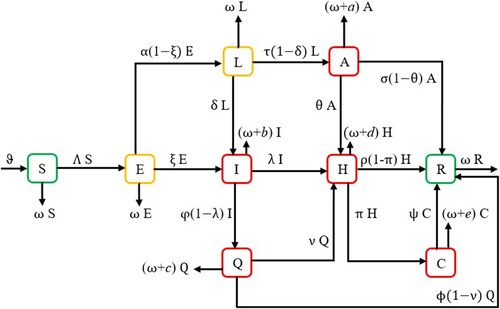
Modeling the dynamics of infectious diseases has attracted a lot of interest in recent years. Such activities are important to disease control and outbreak prevention. It is common to divide the population into distinct classes, or compartments whose sizes change over time, while simulating the transmission dynamics of a contagious disease. The ability of asymptomatic people to spread the disease explains why individual lockdown is important for limiting transmission. In this model, exposed individuals join the lockdown class to lower the risk of the pandemic due to asymptomatic infected people. We divide the total population of Ethiopia into nine different groups, namely, S (susceptible), E (exposed), L (lockdown), A (asymptomatic infected), I (symptomatic infected), Q (quarantile of infected cases), H (hospitalized), C (severe cases) and R (recovered). In this model, the Ethiopian population can be defined in the following form: (16) $P\left(t\right)=S\left(t\right)+E\left(t\right)+L\left(t\right)+A\left(t\right)+I\left(t\right)+Q\left(t\right)+H\left(t\right)+C\left(t\right)+R\left(t\right).$(16) All subgroups have the same natural death rate ω. Some individuals will be removed from the population due to natural death or COVID-19-induced death. Exposed cases become symptomatically infected when they develop coronavirus symptoms and test positive at a rate ξ and the remaining people will be removed at the natural death rate of ω and placed in the lockdown class at a rate of $\alpha (1-\xi )$. Lockdown people get symptomatically infected at a rate of δ, and asymptomatically infected at a rate of $\tau (1-\delta )$. The remaining individuals died naturally. Asymptomatic infected persons recovered from coronavirus disease at a rate of $\sigma (1-\theta )$, acquired symptoms at a rate of θ and exit this class as a result of natural death or due to coronavirus at a rate of $\omega +a$. People who are symptomatically infected transfer into treatment classes at a rate of λ and into home-based isolation and care programs at a rate of $\phi (1-\lambda )$, with the remaining individuals will exit this class with $\omega +b$ natural or COVID-19 caused death rates. This model includes the number of cases transferred from home-based isolation and care to treatment centres for better treatment at a rate of ν. Individuals from quarantine cities recovered from coronavirus disease at a rate of $\varphi (1-\nu )$ and leave this place at a rate of $\omega +c$ due to natural or COVID-19-induced death. Furthermore, some hospitalized infected patients require high-level care and advance to the severe case compartment at a rate of π. The recovery rate from a severe class is denoted by ψ. Individuals are discharged from the hospital, and severe cases with natural and COVID-19-induced death occur at rates of $\omega +d$ and $\omega +e$, respectively. ϑ is the recruitment rate, η is the transmission rate, ℘ is the contact rate from asymptomatically infected people to susceptible people. ϕ is the recovery rate from HBIC (Q), and ρ is the recovery rate from treatment centres. The model is based on the following assumptions:

1. All recruited individuals are assumed to be susceptible at all.

2. Every person has an equal chance of being infected by this pandemic.

3. All model parameters are assumed to have positive values.

4. No reinfection.

These dynamics are described using the ABC fractional-order derivatives as follows: (Figure 1) (17) $\begin{array}{l}{}_0^{ABC}{D}_t^{\gamma }S\left(t\right)={\vartheta }^{\gamma }-(\mathrm{\Lambda }+{\omega }^{\gamma })S\\ {}_0^{ABC}{D}_t^{\gamma }E\left(t\right)=\mathrm{\Lambda }S-({\xi }^{\gamma }+{\alpha }^{\gamma }(1-{\xi }^{\gamma })+{\omega }^{\gamma })E\\ {}_0^{ABC}{D}_t^{\gamma }L\left(t\right)={\alpha }^{\gamma }(1-{\xi }^{\gamma })E-({\delta }^{\gamma }+{\tau }^{\gamma }(1-{\delta }^{\gamma })+{\omega }^{\gamma })L\\ {}_0^{ABC}{D}_t^{\gamma }A\left(t\right)={\tau }^{\gamma }(1-{\delta }^{\gamma })L-({\theta }^{\gamma }+{\sigma }^{\gamma }(1-{\theta }^{\gamma })+{\omega }^{\gamma }+a^{\gamma })A\\ {}_0^{ABC}{D}_t^{\gamma }I\left(t\right)={\xi }^{\gamma }E+{\delta }^{\gamma }L-({\lambda }^{\gamma }+{\phi }^{\gamma }(1-{\lambda }^{\gamma })+{\omega }^{\gamma }+b^{\gamma })I\\ {}_0^{ABC}{D}_t^{\gamma }Q\left(t\right)={\phi }^{\gamma }(1-{\lambda }^{\gamma })I-({\nu }^{\gamma }+{\varphi }^{\gamma }(1-{\nu }^{\gamma })+{\omega }^{\gamma }+c^{\gamma })Q\\ {}_0^{ABC}{D}_t^{\gamma }H\left(t\right)={\theta }^{\gamma }A+{\lambda }^{\gamma }I+{\nu }^{\gamma }Q-({\pi }^{\gamma }+{\rho }^{\gamma }(1-{\pi }^{\gamma })+{\omega }^{\gamma }+d^{\gamma })H\\ {}_0^{ABC}{D}_t^{\gamma }C\left(t\right)={\pi }^{\gamma }H-({\psi }^{\gamma }+{\omega }^{\gamma }+e^{\gamma })C\\ {}_0^{ABC}{D}_t^{\gamma }R\left(t\right)={\sigma }^{\gamma }(1-{\theta }^{\gamma })A+{\varphi }^{\gamma }(1-{\nu }^{\gamma })Q+{\rho }^{\gamma }(1-{\pi }^{\gamma })H+{\psi }^{\gamma }C-{\omega }^{\gamma }R\end{array}\}$(17) where $\mathrm{\Lambda }=\frac{{\eta }^{\gamma }({\mathrm{\wp }}^{\gamma }A+I)}{P}$, with positive starting values: (18) $\begin{array}{rl}{S}_0& =w_1,E_0=w_2,L_0=w_3,A_0=w_4,I_0=w_5,Q_0=w_6,\\ H_0& =w_7,C_0=w_8,R\left(0\right)=w_9.\end{array}$(18)

Figure 1. The COVID-19 model flow diagram.

3.1. Solution positivity and boundedness

Lemma 3.1

The epidemiological feasible region of a model in Equation (17(17) $\begin{array}{l}{}_0^{ABC}{D}_t^{\gamma }S\left(t\right)={\vartheta }^{\gamma }-(\mathrm{\Lambda }+{\omega }^{\gamma })S\\ {}_0^{ABC}{D}_t^{\gamma }E\left(t\right)=\mathrm{\Lambda }S-({\xi }^{\gamma }+{\alpha }^{\gamma }(1-{\xi }^{\gamma })+{\omega }^{\gamma })E\\ {}_0^{ABC}{D}_t^{\gamma }L\left(t\right)={\alpha }^{\gamma }(1-{\xi }^{\gamma })E-({\delta }^{\gamma }+{\tau }^{\gamma }(1-{\delta }^{\gamma })+{\omega }^{\gamma })L\\ {}_0^{ABC}{D}_t^{\gamma }A\left(t\right)={\tau }^{\gamma }(1-{\delta }^{\gamma })L-({\theta }^{\gamma }+{\sigma }^{\gamma }(1-{\theta }^{\gamma })+{\omega }^{\gamma }+a^{\gamma })A\\ {}_0^{ABC}{D}_t^{\gamma }I\left(t\right)={\xi }^{\gamma }E+{\delta }^{\gamma }L-({\lambda }^{\gamma }+{\phi }^{\gamma }(1-{\lambda }^{\gamma })+{\omega }^{\gamma }+b^{\gamma })I\\ {}_0^{ABC}{D}_t^{\gamma }Q\left(t\right)={\phi }^{\gamma }(1-{\lambda }^{\gamma })I-({\nu }^{\gamma }+{\varphi }^{\gamma }(1-{\nu }^{\gamma })+{\omega }^{\gamma }+c^{\gamma })Q\\ {}_0^{ABC}{D}_t^{\gamma }H\left(t\right)={\theta }^{\gamma }A+{\lambda }^{\gamma }I+{\nu }^{\gamma }Q-({\pi }^{\gamma }+{\rho }^{\gamma }(1-{\pi }^{\gamma })+{\omega }^{\gamma }+d^{\gamma })H\\ {}_0^{ABC}{D}_t^{\gamma }C\left(t\right)={\pi }^{\gamma }H-({\psi }^{\gamma }+{\omega }^{\gamma }+e^{\gamma })C\\ {}_0^{ABC}{D}_t^{\gamma }R\left(t\right)={\sigma }^{\gamma }(1-{\theta }^{\gamma })A+{\varphi }^{\gamma }(1-{\nu }^{\gamma })Q+{\rho }^{\gamma }(1-{\pi }^{\gamma })H+{\psi }^{\gamma }C-{\omega }^{\gamma }R\end{array}\}$(17) ) (19) $\mathrm{\Omega }=\left\{S\right(t),E(t),L(t),A(t),I(t),Q(t),H(t),C(t),R(t)\in {\mathbb{R}}_{+}^9:P\left(t\right)\le \frac{{\vartheta }^{\gamma }}{{\omega }^{\gamma }}\},$(19) with positive initial values in Equation (18(18) $\begin{array}{rl}{S}_0& =w_1,E_0=w_2,L_0=w_3,A_0=w_4,I_0=w_5,Q_0=w_6,\\ H_0& =w_7,C_0=w_8,R\left(0\right)=w_9.\end{array}$(18) ) is bounded.

Proof.

The dynamics of the system's entire human population in Equation (17(17) $\begin{array}{l}{}_0^{ABC}{D}_t^{\gamma }S\left(t\right)={\vartheta }^{\gamma }-(\mathrm{\Lambda }+{\omega }^{\gamma })S\\ {}_0^{ABC}{D}_t^{\gamma }E\left(t\right)=\mathrm{\Lambda }S-({\xi }^{\gamma }+{\alpha }^{\gamma }(1-{\xi }^{\gamma })+{\omega }^{\gamma })E\\ {}_0^{ABC}{D}_t^{\gamma }L\left(t\right)={\alpha }^{\gamma }(1-{\xi }^{\gamma })E-({\delta }^{\gamma }+{\tau }^{\gamma }(1-{\delta }^{\gamma })+{\omega }^{\gamma })L\\ {}_0^{ABC}{D}_t^{\gamma }A\left(t\right)={\tau }^{\gamma }(1-{\delta }^{\gamma })L-({\theta }^{\gamma }+{\sigma }^{\gamma }(1-{\theta }^{\gamma })+{\omega }^{\gamma }+a^{\gamma })A\\ {}_0^{ABC}{D}_t^{\gamma }I\left(t\right)={\xi }^{\gamma }E+{\delta }^{\gamma }L-({\lambda }^{\gamma }+{\phi }^{\gamma }(1-{\lambda }^{\gamma })+{\omega }^{\gamma }+b^{\gamma })I\\ {}_0^{ABC}{D}_t^{\gamma }Q\left(t\right)={\phi }^{\gamma }(1-{\lambda }^{\gamma })I-({\nu }^{\gamma }+{\varphi }^{\gamma }(1-{\nu }^{\gamma })+{\omega }^{\gamma }+c^{\gamma })Q\\ {}_0^{ABC}{D}_t^{\gamma }H\left(t\right)={\theta }^{\gamma }A+{\lambda }^{\gamma }I+{\nu }^{\gamma }Q-({\pi }^{\gamma }+{\rho }^{\gamma }(1-{\pi }^{\gamma })+{\omega }^{\gamma }+d^{\gamma })H\\ {}_0^{ABC}{D}_t^{\gamma }C\left(t\right)={\pi }^{\gamma }H-({\psi }^{\gamma }+{\omega }^{\gamma }+e^{\gamma })C\\ {}_0^{ABC}{D}_t^{\gamma }R\left(t\right)={\sigma }^{\gamma }(1-{\theta }^{\gamma })A+{\varphi }^{\gamma }(1-{\nu }^{\gamma })Q+{\rho }^{\gamma }(1-{\pi }^{\gamma })H+{\psi }^{\gamma }C-{\omega }^{\gamma }R\end{array}\}$(17) ) is as follows: (20) ${}_0^{ABC}{D}_t^{\gamma }P\left(t\right)\le {\vartheta }^{\gamma }-{\omega }^{\gamma }P.$(20) Applying the Laplace transform to an inequality (20(20) ${}_0^{ABC}{D}_t^{\gamma }P\left(t\right)\le {\vartheta }^{\gamma }-{\omega }^{\gamma }P.$(20) ), we arrived at: (21) $\begin{array}{rl}P\left(t\right)& \le \left(\frac{M\left(\gamma \right)}{M\left(\gamma \right)+(1-\gamma ){\omega }^{\gamma }}P\right(0)+\frac{(1-\gamma ){\vartheta }^{\gamma }}{M\left(\gamma \right)+(1-\gamma ){\omega }^{\gamma }})E_{\gamma ,1}(-k{t}^{\gamma })\\ & +\frac{\gamma {\vartheta }^{\gamma }}{M\left(\gamma \right)+(1-\gamma ){\omega }^{\gamma }}{E}_{\gamma ,\gamma +1}(-k{t}^{\gamma }),\end{array}$(21) where $k=\frac{\gamma {\omega }^{\gamma }}{M\left(\gamma \right)+(1-\gamma ){\omega }^{\gamma }}$ and $M\left(\gamma \right)=1-\gamma +\frac{\gamma }{\mathrm{\Gamma }\left(\gamma \right)}$.

Using an asymptotic characteristic of the M-L function (Baleanu et al. [46]), we observe that $P\left(t\right)\le \frac{{\vartheta }^{\gamma }}{{\omega }^{\gamma }}$ as $t\to \mathrm{\infty }$. This means that $P\left(t\right)$ (the sum of populations) is bounded, thus, $S\left(t\right)$, $E\left(t\right)$, $L\left(t\right)$, $A\left(t\right)$, $I\left(t\right)$, $Q\left(t\right)$, $H\left(t\right)$, $C\left(t\right)$, and $R\left(t\right)$, are bounded. Hence, Ω is a positive invariant set of the system (17(17) $\begin{array}{l}{}_0^{ABC}{D}_t^{\gamma }S\left(t\right)={\vartheta }^{\gamma }-(\mathrm{\Lambda }+{\omega }^{\gamma })S\\ {}_0^{ABC}{D}_t^{\gamma }E\left(t\right)=\mathrm{\Lambda }S-({\xi }^{\gamma }+{\alpha }^{\gamma }(1-{\xi }^{\gamma })+{\omega }^{\gamma })E\\ {}_0^{ABC}{D}_t^{\gamma }L\left(t\right)={\alpha }^{\gamma }(1-{\xi }^{\gamma })E-({\delta }^{\gamma }+{\tau }^{\gamma }(1-{\delta }^{\gamma })+{\omega }^{\gamma })L\\ {}_0^{ABC}{D}_t^{\gamma }A\left(t\right)={\tau }^{\gamma }(1-{\delta }^{\gamma })L-({\theta }^{\gamma }+{\sigma }^{\gamma }(1-{\theta }^{\gamma })+{\omega }^{\gamma }+a^{\gamma })A\\ {}_0^{ABC}{D}_t^{\gamma }I\left(t\right)={\xi }^{\gamma }E+{\delta }^{\gamma }L-({\lambda }^{\gamma }+{\phi }^{\gamma }(1-{\lambda }^{\gamma })+{\omega }^{\gamma }+b^{\gamma })I\\ {}_0^{ABC}{D}_t^{\gamma }Q\left(t\right)={\phi }^{\gamma }(1-{\lambda }^{\gamma })I-({\nu }^{\gamma }+{\varphi }^{\gamma }(1-{\nu }^{\gamma })+{\omega }^{\gamma }+c^{\gamma })Q\\ {}_0^{ABC}{D}_t^{\gamma }H\left(t\right)={\theta }^{\gamma }A+{\lambda }^{\gamma }I+{\nu }^{\gamma }Q-({\pi }^{\gamma }+{\rho }^{\gamma }(1-{\pi }^{\gamma })+{\omega }^{\gamma }+d^{\gamma })H\\ {}_0^{ABC}{D}_t^{\gamma }C\left(t\right)={\pi }^{\gamma }H-({\psi }^{\gamma }+{\omega }^{\gamma }+e^{\gamma })C\\ {}_0^{ABC}{D}_t^{\gamma }R\left(t\right)={\sigma }^{\gamma }(1-{\theta }^{\gamma })A+{\varphi }^{\gamma }(1-{\nu }^{\gamma })Q+{\rho }^{\gamma }(1-{\pi }^{\gamma })H+{\psi }^{\gamma }C-{\omega }^{\gamma }R\end{array}\}$(17) ).

Theorem 3.1

For all $t\ge 0$, the solutions of a system in Equation (17(17) $\begin{array}{l}{}_0^{ABC}{D}_t^{\gamma }S\left(t\right)={\vartheta }^{\gamma }-(\mathrm{\Lambda }+{\omega }^{\gamma })S\\ {}_0^{ABC}{D}_t^{\gamma }E\left(t\right)=\mathrm{\Lambda }S-({\xi }^{\gamma }+{\alpha }^{\gamma }(1-{\xi }^{\gamma })+{\omega }^{\gamma })E\\ {}_0^{ABC}{D}_t^{\gamma }L\left(t\right)={\alpha }^{\gamma }(1-{\xi }^{\gamma })E-({\delta }^{\gamma }+{\tau }^{\gamma }(1-{\delta }^{\gamma })+{\omega }^{\gamma })L\\ {}_0^{ABC}{D}_t^{\gamma }A\left(t\right)={\tau }^{\gamma }(1-{\delta }^{\gamma })L-({\theta }^{\gamma }+{\sigma }^{\gamma }(1-{\theta }^{\gamma })+{\omega }^{\gamma }+a^{\gamma })A\\ {}_0^{ABC}{D}_t^{\gamma }I\left(t\right)={\xi }^{\gamma }E+{\delta }^{\gamma }L-({\lambda }^{\gamma }+{\phi }^{\gamma }(1-{\lambda }^{\gamma })+{\omega }^{\gamma }+b^{\gamma })I\\ {}_0^{ABC}{D}_t^{\gamma }Q\left(t\right)={\phi }^{\gamma }(1-{\lambda }^{\gamma })I-({\nu }^{\gamma }+{\varphi }^{\gamma }(1-{\nu }^{\gamma })+{\omega }^{\gamma }+c^{\gamma })Q\\ {}_0^{ABC}{D}_t^{\gamma }H\left(t\right)={\theta }^{\gamma }A+{\lambda }^{\gamma }I+{\nu }^{\gamma }Q-({\pi }^{\gamma }+{\rho }^{\gamma }(1-{\pi }^{\gamma })+{\omega }^{\gamma }+d^{\gamma })H\\ {}_0^{ABC}{D}_t^{\gamma }C\left(t\right)={\pi }^{\gamma }H-({\psi }^{\gamma }+{\omega }^{\gamma }+e^{\gamma })C\\ {}_0^{ABC}{D}_t^{\gamma }R\left(t\right)={\sigma }^{\gamma }(1-{\theta }^{\gamma })A+{\varphi }^{\gamma }(1-{\nu }^{\gamma })Q+{\rho }^{\gamma }(1-{\pi }^{\gamma })H+{\psi }^{\gamma }C-{\omega }^{\gamma }R\end{array}\}$(17) ) with positive beginning conditions in (18(18) $\begin{array}{rl}{S}_0& =w_1,E_0=w_2,L_0=w_3,A_0=w_4,I_0=w_5,Q_0=w_6,\\ H_0& =w_7,C_0=w_8,R\left(0\right)=w_9.\end{array}$(18) ) are positive.

Proof.

From the first equation of a system in Equation (17(17) $\begin{array}{l}{}_0^{ABC}{D}_t^{\gamma }S\left(t\right)={\vartheta }^{\gamma }-(\mathrm{\Lambda }+{\omega }^{\gamma })S\\ {}_0^{ABC}{D}_t^{\gamma }E\left(t\right)=\mathrm{\Lambda }S-({\xi }^{\gamma }+{\alpha }^{\gamma }(1-{\xi }^{\gamma })+{\omega }^{\gamma })E\\ {}_0^{ABC}{D}_t^{\gamma }L\left(t\right)={\alpha }^{\gamma }(1-{\xi }^{\gamma })E-({\delta }^{\gamma }+{\tau }^{\gamma }(1-{\delta }^{\gamma })+{\omega }^{\gamma })L\\ {}_0^{ABC}{D}_t^{\gamma }A\left(t\right)={\tau }^{\gamma }(1-{\delta }^{\gamma })L-({\theta }^{\gamma }+{\sigma }^{\gamma }(1-{\theta }^{\gamma })+{\omega }^{\gamma }+a^{\gamma })A\\ {}_0^{ABC}{D}_t^{\gamma }I\left(t\right)={\xi }^{\gamma }E+{\delta }^{\gamma }L-({\lambda }^{\gamma }+{\phi }^{\gamma }(1-{\lambda }^{\gamma })+{\omega }^{\gamma }+b^{\gamma })I\\ {}_0^{ABC}{D}_t^{\gamma }Q\left(t\right)={\phi }^{\gamma }(1-{\lambda }^{\gamma })I-({\nu }^{\gamma }+{\varphi }^{\gamma }(1-{\nu }^{\gamma })+{\omega }^{\gamma }+c^{\gamma })Q\\ {}_0^{ABC}{D}_t^{\gamma }H\left(t\right)={\theta }^{\gamma }A+{\lambda }^{\gamma }I+{\nu }^{\gamma }Q-({\pi }^{\gamma }+{\rho }^{\gamma }(1-{\pi }^{\gamma })+{\omega }^{\gamma }+d^{\gamma })H\\ {}_0^{ABC}{D}_t^{\gamma }C\left(t\right)={\pi }^{\gamma }H-({\psi }^{\gamma }+{\omega }^{\gamma }+e^{\gamma })C\\ {}_0^{ABC}{D}_t^{\gamma }R\left(t\right)={\sigma }^{\gamma }(1-{\theta }^{\gamma })A+{\varphi }^{\gamma }(1-{\nu }^{\gamma })Q+{\rho }^{\gamma }(1-{\pi }^{\gamma })H+{\psi }^{\gamma }C-{\omega }^{\gamma }R\end{array}\}$(17) ), we have: (22) ${}_0^{ABC}{D}_t^{\gamma }S\left(t\right)={\vartheta }^{\gamma }-(\mathrm{\Lambda }+{\omega }^{\gamma })S\ge -(\mathrm{\Lambda }+{\omega }^{\gamma })S,$(22) where $\mathrm{\Lambda }=\frac{{\eta }^{\gamma }({\mathrm{\wp }}^{\gamma }A+I)}{P}$. We have ${\mathrm{\wp }}^{\gamma }A+I$ bounded by a constant ${\mathrm{\Lambda }}_0$ according to Lemma (3.1). (23) ${}_0^{ABC}{D}_t^{\gamma }S\left(t\right)\ge -wS\left(t\right),$(23) where w is a constant equal to $\frac{{\mathrm{\Lambda }}_0}{P}+{\omega }^{\gamma }$.

Applying a Laplace transform to an inequality (23(23) ${}_0^{ABC}{D}_t^{\gamma }S\left(t\right)\ge -wS\left(t\right),$(23) ), we arrived at: (24) $S\left(t\right)\ge \frac{M\left(\gamma \right)}{M\left(\gamma \right)+(1-\gamma )w}S\left(0\right)E_{\gamma ,1}(-\frac{\gamma w}{M\left(\gamma \right)+(1-\gamma )w}{t}^{\gamma }).$(24) Since $E_{\gamma ,1}(-\frac{\gamma w}{M\left(\gamma \right)+(1-\gamma )w}{t}^{\gamma })>0$ and $S\left(0\right)\ge 0$, then $S\left(t\right)$ is positive. It is easy to show that the system's other state variables remain positive for all $t\ge 0$ by following the above steps.

3.2. Stability analysis

For a system in Equation (17(17) $\begin{array}{l}{}_0^{ABC}{D}_t^{\gamma }S\left(t\right)={\vartheta }^{\gamma }-(\mathrm{\Lambda }+{\omega }^{\gamma })S\\ {}_0^{ABC}{D}_t^{\gamma }E\left(t\right)=\mathrm{\Lambda }S-({\xi }^{\gamma }+{\alpha }^{\gamma }(1-{\xi }^{\gamma })+{\omega }^{\gamma })E\\ {}_0^{ABC}{D}_t^{\gamma }L\left(t\right)={\alpha }^{\gamma }(1-{\xi }^{\gamma })E-({\delta }^{\gamma }+{\tau }^{\gamma }(1-{\delta }^{\gamma })+{\omega }^{\gamma })L\\ {}_0^{ABC}{D}_t^{\gamma }A\left(t\right)={\tau }^{\gamma }(1-{\delta }^{\gamma })L-({\theta }^{\gamma }+{\sigma }^{\gamma }(1-{\theta }^{\gamma })+{\omega }^{\gamma }+a^{\gamma })A\\ {}_0^{ABC}{D}_t^{\gamma }I\left(t\right)={\xi }^{\gamma }E+{\delta }^{\gamma }L-({\lambda }^{\gamma }+{\phi }^{\gamma }(1-{\lambda }^{\gamma })+{\omega }^{\gamma }+b^{\gamma })I\\ {}_0^{ABC}{D}_t^{\gamma }Q\left(t\right)={\phi }^{\gamma }(1-{\lambda }^{\gamma })I-({\nu }^{\gamma }+{\varphi }^{\gamma }(1-{\nu }^{\gamma })+{\omega }^{\gamma }+c^{\gamma })Q\\ {}_0^{ABC}{D}_t^{\gamma }H\left(t\right)={\theta }^{\gamma }A+{\lambda }^{\gamma }I+{\nu }^{\gamma }Q-({\pi }^{\gamma }+{\rho }^{\gamma }(1-{\pi }^{\gamma })+{\omega }^{\gamma }+d^{\gamma })H\\ {}_0^{ABC}{D}_t^{\gamma }C\left(t\right)={\pi }^{\gamma }H-({\psi }^{\gamma }+{\omega }^{\gamma }+e^{\gamma })C\\ {}_0^{ABC}{D}_t^{\gamma }R\left(t\right)={\sigma }^{\gamma }(1-{\theta }^{\gamma })A+{\varphi }^{\gamma }(1-{\nu }^{\gamma })Q+{\rho }^{\gamma }(1-{\pi }^{\gamma })H+{\psi }^{\gamma }C-{\omega }^{\gamma }R\end{array}\}$(17) ), the COVID-19-free equilibrium point is: (25) ${\mathfrak{F}}_0=(\frac{{\vartheta }^{\gamma }}{{\omega }^{\gamma }},0,0,0,0,0,0,0,0).$(25) At $\mathfrak{F}0$, the transmission and transition matrices are: $\mathrm{X}=\left[\begin{array}{ccccccc}0& 0& {\eta }^{\gamma }{\mathrm{\wp }}^{\gamma }& {\eta }^{\gamma }& 0& 0& 0\\ 0& 0& 0& 0& 0& 0& 0\\ 0& 0& 0& 0& 0& 0& 0\\ 0& 0& 0& 0& 0& 0& 0\\ 0& 0& 0& 0& 0& 0& 0\\ 0& 0& 0& 0& 0& 0& 0\\ 0& 0& 0& 0& 0& 0& 0\end{array}\right],$ and $\mathrm{Y}=\left[\begin{array}{ccccccc}{u}_1& 0& 0& 0& 0& 0& 0\\ -{\alpha }^{\gamma }(1-{\xi }^{\gamma })& u_2& 0& 0& 0& 0& 0\\ 0& -{\tau }^{\gamma }(1-{\delta }^{\gamma })& u_3& 0& 0& 0& 0\\ -{\xi }^{\gamma }& -{\delta }^{\gamma }& 0& u_4& 0& 0& 0\\ 0& 0& 0& -{\phi }^{\gamma }(1-{\lambda }^{\gamma })& u_5& 0& 0\\ 0& 0& -{\theta }^{\gamma }& -{\lambda }^{\gamma }& -{\nu }^{\gamma }& u_6& 0\\ 0& 0& 0& 0& 0& -{\pi }^{\gamma }& u_7\end{array}\right].$ where $\begin{array}{rl}{u}_1& ={\xi }^{\gamma }+{\alpha }^{\gamma }(1-{\xi }^{\gamma })+{\omega }^{\gamma },u_2={\delta }^{\gamma }+{\tau }^{\gamma }(1-{\delta }^{\gamma })+{\omega }^{\gamma },\\ u_3& ={\theta }^{\gamma }+{\sigma }^{\gamma }(1-{\theta }^{\gamma })+{\omega }^{\gamma }+a^{\gamma },\\ u_4& ={\lambda }^{\gamma }+{\phi }^{\gamma }(1-{\lambda }^{\gamma })+{\omega }^{\gamma }+b^{\gamma },u_5={\nu }^{\gamma }+{\varphi }^{\gamma }(1-{\nu }^{\gamma })+{\omega }^{\gamma }+c^{\gamma },\\ u_6& ={\pi }^{\gamma }+{\rho }^{\gamma }(1-{\pi }^{\gamma })+{\omega }^{\gamma }+d^{\gamma },\\ u_7& ={\psi }^{\gamma }+{\omega }^{\gamma }+e^{\gamma }.\end{array}$ The dominant eigenvalue of the next generation matrix $\mathrm{X}{\mathrm{Y}}^{-1}$ is the required fundamental reproduction number, given by: (26) ${\mathfrak{R}}_0=\frac{{\eta }^{\gamma }{\alpha }^{\gamma }(1-{\xi }^{\gamma })}{u_1{u}_2}(\frac{{\mathrm{\wp }}^{\gamma }{\tau }^{\gamma }(1-{\delta }^{\gamma })}{u_3}+\frac{{\delta }^{\gamma }}{u_4})+\frac{{\eta }^{\gamma }{\xi }^{\gamma }}{u_1{u}_4}.$(26)

Theorem 3.2

The disease-free equilibrium point ${\mathfrak{F}}_0$ in Equation (25(25) ${\mathfrak{F}}_0=(\frac{{\vartheta }^{\gamma }}{{\omega }^{\gamma }},0,0,0,0,0,0,0,0).$(25) ) is locally asymptotically stable if ${\mathfrak{R}}_0<1$ and unstable if ${\mathfrak{R}}_0>1$.

Proof.

The local stability of the system in Equation (17(17) $\begin{array}{l}{}_0^{ABC}{D}_t^{\gamma }S\left(t\right)={\vartheta }^{\gamma }-(\mathrm{\Lambda }+{\omega }^{\gamma })S\\ {}_0^{ABC}{D}_t^{\gamma }E\left(t\right)=\mathrm{\Lambda }S-({\xi }^{\gamma }+{\alpha }^{\gamma }(1-{\xi }^{\gamma })+{\omega }^{\gamma })E\\ {}_0^{ABC}{D}_t^{\gamma }L\left(t\right)={\alpha }^{\gamma }(1-{\xi }^{\gamma })E-({\delta }^{\gamma }+{\tau }^{\gamma }(1-{\delta }^{\gamma })+{\omega }^{\gamma })L\\ {}_0^{ABC}{D}_t^{\gamma }A\left(t\right)={\tau }^{\gamma }(1-{\delta }^{\gamma })L-({\theta }^{\gamma }+{\sigma }^{\gamma }(1-{\theta }^{\gamma })+{\omega }^{\gamma }+a^{\gamma })A\\ {}_0^{ABC}{D}_t^{\gamma }I\left(t\right)={\xi }^{\gamma }E+{\delta }^{\gamma }L-({\lambda }^{\gamma }+{\phi }^{\gamma }(1-{\lambda }^{\gamma })+{\omega }^{\gamma }+b^{\gamma })I\\ {}_0^{ABC}{D}_t^{\gamma }Q\left(t\right)={\phi }^{\gamma }(1-{\lambda }^{\gamma })I-({\nu }^{\gamma }+{\varphi }^{\gamma }(1-{\nu }^{\gamma })+{\omega }^{\gamma }+c^{\gamma })Q\\ {}_0^{ABC}{D}_t^{\gamma }H\left(t\right)={\theta }^{\gamma }A+{\lambda }^{\gamma }I+{\nu }^{\gamma }Q-({\pi }^{\gamma }+{\rho }^{\gamma }(1-{\pi }^{\gamma })+{\omega }^{\gamma }+d^{\gamma })H\\ {}_0^{ABC}{D}_t^{\gamma }C\left(t\right)={\pi }^{\gamma }H-({\psi }^{\gamma }+{\omega }^{\gamma }+e^{\gamma })C\\ {}_0^{ABC}{D}_t^{\gamma }R\left(t\right)={\sigma }^{\gamma }(1-{\theta }^{\gamma })A+{\varphi }^{\gamma }(1-{\nu }^{\gamma })Q+{\rho }^{\gamma }(1-{\pi }^{\gamma })H+{\psi }^{\gamma }C-{\omega }^{\gamma }R\end{array}\}$(17) ) is investigated using the Jacobian matrix of the model (17(17) $\begin{array}{l}{}_0^{ABC}{D}_t^{\gamma }S\left(t\right)={\vartheta }^{\gamma }-(\mathrm{\Lambda }+{\omega }^{\gamma })S\\ {}_0^{ABC}{D}_t^{\gamma }E\left(t\right)=\mathrm{\Lambda }S-({\xi }^{\gamma }+{\alpha }^{\gamma }(1-{\xi }^{\gamma })+{\omega }^{\gamma })E\\ {}_0^{ABC}{D}_t^{\gamma }L\left(t\right)={\alpha }^{\gamma }(1-{\xi }^{\gamma })E-({\delta }^{\gamma }+{\tau }^{\gamma }(1-{\delta }^{\gamma })+{\omega }^{\gamma })L\\ {}_0^{ABC}{D}_t^{\gamma }A\left(t\right)={\tau }^{\gamma }(1-{\delta }^{\gamma })L-({\theta }^{\gamma }+{\sigma }^{\gamma }(1-{\theta }^{\gamma })+{\omega }^{\gamma }+a^{\gamma })A\\ {}_0^{ABC}{D}_t^{\gamma }I\left(t\right)={\xi }^{\gamma }E+{\delta }^{\gamma }L-({\lambda }^{\gamma }+{\phi }^{\gamma }(1-{\lambda }^{\gamma })+{\omega }^{\gamma }+b^{\gamma })I\\ {}_0^{ABC}{D}_t^{\gamma }Q\left(t\right)={\phi }^{\gamma }(1-{\lambda }^{\gamma })I-({\nu }^{\gamma }+{\varphi }^{\gamma }(1-{\nu }^{\gamma })+{\omega }^{\gamma }+c^{\gamma })Q\\ {}_0^{ABC}{D}_t^{\gamma }H\left(t\right)={\theta }^{\gamma }A+{\lambda }^{\gamma }I+{\nu }^{\gamma }Q-({\pi }^{\gamma }+{\rho }^{\gamma }(1-{\pi }^{\gamma })+{\omega }^{\gamma }+d^{\gamma })H\\ {}_0^{ABC}{D}_t^{\gamma }C\left(t\right)={\pi }^{\gamma }H-({\psi }^{\gamma }+{\omega }^{\gamma }+e^{\gamma })C\\ {}_0^{ABC}{D}_t^{\gamma }R\left(t\right)={\sigma }^{\gamma }(1-{\theta }^{\gamma })A+{\varphi }^{\gamma }(1-{\nu }^{\gamma })Q+{\rho }^{\gamma }(1-{\pi }^{\gamma })H+{\psi }^{\gamma }C-{\omega }^{\gamma }R\end{array}\}$(17) ) computed at ${\mathfrak{F}}_0$, given by: (27) $\begin{array}{rl}{J}_{{\mathfrak{F}}_0}& =[\begin{array}{ccccc}-{\omega }^{\gamma }& 0& 0& -{\eta }^{\gamma }{\mathrm{\wp }}^{\gamma }& -{\eta }^{\gamma }\\ 0& -u_1& 0& {\eta }^{\gamma }{\mathrm{\wp }}^{\gamma }& {\eta }^{\gamma }\\ 0& {\alpha }^{\gamma }(1-{\xi }^{\gamma })& -u_2& 0& 0\\ 0& 0& {\tau }^{\gamma }(1-{\delta }^{\gamma })& -u_3& 0\\ 0& {\xi }^{\gamma }& {\delta }^{\gamma }& 0& -u_4\\ 0& 0& 0& 0& {\phi }^{\gamma }(1-{\lambda }^{\gamma })\\ 0& 0& 0& {\theta }^{\gamma }& {\lambda }^{\gamma }\\ 0& 0& 0& 0& 0\\ 0& 0& 0& {\sigma }^{\gamma }(1-{\theta }^{\gamma })& 0\end{array}\\ & \begin{array}{cccc}0& 0& 0& 0\\ 0& 0& 0& 0\\ 0& 0& 0& 0\\ 0& 0& 0& 0\\ 0& 0& 0& 0\\ -u_5& 0& 0& 0\\ {\nu }^{\gamma }& -u_6& 0& 0\\ 0& {\pi }^{\gamma }& -u_7& 0\\ {\varphi }^{\gamma }(1-{\nu }^{\gamma })& {\rho }^{\gamma }(1-{\pi }^{\gamma })& {\psi }^{\gamma }& -{\omega }^{\gamma }\end{array}],\end{array}$(27) Following Equation (27(27) $\begin{array}{rl}{J}_{{\mathfrak{F}}_0}& =[\begin{array}{ccccc}-{\omega }^{\gamma }& 0& 0& -{\eta }^{\gamma }{\mathrm{\wp }}^{\gamma }& -{\eta }^{\gamma }\\ 0& -u_1& 0& {\eta }^{\gamma }{\mathrm{\wp }}^{\gamma }& {\eta }^{\gamma }\\ 0& {\alpha }^{\gamma }(1-{\xi }^{\gamma })& -u_2& 0& 0\\ 0& 0& {\tau }^{\gamma }(1-{\delta }^{\gamma })& -u_3& 0\\ 0& {\xi }^{\gamma }& {\delta }^{\gamma }& 0& -u_4\\ 0& 0& 0& 0& {\phi }^{\gamma }(1-{\lambda }^{\gamma })\\ 0& 0& 0& {\theta }^{\gamma }& {\lambda }^{\gamma }\\ 0& 0& 0& 0& 0\\ 0& 0& 0& {\sigma }^{\gamma }(1-{\theta }^{\gamma })& 0\end{array}\\ & \begin{array}{cccc}0& 0& 0& 0\\ 0& 0& 0& 0\\ 0& 0& 0& 0\\ 0& 0& 0& 0\\ 0& 0& 0& 0\\ -u_5& 0& 0& 0\\ {\nu }^{\gamma }& -u_6& 0& 0\\ 0& {\pi }^{\gamma }& -u_7& 0\\ {\varphi }^{\gamma }(1-{\nu }^{\gamma })& {\rho }^{\gamma }(1-{\pi }^{\gamma })& {\psi }^{\gamma }& -{\omega }^{\gamma }\end{array}],\end{array}$(27) ), five of the eigenvalues are negative. That are ${\psi }_1={\psi }_2=-{\omega }^{\gamma },{\psi }_3=-({\nu }^{\gamma }+{\varphi }^{\gamma }(1-{\nu }^{\gamma })+{\omega }^{\gamma }+c^{\gamma }),{\psi }_4=-({\pi }^{\gamma }+{\rho }^{\gamma }(1-{\pi }^{\gamma })+{\omega }^{\gamma }+d^{\gamma }),{\psi }_5=-({\psi }^{\gamma }+{\omega }^{\gamma }+e^{\gamma })$. The following characteristic equation can be used to find the remaining eigenvalues: ${\psi }^4+b_1{\psi }^3+b_2{\psi }^2+b_3\psi +b_4=0,$ where $\begin{array}{rl}{b}_1& =u_1+u_2+u_3+u_4,b_2=\frac{u_4{\eta }^{\gamma }{\alpha }^{\gamma }(1-{\xi }^{\gamma })}{u_2}(\frac{{\mathrm{\wp }}^{\gamma }{\tau }^{\gamma }(1-{\delta }^{\gamma })}{u_3}+\frac{{\delta }^{\gamma }}{u_4})\\ & +u_1{u}_4(1-{\mathfrak{R}}_0)+(u_1+u_4)(u_2+u_3)+u_2{u}_3.\\ b_3& ={\eta }^{\gamma }{\alpha }^{\gamma }(1-{\xi }^{\gamma })(\frac{u_3{\delta }^{\gamma }}{u_4}+\frac{u_4{\mathrm{\wp }}^{\gamma }{\tau }^{\gamma }(1-{\delta }^{\gamma })}{u_3}+\frac{{\mathrm{\wp }}^{\gamma }{\tau }^{\gamma }(1-{\delta }^{\gamma })u_4}{u_1{u}_2}+\frac{{\delta }^{\gamma }{u}_3}{u_1{u}_2})\\ & +\frac{u_2{u}_3{\eta }^{\gamma }{\xi }^{\gamma }}{u_4+u_1(u_2{u}_3+u_2{u}_4+u_3{u}_4)(1-{\mathfrak{R}}_0)+u_2{u}_3{u}_4},b_4=u_1{u}_2{u}_3{u}_4(1-{\mathfrak{R}}_0).\end{array}$ When ${\mathfrak{R}}_0<1$, the coefficients $b_2$, $b_3$ and $b_4$ are all positive, and the coefficient $b_1$ is clearly positive. So, ${\mathfrak{F}}_0$ is locally asymptotically stable if ${\mathfrak{R}}_0<1$ and unstable if ${\mathfrak{R}}_0>1.$

By setting the system equations in Equation (17(17) $\begin{array}{l}{}_0^{ABC}{D}_t^{\gamma }S\left(t\right)={\vartheta }^{\gamma }-(\mathrm{\Lambda }+{\omega }^{\gamma })S\\ {}_0^{ABC}{D}_t^{\gamma }E\left(t\right)=\mathrm{\Lambda }S-({\xi }^{\gamma }+{\alpha }^{\gamma }(1-{\xi }^{\gamma })+{\omega }^{\gamma })E\\ {}_0^{ABC}{D}_t^{\gamma }L\left(t\right)={\alpha }^{\gamma }(1-{\xi }^{\gamma })E-({\delta }^{\gamma }+{\tau }^{\gamma }(1-{\delta }^{\gamma })+{\omega }^{\gamma })L\\ {}_0^{ABC}{D}_t^{\gamma }A\left(t\right)={\tau }^{\gamma }(1-{\delta }^{\gamma })L-({\theta }^{\gamma }+{\sigma }^{\gamma }(1-{\theta }^{\gamma })+{\omega }^{\gamma }+a^{\gamma })A\\ {}_0^{ABC}{D}_t^{\gamma }I\left(t\right)={\xi }^{\gamma }E+{\delta }^{\gamma }L-({\lambda }^{\gamma }+{\phi }^{\gamma }(1-{\lambda }^{\gamma })+{\omega }^{\gamma }+b^{\gamma })I\\ {}_0^{ABC}{D}_t^{\gamma }Q\left(t\right)={\phi }^{\gamma }(1-{\lambda }^{\gamma })I-({\nu }^{\gamma }+{\varphi }^{\gamma }(1-{\nu }^{\gamma })+{\omega }^{\gamma }+c^{\gamma })Q\\ {}_0^{ABC}{D}_t^{\gamma }H\left(t\right)={\theta }^{\gamma }A+{\lambda }^{\gamma }I+{\nu }^{\gamma }Q-({\pi }^{\gamma }+{\rho }^{\gamma }(1-{\pi }^{\gamma })+{\omega }^{\gamma }+d^{\gamma })H\\ {}_0^{ABC}{D}_t^{\gamma }C\left(t\right)={\pi }^{\gamma }H-({\psi }^{\gamma }+{\omega }^{\gamma }+e^{\gamma })C\\ {}_0^{ABC}{D}_t^{\gamma }R\left(t\right)={\sigma }^{\gamma }(1-{\theta }^{\gamma })A+{\varphi }^{\gamma }(1-{\nu }^{\gamma })Q+{\rho }^{\gamma }(1-{\pi }^{\gamma })H+{\psi }^{\gamma }C-{\omega }^{\gamma }R\end{array}\}$(17) ) to zero and solving them simultaneously, we can find the infectious equilibrium point ${\mathfrak{F}}^{\ast }=({\mathcal{S}}^{\ast },{\mathcal{E}}^{\ast },{\mathcal{L}}^{\ast },{\mathcal{A}}^{\ast },{\mathcal{I}}^{\ast },{\mathcal{Q}}^{\ast },{\mathcal{H}}^{\ast },{\mathcal{C}}^{\ast },{\mathcal{R}}^{\ast },)$

where $\begin{array}{rl}{\mathcal{S}}^{\ast }& =\frac{{\vartheta }^{\gamma }}{{\omega }^{\gamma }}-\frac{u_1}{{\omega }^{\gamma }}{\mathcal{E}}^{\ast },{\mathcal{L}}^{\ast }=\frac{{\alpha }^{\gamma }(1-{\xi }^{\gamma })}{u_2}{\mathcal{E}}^{\ast },\\ {\mathcal{A}}^{\ast }& =\frac{{\tau }^{\gamma }{\alpha }^{\gamma }(1-{\xi }^{\gamma })(1-{\delta }^{\gamma })}{u_2{u}_3}{\mathcal{E}}^{\ast },{\mathcal{I}}^{\ast }=(\frac{{\xi }^{\gamma }}{u_4}+\frac{{\delta }^{\gamma }{\alpha }^{\gamma }(1-{\xi }^{\gamma })}{u_2{u}_4}){\mathcal{E}}^{\ast },\\ Q^{\ast }& =\frac{{\phi }^{\gamma }(1-{\lambda }^{\gamma })}{u_4{u}_5}({\xi }^{\gamma }+\frac{{\delta }^{\gamma }{\alpha }^{\gamma }(1-{\xi }^{\gamma })}{u_2}){\mathcal{E}}^{\ast },\\ {\mathcal{H}}^{\ast }& =\frac{\frac{{\theta }^{\gamma }{\tau }^{\gamma }{\alpha }^{\gamma }(1-{\xi }^{\gamma })(1-{\delta }^{\gamma })}{u_2{u}_3}+({\lambda }^{\gamma }+\frac{{\nu }^{\gamma }{\phi }^{\gamma }(1-{\lambda }^{\gamma })}{u_5})(\frac{{\xi }^{\gamma }}{u_4}+\frac{{\delta }^{\gamma }{\alpha }^{\gamma }(1-{\xi }^{\gamma })}{u_2{u}_4})}{u_6}{\mathcal{E}}^{\ast },\\ {\mathcal{C}}^{\ast }& =\frac{\frac{{\theta }^{\gamma }{\tau }^{\gamma }{\alpha }^{\gamma }(1-{\xi }^{\gamma })(1-{\delta }^{\gamma })}{u_2{u}_3}+({\lambda }^{\gamma }+\frac{{\nu }^{\gamma }{\phi }^{\gamma }(1-{\lambda }^{\gamma })}{u_5})(\frac{{\xi }^{\gamma }}{u_4}+\frac{{\delta }^{\gamma }{\alpha }^{\gamma }(1-{\xi }^{\gamma })}{u_2{u}_4})}{u_6{u}_7}{\pi }^{\gamma }{\mathcal{E}}^{\ast },\\ {\mathcal{R}}^{\ast }& =\frac{{\sigma }^{\gamma }(1-{\theta }^{\gamma }){\mathcal{A}}^{\ast }+{\varphi }^{\gamma }(1-{\nu }^{\gamma }){\mathcal{Q}}^{\ast }+{\rho }^{\gamma }(1-{\pi }^{\gamma }){\mathcal{H}}^{\ast }+{\psi }^{\gamma }{\mathcal{C}}^{\ast }}{{\omega }^{\gamma }}.\end{array}$ and substituting ${\mathcal{S}}^{\ast },{\mathcal{A}}^{\ast },\mathrm{a}\mathrm{n}\mathrm{d}{\mathcal{I}}^{\ast }$ on the second equation of (17(17) $\begin{array}{l}{}_0^{ABC}{D}_t^{\gamma }S\left(t\right)={\vartheta }^{\gamma }-(\mathrm{\Lambda }+{\omega }^{\gamma })S\\ {}_0^{ABC}{D}_t^{\gamma }E\left(t\right)=\mathrm{\Lambda }S-({\xi }^{\gamma }+{\alpha }^{\gamma }(1-{\xi }^{\gamma })+{\omega }^{\gamma })E\\ {}_0^{ABC}{D}_t^{\gamma }L\left(t\right)={\alpha }^{\gamma }(1-{\xi }^{\gamma })E-({\delta }^{\gamma }+{\tau }^{\gamma }(1-{\delta }^{\gamma })+{\omega }^{\gamma })L\\ {}_0^{ABC}{D}_t^{\gamma }A\left(t\right)={\tau }^{\gamma }(1-{\delta }^{\gamma })L-({\theta }^{\gamma }+{\sigma }^{\gamma }(1-{\theta }^{\gamma })+{\omega }^{\gamma }+a^{\gamma })A\\ {}_0^{ABC}{D}_t^{\gamma }I\left(t\right)={\xi }^{\gamma }E+{\delta }^{\gamma }L-({\lambda }^{\gamma }+{\phi }^{\gamma }(1-{\lambda }^{\gamma })+{\omega }^{\gamma }+b^{\gamma })I\\ {}_0^{ABC}{D}_t^{\gamma }Q\left(t\right)={\phi }^{\gamma }(1-{\lambda }^{\gamma })I-({\nu }^{\gamma }+{\varphi }^{\gamma }(1-{\nu }^{\gamma })+{\omega }^{\gamma }+c^{\gamma })Q\\ {}_0^{ABC}{D}_t^{\gamma }H\left(t\right)={\theta }^{\gamma }A+{\lambda }^{\gamma }I+{\nu }^{\gamma }Q-({\pi }^{\gamma }+{\rho }^{\gamma }(1-{\pi }^{\gamma })+{\omega }^{\gamma }+d^{\gamma })H\\ {}_0^{ABC}{D}_t^{\gamma }C\left(t\right)={\pi }^{\gamma }H-({\psi }^{\gamma }+{\omega }^{\gamma }+e^{\gamma })C\\ {}_0^{ABC}{D}_t^{\gamma }R\left(t\right)={\sigma }^{\gamma }(1-{\theta }^{\gamma })A+{\varphi }^{\gamma }(1-{\nu }^{\gamma })Q+{\rho }^{\gamma }(1-{\pi }^{\gamma })H+{\psi }^{\gamma }C-{\omega }^{\gamma }R\end{array}\}$(17) ), we arrived at: $\frac{\frac{{\eta }^{\gamma }{\mathrm{\wp }}^{\gamma }{\tau }^{\gamma }{\alpha }^{\gamma }(1-{\xi }^{\gamma })(1-{\delta }^{\gamma })}{u_2{u}_3}{\mathcal{E}}^{\ast }+(\frac{{\eta }^{\gamma }{\xi }^{\gamma }}{u_4}+\frac{{\eta }^{\gamma }{\delta }^{\gamma }{\alpha }^{\gamma }(1-{\xi }^{\gamma })}{u_2{u}_4}){\mathcal{E}}^{\ast }}{P}(\frac{{\vartheta }^{\gamma }}{{\omega }^{\gamma }}-\frac{u_1}{{\omega }^{\gamma }}{\mathcal{E}}^{\ast })-u_1{\mathcal{E}}^{\ast }=0.$ Taking ${\vartheta }^{\gamma }={\omega }^{\gamma }P$, then we have: $\begin{array}{rl}& (\frac{{\eta }^{\gamma }{\mathrm{\wp }}^{\gamma }{\tau }^{\gamma }{\alpha }^{\gamma }(1-{\xi }^{\gamma })(1-{\delta }^{\gamma })}{u_1{u}_2{u}_3}+\frac{{\eta }^{\gamma }{\delta }^{\gamma }{\alpha }^{\gamma }(1-{\xi }^{\gamma })}{u_1{u}_2{u}_4}+\frac{{\eta }^{\gamma }{\xi }^{\gamma }}{u_1{u}_4})(1-\frac{u_1}{{\vartheta }^{\gamma }}{\mathcal{E}}^{\ast })-1=0,\\ & {\mathcal{E}}^{\ast }=\frac{{\vartheta }^{\gamma }}{u_1}(1-\frac{1}{{\mathfrak{R}}_0}).\end{array}$ For model (17(17) $\begin{array}{l}{}_0^{ABC}{D}_t^{\gamma }S\left(t\right)={\vartheta }^{\gamma }-(\mathrm{\Lambda }+{\omega }^{\gamma })S\\ {}_0^{ABC}{D}_t^{\gamma }E\left(t\right)=\mathrm{\Lambda }S-({\xi }^{\gamma }+{\alpha }^{\gamma }(1-{\xi }^{\gamma })+{\omega }^{\gamma })E\\ {}_0^{ABC}{D}_t^{\gamma }L\left(t\right)={\alpha }^{\gamma }(1-{\xi }^{\gamma })E-({\delta }^{\gamma }+{\tau }^{\gamma }(1-{\delta }^{\gamma })+{\omega }^{\gamma })L\\ {}_0^{ABC}{D}_t^{\gamma }A\left(t\right)={\tau }^{\gamma }(1-{\delta }^{\gamma })L-({\theta }^{\gamma }+{\sigma }^{\gamma }(1-{\theta }^{\gamma })+{\omega }^{\gamma }+a^{\gamma })A\\ {}_0^{ABC}{D}_t^{\gamma }I\left(t\right)={\xi }^{\gamma }E+{\delta }^{\gamma }L-({\lambda }^{\gamma }+{\phi }^{\gamma }(1-{\lambda }^{\gamma })+{\omega }^{\gamma }+b^{\gamma })I\\ {}_0^{ABC}{D}_t^{\gamma }Q\left(t\right)={\phi }^{\gamma }(1-{\lambda }^{\gamma })I-({\nu }^{\gamma }+{\varphi }^{\gamma }(1-{\nu }^{\gamma })+{\omega }^{\gamma }+c^{\gamma })Q\\ {}_0^{ABC}{D}_t^{\gamma }H\left(t\right)={\theta }^{\gamma }A+{\lambda }^{\gamma }I+{\nu }^{\gamma }Q-({\pi }^{\gamma }+{\rho }^{\gamma }(1-{\pi }^{\gamma })+{\omega }^{\gamma }+d^{\gamma })H\\ {}_0^{ABC}{D}_t^{\gamma }C\left(t\right)={\pi }^{\gamma }H-({\psi }^{\gamma }+{\omega }^{\gamma }+e^{\gamma })C\\ {}_0^{ABC}{D}_t^{\gamma }R\left(t\right)={\sigma }^{\gamma }(1-{\theta }^{\gamma })A+{\varphi }^{\gamma }(1-{\nu }^{\gamma })Q+{\rho }^{\gamma }(1-{\pi }^{\gamma })H+{\psi }^{\gamma }C-{\omega }^{\gamma }R\end{array}\}$(17) ), a positive infectious equilibrium point exists only when ${\mathfrak{R}}_0>1$, and no infectious equilibrium point exists when ${\mathfrak{R}}_0<1$.

Theorem 3.3

The disease-free equilibrium point ${\mathfrak{F}}_0$ found in Equation (25(25) ${\mathfrak{F}}_0=(\frac{{\vartheta }^{\gamma }}{{\omega }^{\gamma }},0,0,0,0,0,0,0,0).$(25) ) is globally asymptotically stable if ${\mathfrak{R}}_0\le 1$ on a positively invariant region Ω.

Proof.

Consider the Lyapunov function: (28) $w=b_{1}E+b_{2}L+b_{3}A+b_{4}I.$(28) In Atangana–Baleanu fractional derivative, differentiate both sides of Equation (28(28) $w=b_{1}E+b_{2}L+b_{3}A+b_{4}I.$(28) ) with respect to time t, we get (29) ${}_0^{ABC}{D}_t^{\gamma }w\left(t\right)=b_1{}_0^{ABC}{D}_t^{\gamma }E\left(t\right)+b_2{}_0^{ABC}{D}_t^{\gamma }L\left(t\right)+b_3{}_0^{ABC}{D}_t^{\gamma }A\left(t\right)+b_4{}_0^{ABC}{D}_t^{\gamma }I\left(t\right).$(29) Substituting the appropriate value from the model (17(17) $\begin{array}{l}{}_0^{ABC}{D}_t^{\gamma }S\left(t\right)={\vartheta }^{\gamma }-(\mathrm{\Lambda }+{\omega }^{\gamma })S\\ {}_0^{ABC}{D}_t^{\gamma }E\left(t\right)=\mathrm{\Lambda }S-({\xi }^{\gamma }+{\alpha }^{\gamma }(1-{\xi }^{\gamma })+{\omega }^{\gamma })E\\ {}_0^{ABC}{D}_t^{\gamma }L\left(t\right)={\alpha }^{\gamma }(1-{\xi }^{\gamma })E-({\delta }^{\gamma }+{\tau }^{\gamma }(1-{\delta }^{\gamma })+{\omega }^{\gamma })L\\ {}_0^{ABC}{D}_t^{\gamma }A\left(t\right)={\tau }^{\gamma }(1-{\delta }^{\gamma })L-({\theta }^{\gamma }+{\sigma }^{\gamma }(1-{\theta }^{\gamma })+{\omega }^{\gamma }+a^{\gamma })A\\ {}_0^{ABC}{D}_t^{\gamma }I\left(t\right)={\xi }^{\gamma }E+{\delta }^{\gamma }L-({\lambda }^{\gamma }+{\phi }^{\gamma }(1-{\lambda }^{\gamma })+{\omega }^{\gamma }+b^{\gamma })I\\ {}_0^{ABC}{D}_t^{\gamma }Q\left(t\right)={\phi }^{\gamma }(1-{\lambda }^{\gamma })I-({\nu }^{\gamma }+{\varphi }^{\gamma }(1-{\nu }^{\gamma })+{\omega }^{\gamma }+c^{\gamma })Q\\ {}_0^{ABC}{D}_t^{\gamma }H\left(t\right)={\theta }^{\gamma }A+{\lambda }^{\gamma }I+{\nu }^{\gamma }Q-({\pi }^{\gamma }+{\rho }^{\gamma }(1-{\pi }^{\gamma })+{\omega }^{\gamma }+d^{\gamma })H\\ {}_0^{ABC}{D}_t^{\gamma }C\left(t\right)={\pi }^{\gamma }H-({\psi }^{\gamma }+{\omega }^{\gamma }+e^{\gamma })C\\ {}_0^{ABC}{D}_t^{\gamma }R\left(t\right)={\sigma }^{\gamma }(1-{\theta }^{\gamma })A+{\varphi }^{\gamma }(1-{\nu }^{\gamma })Q+{\rho }^{\gamma }(1-{\pi }^{\gamma })H+{\psi }^{\gamma }C-{\omega }^{\gamma }R\end{array}\}$(17) ): $\begin{array}{rl}{}_0^{ABC}{D}_t^{\gamma }w\left(t\right)& =\frac{b_1{\eta }^{\gamma }{\mathrm{\wp }}^{\gamma }A+b_1{\eta }^{\gamma }I}{P}S-b_1{u}_{1}E+b_2\left({\alpha }^{\gamma }\right(1-{\xi }^{\gamma })E-u_{2}L)\\ & +b_3\left({\tau }^{\gamma }\right(1-{\delta }^{\gamma })L-u_{3}A)+b_4({\xi }^{\gamma }E+{\delta }^{\gamma }L-u_{4}I).\end{array}$ As $S\le S_0$ and $S_0\approx P_0$, $\begin{array}{rl}{}_0^{ABC}{D}_t^{\gamma }w\left(t\right)& \le -b_1{u}_{1}E+{\alpha }^{\gamma }(1-{\xi }^{\gamma })b_{2}E+{\xi }^{\gamma }{b}_{4}E-b_2{u}_{2}L+b_3{\tau }^{\gamma }(1-{\delta }^{\gamma })L\\ & +{\delta }^{\gamma }{b}_{4}L-b_3{u}_{3}A+b_1{\eta }^{\gamma }{\mathrm{\wp }}^{\gamma }A-b_4{u}_{4}I+b_1{\eta }^{\gamma }I.\end{array}$ Choose, $b_1=\frac{{\alpha }^{\gamma }(1-{\xi }^{\gamma })b_2+{\xi }^{\gamma }{b}_4}{u_1},b_2=\frac{b_3{\tau }^{\gamma }(1-{\delta }^{\gamma })+{\delta }^{\gamma }{b}_4}{u_2},b_3=\frac{b_1{\eta }^{\gamma }{\mathrm{\wp }}^{\gamma }}{u_3},b_4=\frac{b_1{\eta }^{\gamma }}{u_4},$ $\begin{array}{rl}& =(-1+\frac{{\eta }^{\gamma }{\alpha }^{\gamma }(1-{\xi }^{\gamma })}{u_1{u}_2}(\frac{{\mathrm{\wp }}^{\gamma }{\tau }^{\gamma }(1-{\delta }^{\gamma })}{u_3}+\frac{{\delta }^{\gamma }}{u_4})+\frac{{\eta }^{\gamma }{\xi }^{\gamma }}{u_1{u}_4})b_1{u}_{1}E,\\ & =(-1+{\mathfrak{R}}_0)b_1{u}_{1}E.\end{array}$ There are positive model parameters; so ${}_0^{ABC}{D}_t^{\gamma }w\left(t\right)\le 0$ for ${\mathfrak{R}}_0\le 1$ and ${}_0^{ABC}{D}_t^{\gamma }w\left(t\right)=0$ if and only if, E = 0. As a result, if ${\mathfrak{R}}_0\le 1$, then ${\mathfrak{F}}_0$ is globally asymptotically stable on Ω, according to LaSalle's invariance principle.

4. The Chebyshev fourth kind spectral collocation method

In order to use the shifted Chebyshev spectral collocation method, first, we approximate $S\left(t\right),E\left(t\right),L\left(t\right),A\left(t\right),$$I\left(t\right),Q\left(t\right),H\left(t\right),C\left(t\right)$ and $R\left(t\right)$ with m = 3 and $\gamma \in (0,1]$ as: (30) $\begin{array}{rl}& S\left(t\right)=\sum _{k=0}^3{a}_k{\breve{C}}_k\left(t\right),E\left(t\right)=\sum _{k=0}^3{b}_k{\breve{C}}_k\left(t\right),L\left(t\right)=\sum _{k=0}^3{c}_k{\breve{C}}_k\left(t\right),\\ & A\left(t\right)=\sum _{k=0}^3{d}_k{\breve{C}}_k\left(t\right),I\left(t\right)=\sum _{k=0}^3{e}_k{\breve{C}}_k\left(t\right),Q\left(t\right)=\sum _{k=0}^3{f}_k{\breve{C}}_k\left(t\right),\\ & H\left(t\right)=\sum _{k=0}^3{g}_k{\breve{C}}_k\left(t\right),C\left(t\right)=\sum _{k=0}^3{h}_k{\breve{C}}_k\left(t\right),R\left(t\right)=\sum _{k=0}^3{u}_k{\breve{C}}_k\left(t\right).\end{array}$(30) Now, on the model Equation (17(17) $\begin{array}{l}{}_0^{ABC}{D}_t^{\gamma }S\left(t\right)={\vartheta }^{\gamma }-(\mathrm{\Lambda }+{\omega }^{\gamma })S\\ {}_0^{ABC}{D}_t^{\gamma }E\left(t\right)=\mathrm{\Lambda }S-({\xi }^{\gamma }+{\alpha }^{\gamma }(1-{\xi }^{\gamma })+{\omega }^{\gamma })E\\ {}_0^{ABC}{D}_t^{\gamma }L\left(t\right)={\alpha }^{\gamma }(1-{\xi }^{\gamma })E-({\delta }^{\gamma }+{\tau }^{\gamma }(1-{\delta }^{\gamma })+{\omega }^{\gamma })L\\ {}_0^{ABC}{D}_t^{\gamma }A\left(t\right)={\tau }^{\gamma }(1-{\delta }^{\gamma })L-({\theta }^{\gamma }+{\sigma }^{\gamma }(1-{\theta }^{\gamma })+{\omega }^{\gamma }+a^{\gamma })A\\ {}_0^{ABC}{D}_t^{\gamma }I\left(t\right)={\xi }^{\gamma }E+{\delta }^{\gamma }L-({\lambda }^{\gamma }+{\phi }^{\gamma }(1-{\lambda }^{\gamma })+{\omega }^{\gamma }+b^{\gamma })I\\ {}_0^{ABC}{D}_t^{\gamma }Q\left(t\right)={\phi }^{\gamma }(1-{\lambda }^{\gamma })I-({\nu }^{\gamma }+{\varphi }^{\gamma }(1-{\nu }^{\gamma })+{\omega }^{\gamma }+c^{\gamma })Q\\ {}_0^{ABC}{D}_t^{\gamma }H\left(t\right)={\theta }^{\gamma }A+{\lambda }^{\gamma }I+{\nu }^{\gamma }Q-({\pi }^{\gamma }+{\rho }^{\gamma }(1-{\pi }^{\gamma })+{\omega }^{\gamma }+d^{\gamma })H\\ {}_0^{ABC}{D}_t^{\gamma }C\left(t\right)={\pi }^{\gamma }H-({\psi }^{\gamma }+{\omega }^{\gamma }+e^{\gamma })C\\ {}_0^{ABC}{D}_t^{\gamma }R\left(t\right)={\sigma }^{\gamma }(1-{\theta }^{\gamma })A+{\varphi }^{\gamma }(1-{\nu }^{\gamma })Q+{\rho }^{\gamma }(1-{\pi }^{\gamma })H+{\psi }^{\gamma }C-{\omega }^{\gamma }R\end{array}\}$(17) ), apply the idea of Lemma 2.1 and Equation (30(30) $\begin{array}{rl}& S\left(t\right)=\sum _{k=0}^3{a}_k{\breve{C}}_k\left(t\right),E\left(t\right)=\sum _{k=0}^3{b}_k{\breve{C}}_k\left(t\right),L\left(t\right)=\sum _{k=0}^3{c}_k{\breve{C}}_k\left(t\right),\\ & A\left(t\right)=\sum _{k=0}^3{d}_k{\breve{C}}_k\left(t\right),I\left(t\right)=\sum _{k=0}^3{e}_k{\breve{C}}_k\left(t\right),Q\left(t\right)=\sum _{k=0}^3{f}_k{\breve{C}}_k\left(t\right),\\ & H\left(t\right)=\sum _{k=0}^3{g}_k{\breve{C}}_k\left(t\right),C\left(t\right)=\sum _{k=0}^3{h}_k{\breve{C}}_k\left(t\right),R\left(t\right)=\sum _{k=0}^3{u}_k{\breve{C}}_k\left(t\right).\end{array}$(30) ) we get: $\begin{array}{rl}& \sum _{k=1}^3\sum _{n=1}^k{a}_k{\mathrm{\Pi }}_{k,n,r}{\mathrm{\Lambda }}_{k,n}^r\left(t\right)={\vartheta }^{\gamma }-(\frac{{\eta }^{\gamma }\sum _{k=0}^3({\mathrm{\wp }}^{\gamma }{d}_k+e_k){\breve{C}}_k\left(t\right)}{P}+{\omega }^{\gamma })\sum _{k=0}^3{a}_k{\breve{C}}_k\left(t\right),\\ & \sum _{k=1}^3\sum _{n=1}^k{b}_k{\mathrm{\Pi }}_{k,n,r}{\mathrm{\Lambda }}_{k,n}^r\left(t\right)\\ & =\sum _{k=0}^3(\frac{{\eta }^{\gamma }\sum _{k=0}^3({\mathrm{\wp }}^{\gamma }{d}_k+e_k){\breve{C}}_k\left(t\right)}{P}{a}_k-({\xi }^{\gamma }+{\alpha }^{\gamma }(1-{\xi }^{\gamma })+{\omega }^{\gamma })b_k){\breve{C}}_k\left(t\right),\\ & \sum _{k=1}^3\sum _{n=1}^k{c}_k{\mathrm{\Pi }}_{k,n,r}{\mathrm{\Lambda }}_{k,n}^r\left(t\right)=\sum _{k=0}^3\left({\alpha }^{\gamma }\right(1-{\xi }^{\gamma })b_k-({\delta }^{\gamma }+{\tau }^{\gamma }(1-{\delta }^{\gamma })+{\omega }^{\gamma }\left)c_k\right){\breve{C}}_k\left(t\right),\\ & \sum _{k=1}^3\sum _{n=1}^k{d}_k{\mathrm{\Pi }}_{k,n,r}{\mathrm{\Lambda }}_{k,n}^r\left(t\right)\\ & =\sum _{k=0}^3\left({\tau }^{\gamma }\right(1-{\delta }^{\gamma })c_k-({\theta }^{\gamma }+{\sigma }^{\gamma }(1-{\theta }^{\gamma })+{\omega }^{\gamma }+a^{\gamma })d_k){\breve{C}}_k\left(t\right),\end{array}$ $\begin{array}{r}\sum _{k=1}^3\sum _{n=1}^k{e}_k{\mathrm{\Pi }}_{k,n,r}{\mathrm{\Lambda }}_{k,n}^r\left(t\right)\\ & =\sum _{k=0}^3({\xi }^{\gamma }{b}_k+{\delta }^{\gamma }{c}_k-({\lambda }^{\gamma }+{\phi }^{\gamma }(1-{\lambda }^{\gamma })+{\omega }^{\gamma }+b^{\gamma })e_k){\breve{C}}_k\left(t\right),\\ & \sum _{k=1}^3\sum _{n=1}^k{f}_k{\mathrm{\Pi }}_{k,n,r}{\mathrm{\Lambda }}_{k,n}^r\left(t\right)\\ & =\sum _{k=0}^3\left({\phi }^{\gamma }\right(1-{\lambda }^{\gamma })b_k-({\nu }^{\gamma }+{\varphi }^{\gamma }(1-{\nu }^{\gamma })+{\omega }^{\gamma }+c^{\gamma })f_k){\breve{C}}_k\left(t\right),\\ & \sum _{k=1}^3\sum _{n=1}^k{g}_k{\mathrm{\Pi }}_{k,n,r}{\mathrm{\Lambda }}_{k,n}^r\left(t\right)\\ & =\sum _{k=0}^3({\theta }^{\gamma }{d}_k+{\lambda }^{\gamma }{e}_k+{\nu }^{\gamma }{f}_k-({\pi }^{\gamma }+{\rho }^{\gamma }(1-{\pi }^{\gamma })+{\omega }^{\gamma }+d^{\gamma })g_k){\breve{C}}_k\left(t\right),\\ & \sum _{k=1}^3\sum _{n=1}^k{h}_k{\mathrm{\Pi }}_{k,n,r}{\mathrm{\Lambda }}_{k,n}^r\left(t\right)=\sum _{k=0}^3({\pi }^{\gamma }{g}_k-({\psi }^{\gamma }+{\omega }^{\gamma }+e^{\gamma })h_k){\breve{C}}_k\left(t\right),\\ & \sum _{k=1}^3\sum _{n=1}^k{u}_k{\mathrm{\Pi }}_{k,n,r}{\mathrm{\Lambda }}_{k,n}^r\left(t\right)\\ & =\sum _{k=0}^3\left({\sigma }^{\gamma }\right(1-{\theta }^{\gamma })d_k+{\varphi }^{\gamma }(1-{\nu }^{\gamma })f_k+{\rho }^{\gamma }(1-{\pi }^{\gamma })g_k+{\psi }^{\gamma }{h}_k-{\omega }^{\gamma }{u}_k){\breve{C}}_k\left(t\right).\end{array}$ We use the roots of shifted Chebyshev polynomial ${\breve{C}}_3\left(t\right)$ to find the appropriate collocation points. We can also obtain nine equations by substituting Equation (30(30) $\begin{array}{rl}& S\left(t\right)=\sum _{k=0}^3{a}_k{\breve{C}}_k\left(t\right),E\left(t\right)=\sum _{k=0}^3{b}_k{\breve{C}}_k\left(t\right),L\left(t\right)=\sum _{k=0}^3{c}_k{\breve{C}}_k\left(t\right),\\ & A\left(t\right)=\sum _{k=0}^3{d}_k{\breve{C}}_k\left(t\right),I\left(t\right)=\sum _{k=0}^3{e}_k{\breve{C}}_k\left(t\right),Q\left(t\right)=\sum _{k=0}^3{f}_k{\breve{C}}_k\left(t\right),\\ & H\left(t\right)=\sum _{k=0}^3{g}_k{\breve{C}}_k\left(t\right),C\left(t\right)=\sum _{k=0}^3{h}_k{\breve{C}}_k\left(t\right),R\left(t\right)=\sum _{k=0}^3{u}_k{\breve{C}}_k\left(t\right).\end{array}$(30) ) in the initial conditions (18(18) $\begin{array}{rl}{S}_0& =w_1,E_0=w_2,L_0=w_3,A_0=w_4,I_0=w_5,Q_0=w_6,\\ H_0& =w_7,C_0=w_8,R\left(0\right)=w_9.\end{array}$(18) ). (31) $\begin{array}{r}\sum _{k=0}^3(-1{)}^k{a}_k=w_1,\sum _{k=0}^3(-1{)}^k{b}_k=w_2,\sum _{k=0}^3(-1{)}^k{c}_k=w_3,\\ \sum _{k=0}^3(-1{)}^k{d}_k=w_4,\sum _{k=0}^3(-1{)}^k{e}_k=w_5,\sum _{k=0}^3(-1{)}^k{f}_k=w_6,\\ \sum _{k=0}^3(-1{)}^k{g}_k=w_7,\sum _{k=0}^3(-1{)}^k{h}_k=w_8,\sum _{k=0}^3(-1{)}^k{u}_k=w_9.\end{array}$(31) Then, we have a system with 36 equations that can be solved using the Newton iterative method, for the unknowns $a_k,b_k,c_k,d_k,e_k,f_k,g_k,h_k$, $\mathrm{a}\mathrm{n}\mathrm{d}$ $u_k,$ $k=0,1,2,3$.

4.1. Parameter estimation and assumptions

An essential component of an epidemiological model's validation is the fitting of its parameters. In order to apply the model for future prediction and to better understand the epidemic's underlying transmission patterns, this inspires confidence in its acceptance. We have estimated two of the 22 parameters in the proposed COVID-19 pandemic model, while the remaining parameters are assumed and best fitted based on the coronavirus reported cases in Ethiopia for 101 days between 29 February 2021 and 7 June 2021 (sources http://www.ephi.gov.et [47]). The average natural mortality rate in Ethiopia is 67.8 years (source https://www.worldlifeexpectancy.com/ethiopia-life-expectancy). The natural death rate is calculated as ${\omega }^{\gamma }=1/(67.8\mathrm{y}\mathrm{e}\mathrm{a}\mathrm{r}\mathrm{s}\times 365\mathrm{d}\mathrm{a}\mathrm{y}\mathrm{s}/\mathrm{y}\mathrm{e}\mathrm{a}\mathrm{r}\mathrm{s})=4.04\times {10}^{-5}$ per days. At $\gamma =0.85$, we have $\omega =6.78\times {10}^{-6}$. Also, the parameter ${\vartheta }^{\gamma }={\omega }^{\gamma }P=4729$ per days. At $\gamma =0.85$, we have $\vartheta =21,050$ per days. Based on the reports, we have the following initial values for the numerical solutions of a system in Equation (17(17) $\begin{array}{l}{}_0^{ABC}{D}_t^{\gamma }S\left(t\right)={\vartheta }^{\gamma }-(\mathrm{\Lambda }+{\omega }^{\gamma })S\\ {}_0^{ABC}{D}_t^{\gamma }E\left(t\right)=\mathrm{\Lambda }S-({\xi }^{\gamma }+{\alpha }^{\gamma }(1-{\xi }^{\gamma })+{\omega }^{\gamma })E\\ {}_0^{ABC}{D}_t^{\gamma }L\left(t\right)={\alpha }^{\gamma }(1-{\xi }^{\gamma })E-({\delta }^{\gamma }+{\tau }^{\gamma }(1-{\delta }^{\gamma })+{\omega }^{\gamma })L\\ {}_0^{ABC}{D}_t^{\gamma }A\left(t\right)={\tau }^{\gamma }(1-{\delta }^{\gamma })L-({\theta }^{\gamma }+{\sigma }^{\gamma }(1-{\theta }^{\gamma })+{\omega }^{\gamma }+a^{\gamma })A\\ {}_0^{ABC}{D}_t^{\gamma }I\left(t\right)={\xi }^{\gamma }E+{\delta }^{\gamma }L-({\lambda }^{\gamma }+{\phi }^{\gamma }(1-{\lambda }^{\gamma })+{\omega }^{\gamma }+b^{\gamma })I\\ {}_0^{ABC}{D}_t^{\gamma }Q\left(t\right)={\phi }^{\gamma }(1-{\lambda }^{\gamma })I-({\nu }^{\gamma }+{\varphi }^{\gamma }(1-{\nu }^{\gamma })+{\omega }^{\gamma }+c^{\gamma })Q\\ {}_0^{ABC}{D}_t^{\gamma }H\left(t\right)={\theta }^{\gamma }A+{\lambda }^{\gamma }I+{\nu }^{\gamma }Q-({\pi }^{\gamma }+{\rho }^{\gamma }(1-{\pi }^{\gamma })+{\omega }^{\gamma }+d^{\gamma })H\\ {}_0^{ABC}{D}_t^{\gamma }C\left(t\right)={\pi }^{\gamma }H-({\psi }^{\gamma }+{\omega }^{\gamma }+e^{\gamma })C\\ {}_0^{ABC}{D}_t^{\gamma }R\left(t\right)={\sigma }^{\gamma }(1-{\theta }^{\gamma })A+{\varphi }^{\gamma }(1-{\nu }^{\gamma })Q+{\rho }^{\gamma }(1-{\pi }^{\gamma })H+{\psi }^{\gamma }C-{\omega }^{\gamma }R\end{array}\}$(17) ): $P_0=117029702,w_1=117,000,000,w_2=6659,w_3=574,w_4=145,w_5=790,w_6=14302,w_7=5842,w_8=436,w_9=954$. There are 15 biological parameters which have been estimated with the aid of the least-square curve fitting method using MATLAB R2016a, and this leads to the best fit of the proposed COVID-19 model's solution to the actual cases of the pandemic. For the actual COVID-19 cases that were recorded in Ethiopia between 29 February 2021 and 7 June 2021, these parameters have finally produced the value of the fundamental reproduction number ${\mathfrak{R}}_0=1.4331$.

5. Discussion and conclusion

We have studied the progress of coronavirus disease in Ethiopia using the SELAIQHCR model. In the Atangana–Baleanu–Caputo operator (having a non-singular kernel), the model is presented as a system of fractional-order differential equations. The approximate solutions are obtained by using a fourth-kind Chebyshev polynomial with various fractional-order values. The model is converted to a nonlinear system of algebraic equations using the properties of this polynomial and then solved using Newton's iterative approach. Identification of key parameters that have a huge effect on basic reproduction number is important for creating the most effective and efficient disease prevention methods. In Figure 2, we showed the sensitivity of ${\mathfrak{R}}_0$ with respect to key parameters from Table 1. In ascending order, among the model constants considered in determining ${\mathfrak{R}}_0$, it is highly sensitive to the quarantine rate φ, the treatment rate λ of infected cases with symptoms, and the transmission rate η. The parameters λ and φ have a negative effect on ${\mathfrak{R}}_0$, implying that increasing their values will lower the value of ${\mathfrak{R}}_0$, whereas η has a positive effect, implying that decreasing its value will lower the value of ${\mathfrak{R}}_0$. From the idea of sensitivity analysis, interventions that minimize the value of a contact rate η could be a good way to limit the progress of COVID-19. Infected people can be quarantined or hospitalized so that they donot spread to other susceptible people. Increased quarantine of infected people in home-based isolation and care programs may help in reducing contact with uninfected people. This is an effective pandemic-fighting approach since it increases the rate of progression of the parameter φ. Individuals in quarantine or treatment centres will have no effect on others who are susceptible. Furthermore, if treatment centres have enough capacity for coronavirus patients, it is preferable to place them there so that they can receive good treatment to reduce the severity of the virus, raising the parameter λ. Increased contact tracing and testing of people who have come into touch with infectious people and lockdown them may help us in the fight against COVID-19, since this will increase the value of γ. In Figure 3, we showed the numerical results of the infected population with coronavirus symptoms using different initial sizes. The EPHI data and simulated findings of asymptomatic and symptomatic infected cases from 29 February 2021 to 7 June 2021 are discussed in Figures 4(a,b), respectively. Furthermore, our numerical findings are easily recognizable as being close to the true data. In Figures (5–9), we used the Chebyshev and Jacobi spectral collocation methods to approximate the results for asymptomatic, symptomatic, quarantined, hospitalized, and severe cases. In comparison to the results produced using the Chebyshev spectral collocation method, the Jacobi spectral collocation method yields 22 more asymptomatic infected patients (see Figure 5). In Figure 6, the Chebyshev spectral collocation method yields 427 fewer symptomatic infected cases in comparison to the Jacobi spectral collocation method, resulting in greater agreement with the reported data. In Figure 7, the Chebyshev spectral collocation approach produces 2104 fewer cases in quarantine centres than the Jacobi spectral collocation method, whereas in Figure 8, Chebyshev produces 1506 more cases in treatment centres than Jacobi. In comparison to the Jacobi spectral collocation method, Chebyshev provides 107 more severe cases in Figure 9. The reader may see from these illustrations that our model solutions are found to be in good agreement under both spectral collocation methods. Figures 10 and 11 depict the effects of the basic reproduction number ${\mathfrak{R}}_0$ at $\gamma =0.725$ on asymptomatic, symptomatic, susceptible, and quarantined cases. We have evidence that in this simulation, most susceptible individuals are rapidly decreasing while asymptomatic, symptomatic, and quarantined cases are increasing for ${\mathfrak{R}}_0=2.0475>1$. This means that one infected person will spread the virus to more than two more people, making it difficult to stop the spread of the disease. The curves show that susceptible individuals increase and converge to the population's initial number when the fundamental reproduction number $\mathfrak{R}0=0.8917$ is employed, whereas asymptomatic, symptomatic, and infected individuals in quarantine sites tend to be few. These show that the number of newly infected people is decreasing, society is safe from the virus, and the infection will finally disappear from the nation. We provided a numerical scheme for analysing the fractional pandemic model in Equation (17(17) $\begin{array}{l}{}_0^{ABC}{D}_t^{\gamma }S\left(t\right)={\vartheta }^{\gamma }-(\mathrm{\Lambda }+{\omega }^{\gamma })S\\ {}_0^{ABC}{D}_t^{\gamma }E\left(t\right)=\mathrm{\Lambda }S-({\xi }^{\gamma }+{\alpha }^{\gamma }(1-{\xi }^{\gamma })+{\omega }^{\gamma })E\\ {}_0^{ABC}{D}_t^{\gamma }L\left(t\right)={\alpha }^{\gamma }(1-{\xi }^{\gamma })E-({\delta }^{\gamma }+{\tau }^{\gamma }(1-{\delta }^{\gamma })+{\omega }^{\gamma })L\\ {}_0^{ABC}{D}_t^{\gamma }A\left(t\right)={\tau }^{\gamma }(1-{\delta }^{\gamma })L-({\theta }^{\gamma }+{\sigma }^{\gamma }(1-{\theta }^{\gamma })+{\omega }^{\gamma }+a^{\gamma })A\\ {}_0^{ABC}{D}_t^{\gamma }I\left(t\right)={\xi }^{\gamma }E+{\delta }^{\gamma }L-({\lambda }^{\gamma }+{\phi }^{\gamma }(1-{\lambda }^{\gamma })+{\omega }^{\gamma }+b^{\gamma })I\\ {}_0^{ABC}{D}_t^{\gamma }Q\left(t\right)={\phi }^{\gamma }(1-{\lambda }^{\gamma })I-({\nu }^{\gamma }+{\varphi }^{\gamma }(1-{\nu }^{\gamma })+{\omega }^{\gamma }+c^{\gamma })Q\\ {}_0^{ABC}{D}_t^{\gamma }H\left(t\right)={\theta }^{\gamma }A+{\lambda }^{\gamma }I+{\nu }^{\gamma }Q-({\pi }^{\gamma }+{\rho }^{\gamma }(1-{\pi }^{\gamma })+{\omega }^{\gamma }+d^{\gamma })H\\ {}_0^{ABC}{D}_t^{\gamma }C\left(t\right)={\pi }^{\gamma }H-({\psi }^{\gamma }+{\omega }^{\gamma }+e^{\gamma })C\\ {}_0^{ABC}{D}_t^{\gamma }R\left(t\right)={\sigma }^{\gamma }(1-{\theta }^{\gamma })A+{\varphi }^{\gamma }(1-{\nu }^{\gamma })Q+{\rho }^{\gamma }(1-{\pi }^{\gamma })H+{\psi }^{\gamma }C-{\omega }^{\gamma }R\end{array}\}$(17) ) and achieved various graphical results (see Figures 12–14). The fractional-order γ has an impact on each solution in this model. The order of the fractional derivative is a key player in the model that adds additional information that may be helpful for a more detailed understanding of the dynamics of COVID-19. The numerical solutions of a model are influenced by the fractional-order γ. A small change in the fractional-order value γ can have a significant impact on the outcome. In a fractional-order $\gamma =0.837$, we noticed a considerable reduction in the number of infected people. Figure 15(a,b) shows that as θ (treatment rate for asymptomatic cases in hospitals) and λ (treatment rate for symptomatic cases in hospitals) increase, so do the asymptomatic and symptomatic individuals. These figures illustrate how improving the treatment of coronavirus patients can help to slow the disease's progress. For this simulation, the Chebyshev spectral collocation approach was used instead of the Jacobi spectral collocation method. Figure 16 shows that decreasing η (transmission rate) values reduce the number of asymptomatic and symptomatic cases. This illustrates that lowering the disease's progress can be helped by lowering the coronavirus transmission rate due to infected cases, both symptomatic and asymptomatic. For this numerical result, we also used the Chebyshev spectral collocation method. As illustrated in Figure 17, increasing η and decreasing λ results in ${\mathfrak{R}}_0$ greater than 1, which is a warning sign. Thus, reducing transmission rate of the coronavirus is the most essential strategy in order to prevent the virus from further spreading.

Figure 2. The basic reproduction number's sensitivity to the model's essential parameters.

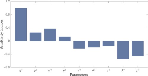
Figure 3. Numerical results for symptomatic infected populations of various starting sizes at $\gamma =0.85$.

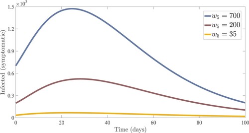
Figure 4. In Ethiopia, EPHI data and numerical results for asymptomatic and symptomatic infected cases from 29 February 2021 to 7 June 2021.

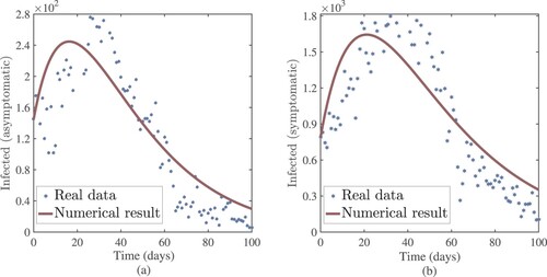
Figure 5. Numerical results for asymptomatic infected people using the Jacobi and Chebyshev spectral collocation methods with $\gamma =0.837$.

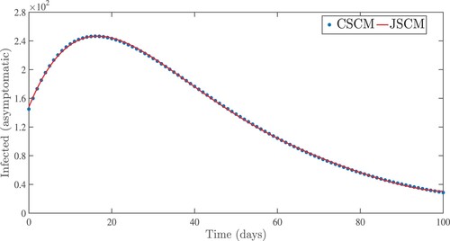
Figure 6. Numerical results for symptomatic infected people using the Jacobi and Chebyshev spectral collocation methods with $\gamma =0.837$.

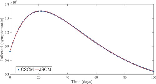
Figure 7. Numerical results for infected people in home-based and isolation programs (HBIC) using the Jacobi and Chebyshev spectral collocation methods with $\gamma =0.837$.

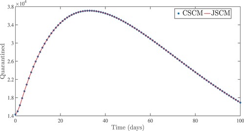
Figure 8. Numerical results for infected patients in treatment centres using the Jacobi and Chebyshev spectral collocation methods with $\gamma =0.837$.

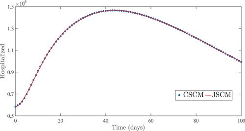
Figure 9. Numerical results for the severe cases using the Jacobi and Chebyshev spectral collocation methods with $\gamma =0.837$.

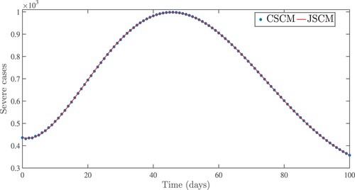
Figure 10. Effects of fundamental reproduction number ${\mathfrak{R}}_0$ on asymptomatic and symptomatic infected cases approximate solutions.

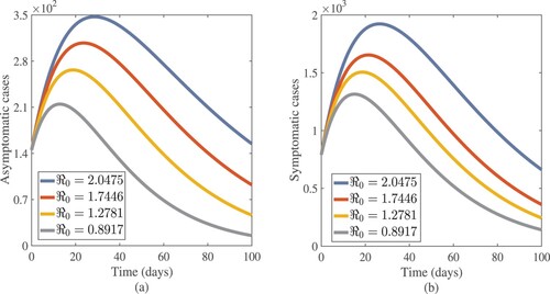
Figure 11. Effects of fundamental reproduction number ${\mathfrak{R}}_0$ on susceptible and quarantined cases approximate solutions.

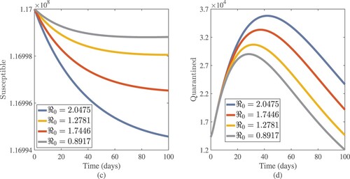
Figure 12. Asymptomatic and symptomatic cases approximate solutions with different values of γ.

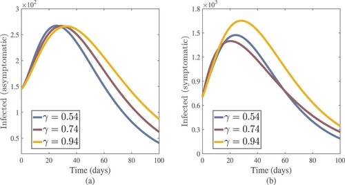
Figure 13. Numerical results of susceptible and hospitalized (active cases treated in hospitals) with different values of γ.

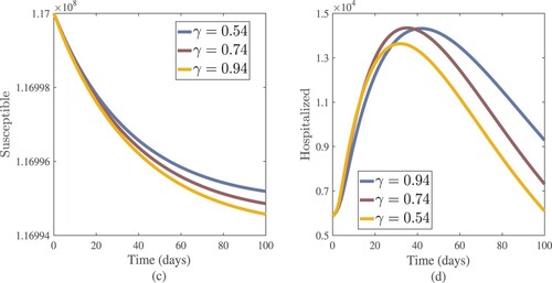
Figure 14. Quarantined and severe cases approximate results with different values of γ.

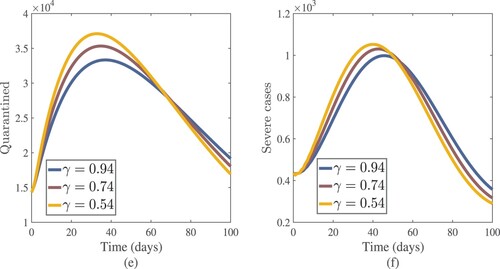
Figure 15. Asymptomatic and symptomatic cases approximate results with increasing values of their treatment rates θ and λ respectively.

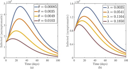
Figure 16. Asymptomatic and symptomatic cases approximate results with increasing values of transmission rate η.

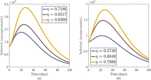
Figure 17. The fundamental reproduction number in relation to the transmission rate η and treatment rate λ.

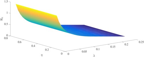
Table 1. The values of model parameters in Equation (17(17) $\begin{array}{l}{}_0^{ABC}{D}_t^{\gamma }S\left(t\right)={\vartheta }^{\gamma }-(\mathrm{\Lambda }+{\omega }^{\gamma })S\\ {}_0^{ABC}{D}_t^{\gamma }E\left(t\right)=\mathrm{\Lambda }S-({\xi }^{\gamma }+{\alpha }^{\gamma }(1-{\xi }^{\gamma })+{\omega }^{\gamma })E\\ {}_0^{ABC}{D}_t^{\gamma }L\left(t\right)={\alpha }^{\gamma }(1-{\xi }^{\gamma })E-({\delta }^{\gamma }+{\tau }^{\gamma }(1-{\delta }^{\gamma })+{\omega }^{\gamma })L\\ {}_0^{ABC}{D}_t^{\gamma }A\left(t\right)={\tau }^{\gamma }(1-{\delta }^{\gamma })L-({\theta }^{\gamma }+{\sigma }^{\gamma }(1-{\theta }^{\gamma })+{\omega }^{\gamma }+a^{\gamma })A\\ {}_0^{ABC}{D}_t^{\gamma }I\left(t\right)={\xi }^{\gamma }E+{\delta }^{\gamma }L-({\lambda }^{\gamma }+{\phi }^{\gamma }(1-{\lambda }^{\gamma })+{\omega }^{\gamma }+b^{\gamma })I\\ {}_0^{ABC}{D}_t^{\gamma }Q\left(t\right)={\phi }^{\gamma }(1-{\lambda }^{\gamma })I-({\nu }^{\gamma }+{\varphi }^{\gamma }(1-{\nu }^{\gamma })+{\omega }^{\gamma }+c^{\gamma })Q\\ {}_0^{ABC}{D}_t^{\gamma }H\left(t\right)={\theta }^{\gamma }A+{\lambda }^{\gamma }I+{\nu }^{\gamma }Q-({\pi }^{\gamma }+{\rho }^{\gamma }(1-{\pi }^{\gamma })+{\omega }^{\gamma }+d^{\gamma })H\\ {}_0^{ABC}{D}_t^{\gamma }C\left(t\right)={\pi }^{\gamma }H-({\psi }^{\gamma }+{\omega }^{\gamma }+e^{\gamma })C\\ {}_0^{ABC}{D}_t^{\gamma }R\left(t\right)={\sigma }^{\gamma }(1-{\theta }^{\gamma })A+{\varphi }^{\gamma }(1-{\nu }^{\gamma })Q+{\rho }^{\gamma }(1-{\pi }^{\gamma })H+{\psi }^{\gamma }C-{\omega }^{\gamma }R\end{array}\}$(17) ) corresponds to the Ethiopian case at $\gamma =0.85$.

Parameter	Value $\left(\frac{1}{\mathrm{d}\mathrm{a}\mathrm{y}}\right)$	Source	Parameter	Value $\left(\frac{1}{\mathrm{d}\mathrm{a}\mathrm{y}}\right)$	Source
ϑ	21,050	Estimated	θ	0.0023	Fitted
ω	$6.78\times {10}^{-6}$	Estimated	b	0.0018	Assumed
η	0.7223	Fitted	σ	0.0225	Fitted
℘	0.0148	Fitted	ν	0.0131	Fitted
ξ	0.0196	Fitted	ϕ	0.0200	Fitted
α	$9.5077\times {10}^{-4}$	Fitted	c	$4.2920\times {10}^{-6}$	Assumed
δ	0.0208	Fitted	π	0.0043	Fitted
τ	0.0010	Fitted	ρ	0.0039	Fitted
λ	0.0038	Fitted	d	$8.0193\times {10}^{-5}$	Assumed
a	0.0018	Assumed	ψ	0.0594	Fitted
φ	0.0103	Fitted	e	0.0121	Assumed

The basic reproduction number (${\mathfrak{R}}_0=1.4331>1$) for the specified model in Equation (17(17) $\begin{array}{l}{}_0^{ABC}{D}_t^{\gamma }S\left(t\right)={\vartheta }^{\gamma }-(\mathrm{\Lambda }+{\omega }^{\gamma })S\\ {}_0^{ABC}{D}_t^{\gamma }E\left(t\right)=\mathrm{\Lambda }S-({\xi }^{\gamma }+{\alpha }^{\gamma }(1-{\xi }^{\gamma })+{\omega }^{\gamma })E\\ {}_0^{ABC}{D}_t^{\gamma }L\left(t\right)={\alpha }^{\gamma }(1-{\xi }^{\gamma })E-({\delta }^{\gamma }+{\tau }^{\gamma }(1-{\delta }^{\gamma })+{\omega }^{\gamma })L\\ {}_0^{ABC}{D}_t^{\gamma }A\left(t\right)={\tau }^{\gamma }(1-{\delta }^{\gamma })L-({\theta }^{\gamma }+{\sigma }^{\gamma }(1-{\theta }^{\gamma })+{\omega }^{\gamma }+a^{\gamma })A\\ {}_0^{ABC}{D}_t^{\gamma }I\left(t\right)={\xi }^{\gamma }E+{\delta }^{\gamma }L-({\lambda }^{\gamma }+{\phi }^{\gamma }(1-{\lambda }^{\gamma })+{\omega }^{\gamma }+b^{\gamma })I\\ {}_0^{ABC}{D}_t^{\gamma }Q\left(t\right)={\phi }^{\gamma }(1-{\lambda }^{\gamma })I-({\nu }^{\gamma }+{\varphi }^{\gamma }(1-{\nu }^{\gamma })+{\omega }^{\gamma }+c^{\gamma })Q\\ {}_0^{ABC}{D}_t^{\gamma }H\left(t\right)={\theta }^{\gamma }A+{\lambda }^{\gamma }I+{\nu }^{\gamma }Q-({\pi }^{\gamma }+{\rho }^{\gamma }(1-{\pi }^{\gamma })+{\omega }^{\gamma }+d^{\gamma })H\\ {}_0^{ABC}{D}_t^{\gamma }C\left(t\right)={\pi }^{\gamma }H-({\psi }^{\gamma }+{\omega }^{\gamma }+e^{\gamma })C\\ {}_0^{ABC}{D}_t^{\gamma }R\left(t\right)={\sigma }^{\gamma }(1-{\theta }^{\gamma })A+{\varphi }^{\gamma }(1-{\nu }^{\gamma })Q+{\rho }^{\gamma }(1-{\pi }^{\gamma })H+{\psi }^{\gamma }C-{\omega }^{\gamma }R\end{array}\}$(17) ) was determined using Table 1, which provides an unstable COVID-19 free equilibrium point and a stable infectious equilibrium point. The fundamental reproduction number, ${\mathfrak{R}}_0>1$, indicates that one COVID-19 infectious person causes the infection of more than one new person. Therefore, the spread of the coronavirus continues. As a result, we advised everyone in charge to fully participate in lowering the value of the fundamental reproduction number to less than one. Virus transmission in the population must be reduced in order to control the disease. Asymptomatic patients are the primary cause of the coronavirus outbreak becoming a pandemic. As a result, increasing the performance of testing the population is a good way to limit virus transmission. Early lockdown of exposed people could be a good control technique against the virus's transmission since it minimizes the danger of coronavirus due to asymptomatic cases. Interaction between susceptible and infectious people will be restricted, and contact will be reduced once infected individuals have been identified, quarantined, and hospitalized. In the absence of a vaccine, we recommend that lockdown, quarantine, and hospitalization are optimal to keep the virus from spreading. Throughout the pandemic, the Ethiopian government must make the required effort to ensure that control techniques are used. When used properly, control methods such as hospitalization, lockdown, and quarantine can significantly limit the heavy impacts of the coronavirus while also protecting Ethiopian.

Disclosure statement

No potential conflict of interest was reported by the author(s).

Data availability statement

We are using data reports from the Ethiopian Public Health Institute from 29 February 2021 to 7 June 2021.

References

- Zhu H, Wei L, Niu P. The novel coronavirus outbreak in Wuhan, China. Global Health Research Policy. 2020;5:6.
- World Health Organization, WHO characterizes Covid-19 as a pandemic, 2020. Available from: https://www.who.int/emergencies/diseases/novel-coronavirus-2019/situation-reports.
- World Health Organization (WHO), Advice for Public., Archived from the original on 26 January 2020 [cited 2020 Feb 10].
- U.S. Centers for Disease Control and Prevention (CDC), Coronavirus Disease 2019 (COVID-19): prevention and treatment. Archived from the original on March 11, 2020 [cited 2020 Mar 11].
- Mwalili S, Kimathi M, Ojiambo V, et al. SEIR model for COVID-19 dynamics incorporating the environment and social distancing. BMC Notes. 2020;13:352. Nairobi, Kenya.
- Kejela T. Probable factors contributing to the fast spread of the novel coronavirus (COVID-19) in Ethiopia. J Infect Dis Epidemiol. 2020;6:169. DOI:10.23937/2474-3658/1510169
- Rajagopal K, Hasanzadeh N, Parastesh F, et al. A fractional-order model for the novel coronavirus (COVID-19) outbreak. Nonlinear Dyn Springer Nature B V. 2020;101:711–718. DOI:10.1007/s11071-020-05757-6
- Baleanu D, Abadi MH, Jajarmi A, et al. A new comparative study on the general fractional model of COVID-19 with isolation and quarantine effects. Alex Eng J. 2022;61:4779–4791. DOI:10.1016/j.aej.2021.10.030
- Allegretti S, Bulai IM, Marino R, et al. Vaccination effect conjoint to fraction of avoided contacts for a sars-Cov-2 mathematical model. Math Model Numer Simul with Appl. 2021;1(2):56–66. DOI:10.53391/mmnsa.2021.01.006
- Ikram R, Khan A, Zahri M, et al. Extinction and stationary distribution of a stochastic COVID-19 epidemic model with time-delay. Comput Biol Med. 2022;141:1–11. Article Id 105115. DOI:10.1016/j.compbiomed.2021.105115
- Youssef H, Alghamdi N, Ezzat MA, et al. A New Dynamical Modelling of the epidemic disease to assessing the rates of spread of COVID-19 in Saudi Arabia: SEIRQ Model, Research Square, 2020.
- Mwalili S, Kimathi M, Ojiambo V, et al. SEIR model for COVID-19 dynamics incorporating the environment and social distancing. BMC Res Notes. 2020;13:352.
- Khan MA, Atangana A. Modeling the dynamics of novel coronavirus (2019-nCov) with fractional derivative. Alex Eng J. 2020;59(4):2379–2389. DOI:10.1016/j.aej.2020.02.033
- Ahmed I, Baba IA, Yusuf A, et al. Analysis of Caputo fractional-order model for COVID-19 with lockdown. Adv Differ Equ. 2020;2020:394.
- Jajarmi A, Baleanu D, Vahid KZ, et al. A general fractional formulation and tracking control for immunogenic tumor dynamics. Math Meth Appl Sci. 2022;45:667–680. DOI:10.1002/mma.7804
- Özköse F, Yılmaz S, Yavuz M, et al. A fractional modeling of tumor–immune system interaction related to lung cancer with real data. Eur Phys J Plus. 2022;137:40. DOI:10.1140/epjp/s13360-021-02254-6
- Moore EJ, Sirisubtawee S, Koonprasert S. A Caputo–Fabrizio fractional differential equation model for HIV/AIDS with treatment compartment. Adv Differ Equ. 2019;2019:200. DOI:10.1186/s13662-019-2138-9
- Alqahtani RT. Atangana-Baleanu derivative with fractional order applied to the model of groundwater within an unconfined aquifer. J Nonlinear Sci Appl. 2016;9:3647–3654. Available from: www.tjnsa.com.
- Deressa CT, Duressa GF. Analysis of Atangana Baleanu fractional order SEAIR epidemic model with optimal control. Adv Differ Equ. 2021;2021:174. DOI:10.1186/s13662-021-03334-8
- Uçar S. Analysis of a basic SEIRA model with Atangana-Baleanu derivative. AIMS Math. 2020;5(2):1411–1424. DOI:10.3934/math.2020097
- Suthar DL, Habenom H, Aychluh M. Effect of vaccination on the transmission dynamics of COVID-19 in Ethiopia. Results Phys. 2022;32:1–11. Article Id 105022. DOI:10.1016/j.rinp.2021.105022
- Habenom H, Aychluh M, Suthar DL, et al. Modeling and analysis on the transmission of covid-19 pandemic in Ethiopia. Alex Eng J. 2022;61:5323–5342. DOI:10.1016/j.aej.2021.10.054
- Jajarmi A, Baleanu D, Vahid KZ, et al. A new and general fractional Lagrangian approach: A capacitor microphone case study. Results Phys. 2021;31:1–8. Article Id 104950. DOI:10.1016/j.rinp.2021.104950
- Habenom H, Suthar DL, Baleanu D, et al. A numerical simulation on the effect of vaccination and treatments for the fractional hepatitis B model. J Comput Nonlinear Dyn. 2021;16:1–6. DOI:10.1115/1.4048475
- Din A, Abidin MZ. Analysis of fractional-order vaccinated hepatitis-B epidemic model with mittag-Leffler kernels. Math Model Numer Simul With Appl. 2022;2(2):59–72. DOI:10.53391/mmnsa.2022.006
- Naik PA, Eskandari Z, Yavuz M, et al. Complex dynamics of a discrete-time Bazykin–Berezovskaya prey-predator model with a strong Allee effect. J Comput Appl Math. 2022;413:1–12. Article Id 114401. DOI:10.1016/j.cam.2022.114401
- Bonyah E, Yavuz M, Baleanu D, et al. A robust study on the listeriosis disease by adopting fractal-fractional operators. Alex Eng J. 2022;61(3):2016–2028. DOI:10.1016/j.aej.2021.07.010
- Hammouch Z, Yavuz M, Özdemi N. Numerical solutions and synchronization of a variable-order fractional chaotic system. Math Model Numer Simul With Appl. 2021;1(1):11–23.
- Joshi H, Jha BK. Chaos of calcium diffusion in Parkinson's infectious disease model and treatment mechanism via hilfer fractional derivative. Math Model Numer Simul With Appl. 2021;1(2):84–94. DOI:10.53391/mmnsa.2021.01.008
- Naik PA, Owolabi KM, Yavuz M, et al. Chaotic dynamics of a fractional order HIV-1 model involving AIDS-related cancer cells. Chaos Solitons Fractals. 2020;140:1–13. Article Id 110272. DOI:10.1016/j.chaos.2020.110272
- Shiralashetti SC, Deshi AB, Mutalik Desai PB. Haar wavelet collocation method for the numerical solution of singular initial value problems. Ain Shams Eng J. 2016;7:663–670. DOI:10.106/j.asej.2015.06.006
- Mahdy AMS, El-dahdouh AAA. Numerical simulation for the approximating of given up smoking model in fractional order. Int J Appl Eng Res. 2019;14(2):589–593.
- Atangana A, araz SI. A novel covid-19 model with fractional differential operators with singular and non-singular kernels: analysis and numerical scheme based on Newton polynomial. Alex Eng J. 2021;60:3781–3806. DOI:10.1016/j.aej.2021.02.016
- Gebremeskel AA, Berhe HW, Atsbaha HA. Mathematical modelling and analysis of COVID-19 epidemic and predicting its future situation in Ethiopia. Results Phys. 2021;22:1–10. Article Id 103853. DOI:10.1016/j.rinp.2021.103853
- Omar OAM, Elbarkouky RA, Ahmed HM. Fractional stochastic models for COVID-19: case study of Egypt. Results Phys. 2021;23:1–7. Article Id 104018. DOI:10.1016/j.rinp.2021.104018
- Peter OJ, Qureshi S, Yusuf A, et al. A new mathematical model of COVID-19 using real data from Pakistan. Results Phys. 2021;24:1–10. Article Id 104098. DOI:10.1016/j.rinp.2021.104098
- Okuonghae D, Omame A. Analysis of a mathematical model for COVID-19 population dynamics in Lagos, Nigeria. Chaos Solitons Fract. 2020;139:1–18. Article Id 110032. DOI:10.1016/j.chaos.2020.110032
- Özköse F, Yavuz M, Şenel MT, et al. Fractional order modelling of omicron SARS-CoV-2 variant containing heart attack effect using real data from the United Kingdom. Chaos Solitons Fractals. 2022;157:1–24. Article Id 111954. DOI:10.1016/j.chaos.2022.111954
- Özköse F, Yavuz M. Investigation of interactions between COVID-19 and diabetes with hereditary traits using real data: a case study in Turkey. Comput Biol Med. 2022;141:1–22. Article Id 105044. DOI:10.1016/j.compbiomed.2021.105044
- Yavuz M, Coşar FÖ, Günay F, et al. A new mathematical modeling of the COVID-19 pandemic including the vaccination campaign. Open J Model Simul. 2021;9:299–321. DOI:10.4236/ojmsi.2021.93020
- Abdo MS, Shah K, Wahash HA, et al. On a comprehensive model of the novel coronavirus (COVID-19) under Mittag-Leffler derivative. Chaos Solitons Fractals. 2020;135:1–15. Article Id 109867.
- Atangana A, Baleanu D. New fractional derivatives with nonlocal and non-singular kernel: theory and application to heat transfer model. Therm Sci. 2016;20:763–769.
- Saad KM, Khader MM, Gomez-Aguilar JF, et al. Numerical solutions of the fractional fisher's type equations with Atangana-Baleanu fractional derivative by using spectral collocation methods. Interdiscip J Nonlinear Sci. 2019;29:1–10.
- Alqahtani RT. Atangana-Baleanu derivative with fractional order applied to the model of groundwater within an unconfined aquifer. J Nonlinear Sci Appl. 2016;9:3647–3654.
- Canuto C, Hussaini MY, Quarteroni A, et al. Spectral methods: fundamentals in single domain. New York: Springer; 2006.
- Baleanu D, Fernandez A. On some new properties of fractional derivatives with Mittag-Leffler kernel. Commun Nonlinear Sci Numer Simul. 2018;59:444–462.
- Ministry of Health-Ethiopia and Ethiopian Public Health Institute, 6 June 2021. Available from: http://www.ephi.gov.et and https://www.worldometers.info.