Applications of Elzaki decomposition method to fractional relaxation-oscillation and fractional biological population equations

Abstract

Elzaki decomposition method (EDM) is adopted to deal with the fractional-order relaxation and damped oscillation equation along with time-fractional spatial diffusion biological population model in different suitable habitat situations. In accordance with the graphs for the solutions obtained, the fractional relaxation exhibits super-slow phenomenon due to its extended descent, and fractional damped oscillation is an intermediate process that explains damped oscillation dynamic systems induced by some attenuated oscillations. The biological population model of time-fractional spatial diffusion depicts a rapid rise in population density in an ecosystem in a suitable habitat that is migrating from an unfavourable zone.

KEYWORDS:

• Elzaki transform
• Adomian decomposition method
• fractional relaxation oscillation equation
• fractional biological population equation

MATHEMATICS SUBJECT CLASSIFICATIONS: 26A33:

• 33E12
• 35A22
• 34C26
• 60J70

1. Introduction

Fractional calculus is used to analyse, acclimate and implement more efficient and capable systems in numerous real-world fields, like economics, physics, life sciences and engineering including financial economy, electromagnetics, viscoelasticity, epidemiological models, diffusion in cell membranes, fluid mechanics, image processing. Because of their memory and heredity concerns, fractional differential equations are best characterized to model physical and biological processes [1,2]. Various analytical and numerical approaches are taken in many research attempts to achieve exact and approximate solutions for fractional-order differential equations.

Elzaki transform introduced in Ref. [3] is itself and with combinations of other techniques is being used for solving various classical and fractional, linear and non-linear, ordinary and partial differential equations describing various physical and biological process. In Ref. [4], the Elzaki transform is used to solve partial differential equations, whereas in Ref. [5] it is used to solve non-linear partial differential equations of fractional order. In Ref. [6], the Homotopy perturbation method with Elzaki transform is used to solve a system of non-linear partial differential equations. In Ref. [7], the Elzaki transformed method is used to provide an analytical solution of a linear fractionally damped oscillator. In Ref. [8], the radial diffusivity and shock wave equations are solved using the Elzaki variational iteration method, and in Ref. [9], a numerical method based on the Elzaki transform and He’s Homotopy perturbation method (HPM) is developed for solving non-linear partial differential equations arising in spatial flow that characterize the general biological population.

The Elzaki decomposition method (EDM), which is a combination of the Elzaki transform and the Adomian decomposition method first developed in Ref. [10]. EDM is a straightforward and practical approach for solving both linear and non-linear differential equations. It is highly recommended to solve linear and non-linear differential equation with shorten calculation part as compared to other methods.

In this work, firstly the EDM is applied to fractional relaxation and damped oscillation equations with a Caputo fractional derivative of order $\alpha$ with $0<\alpha \le 1$ and $1<\alpha \le 2$, respectively, to find analytic solution involving Mittag–Leffler function. The plots for different values of $\alpha$ are analysed for the solutions obtained. After that, application of EDM is adopted to solve and analyse time-fractional spatial diffusion biological population model for both Malthusian law and Verhulst law in suitable habitat situations from various unfavourable zones.

2. Preliminaries

The Elzaki transform of a function $g\left(t\right)ϵA,\mathrm{\forall }t\ge 0,$ is defined by the integral [3] (2.1) $E\left[g\right(t);v]=G\left(v\right)=v\underset{0}{\overset{t}{\int }}g\left(t\right)e^{-\frac{t}{v}}dt,k_1<v<k_2,$(2.1) where $A=\left\{g\left(t\right):\mathrm{\exists }M,k_1,k_2>0,|g\left(t\right)|<M{e}^{\frac{|t|}{k_j}},tϵ{(-1)}^j\times \left[0,\mathrm{\infty }\right)\right\},$ M being finite constant and $k_1,k_2$ being finite or infinite.

The inverse of Elzaki transform is denoted by $E^{-1}\left[G\left(v\right);t\right]=g\left(t\right),t>0$.

ELzaki transform of the power series function is [3] given by (2.2) $E\left[\sum _{m=0}^{\mathrm{\infty }}{a}_m{t}^m;v\right]=\sum _{m=0}^{\mathrm{\infty }}m!a_m{v}^{m+2}.$(2.2) Also, for any $\alpha \in \mathbb{R}$ (2.3) $E\left[t^{\alpha };v\right]=\mathrm{\Gamma }(\alpha +1)v^{\alpha +2}.$(2.3) The Elzaki transform of Caputo fractional derivative of a function is given by [5] (2.4) $E\left[{}_C{D}_{0^{+}}^{\alpha }g\left(t\right);v\right]=\frac{G\left(v\right)}{v^{\alpha }}-\sum _{m=0}^{n-1}{v}^{m-\alpha +2}{\text{g}}^{\left(m\right)}\left(0\right)\text{, }n-1<\alpha \le n.$(2.4)

3. Fractional relaxation oscillation equation

In physical, chemical and biological processes, an oscillator is something that exhibits a rhythmic periodic reaction. Many real mechanical, radio-technical, biological and other things have oscillatory processes in which a slow smooth transition of an object’s status over a finite length of time shifts to an irregular change of status over an incredibly short period. The behaviour of a physical system returning to equilibrium after being disrupted provides the basis for a relaxation oscillation. A damped oscillating system is an oscillator that fades away over time owing to energy loss, such as a swinging pendulum, a weight on a spring or a resistor-inductor-capacitor circuit. Relaxation and damped oscillations are described by ordinary differential equations of order one and two, respectively.

In fractional oscillators, the amplitude of the oscillation decays. Because the fractional oscillator is accompanied by a damping mechanism [11], total energy in physical systems dissipates. A comprehensive survey of recent work in the subject of fractional calculus application to dynamic solid mechanics problems is provided in Ref. [12]. We present a fractional differentiation-based model of relaxation and damped oscillation that is more relevant for the physical nature of diverse oscillatory processes with damping.

In order to investigate the mechanical behaviour of objects fractional-order derivatives are preferably applicable in place of classical integer-order. In the relaxation and oscillation models, fractional derivatives are used to for accurate modelling of super-slow relaxation and damped oscillation dynamic systems that require accurate modelling as [13]: (3.1) $\begin{array}{l}{}_C{D}_t^{\alpha }g\left(t\right)+\lambda g\left(t\right)=f\left(t\right),t>0,\\ g\left(0\right)=a\text{ if}0<\alpha \le 1,\\ or\\ g\left(0\right)=b,g^{\left(1\right)}\left(0\right)=c\text{if}1<\alpha \le 2,\end{array}$(3.1) where $\lambda$ is a constant that is not negative. For $0<\alpha \le 2$, this Equation (3.1) is known as the fractional relaxation oscillation equation. Which is generated by replacing the first and second-order time derivatives in the related classical relaxation and damped oscillation equations with a Caputo fractional derivative of order $\alpha$ with $0<\alpha \le 1$ and $1<\alpha \le 2$ correspondingly.

3.1. Elzaki decomposition method on fractional relaxation oscillation equation

For a field variable function $g\left(t\right)$ and a given continuous function $f\left(t\right)$ with t ≥ 0, we consider the fractional relaxation oscillation differential equation of order $\alpha \left(n-1<\alpha \le n\right)$ as [13]: (3.2) ${}_C{D}_t^{\alpha }g\left(t\right)+\lambda g\left(t\right)=f\left(t\right),t>0,$(3.2) (3.3) $\text{with initial conditions}{g}^{\left(m\right)}\left(0^{+}\right)=a_m,m=0,1,2,\dots n-1.$(3.3) where $\lambda$ is a positive constant and ${}_C{D}_t^{\alpha }$ denotes Caputo fractional derivative of order $\alpha$.

On taking the Elzaki transform of (3.2) by using (2.4), subject to the initial condition (3.3), we have (3.4) $E\left[g\left(t\right);v\right]=\sum _{m=0}^{n-1}{v}^{m+2}{a}_m-v^{\alpha }E\left[\lambda g\left(t\right)-f\left(t\right);v\right].$(3.4) On applying Elzaki inverse transform on (3.4) and decomposing as $g\left(t\right)=\sum _{k=0}^{\mathrm{\infty }}{g}_k\left(t\right)$, we have (3.5) $g\left(t\right)=\sum _{k=0}^{\mathrm{\infty }}{g}_k\left(t\right)=E^{-1}\left[\sum _{m=0}^{n-1}{v}^{m+2}{a}_m-v^{\alpha }E\left[\lambda \sum _{k=0}^{\mathrm{\infty }}{g}_k\left(t\right)-f\left(t\right);v\right]\right]$(3.5) Applying the Adomian decomposition method, the components of $g\left(t\right)$ using (2.2), recursively be obtained by (3.6) $\begin{array}{rl}{g}_0\left(t\right)& =E^{-1}\left[\sum _{m=0}^{n-1}{v}^{m+2}{a}_m+v^{\alpha }E\left[f\left(t\right);v\right];t\right]=\sum _{m=0}^{n-1}{a}_m\frac{t^m}{m!}+E^{-1}\left[v^{\alpha }E\left[f\left(t\right);v\right];t\right],\end{array}$(3.6) (3.7) $\begin{array}{rl}\text{and}{g}_{k+1}\left(t\right)& =-E^{-1}\left[v^{\alpha }E\left[\lambda g_k\left(t\right);v\right];t\right].\end{array}$(3.7) The components $g_0,g_1,g_2,\dots ,g_n$ can be obtained when the Elzaki Transform and the Elzaki inverse transform are applied to (3.6) and (3.7) while taking some particular continuous function $f\left(t\right)$, resulting the general solution $g\left(t\right)$ as $g\left(t\right)=g_0\left(t\right)+g_1\left(t\right)+g_2\left(t\right)+\cdots .$ In particular, if we take $0<\alpha \le 1,\lambda ={\omega }^{\alpha },f\left(t\right)=0\text{ and g}\left(0^{+}\right)=a$ in (3.2) and (3.3), we arrive at

Problem 3.1: Consider the following fractional relaxation oscillation differential equation (3.8) ${}_C{D}_t^{\alpha }g\left(t\right)+{\omega }^{\alpha }g\left(t\right)=0,g\left(0^{+}\right)=a,t>0,0<\alpha \le 1.$(3.8) Solution: In view of (3.6) and (3.7), here we have (3.9) $g_0\left(t\right)=a\text{and}{g}_{k+1}\left(t\right)=-E^{-1}\left[v^{\alpha }E\left[{\omega }^{\alpha }{g}_k\left(t\right);v\right];t\right],$(3.9) which gives the solution for (3.8), on using (2.3) as (3.10) $g\left(t\right)=a-a\frac{{\omega }^{\alpha }{t}^{\alpha }}{\mathrm{\Gamma }\left(\alpha +1\right)}+\frac{{\omega }^{2\alpha }{t}^{2\alpha }}{\mathrm{\Gamma }\left(2\alpha +1\right)}-\cdots =a\sum _{k=0}^{\mathrm{\infty }}(-1{)}^k\frac{{\omega }^{k\alpha }{t}^{k\alpha }}{\mathrm{\Gamma }\left(k\alpha +1\right)}=a{E}_{\alpha }\left[-{\left(\omega t\right)}^{\alpha }\right],$(3.10) where $E_{\alpha }$, denotes the Mittag–Leffler function [14].

For the sake of convenience, we will set $a=1$ and $\omega =1$ to show graphs of the solution (3.10) of fractional relaxation oscillation differential Equation (3.8) in Figure 1, without losing generality.

Figure 1. Graph of the solution of fractional relaxation oscillation differential equation for different values of $\alpha$.

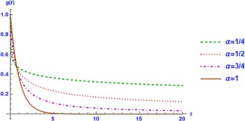
The solution $E_{\alpha }\left(-t^{\alpha }\right)$ of the fractional relaxation Equation (3.10) decays significantly more slowly than the solution $exp\left(-t\right)$ of the classical relaxation equation ($\alpha =1$).Because of its protracted fall, fractional relaxation is often characterized as a super-slow phenomenon.

Next, if we take $1<\alpha \le 2,\lambda ={\omega }^{\alpha },f\left(t\right)=0\text{ and g}\left(0^{+}\right)=a,{\text{g}}^{\left(1\right)}\left(0^{+}\right)=b$ in (3.2) and (3.3), we reach at

Problem 3.2: Consider the following damped oscillation fractional differential equation as follow: (3.11) ${}_C{D}_t^{\alpha }g\left(t\right)+{\omega }^{\alpha }g\left(t\right)=0,g\left(0^{+}\right)=a,g^{\left(1\right)}\left(0^{+}\right)=b,t>0,1<\alpha \le 2.$(3.11) In view of (3.6) and (3.7), here we have (3.12) $g_0\left(t\right)=a+bt\text{and}{g}_{k+1}\left(t\right)=-E^{-1}\left[v^{\alpha }E\left[{\omega }^{\alpha }{g}_k\left(t\right);v\right];t\right].$(3.12) The components $g_1,g_2,\dots$ are obtained as $\begin{array}{rl}{g}_1\left(t\right)& =-E^{-1}\left[v^{\alpha }E\left[{\omega }^{\alpha }{g}_0\left(t\right);v\right];t\right]=-E^{-1}\left[v^{\alpha }E\left[{\omega }^{\alpha }(a+bt);v\right];t\right]\\ & =-\frac{a{\omega }^{\alpha }{t}^{\alpha }}{\mathrm{\Gamma }\left(\alpha +1\right)}-\frac{b{\omega }^{\alpha }{t}^{\alpha +1}}{\mathrm{\Gamma }\left(\alpha +2\right)},\\ g_2\left(t\right)& =-E^{-1}\left[v^{\alpha }E\left[{\omega }^{\alpha }{g}_1\left(t\right);v\right];t\right]\\ & =E^{-1}\left[v^{\alpha }E\left[-\frac{a{\omega }^{2\alpha }{t}^{\alpha }}{\mathrm{\Gamma }\left(\alpha +1\right)}-\frac{b{\omega }^{2\alpha }{t}^{\alpha +1}}{\mathrm{\Gamma }\left(\alpha +2\right)};v\right];t\right]=\frac{a{\omega }^{2\alpha }{t}^{2\alpha }}{\mathrm{\Gamma }\left(2\alpha +1\right)}+\frac{b{\omega }^{2\alpha }{t}^{2\alpha +1}}{\mathrm{\Gamma }\left(2\alpha +2\right)}.\end{array}$

Resulting in the general solution of (3.11) as (3.13) $\begin{array}{l}\begin{array}{l}g\left(t\right)=a+bt-{\displaystyle \frac{a{\omega }^{\alpha }{t}^{\alpha }}{\mathrm{\Gamma }\left(\alpha +1\right)}}-{\displaystyle \frac{b{\omega }^{\alpha }{t}^{\alpha +1}}{\mathrm{\Gamma }\left(\alpha +2\right)}}+{\displaystyle \frac{a{\omega }^{2\alpha }{t}^{2\alpha }}{\mathrm{\Gamma }\left(2\alpha +1\right)}}+{\displaystyle \frac{b{\omega }^{2\alpha }{t}^{2\alpha +1}}{\mathrm{\Gamma }\left(2\alpha +2\right)}}+\cdots \\ =a\sum _{k=0}^{\mathrm{\infty }}(-1{)}^k{\displaystyle \frac{{\omega }^{k\alpha }{t}^{k\alpha }}{\mathrm{\Gamma }\left(k\alpha +1\right)}}+b\sum _{k=0}^{\mathrm{\infty }}(-1{)}^k\frac{{\omega }^{k\alpha }{t}^{k\alpha +1}}{\mathrm{\Gamma }\left(k\alpha +2\right)}=a{E}_{\alpha }\left[-{\left(\omega t\right)}^{\alpha }\right]+bt{E}_{\alpha ,2}\left[-{\left(\omega t\right)}^{\alpha }\right].\end{array}\end{array}$(3.13) where $E_{\alpha }$ and $E_{\alpha ,\text{β}}$ denote the Mittag–Leffler functions [14,15]. This solution (3.13) is same as the solution obtained by Achar et al. [16] by using Laplace transform method in solving integral equation of motion of harmonic oscillator.

Again, for convenience, we will set $a=1,b=1$ and $\omega =1$ to show graphs of the solution (3.13) of damped oscillation fractional differential Equation (3.11) in Figure 2, without losing generality.

Figure 2. Graph of the solution of damped oscillation fractional differential equation for different values of $\alpha$.

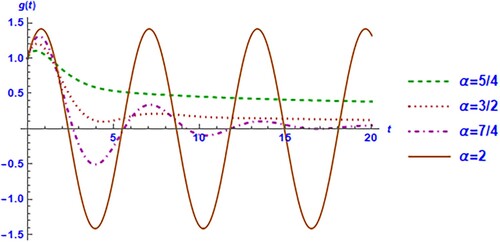
The solution of damped oscillation fractional $\left(1<\alpha \le 2\right)$ differential equation $\begin{array}{l}{E}_{\alpha }\left[-t^{\alpha }\right]+t{E}_{\alpha ,2}\left[-t^{\alpha }\right]\end{array}$ demonstrates asymptotic algebraic decay rather than permanent oscillations, in contrast to the solution of classical oscillation $\alpha =2$ equation $\cos t+\sin t$. Only some attenuated oscillations appear as a temporary condition in the fractional solution, with their number and initial amplitude increasing with $\alpha$. Because of the presence of intermediate components, fractional oscillations are usually referred to as an intermediate process.

4. Fractional biological population equation

Population growth, which is one of the world’s primary issues, is influenced by a variety of biological and non-biological variables. Globalization, which is a sort of geographical diffusion, is causing population to expand at an alarming rate. The spread of diseases has been accelerated by worldwide migration, but global advancements in public health, medical and family planning technology have played a critical role in global increases in life expectancy [17–19]. To better understand how dispersal impacts species evolution, population dynamics and distribution, mathematical biologists typically use models in which movement is represented by a spatial diffusion process [20,21].

A proliferation of a phenomenon that has a source and diffuses outwards through space and time from constrained sources, such as the spread of a fire or pollution, is known as spatial diffusion. Reference [22] demonstrated the conceptual applicability of the spatial diffusion process to represent redistribution of species in space due to random migration of individuals for any population density.

The spatial diffusion of the population is based on the premise of dispersal based on the irregular motion of each individual in a biological population [23]. Mathematical model of spatial diffusion can be used in a variety of settings, including innovation acceptance, cultural development, epidemiology, settlement, migration and landscape evolution [24,25]. Diffusion systems-based mathematical modelling of biological populations, with applications in ecology, epidemiology and neural systems are focused in Ref. [26].

In recent research, the concept of fractional generalization has been demonstrated to be a successful technique for modelling a variety of natural events. Various fractional diffusion models have been developed to predict the human brain’s response to external stimuli [27], the role of structural heterogeneity in repolarization dispersion in cardiac electrical propagation [28], charge transfer in dye-sensitized solar cells [29], dust aerosols floating in Mars’ atmosphere that cause attenuation of solar radiation traversing the atmosphere [30], and fluid transport through porous media [31], impact on raise of environmental pollution and occurrence in biological populations by presenting a mathematical model relating to incomplete H-function [32] and many others. In these models, fractional derivatives have been incorporated into partial differential equations, allowing for the description of anomalous diffusion within fractal spaces.

The non-linear partial differential Equation (4.1) describes the spatial diffusion model of biological population in a region $R$ based on the classical model given by Skellam [20] (4.1) $\frac{\mathrm{\partial }\rho }{\mathrm{\partial }t}=\left(\frac{{\mathrm{\partial }}^2}{\mathrm{\partial }{x}^2}+\frac{{\mathrm{\partial }}^2}{\mathrm{\partial }{y}^2}+\frac{{\mathrm{\partial }}^2}{\mathrm{\partial }{z}^2}\right)\phi \left(\rho \right)+\sigma \left(\rho \right),$(4.1) where $\rho (\mathbf{x},t)$ is the population density, that provides the overall population at a given period by integrating the number of inhabitants per unit volume throughout the region $R$. The population supply $\sigma (\mathbf{x},t)$ is a non-linear function of $x$ and $t$, expresses the rate at which inhabitants are added to the population (per unit volume) through births and deaths.

Now, we consider constitutive equations for $\sigma$ as the Malthusian law and Verhulst law given by $\sigma \left(\rho \right)=\mu \rho ,\left(\mu =\text{constant}\right)$ and $\sigma \left(\rho \right)=\mu \rho -\lambda {\rho }^2,\left(\mu ,\lambda =\text{ constant}\right)$, respectively. If $\mu \ge 0$, the entire space is eventually inhabited, regardless of the beginning data; if $\mu <0$, and the population is originally contained within a finite interval, then the population is permanently contained inside a finite interval.

Also, focus on the case $\phi$ has a specific form; this allows us to apply the theory to the case in which several well-known results, such as showing the diffusion velocity of inhabitants at the wave front determines the finite speed of propagation for disturbances moving through unpopulated areas, can be demonstrated. (4.2) $\phi \left(\rho \right)=K{\rho }^{\text{β}},(K>0,\text{β}\ge 1).$(4.2) The partial differential Equation (4.1) will then be reduced to (4.3) $\frac{\mathrm{\partial }\rho }{\mathrm{\partial }t}=K\left(\frac{{\mathrm{\partial }}^2}{\mathrm{\partial }{x}^2}+\frac{{\mathrm{\partial }}^2}{\mathrm{\partial }{y}^2}+\frac{{\mathrm{\partial }}^2}{\mathrm{\partial }{z}^2}\right){\rho }^{\text{β}}+\sigma \left(\rho \right).$(4.3) Now, we suppose that $K=1$ without losing generality; this normalization is simply performed by changing spatial coordinates.

We investigate a Caputo fractional generalization of spatial diffusion model of biological population [21] to simulate genuine movements arising from random scattering of species, which will be relevant to many natural biological circumstances. The initial-value problem under study entails locating a density distribution that satisfies certain conditions, with the underlying region assumed to be the real line R is given by (4.4) $\frac{\mathrm{\partial }\rho }{\mathrm{\partial }t}\left(x,t\right)=D_x^2{\rho }^{\text{β}}\left(x,t\right)+\sigma \left(\rho \left(x,t\right)\right),t\ge 0,x\in \text{R},\text{β}\ge 1,$(4.4) the initial condition: (4.5) $\rho \left(x,0\right)={\rho }_0\left(x\right).$(4.5)

3.2. Elzaki decomposition method on time-fractional biological population equation

Now, by taking fractional generalization of biological population problem given by (4.4) and (4.5) with respect to time, we arrive at the following fractional-order biological population problem (4.6) ${}_C{D}_t^{\alpha }\rho \left(x,t\right)=D_x^2{\rho }^{\text{β}}\left(x,t\right)+\sigma \left(\rho \left(x,t\right)\right),n-1<\alpha \le n,t\ge 0,x\in \text{R},\text{β}\ge 1,$(4.6) the initial condition: (4.7) ${\rho }^{\left(m\right)}\left(x,0\right)={\rho }_m\left(x\right),m=0,1,2,\dots n-1.$(4.7) where ${}_C{D}_t^{\alpha }\rho \left(x,t\right)$ denotes Caputo fractional derivative of order $\alpha$ of population density $\rho (\mathbf{x},t)$ and population supply $\sigma \left(\rho \left(x,t\right)\right)$.

On taking the Elzaki transform of (4.6), by using (2.4) subject to the initial condition (4.7), we have (4.8) $E\left[\rho \left(x,t\right);v\right]=\sum _{m=0}^{n-1}{v}^{m+2}{\rho }_m\left(x\right)+v^{\alpha }E\left[D_x^{\lambda }{\rho }^{\text{β}}\left(x,t\right)+\sigma \left(\rho \left(x,t\right)\right);v\right].$(4.8) On applying Elzaki inverse transform on (4.8) and decomposing as $\rho \left(x,t\right)=\sum _{k=0}^{\mathrm{\infty }}{\rho }_k\left(x,t\right)$, we have (4.9) $\rho \left(x,t\right)=\sum _{k=0}^{\mathrm{\infty }}{\rho }_k\left(x,t\right)=E^{-1}\left[\sum _{m=0}^{n-1}{v}^{m+2}{\rho }_m\left(x\right)+v^{\alpha }E\left[\sum _{k=0}^{\mathrm{\infty }}{A}_k\left(\rho \left(x,t\right)\right);v\right]\right],$(4.9) where $A_k$ represent the Adomian polynomials the non-linear term $E[D_x^{\lambda }{\rho }^{\text{β}}\left(x,t\right)+\sigma (\rho \left(x,t\right));v]$, which

1. for Malthusian law $\sigma \left(\rho \right)=\mu \rho$ is given by (4.10) $\begin{array}{rl}{A}_0& =D_x^2{\rho }_0^{\text{β}}\left(x,t\right)+\mu {\rho }_0\left(x,t\right),\end{array}$(4.10) (4.11) $\begin{array}{rl}{A}_1& =\text{β}{D}_x^2\left({\rho }_0^{\text{β}-1}\left(x,t\right){\rho }_1\left(x,t\right)\right)+\mu {\rho }_1\left(x,t\right),\end{array}$(4.11) (4.12) $\begin{array}{rl}2A_2& =D_x^2\left(\text{β}(\text{β}-1){\rho }_1^2\left(x,t\right){\rho }_0^{\text{β}-2}\left(x,t\right)+2\text{β}{\rho }_0^{\text{β}-1}\left(x,t\right){\rho }_2\left(x,t\right)\right)+\mu {\rho }_2\left(x,t\right),\end{array}$(4.12) and so on,

2. for Verhulst law $\sigma \left(\rho \right)=\mu \rho -\lambda {\rho }^2$ are given by (4.13) $\begin{array}{rl}{A}_0& =D_x^2{\rho }_0^{\text{β}}\left(x,t\right)+\mu {\rho }_0\left(x,t\right)-\lambda {\rho }_0^2\left(x,t\right),\end{array}$(4.13) (4.14) $\begin{array}{rl}{A}_1& =\text{β}{D}_x^2\left({\rho }_0^{\text{β}-1}\left(x,t\right){\rho }_1\left(x,t\right)\right)+\mu {\rho }_1\left(x,t\right)-2\lambda {\rho }_0\left(x,t\right){\rho }_1\left(x,t\right),\end{array}$(4.14) (4.15) $\begin{array}{rl}{A}_2& =D_x^2\left(\frac{\text{β}}{2}(\text{β}-1){\rho }_1^2\left(x,t\right){\rho }_0^{\text{β}-2}\left(x,t\right)+\text{β}{\rho }_0^{\text{β}-1}\left(x,t\right){\rho }_2\left(x,t\right)\right)+\mu {\rho }_2\left(x,t\right)\\ & -\lambda \left({\rho }_1^2\left(x,t\right)+2{\rho }_0\left(x,t\right){\rho }_2\left(x,t\right)\right),\end{array}$(4.15) and so on.

   Identifying the zero component ${\rho }_0\left(x,t\right)$ by ${\rho }^{\left(m\right)}\left(x,0\right)$ and the following recurrence relation will be used to determine the remaining components (4.16) $\begin{array}{rl}{\rho }_0\left(x,t\right)& =E^{-1}\left[\sum _{m=0}^{n-1}{v}^{m+2}{\rho }_m\left(x\right)\right]=\sum _{m=0}^{n-1}{\rho }_m\left(x\right)\frac{t^m}{m!},\end{array}$(4.16) (4.17) $\begin{array}{rl}\text{and}{\rho }_{k+1}\left(x,t\right)& =E^{-1}\left[v^{\alpha }E\left[A_k\left(\rho \left(x,t\right)\right)+\mu {\rho }_k\left(x,t\right);v\right];t\right].\end{array}$(4.17) The components ${\rho }_1,{\rho }_2,\dots ,{\rho }_n$ can be obtained when the Elzaki Transform and its inverse are applied to (4.17), resulting the general solution $\rho \left(x,t\right)$ as $\rho \left(x,t\right)=\sum _{k=0}^{\mathrm{\infty }}{\rho }_k\left(x,t\right)$.

Now by taking $0<\alpha \le 1$ for Malthusian law and $\text{β}=1$ the effect of random dispersal [20], in (4.6) and (4.7), and by considering following two cases.

Case (i): An unfavourable zone that extends endlessly in one direction borders a suitable ecosystem, i.e. $a\le x<\mathrm{\infty },\rho \left(a,t\right)=P,\rho \left(\mathrm{\infty },t\right)=0$.

Case (ii): A suitable habitat surrounds an unfavourable segment on both ends, i.e. $-a\le x<a,\rho \left(-a,t\right)=\rho \left(a,t\right)=P$.

Problem 4.1: We reach at the following fractional model of biological population (4.18) ${}_C{D}_t^{\alpha }\rho \left(x,t\right)=D_x^2\rho \left(x,t\right)+\mu \rho \left(x,t\right),t\ge 0,x\in \text{R,}$(4.18) with initial conditions for the two cases

1. when $a\le x<\mathrm{\infty },\rho \left(a,0\right)=P,\rho \left(\mathrm{\infty },0\right)=0$, $\rho \left(x,0\right)=P{e}^{-m(x-a)}$.

2. when $-a\le x<a,\rho \left(-a,0\right)=\rho \left(a,0\right)=P$, $\rho \left(x,0\right)=P\frac{\cosh mx}{\cosh ma}$.

Solution: Case (i): In view of (4.16) and (4.17), here we have (4.19) ${\rho }_0\left(x,t\right)=P{e}^{-m(x-a)}\text{and}{\rho }_{k+1}\left(x,t\right)=E^{-1}\left[v^{\alpha }E\left[A_k\left(\rho \left(x,t\right)\right);v\right];t\right].$(4.19) which gives (4.20) $\begin{array}{l}{A}_0=P{m}^2{e}^{-m(x-a)},{\rho }_1\left(x,t\right)=P\left(m^2+\mu \right)e^{-m(x-a)}\frac{t^{\alpha }}{\mathrm{\Gamma }\left(\alpha +1\right)},\end{array}$(4.20) (4.21) $\begin{array}{l}{A}_1=P(m^2+\mu {)}^2{e}^{-m(x-a)}\frac{t^{\alpha }}{\mathrm{\Gamma }\left(\alpha +1\right)},{\rho }_2\left(x,t\right)=P(m^2+\mu {)}^2{e}^{-m(x-a)}\frac{t^{2\alpha }}{\mathrm{\Gamma }\left(2\alpha +1\right)},\\ A_2=P(m^2+\mu {)}^3{e}^{-m(x-a)}\frac{t^{2\alpha }}{\mathrm{\Gamma }\left(2\alpha +1\right)},{\rho }_3\left(x,t\right)=P(m^2+\mu {)}^3{e}^{-m(x-a)}\frac{t^{3\alpha }}{\mathrm{\Gamma }\left(3\alpha +1\right)},\end{array}$(4.21) and so on.

Resulting in the solution of (4.18) in Case (i) as (4.22) $\rho \left(x,t\right)=P{e}^{-m(x-a)}{E}_{\alpha }\left(\left(m^2+\mu \right)t^{\alpha }\right)$(4.22) For the sake of convenience, we will set $m=1,a=0,P=100$ and $\mu =1$ to show graphs of the solution (4.22) in Figure 3, without losing generality

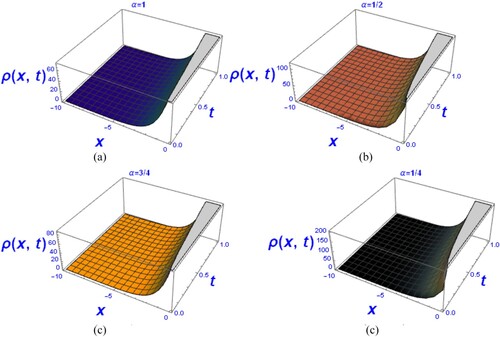
Figure 3. (a–d) Graph of the solution of fractional biological population differential equation for different values of $\alpha$ in Case (i).

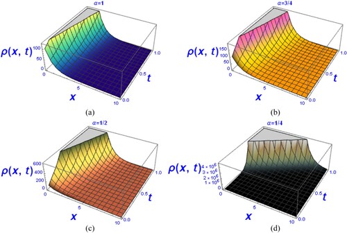
For $0<\alpha \le 1$, these graphs show a rapid increase in population density in an ecosystem that is migrating from an unfavourable zone that never ends, as alpha decreases by solution $\rho \left(x,t\right)=100e^{-x+2t}$ to the classical biological population differential equation in Case (i).

Case (ii): Similarly, we can find the solution of (4.18) and analyse graphically as (4.23) $\rho \left(x,t\right)=P\frac{\cosh mx}{\cosh ma}{E}_{\alpha }\left(\left(m^2+\mu \right)t^{\alpha }\right)$(4.23)

For the sake of convenience, we will set $m=1,a=1,P=100$ and $\mu =1$ to show graphs of the solution (4.23) in Figure 4, without losing generality

Figure 4. (a–d) Graph of the solution of fractional biological population differential equation for different values of $\alpha$ in Case (ii).

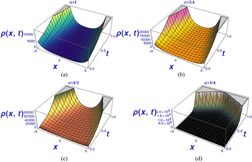
For $0<\alpha \le 1$, as $\alpha$ declines by the solution $\rho \left(x,t\right)=100\frac{\cosh x}{\cosh 1}{e}^{2t}$ to the conventional biological population differential equation in Case (ii), these graphs demonstrate a rapid increase in population density in a suitable habitat around an unfavourable segment on both ends.

Next, we illustrate the special case $0<\alpha \le 1$ for Verhulst law, along with $\text{β}=2$, which is based on probabilistic considerations of walk, in which individuals either stay put or migrate in a population-decreasing direction [33], an unfavourable zone encroaches upon a suitable habitat and extends endlessly in one direction. That is, $-\mathrm{\infty }<x\le a,\rho \left(-\mathrm{\infty },t\right)=0,\rho \left(a,t\right)=P$, $\rho \left(x,0\right)=P{e}^{\frac{1}{2}\sqrt{\lambda }(x-a)}$.

Problem 4.2: We reach at the following fractional biological population equation (4.24) ${}_C{D}_t^{\alpha }\rho \left(x,t\right)=D_x^2{\rho }^2\left(x,t\right)+\mu \rho \left(x,t\right)-\lambda {\rho }^2\left(x,t\right),t\ge 0,x\in \text{R,}$(4.24) with initial conditions $-\mathrm{\infty }<x\le a,\rho \left(-\mathrm{\infty },0\right)=0,\rho \left(a,0\right)=P$, $\rho \left(x,0\right)=P{e}^{\frac{1}{2}\sqrt{\lambda }(x-a)}$.

Solution: In view of (3.6) and (3.7), here we have (4.25) ${\rho }_0\left(x,t\right)=P{e}^{\frac{1}{2}\sqrt{\lambda }(x-a)}\text{and}{\rho }_{k+1}\left(x,t\right)=E^{-1}\left[v^{\alpha }E\left[A_k\left(\rho \left(x,t\right)\right);v\right];t\right].$(4.25) which in view of (4.13), (4.14) and (4.15) gives us $\begin{array}{l}{A}_0=\mu P{e}^{\frac{1}{2}\sqrt{\lambda }(x-a)},{\rho }_1\left(x,t\right)=\mu P{e}^{\frac{1}{2}\sqrt{\lambda }(x-a)}\frac{t^{\alpha }}{\mathrm{\Gamma }\left(\alpha +1\right)},\\ A_1={\mu }^{2}P{e}^{\frac{1}{2}\sqrt{\lambda }(x-a)}\frac{t^{\alpha }}{\mathrm{\Gamma }\left(\alpha +1\right)},{\rho }_2\left(x,t\right)={\mu }^{2}P{e}^{\frac{1}{2}\sqrt{\lambda }(x-a)}\frac{t^{2\alpha }}{\mathrm{\Gamma }\left(2\alpha +1\right)}\\ A_2={\mu }^{3}P{e}^{\frac{1}{2}\sqrt{\lambda }(x-a)}\frac{t^{2\alpha }}{\mathrm{\Gamma }\left(2\alpha +1\right)},{\rho }_3\left(x,t\right)={\mu }^{3}P{e}^{\frac{1}{2}\sqrt{\lambda }(x-a)}\frac{t^{3\alpha }}{\mathrm{\Gamma }\left(3\alpha +1\right)},\\ \end{array}$ and so on.

Resulting in the solution of (4.24) with given initial condition as (4.26) $\rho \left(x,t\right)=P{e}^{\frac{1}{2}\sqrt{\lambda }(x-a)}{E}_{\alpha }\left(\mu t^{\alpha }\right).$(4.26) For the sake of convenience, we will set $\lambda =4,a=0,P=100$ and $\mu =1$ to show graphs of the solution (4.23) in Figure 5, without losing generality

Figure 5. (a–d) Graph of the solution of fractional biological population differential equation for Verhulst law for different values of $\alpha$.

The population density has increased, as seen in these graphs. Individuals that migrate to or remain in an undesirable area that never ends in one direction encroach on a suitable habitat as $\alpha$ lowers by the solution $\rho \left(x,t\right)=100e^{x+t}$ to the classical biological population differential equation for Verhulst law.

5. Conclusion

We have obtained the analytic solutions for fractional relaxation oscillation, fractional damped oscillation and time-fractional biological population differential equations, using the Elzaki decomposition method (EDM). The effectiveness of the method is demonstrated by the predicted accurate analytical solutions and visual observations obtained by varying the order of the fractional derivative to produce various outcomes. The fractional relaxation equation solution $E_{\alpha }\left(-t^{\alpha }\right)$ decays substantially slower than the classical relaxation equation solution. The fractional solution $\begin{array}{l}{E}_{\alpha }\left[-t^{\alpha }\right]+t{E}_{\alpha ,2}\left[-t^{\alpha }\right]\end{array}$ for damped oscillation fractional differential equation only exhibits a few reduced oscillations as a temporary condition, with their number and initial amplitude increasing with $\alpha$. In the time-fractional biological population equation, the population supply$\sigma$ has been considered according to Malthusian law and Verhulst law. Two cases have been studied for Malthusian law, in which an unfavourable zone that extends endlessly in one direction and unfavourable territory is encircled on both ends by a suitable habitat. In all the cases, for $0<\alpha \le 1$, the graphs indicate a sharp rise in population density $\rho$ as $\alpha$ falls and people shift from unfavourable areas towards a good environment.

Acknowledgements

The authors acknowledge the anonymous reviewers for their purported insights, their comments and suggestions for enhancing an earlier draft of the manuscript, as well as for helping to shape the paper as it is now.

Disclosure statement

No potential conflict of interest was reported by the author(s).

Data availability statement

No data were used for this study.

References

- Etemad S, Avci I, Kumar P, et al. Some novel mathematical analysis on the fractal–fractional model of the AH1N1/09 virus and its generalized Caputo-type version. Chaos, Solitons Fractals. 2022;162:112511.
- Butt AI, Ahmad W, Rafiq M, et al. Numerical analysis of Atangana-Baleanu fractional model to understand the propagation of a novel corona virus pandemic. Alexandria Eng J. 2022;61(9):7007–7027.
- Elzaki TM. The new integral transform Elzaki transform. Global J Pure Appl Math. 2011;7(1):57–64.
- Elzaki TM. Application of new transform ‘Elzaki transform’ to partial differential equations. Glob J Pure Appl Math. 2011;7(1):65–70.
- Neamaty A, Agheli B, Darzi R. New integral transform for solving nonlinear partial Differential equations of fractional order. Theory Approx Appl. 2013;10(1):69–86.
- Elzaki TM, Biazar J. Homotopy perturbation method and Elzaki transform for solving system of nonlinear partial differential equations. World Appl Sci J. 2013;24(7):944–948.
- Suleman M, Lu D, Rahman JU, et al. Analytical solution of linear fractionally damped oscillator by Elzaki transformed method. DJ J Eng Appl Math. 2018;4(2):49–57.
- Elzaki TM, Kim H. The solution of radial diffusivity and shock wave equations by Elzaki variational iteration method. Int J Math Anal. 2015;9:1065–1071.
- Rahman J, Lu D, Suleman M, et al. He–Elzaki method for spatial diffusion of biological population. Fractals. 2019 Aug 13;27(05):1950069.
- Khalid M, Sultana M, Zaidi F, et al. An Elzaki transform decomposition algorithm applied to a class of non-linear differential equations. Natural Sci. Res. 2015;5:48–56.
- Achar BN, Hanneken JW, Clarke T. Damping characteristics of a fractional oscillator. Physica A. 2004;339(3-4):311–319.
- Rossikhin YA, Shitikova MV. Application of fractional calculus for dynamic problems of solid mechanics: novel trends and recent results. Appl Mech Rev. 2010;63(1):010801.
- Gorenflo R, Mainardi F. Fractional relaxation-oscillation phenomena. In Handbook of fractional calculus and applications. 2019. p. 45–74.
- Mittag-Leffler GM. Sur la nouvelle fonction. CR Acad Sci Paris. 1903;137(2):554–558.
- Wiman A. Über den Fundamentalsatz in der Teorie der Funktionen Ea (x). Acta Mathematica. 1905;29:191–201.
- Achar BN, Hanneken JW, Enck T, et al. Dynamics of the fractional oscillator. Physica A. 2001;297(3-4):361–367.
- Dayan F, Rafiq M, Ahmed N, et al. Design and numerical analysis of fuzzy nonstandard computational methods for the solution of rumor based fuzzy epidemic model. Physica A. 2022;127542.
- Raza A, Baleanu D, Yousaf M, et al. Modeling of anthrax disease via efficient computing techniques. Intell. Autom. Soft Comput. 2022;32(2):1109–1124.
- Naveed M, Baleanu D, Raza A, et al. Treatment of polio delayed epidemic model via computer simulations. CMC-Comput Mater Continua. 2022;70(2):3415–3431.
- Skellam JG. Random dispersal in theoretical populations. Biometrika. 1951;38(1/2):196–218.
- Gurtin ME, MacCamy RC. On the diffusion of biological populations. Math Biosci. 1977;33(1-2):35–49.
- Okubo A. Diffusion and ecological problems: mathematica1 models; 1980.
- Pielou EC. An introduction to mathematical ecology. New York: Wiley-Inter-science; 1969.
- Morrill R, Gaile GL, Thrall GI. Spatial diffusion; 2020.
- Kheirkhah F, Hajipour M, Baleanu D. The performance of a numerical scheme on the variable-order time-fractional advection-reaction-subdiffusion equations. Appl Numer Math. 2022;178:25–40.
- Upadhyay RK, Iyengar SR. Spatial dynamics and pattern formation in biological populations. New York: Chapman and Hall/CRC; 2021.
- Namazi H, Kulish VV. Fractional diffusion based modelling and prediction of human brain response to external stimuli. Comput Math Methods Med. 2015;2015:1–11.
- Bueno-Orovio A, Kay D, Grau V, et al. Fractional diffusion models of cardiac electrical propagation: role of structural heterogeneity in dispersion of repolarization. J R Soc Interface. 2014;11(97):20140352.
- Maldon B, Thamwattana N. A fractional diffusion model for dye-sensitized solar cells. Molecules. 2020;25(13):2966.
- Ali I, Malik N, Chanane B. Fractional diffusion model for transport through porous media; 2014.
- Jiménez S, Usero D, Vázquez L, et al. Fractional diffusion models for the atmosphere of Mars. Fractal Fract. 2017;2(1):1.
- Purohit SD, Khan AM, Suthar DL, et al. The impact on raise of environmental pollution and occurrence in biological populations pertaining to incomplete H-function. Natl Acad Sci Lett. 2021;44:263–266. DOI:10.1007/s40009-020-00996-y
- Gurney WS, Nisbet RM. The regulation of inhomogeneous populations. J Theor Biol. 1975;52(2):441–457.