A reliable multi-resolution collocation algorithm for nonlinear Schrödinger equation with wave operator

Abstract

The solution of a nonlinear hyperbolic Schrödinger equation (NHSE) is proposed in this paper using the Haar wavelet collocation technique (HWCM). The central difference technique is applied to handle the temporal derivative in the NHSE and the finite Haar functions are introduced to approximate the space derivatives. After linearizing the NHSE, it is transformed into full algebraic form with the help of finite difference and Haar wavelets approximation. Solving this well-conditional system of the algebraic equation, we obtained the required solution. Theoretical convergence and stability analysis of HWCM is also performed for two-dimensional NHSE which is supported by the experimental rate of convergence. The numerical findings for the moving soliton wave in the form of $|\phi |$ are explored in depth using Haar wavelets. The propagation of soliton waves is captured accordingly and the time blow-up phenomenon has also been handled by the proposed HWCM because of the well-conditional behaviour of the transformed algebraic equations. Several examples are presented to demonstrate the proposed method and the results are found correct and efficient. In the last example, we have considered a practical case that has no exact solution.

Keywords:

• Haar functions
• nonlinear hyperbolic Schrödinger equation
• wavelet collocation technique
• linearization
• propagation of soliton wave

Mathematics Subject Classifications:

• 35–02
• 35A25
• 35L20
• 35L70
• 65M22

1. Introduction

The nonlinear hyparabolic Schrödinger equation (NHSE), which is derived from quantum mechanics, is one of the significant models in applied and mathematical physics. This equation is also known as Schrödinger equation with wave operator. It represents an individual reinforcing packet of wave that sustains its structure while it proceeds at a uniform velocity in physics and applied mathematics. The NHSEs have been frequently utilized to simulate a wide range of nonlinear physical processes. Some of the featured applications of NHSEs are related to fiber optic system [1], underwater acoustics [2], quantum physics [3] and shocks phenomena [4]. These books [1–4] are also important from engineering aspect to understanding the behaviour of Schrödinger equations. This equation is also called as Gross–Pitaevskii equation and has an important contribution in the representation of hydrodynamics related to Bose–Einstein condensate [5, 6]. Some other applications of nonlinear phenomena in applied sciences are represented by the system of PDEs [7, 8].

The nonlinear Schrödinger equation attracts the attentions of researchers due to its different types/structures along with important applications in applied sciences. The cubic Schrödinger equations [9] and Schrödinger equations with wave operator [10] are the well-known nonlinear time-dependent partial differential equations (PDEs). These equations also represent different structures of solitons like single soliton, double soliton, bright and dark solitons, vector and dissipative solitons, breathers and dispersion-managed solitons and multiple moving solitons and their collisions.

The solution of NHSE defends a wide field containing nonlinear phenomena in applied sciences like plasma physics, dynamics, nonlinear fiber optics, atmospheric and nuclear systems, molecular biology, nonlinear optics, elastic media and quantum mechanics. The NHSE is defined as follows. Let $u(t,\mathit{x})$ represent a complex-valued function, where $t\in [0,T]$ and $\mathit{x}\in D\subset {\mathbb{R}}^d$, d = 1, or 2. Then the equation has the following non-dimensionalized form (1) $\begin{array}{rl}& \frac{{\mathrm{\partial }}^2\phi (t,\mathit{x})}{\mathrm{\partial }{t}^2}-\mathrm{\Delta }\phi (t,\mathit{x})+i\alpha \frac{\mathrm{\partial }\phi (t,\mathit{x})}{\mathrm{\partial }t}\\ & +(g\left(\mathit{x}\right)+\text{β}\left(\mathit{x}\right)|\phi (t,\mathit{x}){|}^2)\phi (t,\mathit{x})=0,(t,\mathit{x})\in (0,T)\times D,\end{array}$(1) where Δ is the Laplacian operator, $g\left(\mathit{x}\right)$, $\text{β}\left(\mathit{x}\right)$ are functions having real values and $i=\sqrt{-1}$ indicates the imaginary part. Along with (1(1) $\begin{array}{rl}& \frac{{\mathrm{\partial }}^2\phi (t,\mathit{x})}{\mathrm{\partial }{t}^2}-\mathrm{\Delta }\phi (t,\mathit{x})+i\alpha \frac{\mathrm{\partial }\phi (t,\mathit{x})}{\mathrm{\partial }t}\\ & +(g\left(\mathit{x}\right)+\text{β}\left(\mathit{x}\right)|\phi (t,\mathit{x}){|}^2)\phi (t,\mathit{x})=0,(t,\mathit{x})\in (0,T)\times D,\end{array}$(1) ), the following given information are called the initial and boundary conditions, respectively (2) $\phi (0,\mathit{x})=u_0\left(\mathit{x}\right),\frac{\mathrm{\partial }\phi (0,\mathit{x})}{\mathrm{\partial }t}={\dot{u}}_0\left(\mathit{x}\right),\mathit{x}\in D,$(2) and, for $0\le t\le T$, (3) $\begin{array}{rl}& \phi (t,a)={\psi }_0\left(t\right),\phi (t,b)={\psi }_1\left(t\right),\mathrm{f}\mathrm{o}\mathrm{r}d=1,\end{array}$(3) (4) $\begin{array}{rl}& \{\begin{array}{l}\phi (t,a,y)={\psi }_0(y,t),\phi (t,b,y)={\psi }_1(y,t),y\in [a,b],\\ \phi (t,x,a)={\phi }_0(x,t),\phi (t,x,b)={\phi }_1(x,t),x\in [a,b],\end{array}\mathrm{f}\mathrm{o}\mathrm{r}d=2.\end{array}$(4) Due to the nonlinear behaviour of the NHSE, it is usually complicated and sometimes not possible to find its exact solution [9, 11], therefore numerical treatment is an alternative approach to get its solution. The solution or movement of the wave depends on the given information called initial condition to the differential equation. A preference is given to the numerical technique to solve NHSE numerically, due to the unavailability of the exact solution. It is mandatory to mention that the traditional techniques for Schrödinger equation give unstable and inaccurate results and cause numerical blow-up. Some of the techniques which handle this equation with acceptable accuracy are modified finite difference approaches [12–14], spline mesh-based method [15], Galerkin method [16], Multi-symplectic integrator [17] and Fourier pseudospectral techniques [18, 19]. Literature suggests to prefer the conservative schemes to minimize these issues [13, 20, 21] instead of nonconservative scheme [22]. Few related latest contributions are also reported in [23, 24].

The Schrödinger-type equation has such a wide range of applications in various real-world situations, therefore an efficient and accurate numerical solver is the need of the scientist and engineers. Different numerical schemes have been investigated to get acceptable results to the Schrödinger equation, i.e. finite element method [25], Dufort–Frankel scheme [26], time-splitting spectral method [27, 28], inverse scattering transform method [29], multi-quadrics quasi-interpolation scheme [30], finite difference method [31], Jacobi–Gauss–Lobatto method [32], cubic B-spline method [33], Legendre spectral element method [34] and the references therein. Some of the latest contributions for nonlinear Schrödinger equations with different types of solitons are highlighted in [35–43]. Nonlinear Schrödinger equation is also studied in fractional differential equations [44–48] and has very superiorities in the field of applied science nowadays.

In recent decay, the investigation has been concentrated on the wavelet application to the problems related to physics and applied sciences. As an integration tool, wavelets are used to solve differential equations, i.e. wavelet meshless approach [49], Daubechies wavelet method [50], wavelet-based Galerkin approach [51] and wavelet mesh-based methods [52–54]. An intensive presentation of the wavelet-based techniques for the solution of various differential problems is given in [55].

Differential equations like ordinary, partial and integro-differential equations have been used to model complex engineering and physical systems and the Haar wavelets were applied to tackle these types of problems in [56–62]. The stimulating problems related to the fractional operator have associated the further importance of applicability of Haar wavelet techniques [63–67]. In order to detect software piracy, the most sophisticated development by Haar wavelets is conducted in [68]. The Haar wavelets are also used to find the different types of source functions in the linear and nonlinear inverse problems [53, 54, 69–72].

1.1. Schrödinger equations and Haar wavelet-based approach

Haar wavelets are also in practice to solve nonlinear Schrödinger equations. In [73] the nonlinear parabolic Schrödinger equations have been solved by a stable Haar wavelet collocation method (HWCM), where the simple linearization technique has been adopted to handle this problem. In [9], the cubic $(1+2)$ Schrödinger equation has been converted into system of PDEs by using $u(x,t)=r(x,t)+is(x,t)$, which are then solved through HWCM. The two-dimensional nonlinear parabolic Schrödinger equation has been accurately solved by HWCM with stability analysis [74]. In [24] an efficient and conservative method based on Haar function is presented for one-dimensional NHSE, where the central difference scheme is used to approximate the time derivatives and the space derivatives are approximated by finite Haar functions. The one-dimensional NHSE is then transform it to full algebraic form with the help Haar function approximation.

1.2. The main purpose of this work

In main objective of this article is to present an efficient and accurate method based on Haar function for two-dimensional NHSE having constant and variable coefficients. Based on this approach, the central difference scheme is used to approximate the time derivatives and the space derivatives are approximated by finite Haar functions. The two-dimensional NHSE can be transformed in to full algebraic form with the help Haar function approximation after linearizing the NHSE. Instead of simple linearization technique, we linearized the nonlinear term by taking the average of results obtained in previous and next time steps i.e. $|u(t,\mathit{x}){|}^{2}u(t,\mathit{x})=|u(t_o,\mathit{x}){|}^2\left(u\right(t_o,\mathit{x})+u(t,\mathit{x}\left)\right)/2$, where $t_o$ and t represent previous and next time levels, respectively. This linearization technique is more suitable for capturing the soliton movements and results are acceptable.

The structure of the paper is as follows: the definition of the Haar function and its antiderivatives are covered in Section 2, which serve as the foundation for an approximate solution. Section 3, introduces the Haar wavelet approximation. The stability and convergence analysis of the HWCM is discussed in Section 4. The computed results are presented in Section 5, and the final remarks are presented in Section 6.

2. Haar functions

A generalized representation of the Haar functions is defined as (5) $h_i\left(x\right)=\{\begin{array}{ll}1& \mathrm{f}\mathrm{o}\mathrm{r}x\in \left[{\zeta }_1\right(i),{\zeta }_2(i\left)\right),\\ -1& \mathrm{f}\mathrm{o}\mathrm{r}x\in \left[{\zeta }_2\right(i),{\zeta }_3(i\left)\right),\\ 0& \mathrm{e}\mathrm{l}\mathrm{s}\mathrm{e}\mathrm{w}\mathrm{h}\mathrm{e}\mathrm{r}\mathrm{e},\end{array}$(5) where (6) $\{\begin{array}{rl}& {\zeta }_1\left(i\right)=a+\frac{(b-a)}{m}k,{\zeta }_2\left(i\right)=a+\frac{(b-a)}{m}(k+0.5),\\ & {\zeta }_3\left(i\right)=a+\frac{(b-a)}{m}(k+1),\\ & i=m+k+1,k=0,1,\dots ,m-1,m=2^j,j=0,1,\dots .\end{array}$(6) Here the wavelet's distinct levels are determined by m, while k determined the translation parameter. We note that $i\ge 2$. We define $h_1\left(x\right)=\{\begin{array}{ll}1& \mathrm{f}\mathrm{o}\mathrm{r}x\in [a,b],\\ 0& \mathrm{e}\mathrm{l}\mathrm{s}\mathrm{e}\mathrm{w}\mathrm{h}\mathrm{e}\mathrm{r}\mathrm{e}.\end{array}$We called $h_1\left(x\right)$ the mother wavelet. We will use certain notations for the following integrals to make the derivations easier for $i=2,3,4,\dots$ $\begin{array}{rl}{p}_{i,1}\left(x\right)& ={\int }_a^x{h}_i\left(x^{\prime }\right)\mathrm{d}{x}^{\prime }\\ & =\{\begin{array}{ll}0& \mathrm{f}\mathrm{o}\mathrm{r}x<{\zeta }_1\left(i\right),\\ x-{\zeta }_1\left(i\right)& \mathrm{f}\mathrm{o}\mathrm{r}x\in \left[{\zeta }_1\right(i),{\zeta }_2(i\left)\right),\\ x-{\zeta }_1\left(i\right)-2(x-{\zeta }_2(i\left)\right)& \mathrm{f}\mathrm{o}\mathrm{r}x\in \left[{\zeta }_2\right(i),{\zeta }_3(i\left)\right),\\ x-{\zeta }_1\left(i\right)-2(x-{\zeta }_2(i\left)\right)+(x-{\zeta }_3(i\left)\right)& \mathrm{f}\mathrm{o}\mathrm{r}x\ge {\zeta }_3\left(i\right),\end{array}\\ p_{i,2}\left(x\right)& ={\int }_a^x{p}_{i,1}\left(x^{\prime }\right)\mathrm{d}{x}^{\prime }\\ & =\{\begin{array}{ll}0& \mathrm{f}\mathrm{o}\mathrm{r}x<{\zeta }_1\left(i\right),\\ {\displaystyle \frac{1}{2}}(x-{\zeta }_1(i){)}^2& \mathrm{f}\mathrm{o}\mathrm{r}x\in \left[{\zeta }_1\right(i),{\zeta }_2(i\left)\right),\\ {\displaystyle \frac{1}{2}}\left[\right(x-{\zeta }_1\left(i\right){)}^2-2(x-{\zeta }_2(i\left){)}^2\right]& \mathrm{f}\mathrm{o}\mathrm{r}x\in \left[{\zeta }_2\right(i),{\zeta }_3(i\left)\right),\\ {\displaystyle \frac{1}{2}}\left[\right(x-{\zeta }_1\left(i\right){)}^2-2(x-{\zeta }_2(i){)}^2+(x-{\zeta }_3\left(i\right){)}^2]& \mathrm{f}\mathrm{o}\mathrm{r}x\ge {\zeta }_3\left(i\right),\end{array}\end{array}$and (7) $C_i={\int }_a^b{p}_{i,1}\left(x^{\prime }\right)\mathrm{d}{x}^{\prime }=\frac{(b-a{)}^2}{4m^2}.$(7) For i = 1 the integrals of the Haar functions are [58] $p_{1,1}\left(x\right)=x-a\mathrm{a}\mathrm{n}\mathrm{d}{p}_{1,2}\left(x\right)=\frac{(x-a{)}^2}{2}.$It's important to note that the formula below has been established in [75] (8) $\underset{a\le s\le b}{max}\left(p_{i,2}\right(x\left)\right)=\frac{(b-a{)}^2}{4m^2}.$(8)

3. HWCM for two-dimensional NHSE

To solve nonlinear Schrödinger equation (9) $\begin{array}{rl}& \frac{{\mathrm{\partial }}^2\phi (t,x,y)}{\mathrm{\partial }{t}^2}-\frac{{\mathrm{\partial }}^2\phi (t,x,y)}{\mathrm{\partial }{x}^2}-\frac{{\mathrm{\partial }}^2\phi (t,x,y)}{\mathrm{\partial }{y}^2}+i\alpha \frac{\mathrm{\partial }\phi (t,x,y)}{\mathrm{\partial }t}\\ & +(g(x,y)+\text{β}(x,y)|\phi (t,x,y){|}^2)\phi (t,x,y)=0,\end{array}$(9) along with the conditions defined in Equations (2(2) $\phi (0,\mathit{x})=u_0\left(\mathit{x}\right),\frac{\mathrm{\partial }\phi (0,\mathit{x})}{\mathrm{\partial }t}={\dot{u}}_0\left(\mathit{x}\right),\mathit{x}\in D,$(2) )–(4(4) $\begin{array}{rl}& \{\begin{array}{l}\phi (t,a,y)={\psi }_0(y,t),\phi (t,b,y)={\psi }_1(y,t),y\in [a,b],\\ \phi (t,x,a)={\phi }_0(x,t),\phi (t,x,b)={\phi }_1(x,t),x\in [a,b],\end{array}\mathrm{f}\mathrm{o}\mathrm{r}d=2.\end{array}$(4) ) with the help of Haar functions, we approximate the highest derivative with the following series (10) $\frac{{\mathrm{\partial }}^2\phi (t,x,y)}{\mathrm{\partial }{x}^2}=\sum _{\ell =1}^{\mathrm{\infty }}\sum _{i=1}^{\mathrm{\infty }}{a}_{i\ell }\left(t\right)h_i\left(x\right)h_{\ell }\left(y\right)$(10) and (11) $\frac{{\mathrm{\partial }}^2\phi (t,x,y)}{\mathrm{\partial }{y}^2}=\sum _{\ell =1}^{\mathrm{\infty }}\sum _{i=1}^{\mathrm{\infty }}{b}_{i\ell }\left(t\right)h_i\left(x\right)h_{\ell }\left(y\right),$(11) where $a_{i\ell }\left(t\right)$ and $b_{i\ell }\left(t\right)$ are the coefficients and can be determined by, see [76], $\begin{array}{rl}{a}_{i\ell }\left(t\right)& ={\int }_a^b{\int }_a^b\frac{{\mathrm{\partial }}^2\phi (t,x,y)}{\mathrm{\partial }{x}^2}{h}_i\left(x\right)h_{\ell }\left(y\right)\mathrm{d}x\mathrm{d}y,\mathrm{a}\mathrm{n}\mathrm{d}\\ b_{i\ell }\left(t\right)& ={\int }_a^b{\int }_a^b\frac{{\mathrm{\partial }}^2\phi (t,x,y)}{\mathrm{\partial }{y}^2}{h}_i\left(x\right)h_{\ell }\left(y\right)\mathrm{d}x\mathrm{d}y.\end{array}$With the help of mean value theorem and noting the definition of $h_i\left(x\right)$ given in Equations (5(5) $h_i\left(x\right)=\{\begin{array}{ll}1& \mathrm{f}\mathrm{o}\mathrm{r}x\in \left[{\zeta }_1\right(i),{\zeta }_2(i\left)\right),\\ -1& \mathrm{f}\mathrm{o}\mathrm{r}x\in \left[{\zeta }_2\right(i),{\zeta }_3(i\left)\right),\\ 0& \mathrm{e}\mathrm{l}\mathrm{s}\mathrm{e}\mathrm{w}\mathrm{h}\mathrm{e}\mathrm{r}\mathrm{e},\end{array}$(5) ) and (6(6) $\{\begin{array}{rl}& {\zeta }_1\left(i\right)=a+\frac{(b-a)}{m}k,{\zeta }_2\left(i\right)=a+\frac{(b-a)}{m}(k+0.5),\\ & {\zeta }_3\left(i\right)=a+\frac{(b-a)}{m}(k+1),\\ & i=m+k+1,k=0,1,\dots ,m-1,m=2^j,j=0,1,\dots .\end{array}$(6) ), we obtain $\begin{array}{rl}{a}_{i\ell }\left(t\right)& ={\int }_a^b({\int }_{{\zeta }_1\left(i\right)}^{{\zeta }_2\left(i\right)}\frac{{\mathrm{\partial }}^2\phi (t,x,y)}{\mathrm{\partial }{x}^2}\mathrm{d}x-{\int }_{{\zeta }_2\left(i\right)}^{{\zeta }_3\left(i\right)}\frac{{\mathrm{\partial }}^2\phi (t,x,y)}{\mathrm{\partial }{x}^2}\mathrm{d}x)h_{\ell }\left(y\right)\mathrm{d}y\\ & ={\int }_a^b\left(({\zeta }_2\right(i)-{\zeta }_1(i))\frac{{\mathrm{\partial }}^2\phi ({\xi }_1,y,t)}{\mathrm{\partial }{x}^2}-({\zeta }_3(i)-{\zeta }_2(i\left))\frac{{\mathrm{\partial }}^2\phi ({\xi }_2,y,t)}{\mathrm{\partial }{x}^2}\right)h_{\ell }\left(y\right)\mathrm{d}y\\ & =\frac{b-a}{2^{j+1}}{\int }_a^b(\frac{{\mathrm{\partial }}^2\phi ({\xi }_1,y,t)}{\mathrm{\partial }{x}^2}-\frac{{\mathrm{\partial }}^2\phi ({\xi }_2,y,t)}{\mathrm{\partial }{x}^2})h_{\ell }\left(y\right)\mathrm{d}y\\ & =\frac{b-a}{2^{j+1}}{\int }_a^b({\xi }_1-{\xi }_2)\frac{{\mathrm{\partial }}^3\phi ({\xi }_3,y,t)}{\mathrm{\partial }{x}^3}{h}_{\ell }\left(y\right)\mathrm{d}y\\ & =\frac{b-a}{2^{j+1}}\left({\int }_{{\zeta }_1\left(\ell \right)}^{{\zeta }_2\left(\ell \right)}\right({\xi }_1-{\xi }_2)\frac{{\mathrm{\partial }}^3\phi ({\xi }_3,y,t)}{\mathrm{\partial }{x}^3}\mathrm{d}y-{\int }_{{\zeta }_2\left(\ell \right)}^{{\zeta }_3\left(\ell \right)}({\xi }_1-{\xi }_2\left)\frac{{\mathrm{\partial }}^3\phi ({\xi }_3,y,t)}{\mathrm{\partial }{x}^3}\mathrm{d}y\right)\end{array}$for any constant ${\xi }_1\in \left({\zeta }_1\right(i),{\zeta }_2(i\left)\right)$, ${\xi }_2\in \left({\zeta }_2\right(i),{\zeta }_3(i\left)\right)$, and ${\xi }_3\in ({\xi }_1,{\xi }_2)$. Again applying the mean value theorem with the fact that $|{\xi }_1-{\xi }_2|\le |{\zeta }_3\left(i\right)-{\zeta }_1\left(i\right)|\le \frac{1}{2^j},$we obtain (12) $|a_{i\ell }\left(t\right)|\le \frac{c}{2^{4j}}\underset{a\le x,y\le b}{max}\left|\frac{{\mathrm{\partial }}^4\phi (t,x,y)}{\mathrm{\partial }y\mathrm{\partial }{x}^3}\right|$(12) for some positive constant c. In the same way (13) $|b_{i\ell }\left(t\right)|\le \frac{c}{2^{4j}}\underset{a\le x,y\le b}{max}\left|\frac{{\mathrm{\partial }}^4\phi (t,x,y)}{\mathrm{\partial }x\mathrm{\partial }{y}^3}\right|.$(13) Applying the definite integration from a to x on Equation (10(10) $\frac{{\mathrm{\partial }}^2\phi (t,x,y)}{\mathrm{\partial }{x}^2}=\sum _{\ell =1}^{\mathrm{\infty }}\sum _{i=1}^{\mathrm{\infty }}{a}_{i\ell }\left(t\right)h_i\left(x\right)h_{\ell }\left(y\right)$(10) ) w.r.t. x and noting Equation (7(7) $C_i={\int }_a^b{p}_{i,1}\left(x^{\prime }\right)\mathrm{d}{x}^{\prime }=\frac{(b-a{)}^2}{4m^2}.$(7) ), we acquire (14) $\frac{\mathrm{\partial }\phi (t,x,y)}{\mathrm{\partial }x}=\frac{\mathrm{\partial }\phi (a,y,t)}{\mathrm{\partial }x}+\sum _{\ell =1}^{\mathrm{\infty }}\sum _{i=1}^{\mathrm{\infty }}{a}_{i\ell }\left(t\right)p_{i,1}\left(x\right)h_{\ell }\left(y\right).$(14) Now again taking definite integration from a to b of Equation (14(14) $\frac{\mathrm{\partial }\phi (t,x,y)}{\mathrm{\partial }x}=\frac{\mathrm{\partial }\phi (a,y,t)}{\mathrm{\partial }x}+\sum _{\ell =1}^{\mathrm{\infty }}\sum _{i=1}^{\mathrm{\infty }}{a}_{i\ell }\left(t\right)p_{i,1}\left(x\right)h_{\ell }\left(y\right).$(14) ) w.r.t. x and by simplifying furthermore (15) $\frac{\mathrm{\partial }\phi (a,y,t)}{\mathrm{\partial }x}=\frac{\phi (b,y,t)-\phi (a,y,t)}{(b-a)}-\sum _{\ell =1}^{\mathrm{\infty }}\sum _{i=1}^{\mathrm{\infty }}{a}_{i\ell }\left(t\right)\frac{C_i}{(b-a)}{h}_{\ell }\left(y\right).$(15) Inserting Equation (15(15) $\frac{\mathrm{\partial }\phi (a,y,t)}{\mathrm{\partial }x}=\frac{\phi (b,y,t)-\phi (a,y,t)}{(b-a)}-\sum _{\ell =1}^{\mathrm{\infty }}\sum _{i=1}^{\mathrm{\infty }}{a}_{i\ell }\left(t\right)\frac{C_i}{(b-a)}{h}_{\ell }\left(y\right).$(15) ) into Equation (14(14) $\frac{\mathrm{\partial }\phi (t,x,y)}{\mathrm{\partial }x}=\frac{\mathrm{\partial }\phi (a,y,t)}{\mathrm{\partial }x}+\sum _{\ell =1}^{\mathrm{\infty }}\sum _{i=1}^{\mathrm{\infty }}{a}_{i\ell }\left(t\right)p_{i,1}\left(x\right)h_{\ell }\left(y\right).$(14) ) and then taking definite integration from a to x, we acquire (16) $\phi (t,x,y)={\tilde{\phi }}_o(t,x,y)+\sum _{\ell =1}^{\mathrm{\infty }}\sum _{i=1}^{\mathrm{\infty }}{a}_{i\ell }\left(t\right){\tilde{h}}_i\left(x\right)h_{\ell }\left(y\right),$(16) where ${\tilde{\phi }}_o(t,x,y)=\phi (a,y,t)+(x-a){\overline{\phi }}_o(y,t)$, ${\overline{\phi }}_o(y,t)=\left(\phi \right(b,y,t)-\phi (a,y,t\left)\right)/(b-a)$ and (17) ${\tilde{h}}_i\left(x\right)=p_{i,2}\left(x\right)-(x-a)\frac{C_i}{b-a}.$(17) Similarly, following the steps from Equations (14(14) $\frac{\mathrm{\partial }\phi (t,x,y)}{\mathrm{\partial }x}=\frac{\mathrm{\partial }\phi (a,y,t)}{\mathrm{\partial }x}+\sum _{\ell =1}^{\mathrm{\infty }}\sum _{i=1}^{\mathrm{\infty }}{a}_{i\ell }\left(t\right)p_{i,1}\left(x\right)h_{\ell }\left(y\right).$(14) )–(16(16) $\phi (t,x,y)={\tilde{\phi }}_o(t,x,y)+\sum _{\ell =1}^{\mathrm{\infty }}\sum _{i=1}^{\mathrm{\infty }}{a}_{i\ell }\left(t\right){\tilde{h}}_i\left(x\right)h_{\ell }\left(y\right),$(16) ) and at this time applying integration w.r.t. y to Equation (11(11) $\frac{{\mathrm{\partial }}^2\phi (t,x,y)}{\mathrm{\partial }{y}^2}=\sum _{\ell =1}^{\mathrm{\infty }}\sum _{i=1}^{\mathrm{\infty }}{b}_{i\ell }\left(t\right)h_i\left(x\right)h_{\ell }\left(y\right),$(11) ), we obtain (18) $\frac{\mathrm{\partial }\phi (t,x,y)}{\mathrm{\partial }y}={\overline{\phi }}_l(x,t)+\sum _{\ell =1}^{\mathrm{\infty }}\sum _{i=1}^{\mathrm{\infty }}{b}_{i\ell }\left(t\right)h_i\left(x\right){\overline{h}}_{\ell }\left(y\right),$(18) and $\phi (t,x,y)={\tilde{\phi }}_l(t,x,y)+\sum _{\ell =1}^{\mathrm{\infty }}\sum _{i=1}^{\mathrm{\infty }}{b}_{i\ell }\left(t\right)h_i\left(x\right){\tilde{h}}_{\ell }\left(y\right),$where ${\tilde{\phi }}_l(t,x,y)=\phi (x,a,t)+(y-a){\overline{\phi }}_l(x,t)$ and ${\overline{\phi }}_l(x,t)=\left(\phi \right(x,b,t)-\phi (x,a,t\left)\right)/(b-a)$.

The Equation (9(9) $\begin{array}{rl}& \frac{{\mathrm{\partial }}^2\phi (t,x,y)}{\mathrm{\partial }{t}^2}-\frac{{\mathrm{\partial }}^2\phi (t,x,y)}{\mathrm{\partial }{x}^2}-\frac{{\mathrm{\partial }}^2\phi (t,x,y)}{\mathrm{\partial }{y}^2}+i\alpha \frac{\mathrm{\partial }\phi (t,x,y)}{\mathrm{\partial }t}\\ & +(g(x,y)+\text{β}(x,y)|\phi (t,x,y){|}^2)\phi (t,x,y)=0,\end{array}$(9) ) can be linearized in the following way, where $t_n$ and $t_{n+1}$ are the current and next time levels accordingly (19) $\begin{array}{rl}& \frac{{\mathrm{\partial }}^2\phi (t_{n+1},x,y)}{\mathrm{\partial }{t}^2}-\frac{{\mathrm{\partial }}^2\phi (t_{n+1},x,y)}{\mathrm{\partial }{x}^2}-\frac{{\mathrm{\partial }}^2\phi (t_{n+1},x,y)}{\mathrm{\partial }{y}^2}+i\alpha \frac{\mathrm{\partial }\phi (t_{n+1},x,y)}{\mathrm{\partial }t}\\ & +(g(x,y)+\text{β}(x,y)|\phi (t_n,x,y){|}^2)\left(\frac{\phi (t_{n+1},x,y)+\phi (t_n,x,y)}{2}\right)=0.\end{array}$(19) Using central difference approximation for the time derivatives, we get (20) $\begin{array}{rl}& \frac{\phi (t_{n+1},x,y)-2\phi (t_n,x,y)+\phi (t_{n-1},x,y)}{\mathrm{\Delta }{t}^2}+\mathcal{O}\left(\mathrm{\Delta }{t}^2\right)-\frac{{\mathrm{\partial }}^2\phi (t_{n+1},x,y)}{\mathrm{\partial }{x}^2}-\frac{{\mathrm{\partial }}^2\phi (t_{n+1},x,y)}{\mathrm{\partial }{y}^2}\\ & +i\alpha \frac{\phi (t_{n+1},x,y)-\phi (t_{n-1},x,y)}{2\mathrm{\Delta }t}\\ & +(g(x,y)+\text{β}(x,y)|\phi (t_n,x,y){|}^2)\left(\frac{\phi (t_{n+1},x,y)+\phi (t_n,x,y)}{2}\right)=0.\end{array}$(20) We fixed wavelet resolution J for our computation such that $M=2^J$ and define (21) ${\phi }_M(t,x,y)={\tilde{\phi }}_o(t,x,y)+\sum _{\ell =1}^{2M}\sum _{i=1}^{2M}{a}_{i\ell }\left(t\right){\tilde{h}}_i\left(x\right)h_{\ell }\left(y\right),$(21) ord (22) ${\phi }_M(t,x,y)={\tilde{\phi }}_l(t,x,y)+\sum _{\ell =1}^{2M}\sum _{i=1}^{2M}{b}_{i\ell }\left(t\right)h_i\left(x\right){\tilde{h}}_{\ell }\left(y\right).$(22) Taking two times derivative of Equation (21(21) ${\phi }_M(t,x,y)={\tilde{\phi }}_o(t,x,y)+\sum _{\ell =1}^{2M}\sum _{i=1}^{2M}{a}_{i\ell }\left(t\right){\tilde{h}}_i\left(x\right)h_{\ell }\left(y\right),$(21) ) w.r.t x, we acquire $\begin{array}{rl}\frac{\mathrm{\partial }{\phi }_M(t,x,y)}{\mathrm{\partial }x}& ={\overline{\phi }}_o(y,t)+\sum _{\ell =1}^{2M}\sum _{i=1}^{2M}{a}_{i\ell }\left(t\right){\overline{h}}_i\left(x\right)h_{\ell }\left(y\right),\\ \frac{{\mathrm{\partial }}^2{\phi }_M(t,x,y)}{\mathrm{\partial }{x}^2}& =\sum _{\ell =1}^{2M}\sum _{i=1}^{2M}{a}_{i\ell }\left(t\right)h_i\left(x\right)h_{\ell }\left(y\right).\end{array}$Similarly, from Equation (22(22) ${\phi }_M(t,x,y)={\tilde{\phi }}_l(t,x,y)+\sum _{\ell =1}^{2M}\sum _{i=1}^{2M}{b}_{i\ell }\left(t\right)h_i\left(x\right){\tilde{h}}_{\ell }\left(y\right).$(22) ), we also obtain $\begin{array}{rl}\frac{\mathrm{\partial }{\phi }_M(t,x,y)}{\mathrm{\partial }y}& ={\overline{\phi }}_l(x,t)+\sum _{\ell =1}^{2M}\sum _{i=1}^{2M}{b}_{i\ell }\left(t\right)h_i\left(x\right){\overline{h}}_{\ell }\left(y\right),\\ \frac{{\mathrm{\partial }}^2{\phi }_M(t,x,y)}{\mathrm{\partial }{y}^2}& =\sum _{\ell =1}^{2M}\sum _{i=1}^{2M}{b}_{i\ell }\left(t\right)h_i\left(x\right)h_{\ell }\left(y\right).\end{array}$There is a relationship between Haar approximate and Haar exact expressions like $\begin{array}{rl}{\phi }_M(t,x,y)& =\phi (t,x,y)-E_H^M(t,x,y),\\ \frac{\mathrm{\partial }{\phi }_M(t,x,y)}{\mathrm{\partial }x}& =\frac{\mathrm{\partial }\phi (t,x,y)}{\mathrm{\partial }x}-\frac{\mathrm{\partial }{E}_H^M(t,x,y)}{\mathrm{\partial }x},\\ \frac{{\mathrm{\partial }}^2{\phi }_M(t,x,y)}{\mathrm{\partial }{x}^2}& =\frac{{\mathrm{\partial }}^2\phi (t,x,y)}{\mathrm{\partial }{x}^2}-\frac{{\mathrm{\partial }}^2{E}_H^M(t,x,y)}{\mathrm{\partial }{x}^2},\\ \frac{\mathrm{\partial }{\phi }_M(t,x,y)}{\mathrm{\partial }y}& =\frac{\mathrm{\partial }\phi (t,x,y)}{\mathrm{\partial }y}-\frac{\mathrm{\partial }{E}_H^M(t,x,y)}{\mathrm{\partial }y},\\ \frac{{\mathrm{\partial }}^2{\phi }_M(t,x,y)}{\mathrm{\partial }{y}^2}& =\frac{{\mathrm{\partial }}^2\phi (t,x,y)}{\mathrm{\partial }{y}^2}-\frac{{\mathrm{\partial }}^2{E}_H^M(t,x,y)}{\mathrm{\partial }{y}^2},\end{array}$

where $E_H^M(t,x,y)=\sum _{j=2M+1}^{\mathrm{\infty }}\sum _{i=2M+1}^{\mathrm{\infty }}{a}_{i\ell }\left(t\right){\tilde{h}}_i\left(x\right)h_{\ell }\left(y\right)$or $E_H^M(t,x,y)=\sum _{j=2M+1}^{\mathrm{\infty }}\sum _{i=2M+1}^{\mathrm{\infty }}{b}_{i\ell }\left(t\right)h_i\left(x\right){\tilde{h}}_{\ell }\left(y\right),$and $\begin{array}{rl}\frac{\mathrm{\partial }{E}_H^M(t,x,y)}{\mathrm{\partial }x}& =\sum _{j=2M+1}^{\mathrm{\infty }}\sum _{i=2M+1}^{\mathrm{\infty }}{a}_{i\ell }\left(t\right){\overline{h}}_i\left(x\right)h_{\ell }\left(y\right),\\ \frac{{\mathrm{\partial }}^2{E}_H^M(t,x,y)}{\mathrm{\partial }{x}^2}& =\sum _{j=2M+1}^{\mathrm{\infty }}\sum _{i=2M+1}^{\mathrm{\infty }}{a}_{i\ell }\left(t\right)h_i\left(x\right)h_{\ell }\left(y\right),\\ \frac{\mathrm{\partial }{E}_H^M(t,x,y)}{\mathrm{\partial }y}& =\sum _{j=2M+1}^{\mathrm{\infty }}\sum _{i=2M+1}^{\mathrm{\infty }}{b}_{i\ell }\left(t\right)h_i\left(x\right){\overline{h}}_{\ell }\left(y\right),\\ \frac{{\mathrm{\partial }}^2{E}_H^M(t,x,y)}{\mathrm{\partial }{y}^2}& =\sum _{j=2M+1}^{\mathrm{\infty }}\sum _{i=2M+1}^{\mathrm{\infty }}{b}_{i\ell }\left(t\right)h_i\left(x\right)h_{\ell }\left(y\right).\end{array}$Hence, the exact representation of Equation (20(20) $\begin{array}{rl}& \frac{\phi (t_{n+1},x,y)-2\phi (t_n,x,y)+\phi (t_{n-1},x,y)}{\mathrm{\Delta }{t}^2}+\mathcal{O}\left(\mathrm{\Delta }{t}^2\right)-\frac{{\mathrm{\partial }}^2\phi (t_{n+1},x,y)}{\mathrm{\partial }{x}^2}-\frac{{\mathrm{\partial }}^2\phi (t_{n+1},x,y)}{\mathrm{\partial }{y}^2}\\ & +i\alpha \frac{\phi (t_{n+1},x,y)-\phi (t_{n-1},x,y)}{2\mathrm{\Delta }t}\\ & +(g(x,y)+\text{β}(x,y)|\phi (t_n,x,y){|}^2)\left(\frac{\phi (t_{n+1},x,y)+\phi (t_n,x,y)}{2}\right)=0.\end{array}$(20) ) using Haar wavelets is $\begin{array}{rl}& \frac{{\phi }_M(t_{n+1},x,y)-2{\phi }_M(t_n,x,y)+{\phi }_M(t_{n-1},x,y)}{\mathrm{\Delta }{t}^2}\\ & +\frac{E_H^M(t_{n+1},x,y)-2E_H^M(t_n,x,y)+E_H^M(t_{n-1},x,y)}{\mathrm{\Delta }{t}^2}\\ & -\frac{{\mathrm{\partial }}^2{\phi }_M(t_{n+1},x,y)}{\mathrm{\partial }{x}^2}-\frac{{\mathrm{\partial }}^2{E}_H^M(t_{n+1},x,y)}{\mathrm{\partial }{x}^2}-\frac{{\mathrm{\partial }}^2{\phi }_M(t_{n+1},x,y)}{\mathrm{\partial }{y}^2}-\frac{{\mathrm{\partial }}^2{E}_H^M(t_{n+1},x,y)}{\mathrm{\partial }{y}^2}\\ & +i\alpha \frac{{\phi }_M(t_{n+1},x,y)-{\phi }_M(t_{n-1},x,y)}{2\mathrm{\Delta }t}+i\alpha \frac{E_H^M(t_{n+1},x,y)-E_H^M(t_{n-1},x,y)}{2\mathrm{\Delta }t}\\ & +(g(x,y)+\text{β}(x,y)|{\phi }_M(t_n,x,y){|}^2)\left(\frac{{\phi }_M(t_{n+1},x,y)+{\phi }_M(t_n,x,y)}{2}\right)\\ & +(g(x,y)+\text{β}(x,y)|E_H^M(t_n,x,y){|}^2)\left(\frac{E_H^M(t_{n+1},x,y)+E_H^M(t_n,x,y)}{2}\right)+\mathcal{O}\left(\mathrm{\Delta }{t}^2\right)=0.\end{array}$

Neglecting all the error terms and introducing the nodal points $\begin{array}{r}{x}_l=a+\frac{(b-a)(l-0.5)}{2M}\mathrm{a}\mathrm{n}\mathrm{d}{y}_s=a+\frac{(b-a)(s-0.5)}{2M},\mathrm{f}\mathrm{o}\mathrm{r}l,s=1,2,\dots ,2M,\end{array}$we have formally (23) $\begin{array}{rl}& {\phi }_M(t_{n+1},x_l,y_s)-\mathrm{\Delta }{t}^2\frac{{\mathrm{\partial }}^2{\phi }_M(t_{n+1},x_l,y_s)}{\mathrm{\partial }{x}^2}-\mathrm{\Delta }{t}^2\frac{{\mathrm{\partial }}^2{\phi }_M(t_{n+1},x_l,y_s)}{\mathrm{\partial }{y}^2}+i\frac{\mathrm{\Delta }t}{2}\alpha {\phi }_M(t_{n+1},x_l,y_s)\\ & +\mathrm{\Delta }{t}^2(g(x_l,y_s)+\text{β}(x_l,y_s)|{\phi }_M(t_n,x_l,y_s){|}^2)\left(\frac{{\phi }_M(t_{n+1},x_l,y_s)+{\phi }_M(t_n,x_l,y_s)}{2}\right)\\ & =2{\phi }_M(t_n,x_l,y_s)-{\phi }_M(t_{n-1},x_l,y_s)+i\frac{\mathrm{\Delta }t}{2}\alpha {\phi }_M(t_n,x_l,y_s).\end{array}$(23) Prompted by Equation (23(23) $\begin{array}{rl}& {\phi }_M(t_{n+1},x_l,y_s)-\mathrm{\Delta }{t}^2\frac{{\mathrm{\partial }}^2{\phi }_M(t_{n+1},x_l,y_s)}{\mathrm{\partial }{x}^2}-\mathrm{\Delta }{t}^2\frac{{\mathrm{\partial }}^2{\phi }_M(t_{n+1},x_l,y_s)}{\mathrm{\partial }{y}^2}+i\frac{\mathrm{\Delta }t}{2}\alpha {\phi }_M(t_{n+1},x_l,y_s)\\ & +\mathrm{\Delta }{t}^2(g(x_l,y_s)+\text{β}(x_l,y_s)|{\phi }_M(t_n,x_l,y_s){|}^2)\left(\frac{{\phi }_M(t_{n+1},x_l,y_s)+{\phi }_M(t_n,x_l,y_s)}{2}\right)\\ & =2{\phi }_M(t_n,x_l,y_s)-{\phi }_M(t_{n-1},x_l,y_s)+i\frac{\mathrm{\Delta }t}{2}\alpha {\phi }_M(t_n,x_l,y_s).\end{array}$(23) ), for $n=1,2,\dots ,P$ and $l,s=1,2,\dots ,2M$, we approximate the truncated representation ${\phi }_M(x_l,y_s,t_n)$ and its derivatives ${\mathrm{\partial }}^k{\phi }_M(x_l,y_s,t_n)/\mathrm{\partial }{x}^k$ and ${\mathrm{\partial }}^k{\phi }_M(x_l,y_s,t_n)/\mathrm{\partial }{y}^k$, k = 1, 2, respectively, by (24) $\begin{array}{rl}{H}_{M_l^s}^n& :={\tilde{\phi }}_o(x_l,y_s,t)+\sum _{\ell =1}^{2M}\sum _{i=1}^{2M}{a}_{i\ell }^{M,n}{\tilde{h}}_i\left(x_l\right)h_{\ell }\left(y_s\right),\\ \frac{\mathrm{\partial }{H}_{M_l^s}^n}{\mathrm{\partial }x}& :={\overline{\phi }}_o(y_s,t)+\sum _{\ell =1}^{2M}\sum _{i=1}^{2M}{a}_{i\ell }^{M,n}{\overline{h}}_i\left(x_l\right)h_{\ell }\left(y_s\right),\\ \frac{\mathrm{\partial }{H}_{M_l^s}^n}{\mathrm{\partial }y}& :={\overline{\phi }}_l(x_l,t)+\sum _{\ell =1}^{2M}\sum _{i=1}^{2M}{b}_{i\ell }^{M,n}{h}_i\left(x_l\right){\overline{h}}_{\ell }\left(y_s\right),\\ \frac{{\mathrm{\partial }}^2{H}_{M_l^s}^n}{\mathrm{\partial }{x}^2}& :=\sum _{\ell =1}^{2M}\sum _{i=1}^{2M}{a}_{i\ell }^{M,n}{h}_i\left(x_l\right)h_{\ell }\left(y_s\right),\\ \frac{{\mathrm{\partial }}^2{H}_{M_l^s}^n}{\mathrm{\partial }{y}^2}& :=\sum _{\ell =1}^{2M}\sum _{i=1}^{2M}{b}_{i\ell }^{M,n}{h}_i\left(x_l\right)h_{\ell }\left(y_s\right),\end{array}$(24) which satisfy, for $n=0,\dots ,P-1$, $\begin{array}{rl}{H}_{M_l^s}^{n+1}& -\mathrm{\Delta }{t}^2\frac{{\mathrm{\partial }}^2{H}_{M_l^s}^{n+1}}{\mathrm{\partial }{x}^2}-\mathrm{\Delta }{t}^2\frac{{\mathrm{\partial }}^2{H}_{M_l^s}^{n+1}}{\mathrm{\partial }{y}^2}+i\frac{\mathrm{\Delta }t}{2}\alpha H_{M_l^s}^{n+1}\\ & +\mathrm{\Delta }{t}^2(g(x_l,y_s)+\text{β}(x_l,y_s)|H_{M_l^s}^n{|}^2)\left(\frac{H_{M_l^s}^{n+1}+H_{M_l^s}^n}{2}\right)\\ & =2H_{M_l^s}^n-H_{M_l^s}^{n-1}+i\frac{\mathrm{\Delta }t}{2}\alpha H_{M_l^s}^n,\end{array}$or, equivalently (25) $\begin{array}{rl}& (1+i\frac{\mathrm{\Delta }t}{2}\alpha +\frac{\mathrm{\Delta }{t}^2(g(x_l,y_s)+\text{β}(x_l,y_s)|H_{M_l^s}^n{|}^2)}{2})H_{M_l^s}^{n+1}-\mathrm{\Delta }{t}^2\frac{{\mathrm{\partial }}^2{H}_{M_l^s}^{n+1}}{\mathrm{\partial }{x}^2}-\mathrm{\Delta }{t}^2\frac{{\mathrm{\partial }}^2{H}_{M_l^s}^{n+1}}{\mathrm{\partial }{y}^2}\\ & =(2+i\frac{\mathrm{\Delta }t}{2}\alpha -\frac{\mathrm{\Delta }{t}^2(g(x_l,y_s)+\text{β}(x_l,y_s)|H_{M_l^s}^n{|}^2)}{2})H_{M_l^s}^n-H_{M_l^s}^{n-1}.\end{array}$(25) Inserting Equation (24(24) $\begin{array}{rl}{H}_{M_l^s}^n& :={\tilde{\phi }}_o(x_l,y_s,t)+\sum _{\ell =1}^{2M}\sum _{i=1}^{2M}{a}_{i\ell }^{M,n}{\tilde{h}}_i\left(x_l\right)h_{\ell }\left(y_s\right),\\ \frac{\mathrm{\partial }{H}_{M_l^s}^n}{\mathrm{\partial }x}& :={\overline{\phi }}_o(y_s,t)+\sum _{\ell =1}^{2M}\sum _{i=1}^{2M}{a}_{i\ell }^{M,n}{\overline{h}}_i\left(x_l\right)h_{\ell }\left(y_s\right),\\ \frac{\mathrm{\partial }{H}_{M_l^s}^n}{\mathrm{\partial }y}& :={\overline{\phi }}_l(x_l,t)+\sum _{\ell =1}^{2M}\sum _{i=1}^{2M}{b}_{i\ell }^{M,n}{h}_i\left(x_l\right){\overline{h}}_{\ell }\left(y_s\right),\\ \frac{{\mathrm{\partial }}^2{H}_{M_l^s}^n}{\mathrm{\partial }{x}^2}& :=\sum _{\ell =1}^{2M}\sum _{i=1}^{2M}{a}_{i\ell }^{M,n}{h}_i\left(x_l\right)h_{\ell }\left(y_s\right),\\ \frac{{\mathrm{\partial }}^2{H}_{M_l^s}^n}{\mathrm{\partial }{y}^2}& :=\sum _{\ell =1}^{2M}\sum _{i=1}^{2M}{b}_{i\ell }^{M,n}{h}_i\left(x_l\right)h_{\ell }\left(y_s\right),\end{array}$(24) ) into Equation (25(25) $\begin{array}{rl}& (1+i\frac{\mathrm{\Delta }t}{2}\alpha +\frac{\mathrm{\Delta }{t}^2(g(x_l,y_s)+\text{β}(x_l,y_s)|H_{M_l^s}^n{|}^2)}{2})H_{M_l^s}^{n+1}-\mathrm{\Delta }{t}^2\frac{{\mathrm{\partial }}^2{H}_{M_l^s}^{n+1}}{\mathrm{\partial }{x}^2}-\mathrm{\Delta }{t}^2\frac{{\mathrm{\partial }}^2{H}_{M_l^s}^{n+1}}{\mathrm{\partial }{y}^2}\\ & =(2+i\frac{\mathrm{\Delta }t}{2}\alpha -\frac{\mathrm{\Delta }{t}^2(g(x_l,y_s)+\text{β}(x_l,y_s)|H_{M_l^s}^n{|}^2)}{2})H_{M_l^s}^n-H_{M_l^s}^{n-1}.\end{array}$(25) ), we achieve a system of $4M^2$ equations with $8M^2$ unknowns (26) $\begin{array}{rl}& \sum _{\ell =1}^{2M}\sum _{i=1}^{2M}{a}_{i\ell }^{M,n+1}\left\{(1+i\frac{\mathrm{\Delta }t}{2}\alpha +\frac{\mathrm{\Delta }{t}^2(g(x_l,y_s)+\text{β}(x_l,y_s)|H_{M_l^s}^n{|}^2)}{2}){\tilde{h}}_i\right(x_l\left)h_{\ell }\right(y_s)\\ & -\mathrm{\Delta }{t}^2{h}_i\left(x_l\right)h_{\ell }\left(y_s\right)\phantom{(1+i\frac{\mathrm{\Delta }t}{2}\alpha +\frac{\mathrm{\Delta }{t}^2(g(x_l,y_s)+\text{β}(x_l,y_s)|H_{M_l^s}^n{|}^2)}{2})}\}-\sum _{\ell =1}^{2M}\sum _{i=1}^{2M}{b}_{i\ell }^{M,n+1}\{\mathrm{\Delta }{t}^2{h}_i\left(x_l\right)h_{\ell }\left(y_s\right)\}\\ & =(2+i\frac{\mathrm{\Delta }t}{2}\alpha -\frac{\mathrm{\Delta }{t}^2(g(x_l,y_s)+\text{β}(x_l,y_s)|H_{M_l^s}^n{|}^2)}{2})H_{M_l^s}^n-H_{M_l^s}^{n-1}.\end{array}$(26) Additionally, $4M^2$ extra equations can be obtained by comparing Equations (21(21) ${\phi }_M(t,x,y)={\tilde{\phi }}_o(t,x,y)+\sum _{\ell =1}^{2M}\sum _{i=1}^{2M}{a}_{i\ell }\left(t\right){\tilde{h}}_i\left(x\right)h_{\ell }\left(y\right),$(21) ) and (22(22) ${\phi }_M(t,x,y)={\tilde{\phi }}_l(t,x,y)+\sum _{\ell =1}^{2M}\sum _{i=1}^{2M}{b}_{i\ell }\left(t\right)h_i\left(x\right){\tilde{h}}_{\ell }\left(y\right).$(22) ) (27) $\begin{array}{rl}\sum _{\ell =1}^{2M}\sum _{i=1}^{2M}{a}_{i\ell }^{M,n+1}{\tilde{h}}_i\left(x_l\right)h_{\ell }\left(y_s\right)& -\sum _{\ell =1}^{2M}\sum _{i=1}^{2M}{b}_{i\ell }^{M,n+1}{h}_i\left(x_l\right){\tilde{h}}_{\ell }\left(y_s\right)\\ & ={\tilde{\phi }}_l(x_l,y_s,t_{n+1})-{\tilde{\phi }}_o(x_l,y_s,t_{n+1}).\end{array}$(27) We can find the associated coefficients $a_{i\ell }$'s and $b_{i\ell }$'s simultaneously from the aforementioned Equations (26(26) $\begin{array}{rl}& \sum _{\ell =1}^{2M}\sum _{i=1}^{2M}{a}_{i\ell }^{M,n+1}\left\{(1+i\frac{\mathrm{\Delta }t}{2}\alpha +\frac{\mathrm{\Delta }{t}^2(g(x_l,y_s)+\text{β}(x_l,y_s)|H_{M_l^s}^n{|}^2)}{2}){\tilde{h}}_i\right(x_l\left)h_{\ell }\right(y_s)\\ & -\mathrm{\Delta }{t}^2{h}_i\left(x_l\right)h_{\ell }\left(y_s\right)\phantom{(1+i\frac{\mathrm{\Delta }t}{2}\alpha +\frac{\mathrm{\Delta }{t}^2(g(x_l,y_s)+\text{β}(x_l,y_s)|H_{M_l^s}^n{|}^2)}{2})}\}-\sum _{\ell =1}^{2M}\sum _{i=1}^{2M}{b}_{i\ell }^{M,n+1}\{\mathrm{\Delta }{t}^2{h}_i\left(x_l\right)h_{\ell }\left(y_s\right)\}\\ & =(2+i\frac{\mathrm{\Delta }t}{2}\alpha -\frac{\mathrm{\Delta }{t}^2(g(x_l,y_s)+\text{β}(x_l,y_s)|H_{M_l^s}^n{|}^2)}{2})H_{M_l^s}^n-H_{M_l^s}^{n-1}.\end{array}$(26) ) and (27(27) $\begin{array}{rl}\sum _{\ell =1}^{2M}\sum _{i=1}^{2M}{a}_{i\ell }^{M,n+1}{\tilde{h}}_i\left(x_l\right)h_{\ell }\left(y_s\right)& -\sum _{\ell =1}^{2M}\sum _{i=1}^{2M}{b}_{i\ell }^{M,n+1}{h}_i\left(x_l\right){\tilde{h}}_{\ell }\left(y_s\right)\\ & ={\tilde{\phi }}_l(x_l,y_s,t_{n+1})-{\tilde{\phi }}_o(x_l,y_s,t_{n+1}).\end{array}$(27) ). We can repeat the process for all time steps $t_n$, $n=1,\dots ,P$. After that, by defining the following interpolation formula, we obtain the numerical results at any position $x,y\in [a,b]$ for each time levels $t_n$, $n=1,\dots ,P$ by $\begin{array}{rl}{H}_M^n(x,y)& :={\tilde{\phi }}_o(t_n,x,y)+\sum _{\ell =1}^{2M}\sum _{i=1}^{2M}{a}_{i\ell }^{M,n}{\tilde{h}}_i\left(x\right)h_{\ell }\left(y\right)={\tilde{\phi }}_l(t_n,x,y)+\sum _{\ell =1}^{2M}\sum _{i=1}^{2M}{b}_{i\ell }^{M,n}{h}_i\left(x\right){\tilde{h}}_{\ell }\left(y\right),\end{array}$and hence $\phi (t_n,x,y)\approx H_M^n(x,y).$

4. Convergence and stability of HWCM

A technique will be convergent if the $\Vert \phi (\cdot ,t_p)-H_M^p{\Vert }_{\mathrm{\infty }}\to 0$. To show this, we have presented the following theorems.

Theorem 4.1

One-dimensional case

Assume that $\mathrm{\partial }w/\mathrm{\partial }t$, ${\mathrm{\partial }}^{k}w/\mathrm{\partial }{x}^k$, k = 1, 2, 3, exist and are bounded in $D\times [0,T]$. For any M and p, if $\phi (x,t_p)$ represents the exact solution and $H_M^p\left(x\right)$ is the numerical solution based on Haar wavelet then $\underset{0\le p\le P}{max}\Vert \phi (\cdot ,t_p)-H_M^p{\Vert }_{L^{\mathrm{\infty }}(a,b)}\le \mathcal{O}(\frac{1}{M^2}+\mathrm{\Delta }t),$where $p=0,1,\dots P$, $P\in \mathbb{N}$, $M=2^J$, $J=0,1,2,\dots$ and $\mathrm{\Delta }t=t_{p+1}-t_p$.

Proof.

See [24]. The error, $\Vert \phi (\cdot ,t_p)-H_M^p{\Vert }_{L^{\mathrm{\infty }}(a,b)}\to 0$, as $J\to \mathrm{\infty }\mathrm{a}\mathrm{n}\mathrm{d}\mathrm{\Delta }t\to 0$.

Theorem 4.2

Two-dimensional case

Assume that $\mathrm{\partial }\phi /\mathrm{\partial }t$, ${\mathrm{\partial }}^k\phi /\mathrm{\partial }{x}^k$, ${\mathrm{\partial }}^k\phi /\mathrm{\partial }{y}^k$, ${\mathrm{\partial }}^4\phi /\mathrm{\partial }y\mathrm{\partial }{x}^3$, ${\mathrm{\partial }}^4\phi /\mathrm{\partial }x\mathrm{\partial }{y}^3$, k = 1, 2, 3, exist and are bounded in $D\times [0,T]$. For any M and p, if $\phi (x,y,t_p)$ represents the exact solution and $H_M^p(x,y)$ is the numerical solution based on Haar wavelet then $\underset{0\le p\le P}{max}\Vert \phi (\cdot ,t_p)-H_M^p{\Vert }_{L^{\mathrm{\infty }}\left(D\right)}\le \mathcal{O}(\frac{1}{M^4}+\mathrm{\Delta }{t}^2),$where $p=0,1,\dots P$, $P\in \mathbb{N}$, $M=2^J$, $J=0,1,2,\dots$ and $\mathrm{\Delta }t=t_{p+1}-t_p$.

Proof.

For each time level, i.e. $p=1,2,\dots ,P$ we have $\Vert \phi (\cdot ,t_p)-H_M^p{\Vert }_{L^{\mathrm{\infty }}\left(D\right)}\le \Vert E_M{\Vert }_{L^{\mathrm{\infty }}\left(D\right)}+\Vert {\phi }_M(\cdot ,t_p)-H_M^p{\Vert }_{L^{\mathrm{\infty }}\left(D\right)},$where $\Vert E_M{\Vert }_{L^{\mathrm{\infty }}\left(D\right)}$ is given by $\Vert E_M{\Vert }_{L^{\mathrm{\infty }}\left(D\right)}=\Vert \phi (\cdot ,t_p)-{\phi }_M(\cdot ,t_p){\Vert }_{L^{\mathrm{\infty }}\left(D\right)}=\underset{x,y}{max}\left|\sum _{\ell =2M+1}^{\mathrm{\infty }}\sum _{i=2M+1}^{\mathrm{\infty }}{a}_{i\ell }{\tilde{h}}_i\right(x\left)h_{\ell }\right(y\left)\right|.$It is given that ${\mathrm{\partial }}^{4}w/\mathrm{\partial }y\mathrm{\partial }{x}^3$ is bounded then from Equation (13(13) $|b_{i\ell }\left(t\right)|\le \frac{c}{2^{4j}}\underset{a\le x,y\le b}{max}\left|\frac{{\mathrm{\partial }}^4\phi (t,x,y)}{\mathrm{\partial }x\mathrm{\partial }{y}^3}\right|.$(13) ), we can simply determine $\begin{array}{rl}& \Vert E_M{\Vert }_{L^{\mathrm{\infty }}\left(D\right)}\le c{\text{β}}_1\sum _{\ell =2M+1}^{\mathrm{\infty }}\sum _{i=2M+1}^{\mathrm{\infty }}\frac{1}{2^{4j}}\underset{a\le x,y\le b}{max}\left|{\tilde{h}}_i\right(x\left)h_{\ell }\right(y\left)\right|\\ & \le c{\text{β}}_1\sum _{\ell =2M+1}^{\mathrm{\infty }}\sum _{i=2M+1}^{\mathrm{\infty }}\frac{1}{2^{4j}}\underset{a\le x\le b}{max}\left|{\tilde{h}}_i\right(x\left)\right|\underset{a\le y\le b}{max}\left|h_{\ell }\right(y\left)\right|,\end{array}$for some positive ${\text{β}}_1$. It is clear from Equation (5(5) $h_i\left(x\right)=\{\begin{array}{ll}1& \mathrm{f}\mathrm{o}\mathrm{r}x\in \left[{\zeta }_1\right(i),{\zeta }_2(i\left)\right),\\ -1& \mathrm{f}\mathrm{o}\mathrm{r}x\in \left[{\zeta }_2\right(i),{\zeta }_3(i\left)\right),\\ 0& \mathrm{e}\mathrm{l}\mathrm{s}\mathrm{e}\mathrm{w}\mathrm{h}\mathrm{e}\mathrm{r}\mathrm{e},\end{array}$(5) ) that $\underset{a\le y\le b}{max}|h_{\ell }\left(y\right)|=1$. By using Equations (17(17) ${\tilde{h}}_i\left(x\right)=p_{i,2}\left(x\right)-(x-a)\frac{C_i}{b-a}.$(17) ), (7(7) $C_i={\int }_a^b{p}_{i,1}\left(x^{\prime }\right)\mathrm{d}{x}^{\prime }=\frac{(b-a{)}^2}{4m^2}.$(7) ), (8(8) $\underset{a\le s\le b}{max}\left(p_{i,2}\right(x\left)\right)=\frac{(b-a{)}^2}{4m^2}.$(8) ) and the triangle inequality successively, we have $\begin{array}{rl}\Vert E_M{\Vert }_{L^{\mathrm{\infty }}\left(D\right)}& \le c{\text{β}}_1\sum _{\ell =2M+1}^{\mathrm{\infty }}\sum _{i=2M+1}^{\mathrm{\infty }}\frac{1}{2^{4j}}\left[\underset{a\le x\le b}{max}|p_{i,2}\right(x)|+\underset{a\le x\le b}{max}\left|\right(x-a\left)\frac{C_i}{b-a}\right|]\\ & \le \frac{c{\text{β}}_1(b-a{)}^2}{2}\sum _{\ell =2M+1}^{\mathrm{\infty }}\sum _{i=2M+1}^{\mathrm{\infty }}\frac{1}{2^{6j}}\\ & \le \frac{c{\text{β}}_1(b-a{)}^2}{2}\sum _{j=J+1}^{\mathrm{\infty }}\sum _{k=0}^{2^j-1}\sum _{j=J+1}^{\mathrm{\infty }}\sum _{k=0}^{2^j-1}\frac{1}{2^{6j}}\\ & \le \frac{c{\text{β}}_1(b-a{)}^2}{2}\sum _{j=J+1}^{\mathrm{\infty }}\frac{1}{2^{4j}}\\ & \le \frac{c{\text{β}}_1(b-a{)}^2}{30}\frac{1}{2^{4J}}=\mathcal{O}\left(\frac{1}{M^4}\right).\end{array}$The second component of error $\Vert {\phi }_M(\cdot ,t_p)-H_M^p{\Vert }_{L^{\mathrm{\infty }}\left(D\right)}$ is related to time discretization, where we employ central difference approximation, which is second order correct in time, i.e. $\Vert {\phi }_M(.,t_p)-H_M^p{\Vert }_{L^{\mathrm{\infty }}\left(D\right)}\le \mathcal{O}\left(\mathrm{\Delta }{t}^2\right)$.

The error, $\Vert \phi (\cdot ,t_p)-H_M^p{\Vert }_{L^{\mathrm{\infty }}(a,b)}\to 0$, as $J\to \mathrm{\infty }\mathrm{a}\mathrm{n}\mathrm{d}\mathrm{\Delta }t\to 0$ and hence the numerical results are convergent.

5. Results

The designed HWCM is tested by calculating the results of various problems. The above HWCM is implemented using MATLAB^®2009b and results were obtained on Core(TM)i3 Laptop with 2GB RAM. For accuracy measures, the absolute error ($E_{ab}$) and the maximum error norms ($E_{\mathrm{\infty }}$) were utilized, which are defined by $\begin{array}{rl}{E}_{ab}& =\left|\phi \right(x_k,y_s,t_P)-H_{M_l^s}^n|,\\ E_{ab}^{Re}& =\left|\mathrm{R}\mathrm{e}\right(\phi (x_k,y_s,t_P))-\mathrm{R}\mathrm{e}(H_{M_l^s}^n\left)\right|,\\ E_{ab}^{Im}& =\left|\mathrm{I}\mathrm{m}\right(\phi (x_k,y_s,t_P))-\mathrm{I}\mathrm{m}(H_{M_l^s}^n\left)\right|,\\ E_{\mathrm{\infty }}& =\underset{1\le k,s\le 2M}{max}\left(E_{ab}\right),\\ E_{\mathrm{\infty }}^{Re}& =\underset{1\le k,s\le 2M}{max}\left(E_{ab}^{Re}\right),\\ E_{\mathrm{\infty }}^{Im}& =\underset{1\le k,s\le 2M}{max}\left(E_{ab}^{Im}\right).\end{array}$

Problem 1

We first looked at the one-dimensional nonlinear equation given below [16] $\frac{{\mathrm{\partial }}^2\phi }{\mathrm{\partial }{t}^2}-\frac{{\mathrm{\partial }}^2\phi }{\mathrm{\partial }{x}^2}+\mathrm{i}\frac{\mathrm{\partial }\phi }{\mathrm{\partial }t}-2|\phi {|}^2\phi =0,-50\le x\le 50,0\le t\le T.$The analytical solution is $\phi (s,\tau )=A\mathrm{s}\mathrm{e}\mathrm{c}\mathrm{h}\left(Ks\right)e^{\mathrm{i}\mathrm{\Theta }\tau },$where $A=|K|$ and $\mathrm{\Theta }=\frac{1}{2}(-1\pm \sqrt{1-4K^2})$. The analytical solution may be used to get the boundary and initial conditions. For our numerical results, we fixed $K=\frac{1}{4}$ and $\mathrm{\Theta }=\frac{-1}{2}-\frac{\sqrt{3}}{4}$.

The purpose of assuming this example is to demonstrate the applicability of HWCM in a one-dimensional situation. We fixed $\mathrm{\Delta }t=0.0001$ for various resolution level M to investigate the HWCM's computational convergence, and it is conducted that the theoretical and experimental rates of convergence are equal i.e. 2 (see Table 1). Profile of the solition at M = 128 and $\mathrm{\Delta }\tau =0.01$ with different T is highlighted in Figure 1 along with real and imaginary part of the solution, where the soliton behaviour changes by changing the final time T.

Figure 1. Profile of the results at M = 128 and $\mathrm{\Delta }\tau =0.01$ with different T for Test Problem 1.

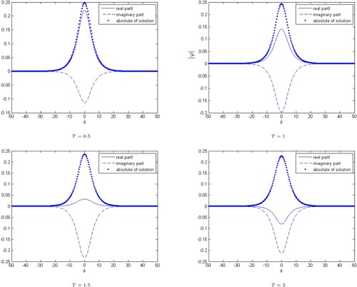
Table 1. The $E_{\mathrm{\infty }}$ at $\mathrm{\Delta }\tau =0.0001$, and T = 1 for Test Problem 1, where the convergence rate is 2 (see Theorem 4.1).

M	$E_{\mathrm{\infty }}$	Experimental rate of convergence
1	$9.9872\times {10}^{-2}$	–
2	$2.9424\times {10}^{-2}$	1.7630
4	$7.9739\times {10}^{-3}$	1.8836
8	$1.9021\times {10}^{-3}$	2.0676
16	$4.7361\times {10}^{-4}$	2.0058

Problem 2

In this case, we have considered the following linear problem to check the working performance of the proposed HWCM $\frac{{\mathrm{\partial }}^2\phi (t,\mathit{x})}{\mathrm{\partial }{t}^2}-\frac{{\mathrm{\partial }}^2\phi (t,\mathit{x})}{\mathrm{\partial }{x}^2}-\frac{{\mathrm{\partial }}^2\phi (t,\mathit{x})}{\mathrm{\partial }{y}^2}+3i\frac{\mathrm{\partial }\phi (t,\mathit{x})}{\mathrm{\partial }t}=0.$The initial and boundary information are $\begin{array}{rl}& \phi (0,x,y)=e^{(x+y)},\frac{\mathrm{\partial }\phi (0,x,y)}{\mathrm{\partial }t}=-i{e}^{(x+y)},(x,y)\in [0,1{]}^2,\\ & \phi (t,0,y)=e^{(y-it)},\phi (t,1,y)=e^{(1+y-it)},\phi (t,x,0)=e^{(x-it)},\phi (t,x,1)=e^{(x+1-it)}.\end{array}$The exact solution is $\phi (t,x,y)=e^{(x+y-it)}$. The numerical results are calculated at a different number of nodal points M in Table 2. Numerical solution with higher accuracy is also obtained by decreasing $\mathrm{\Delta }t$ and increasing M as highlighted in Table 3. The numerical solutions obtained by HWCM are compared with an exact solution at a portion of interval when x = y in Figure 2 and the absolute error in the entire domain is shown in Figure 3. These figures and tables are enough to demonstrate the proposed HWCM's efficiency and accuracy.

Figure 2. Comparison of exact and numerical solution at M = 16, T = 1 and $\mathrm{\Delta }t=0.0001$ for Test Problem 2 in the interval $[0,1{]}^2$.

Figure 3. The contour plot of absolute errors at M = 16, T = 1 and $\mathrm{\Delta }t=0.0001$ for Test Problem 2 in the interval $[0,1{]}^2$.

Table 2. The $E_{\mathrm{\infty }}$ and CPU time at various M with $\mathrm{\Delta }t=0.01$ and T = 1 for Test Problem 2.

M	$E_{\mathrm{\infty }}^{Re}$	$E_{\mathrm{\infty }}^{Im}$	$E_{\mathrm{\infty }}$	CPU time (second)
1	1.6935$\times {10}^{-2}$	6.8219$\times {10}^{-3}$	1.7181$\times {10}^{-2}$	1.0115
2	1.2570$\times {10}^{-2}$	8.9677$\times {10}^{-3}$	1.3673$\times {10}^{-2}$	1.5115
4	1.5602$\times {10}^{-2}$	8.4510$\times {10}^{-3}$	1.6359$\times {10}^{-2}$	1.8564
8	1.6039$\times {10}^{-2}$	7.9194$\times {10}^{-3}$	1.7314$\times {10}^{-2}$	2.1266
16	1.6474$\times {10}^{-2}$	7.9612$\times {10}^{-3}$	1.7674$\times {10}^{-2}$	4.5963

Table 3. The $E_{\mathrm{\infty }}$ and CPU time at various $\mathrm{\Delta }t$ with M = 16 and T = 1 for Test Problem 2.

$\mathrm{\Delta }t$	$E_{\mathrm{\infty }}^{Re}$	$E_{\mathrm{\infty }}^{Im}$	$E_{\mathrm{\infty }}$	CPU time (second)
0.1	3.1270$\times {10}^{-2}$	7.4856$\times {10}^{-2}$	7.6672$\times {10}^{-2}$	1.2486
0.01	1.6474$\times {10}^{-2}$	7.9612$\times {10}^{-3}$	1.7674$\times {10}^{-2}$	4.5963
0.001	4.5660$\times {10}^{-3}$	7.8935$\times {10}^{-4}$	4.6217$\times {10}^{-3}$	23.6887
0.0001	6.5115$\times {10}^{-4}$	8.9718$\times {10}^{-5}$	6.5725$\times {10}^{-4}$	60.6734
0.00001	6.6498$\times {10}^{-5}$	1.7532$\times {10}^{-5}$	6.7933$\times {10}^{-5}$	2645.6251

Problem 3

In this model example, we have considered the nonlinear homogeneous equation $\frac{{\mathrm{\partial }}^2\phi (t,\mathit{x})}{\mathrm{\partial }{t}^2}-\frac{{\mathrm{\partial }}^2\phi (t,\mathit{x})}{\mathrm{\partial }{x}^2}-\frac{{\mathrm{\partial }}^2\phi (t,\mathit{x})}{\mathrm{\partial }{y}^2}+i\frac{\mathrm{\partial }\phi (t,\mathit{x})}{\mathrm{\partial }t}+|\phi (t,\mathit{x}){|}^2\phi (t,x,y)+g\left(\mathit{x}\right)\phi (t,\mathit{x})=0.$The initial information is $\phi (0,x,y)=0\frac{\mathrm{\partial }\phi (0,x,y)}{\mathrm{\partial }t}=-i\sqrt{2}\pi \sin \left(\pi x\right)\sin \left(\pi y\right),\mathit{x}\in [a,b{]}^2,$where $g\left(\mathit{x}\right)={\sin }^2\left(\pi x\right){\sin }^2\left(\pi y\right)+\sqrt{2}\pi$ and the exact solution is $\phi (t,x,y)=\sin \left(\pi x\right)\sin \left(\pi y\right)e^{-i\sqrt{2}\pi t}$. The analytical solution can be used to determine the boundary conditions.

The numerical results are tested for different lengths of the intervals. In Figure 4, the numerical results along with the absolute error are displayed for the interval $[0,1]$. In Figure 5, the comparison of exact and numerical solutions are shown in term of contour plot, which are almost of the same patron in the interval $[-2,2]$. The oscillatory behaviour of the solution is visible in the 3-D view which is displayed in Figure 6 for the interval $[-2,2]$, which is difficult to capture accurately by traditional methods.

As the HWCM convergence rate is second order (see Theorem 4.2) which is supported by the numerical results, where we fixed $\mathrm{\Delta }t=0.0001$ and T = 1 in the interval $[0,1]$ for different values of M and the results in Table 4 are in line with the Theorem 4.2 that is second order of convergence.

Figure 4. The numerical results and the absolute error at M = 16, T = 5 and $\mathrm{\Delta }t=0.0001$ for Test Problem 3 in the interval $[0,1]$.

Figure 5. The exact and numerical solution at M = 16, T = 1 and $\mathrm{\Delta }t=0.001$ for Test Problem 3 in the interval $[-2,2]$.

Figure 6. The 3-D plot of solution at M = 16, T = 1 and $\mathrm{\Delta }t=0.001$ for Test Problem 3 in the interval $[-2,2]$.

Table 4. The $E_{\mathrm{\infty }}$ at $\mathrm{\Delta }t=0.0001$, and T = 1 for Test Problem 3 in the interval $[0,1]$. Theoretical rate of convergence is 2 (see Theorem 4.2).

M	$E_{\mathrm{\infty }}$	experimental rate of convergence
1	$8.7092\times {10}^{-2}$	–
2	$4.5820\times {10}^{-2}$	0.9265
4	$1.3571\times {10}^{-2}$	1.7554
8	$3.7333\times {10}^{-3}$	1.8206
16	$9.4255\times {10}^{-4}$	1.9858

Problem 4

In this last example, we solve the nonlinear challenging problem $\begin{array}{rl}& \frac{{\mathrm{\partial }}^2\phi (t,\mathit{x})}{\mathrm{\partial }{t}^2}-\frac{{\mathrm{\partial }}^2\phi (t,\mathit{x})}{\mathrm{\partial }{x}^2}-\frac{{\mathrm{\partial }}^2\phi (t,\mathit{x})}{\mathrm{\partial }{y}^2}+i\frac{\mathrm{\partial }\phi (t,\mathit{x})}{\mathrm{\partial }t}+|\phi (t,\mathit{x}){|}^2\phi (t,x,y)=0,\\ & \mathit{x}\in [-25,25{]}^2,\end{array}$

with homogeneous Dirichlet type boundary conditions along with the following initial conditions $\phi (0,x,y)=(x+y)(i+1)e^{-10(1-x-y{)}^2},\frac{\mathrm{\partial }\phi (0,x,y)}{\mathrm{\partial }t}=0.$

The analytical solution of this problem is not defined. Due to the soliton wave's blow-up phenomenon, this problem is complicated, and been considered a challenging case of Schrödinger equation in many articles [16, 77].

We utilize the HWCM, presented in this research to replicate this challenging problem and it has accurately captured the moving soliton seen from Figures 7–9. In Figure 7, we show the soliton $|\phi |$ movement in a section views when x = y to clearly explain the applicability of the scheme.

Figure 7. The propagation of soliton wave at different T with M = 16 and $\mathrm{\Delta }t=0.01$ for Test Problem 4 in the interval $[-25,25]$.

The movement of soliton wave is shown in Figure 8 at various T, where the propagation of the soliton is clearly visible as time passes from the contour plot (from $T=1$ to T = 12). Further illustration can be also seen in Figure 9, where the soliton wave swiftly converts into lower waves and that additional ripples appear as the wave progresses and the single soliton splits into several little solitons and moves furiously as the time increases. The smoothness of the curves in Figure 9 as compare to Figure 7 is due to the use of much collocation points (M = 128). So by increasing the collocation points M, the accuracy can be increased of the proposed HWCM. From these figures, it is obvious that the numerical findings are accurate and stable and do not reflect the blow-up phenomena because we have introduced a multi-resolution procedure based on Haar function to solve nonlinear Schrödinger equation with wave operator.

Figure 8. The propagation of soliton wave at different T with M = 16 and $\mathrm{\Delta }t=0.01$ for Test Problem 4 in the interval $[-25,25]$.

Figure 9. The propagation of soliton wave at different T with M = 128 and $\mathrm{\Delta }t=0.01$ for Test Problem 4 in the interval $[-32,32]$.

6. Stability

We investigate the system of linear Equations (26(26) $\begin{array}{rl}& \sum _{\ell =1}^{2M}\sum _{i=1}^{2M}{a}_{i\ell }^{M,n+1}\left\{(1+i\frac{\mathrm{\Delta }t}{2}\alpha +\frac{\mathrm{\Delta }{t}^2(g(x_l,y_s)+\text{β}(x_l,y_s)|H_{M_l^s}^n{|}^2)}{2}){\tilde{h}}_i\right(x_l\left)h_{\ell }\right(y_s)\\ & -\mathrm{\Delta }{t}^2{h}_i\left(x_l\right)h_{\ell }\left(y_s\right)\phantom{(1+i\frac{\mathrm{\Delta }t}{2}\alpha +\frac{\mathrm{\Delta }{t}^2(g(x_l,y_s)+\text{β}(x_l,y_s)|H_{M_l^s}^n{|}^2)}{2})}\}-\sum _{\ell =1}^{2M}\sum _{i=1}^{2M}{b}_{i\ell }^{M,n+1}\{\mathrm{\Delta }{t}^2{h}_i\left(x_l\right)h_{\ell }\left(y_s\right)\}\\ & =(2+i\frac{\mathrm{\Delta }t}{2}\alpha -\frac{\mathrm{\Delta }{t}^2(g(x_l,y_s)+\text{β}(x_l,y_s)|H_{M_l^s}^n{|}^2)}{2})H_{M_l^s}^n-H_{M_l^s}^{n-1}.\end{array}$(26) ) and (27(27) $\begin{array}{rl}\sum _{\ell =1}^{2M}\sum _{i=1}^{2M}{a}_{i\ell }^{M,n+1}{\tilde{h}}_i\left(x_l\right)h_{\ell }\left(y_s\right)& -\sum _{\ell =1}^{2M}\sum _{i=1}^{2M}{b}_{i\ell }^{M,n+1}{h}_i\left(x_l\right){\tilde{h}}_{\ell }\left(y_s\right)\\ & ={\tilde{\phi }}_l(x_l,y_s,t_{n+1})-{\tilde{\phi }}_o(x_l,y_s,t_{n+1}).\end{array}$(27) ), which are the main system to test the computational stability of the proposed HWCM and can be presented as $H\mathcal{X}=B.$

The associated Haar weights are denoted by the matrix H, the vector of unknown constant based on approximation is represented by $\mathcal{X}$ and B is the known vector. To observe the stability computationally we used the following definition.

Definition 6.1

[78]

Assume that a numerical approach for solving a differential equation gives a sequence of matrix equations of the type $H\mathcal{X}=\mathcal{B}$. If the inverse of H exists and is bounded then we say that the procedure is stable i.e. $\Vert H^{-1}\Vert \le C,$where C is some constant.

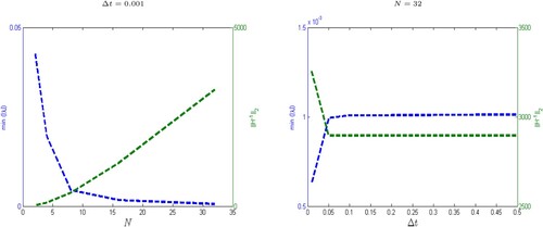
Following the above definition of stability, the smallest value of the magnitudes of the eigenvalues of H is calculated numerically for Test Problem 2–3, which reflects the magnitude of the spectral radius of $H^{-1}$ (see Figures 10 and 11). We also observe from Figures 10 and 11 that the 2-norm of $H^{-1}$ do not grow too quickly by increasing N = 2M and decreasing $\mathrm{\Delta }t$ at fixed T. Hence, the proposed Haar wavelet schemes are reasonably stable.

Figure 10. Spectral radius of $H^{-1}$ and the 2-norm of $H^{-1}$ at T = 1 for Test Problem 2.

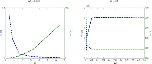
Figure 11. Spectral radius of $H^{-1}$ and the 2-norm of $H^{-1}$ at T = 1 for Test Problem 3.

7. Conclusion

In this study, we propose a HWCM for the numerical investigation of two-dimensional NHSEs. The HWCM captures not only the accurate solution of NHSE but also closely reflects the movement and propagation of soliton waves in a straight forward manner. As the time increases, the soliton wave swiftly converts into lower waves and that additional ripples appear as the wave progresses and the single soliton splits into several little solitons and moves furiously. The blow-up phenomenon has also been handled by the HWCM in NHSEs without any difficulty. The theoretical rate of convergence which is the important part of this study is in-line with the experimental rate of convergence and has been highlighted for different cases in many tables. The HWCM is accurate and appropriate to solving NHSEs, as evidenced by the $E_{\mathrm{\infty }}$ error norm and rate of convergence.

Based on the above performed numerical tests and the implementation of HWCM on various types of nonlinear equations, we can infer that the proposed HWCM is feasible, efficient and effective for solving NHSEs. The HWCM has been implemented for NHSE with square domain and can be modified for rectangular domain without any complexity but it is difficult to implement on irregular domains. The proposed method can be extended to the system of NHSEs with different types of boundary condition, because of the HWCM's tremendous potential accomplishments presented in this paper. These issues will be the main focus of our future studies.

Author Contributions

All authors contributed equally to finalized this manuscript. All authors read and approved the final manuscript.

Disclosure statement

No potential conflict of interest was reported by the author(s).

Data Availability

The datasets generated and analysed during the current study are included in this paper.

References

- Newell AC. Solitons in mathematics and physics. Philadelphia, PA: SIAM; 1985.
- Keller JB, Papadakis JS. Wave propagation and underwater acoustics. Vol. 70. Springer; 1977.
- Hasegawa A, Kodama Y. Solitons in Optical communications. Oxford: Clarendon Press; 1995.
- Ablowitz MJ, Segur H. Solitons and the inverse scattering transform. Philadelphia: SIAM; 1981.
- Antoine X, Bao W, Besse C. Computational methods for the dynamics of the nonlinear Schrödinger/Gross–Pitaevskii equations. Comput Phys Commun. 2013;184(12):2621–2633.
- Cai W, He D, Pan K. A linearized energy–conservative finite element method for the nonlinear Schrödinger equation with wave operator. Appl Numer Math. 2019;140:183–198.
- Frassu S, Rodríguez Galván R, Viglialoro G. Uniform in time L∞-estimates for an attraction-repulsion chemotaxis model with double saturation. Discrete Continuous Dyn Systems-Series B. 2022;28(3):1886–1904.
- Frassu S, Li T, Viglialero G. Improvements and generalizations of results concerning attraction repulsion chemotaxis models. Math Methods Appl Sci. 2022;45(17):11067–11078.
- Pervaiz N, Aziz I. Haar wavelet approximation for the solution of cubic nonlinear Schrödinger equations. Physica A: Statist Mechan Appl. 2020;545:123738.
- Brugnano L, Zhang C, Li D. A class of energy-conserving hamiltonian boundary value methods for nonlinear Schrödinger equation with wave operator. Commun Nonlinear Sci Numerical Simul. 2018;60:33–49.
- Singh J, Kumar D. Numerical study for time-fractional Schrödinger equations arising in quantum mechanics. Nonlinear Eng. 2014;3(3):169–177.
- Li X, Zhang L, Zhang T. A new numerical scheme for the nonlinear Schrödinger equation with wave operator. Journal of Applied Mathematics and Computing. 2017;54(1-2):109–125.
- Wang T, Guo B. Unconditional convergence of two conservative compact difference schemes for non-linear Schrödinger equation in one dimension. Scientia Sinica Math. 2011;41(3):207–233.
- Samira L, Omrani K. A new conservative fourth-order accurate difference scheme for the nonlinear Schrödinger equation with wave operator. Appl Numer Math. 2021;173:1–12.
- Wang S, Zhang L, Fan R. Discrete-time orthogonal spline collocation methods for the nonlinear Schrödinger equation with wave operator. J Comput Appl Math. 2011;235(8):1993–2005.
- Guo L, Xu Y. Energy conserving local discontinuous Galerkin methods for the nonlinear Schrödinger equation with wave operator. J Sci Comput. 2015;65(2):622–647.
- Wang L, Kong L, Zhang L, et al. Multi-symplectic preserving integrator for the Schrödinger equation with wave operator. Appl Math Modell. 2015;39(22):6817–6829.
- Ji B, Zhang L. An exponential wave integrator Fourier pseudospectral method for the nonlinear Schrödinger equation with wave operator. J Appl Math Comput. 2018;58(1-2):273–288.
- Li S, Wang T, Wang J, et al. An efficient and accurate Fourier pseudo-spectral method for the nonlinear Schrödinger equation with wave operator. Int J Comput Math. 2021;98(2):340–356.
- Wang T, Zhang L. Analysis of some new conservative schemes for nonlinear Schrödinger equation with wave operator. Appl Math Comput. 2006;182(2):1780–1794.
- Yang Y, Li H, Guo X. A linearized energy-conservative scheme for two-dimensional nonlinear Schrödinger equation with wave operator. Appl Math Comput. 2021;404:126234.
- Guo B, Li H. On the problem of numerical calculation for a class of the system of nonlinear Schrödinger equations with wave operator. J Numerical Methods Computer Appl. 1983;4:258–263.
- Li H. Local absorbing boundary conditions for two-dimensional nonlinear Schrödinger equation with wave operator on unbounded domain. Math Methods Appl Sci. 2021;44(18):14382–14392.
- Liu X, Ahsan M, Ahmad M, et al. Applications of Haar wavelet-finite difference hybrid method and its convergence for hyperbolic nonlinear Schrödinger equation with energy and mass conversion. Energies. 2021;14(23):7831.
- Karakashian O, Akrivis GD, Dougalis VA. On optimal order error estimates for the nonlinear schrödinger equation. SIAM J Numer Anal. 1993;30(2):377–400.
- Wu L. DuFort–Frankel-type methods for linear and nonlinear Schrödinger equations. SIAM J Numer Anal. 1996;33(4):1526–1533.
- Bao W, Jin S, Markowich PA. Numerical study of time-splitting spectral discretizations of nonlinear Schrödinger equations in the semiclassical regimes. SIAM J Sci Comput. 2003;25(1):27–64.
- Taleei A, Dehghan M. Time-splitting pseudo-spectral domain decomposition method for the soliton solutions of the one-and multi-dimensional nonlinear Schrödinger equations. Comput Phys Commun. 2014;185(6):1515–1528.
- Arico A, Rodriguez G, Seatzu S. Numerical solution of the nonlinear Schrödinger equation, starting from the scattering data. Calcolo. 2011;48(1):75–88.
- Duan Y, Rong F. A numerical scheme for nonlinear Schrödinger equation by MQ quasi-interpolation. Eng Anal Bound Elem. 2013;37(1):89–94.
- Wang T, Guo B, Xu Q. Fourth-order compact and energy conservative difference schemes for the nonlinear Schrödinger equation in two dimensions. J Comput Phys. 2013;243:382–399.
- Doha EH, Bhrawy AH, Abdelkawy MA, et al. Jacobi–Gauss–Lobatto collocation method for the numerical solution of 1 + 1 nonlinear Schrödinger equations. J Comput Phys. 2014;261:244–255.
- Bashan A, Yagmurlu NM, Ucar Y, et al. An effective approach to numerical soliton solutions for the Schrödinger equation via modified cubic B-spline differential quadrature method. Chaos, Solitons & Fractals. 2017;100:45–56.
- Li H, Wang Y. An averaged vector field legendre spectral element method for the nonlinear Schrödinger equation. Int J Comput Math. 2017;94(6):1196–1218.
- Gao W, Ismael HF, Husien AM, et al. Optical soliton solutions of the cubic-quartic nonlinear Schrödinger and resonant nonlinear Schrödinger equation with the parabolic law. Appl Sci. 2020;10(1):219.
- Seadawy AR. Modulation instability analysis for the generalized derivative higher order nonlinear Schrödinger equation and its the bright and dark soliton solutions. J Electromagnetic Waves Appl. 2017;31(14):1353–1362.
- Ali A, Seadawy AR, Lu D. Soliton solutions of the nonlinear Schrödinger equation with the dual power law nonlinearity and resonant nonlinear Schrödinger equation and their modulation instability analysis. Optik. 2017;145:79–88.
- Arshed S, Arif A. Soliton solutions of higher-order nonlinear Schrödinger equation (NLSE) and nonlinear Kudryashov's equation. Optik. 2020;209:164588.
- Yang J, Tian S, Peng W, et al. The N-coupled higher-order nonlinear Schrödinger equation: Riemann-Hilbert problem and multi-soliton solutions. Math Methods Appl Sci. 2020;43(5):2458–2472.
- Osman M, Ali KK, Gómez-Aguilar J. A variety of new optical soliton solutions related to the nonlinear Schrödinger equation with time-dependent coefficients. Optik. 2020;222:165389.
- Riaz MB, Atangana A, Jhangeer A, et al. Soliton solutions, soliton-type solutions and rational solutions for the coupled nonlinear Schrödinger equation in magneto-optic waveguides. Eur Phys J Plus. 2021;136(2):1–19.
- Awan A, Rehman H, Tahir M, et al. Optical soliton solutions for resonant Schrödinger equation with anti-cubic nonlinearity. Optik. 2021;227:165496.
- Tchaho C, Omanda H, Mbourou G, et al. Hybrid dispersive optical solitons in nonlinear cubic-quintic-septic schrödinger equation. Opt Photonics J. 2021;11(2):23–49.
- Herzallah MA, Gepreel KA. Approximate solution to the time–space fractional cubic nonlinear Schrödinger equation. Appl Math Model. 2012;36(11):5678–5685.
- Secchi S, Squassina M. Soliton dynamics for fractional Schrödinger equations. Appl Anal. 2014;93(8):1702–1729.
- Yousif E, Abdel-Salam E-B, El-Aasser M. On the solution of the space-time fractional cubic nonlinear Schrödinger equation. Res Phys. 2018;8:702–708.
- Wang P, Huang C. A conservative linearized difference scheme for the nonlinear fractional Schrödinger equation. Numer Algorithms. 2015;69(3):625–641.
- Abdel-Salam EA, Yousif EA, El-Aasser MA. Analytical solution of the space-time fractional nonlinear Schrödinger equation. Rep Math Phys. 2016;77(1):19–34.
- Liu Y, Liu Y, Cen Z. Daubechies wavelet meshless method for 2-D elastic problems. Tsinghua Sci Technol. 2008;13(5):605–608.
- Díaz LA, Martín MT, Vampa V. Daubechies wavelet beam and plate finite elements. Finite Elements Anal Design. 2009;45(3):200–209.
- Jang G, Kim Y, Choi K. Remesh-free shape optimization using the wavelet-Galerkin method. Int J Solids Structures. 2004;41(22):6465–6483.
- Aziz I, Al-Fhaid AS. An improved method based on Haar wavelets for numerical solution of nonlinear integral and integro-differential equations of first and higher orders. J Comput Appl Math. 2014;260:449–469.
- Ahsan M, Hussain I. A multi-resolution collocation procedure for time-dependent inverse heat problems. Int J Thermal Sci. 2018;128:160–174.
- Ahsan M, Hussain I. Haar wavelets multi-resolution collocation analysis of unsteady inverse heat problems. Inverse Probl Sci Eng. 2019;27(11):1498–1520.
- Dahmen W, Kurdila AJ, Oswald P. Multiscale wavelet methods for partial differential equations. Aachen, Germany: Elsevier; 1997. (Wavelet Analysis and its Applications; 6).
- Tran T, Stephan EP, Mund P. Hierarchical basis preconditioners for first kind integral equations. Appl Anal. 1997;65(3–4):353–372.
- Aziz I, Khan W. Numerical integration of multi-dimensional highly oscillatory, gentle oscillatory and non-oscillatory integrands based on wavelets and radial basis functions. Eng Anal Boundary Elements. 2012;36(8):1284–1295.
- Lepik U. Numerical solution of evolution equations by the Haar wavelet method. Appl Math Comput. 2007;185(1):695–704.
- Hsiao C, Wang W. Haar wavelet approach to nonlinear stiff systems. Math Comput Simul. 2001;57(6):347–353.
- Ahsan M, Bohner M, Ullah A, et al. A Haar wavelet multi-resolution collocation method for singularly perturbed differential equations with integral boundary conditions. Math Comput Simul. 2023;204:166–180.
- Majak J, Pohlak M, Karjust K, et al. New higher order Haar wavelet method: application to FGM structures. Compos Struct. 2018;201:72–78.
- Ahsan M, Tran T, Hussain I. A multiresolution collocation method and its convergence for Burgers' type equations. Math Methods Appl Sci. 2022:1–24. DOI:10.002/mma.8764
- Majak J, Shvartsman B, Pohlak M, et al. Solution of fractional order differential equation by the Haar wavelet method. Numerical convergence analysis for most commonly used approach. In: AIP Conference Proceedings, Vol. 1738, AIP Publishing LLC; 2016. p. 480110.
- Li Y, Zhao W. Haar wavelet operational matrix of fractional order integration and its applications in solving the fractional order differential equations. Appl Math Comput. 2010;216(8):2276–2285.
- Yi M, Huang J. Wavelet operational matrix method for solving fractional differential equations with variable coefficients. Appl Math Comput. 2014;230:383–394.
- Saeed U, Rehman M. Haar wavelet picard method for fractional nonlinear partial differential equations. Appl Math Comput. 2015;264:310–322.
- Wang L, Ma Y, Meng Z. Haar wavelet method for solving fractional partial differential equations numerically. Appl Math Comput. 2014;227:66–76.
- Nazir S, Shahzad S, Wirza R, et al. Birthmark based identification of software piracy using Haar wavelet. Math Comput Simul. 2019;166:144–154.
- Ahsan M, Shams-ul-Haq K, Liu X, et al. A Haar wavelets based approximation for nonlinear inverse problems influenced by unknown heat source. Math Methods Appl Sci. 2022;46(230):2475–2487.
- Ahsan M, Hussain I, Ahmad M. A finite-difference and Haar wavelets hybrid collocation technique for non-linear inverse Cauchy problems. Appl Math Sci Eng. 2022;30(1):121–140.
- Ahsan M, Lin S, Ahmad M, et al. A Haar wavelet-based scheme for finding the control parameter in nonlinear inverse heat conduction equation. Open Phys. 2021;19(1):722–734.
- Ahsan M, Lei W, Ahmad M, et al. A wavelet-based collocation technique to find the discontinuous heat source in inverse heat conduction problems. Phys Scripta. 2022;9:125208.
- Ahsan M, Ahmad I, Ahmad M, et al. A numerical Haar wavelet-finite difference hybrid method for linear and non-linear Schrödinger equation. Math Comput Simul. 2019;165:13–25.
- Liu X, Ahsan M, Ahmad M, et al. Haar wavelets multi-resolution collocation procedures for two-dimensional nonlinear Schrödinger equation. Alexandria Eng J. 2021;60(3):3057–3071.
- Majak J, Shvartsman B, Kirs M, et al. Convergence theorem for the Haar wavelet based discretization method. Compos Struct. 2015;126:227–232.
- Arbabi S, Nazari A, Darvishi MT. A two-dimensional Haar wavelets method for solving systems of PDEs. Appl Math Comput. 2017;292:33–46.
- Li X, Gong Y, Zhang L. Linear high-order energy-preserving schemes for the nonlinear Schrödinger equation with wave operator using the scalar auxiliary variable approach. J Sci Comput. 2021;88(1):1–25.
- LeVeque RJ. Finite difference methods for ordinary and partial differential equations. Philadelphia: Society for Industrial and Applied Mathematics; 2007.