Optimal control analysis of coffee berry borer infestation in the presence of farmer's awareness

Abstract

Coffee is the most critical stimulant beverage in the world and represents a significant source of income in many tropical and subtropical countries. In this paper, a deterministic mathematical model has been formulated to describe the infestation dynamic of coffee berry borer (CBB) using a system of non-linear ordinary differential equations with farmers' awareness and optimal control. The system has two equilibrium points, namely the CBB free equilibrium point and the endemic equilibrium point which exist conditionally. The basic reproduction number, which plays a vital role in mathematical epidemiology, was derived. The qualitative analysis of the model revealed the scenario for both CBB free equilibrium and endemic equilibrium points. The local stability of the equilibria is established via the Jacobian matrix and Routh–Hurwitz criteria, while the global stability of the equilibria is proven by using an appropriate Lyapunov function. The normalized sensitivity analysis has also been performed to observe the impact of different parameters on the basic reproduction number. We extended the proposed model into an optimal control problem by incorporating two control variables, the effort made to reduce the colonizing females based on chemicals, traps, and biological control using entomopathogenic fungi such as Beauveria bassiana, that are applied to the surface of the coffee berries and kill the colonizing females of CBB when they drill an entry hole into the coffee berry and the effort made to increase the awareness of farmers through media campaign and education for the coffee farmer. Then the optimal control strategy is found by minimizing the number of CBB individuals considering the cost of implementation. The existence of optimal controls is examined using Pontryagin's minimum principle. Finally, the numerical simulations show agreement with the analytical results.

Keywords:

• Hypothenemus hampei
• Farmers' awareness
• sensitivity analysis
• optimal control
• numerical simulation

Mathematics Subject Classifications:

• 92C60
• 68Q07
• 34-00

1. Introduction

Coffee is the most critical stimulant beverage in the world and represent a significant source of income in many tropical and subtropical countries. It is produced in more than 80 countries and is worth about $24 billion from exports [1]. Globally, in producing and consuming countries, coffee is an important commodity [2]. Coffee production is affected by several pests, weeds and diseases. Among these pests, coffee berry borer (CBB), Hypothenemus hampei was the most harmful pest that affects commercial coffee production and prevalent in most coffee-producing countries [3]. Antestia bug and coffee blotch miner also widely damage the production of coffee [4].

CBB was first reported in Gabon (1901), and soon after in Kenya in 1928 [5]. Later, it had quickly spread throughout most all the 80 coffee-producing countries [6]. CBB is a pest that harms immature and mature coffee berries without damaging leaves, branches, and stems. The female CBB drills the apex of the coffee berry eats and oviposit inside the coffee berry. The larvae also feed on the same seed until they grow and reach the adult stage. Mature females are responsible for the dispersal of the population: they emerge from the berries to colonize and lay their eggs in new berries, while males and larvae stages remain inside the berries [5]. It damages the weight and quality because it feeds and reproduces inside the coffee berry [7]. Sibling mating inside the coffee berry makes this pest quite difficult to control.

The infestation intensity of CBB in coffee-growing countries is reported as Mexico 60%, Malaysia 50–90%, Colombia 60%, Jamaica 75%, Uganda 80%, and Tanzania 90% [2]. Due to the intensity of the damages, several control methods have been identified and implemented in most coffee-growing countries. The common control methods are improved cultural practices, chemical, biological control, and host plant resistance [8–10]. Moreover, adopting the integrated application of new technologies like television, radio, and mobile telephony provides useful information about pest outbreaks and crop protection during agricultural pest control awareness programmes [11,12].

Mathematical modelling has a crucial role in better understanding the dynamics of plant disease and its control. The literature on the application of mathematical modelling in the area of plant disease is extensive, see for example in [13–21] and references cited therein. In [22], Fotsa et al. introduced and analysed a dynamical spatial model of Anthracnose infection that include optimal control. Anthracnose is another name for CBD. They also showed how to optimize the use of chemical control with respect to a given cost function. Later, this study was generalized by incorporating an impulsive control strategy that represents cultivation practices in [23]. Farmers' awareness plays a significant role in the management of pests, see for example in [24–26]. However, farmers awareness was not considered in these literatures for CBB. This is will be addressed in the present study. Cunniffe and Gilligan [27] investigated an epidemiological model for plant pathogens. This model ensured maximum transferability across the widest range of host–pathogen systems by using the common currency of the field and has illustrated the results in a class of models that have been experimentally tested for plant disease.

The aim of this study is to provide quantitative and qualitative explanations for the dynamics of CBB infestation by taking into account vectors' population and farmers' awareness. For this, we propose a nonlinear deterministic mathematical model to investigate the dynamics of CBB infestation in the presence of farmers' awareness. Also, we extend the proposed model into an optimal control problem.

The rest of this work is organized as follows. In Section 2, a mathematical model for CBB infestation is derived. The stability analysis of the proposed model is investigated in Section 3. Section 4 deals with the extended mathematical model into an optimal control problem. The obtained analytical results are shown through numerical simulations in Section 5. Cost-effectiveness analysis is discussed in Section 6. Finally, conclusions are drawn in Section 7.

2. Model derivation

In this section, we consider a mathematical model proposed by Abawari [28] to study the infestation dynamics of CBB. In the model, we introduce coffee berry biomass (B), coffee borer population (Y ), and aware farmers (A). Due to the limit size of coffee plantations, however it may be large, we assume logistic growth for the biomass of coffee plant [29], with growth rate r and carrying capacity k. The female CBB attacks immature and mature coffee berries from about eight weeks after flowering up to harvest season. We assumed that females bore a hole into the coffee berry and then construct galleries in the seeds where the eggs are deposited, followed by larval feeding on the coffee seed [30]. The main coffee borer management measures involve different components, including regular monitoring, controlled harvest, and the use of biological control agents. These measures are useful before the females enter the coffee berries. Once, it entered the coffee berries it is difficult to control the pest [2]. Thus, we assumed that infected female bores do not affect the coffee berries. This is due to its lack of power to drill into coffee berries. The natural death rate of coffee berry is denoted by μ. The female borer dies at a rate d.

The per capita rate at which a female borer attacks coffee berry is represented by $\gamma B/(c+B)$. Here, γ represents the attack rate of a female borer on coffee berries while c represents the half-saturation constant. Then the founder female remains inside the fruit after oviposition until she dies, taking care of the offspring. Hence, when the new adult females emerge, they are already inseminated and ready to attack another coffee berry, in which they continue the cycle. Most of the life cycle occurs inside the coffee berry.

The farmer awareness measures the information density available among the farmers due to the prevalence of the CBB. It is assumed to increase due to media campaigns and agricultural field workers. We assumed that the rate of farmers' awareness is proportional to the infestation burden and increases with rate α. As a result of awareness farmers surveillance their farm, and use biological control or trap to avoid borer infestation. There is a farmers' activity rate, β, due to self-aware human inter- actions and activity such as the use of bio-pesticides, modelled via the mass action term $\text{β}AY/(\delta +A)$. Here, δ is the constant related to saturation in information-induced intervention. We also assumed farmers' memory faded and thus, the level of awareness decreased at a rate e.

Based on the above assumptions, the mathematical model is described by nonlinear systems of ordinary differential equations: (1) $\begin{array}{rl}{\displaystyle \frac{\mathrm{d}B}{\mathrm{d}t}}& =rB(1-{\displaystyle \frac{B}{k}})-{\displaystyle \frac{\gamma BY}{c+B}}-\mu B,\\ {\displaystyle \frac{\mathrm{d}Y}{\mathrm{d}t}}& ={\displaystyle \frac{\sigma \gamma BY}{c+B}}-{\displaystyle \frac{\text{β}AY}{\delta +A}}-\mathrm{d}Y,\\ {\displaystyle \frac{\mathrm{d}A}{\mathrm{d}t}}& =\theta +\alpha Y-eA,\end{array}$(1) where $B\left(0\right)=B_0>0,Y\left(0\right)=Y_0\ge 0,A\left(0\right)=A_0\ge 0$.

Here σ and θ denote conversion rate and rate of awareness due to global source, respectively. Compared to the mathematical model introduced in [11], the present model differs due to the logistic growth model and farmer's awareness being included.

3. Model analysis

3.1. Positivity and boundedness of solutions

In this section, we study a region in which the solution of the governing system (1(1) $\begin{array}{rl}{\displaystyle \frac{\mathrm{d}B}{\mathrm{d}t}}& =rB(1-{\displaystyle \frac{B}{k}})-{\displaystyle \frac{\gamma BY}{c+B}}-\mu B,\\ {\displaystyle \frac{\mathrm{d}Y}{\mathrm{d}t}}& ={\displaystyle \frac{\sigma \gamma BY}{c+B}}-{\displaystyle \frac{\text{β}AY}{\delta +A}}-\mathrm{d}Y,\\ {\displaystyle \frac{\mathrm{d}A}{\mathrm{d}t}}& =\theta +\alpha Y-eA,\end{array}$(1) ) is both epidemiologically and mathematically meaningful. That is, the solution of the proposed model is nonnegative and bounded with positive initial data in a certain feasible region. Now we have the following theorem.

Theorem 3.1

If the initial data $\left(B\right(0),Y(0),A(0)\in {\mathbb{R}}_{+}^3)$, then the solutions $\left(B\right(t),Y(t),A(t\left)\right)$ of the system (1(1) $\begin{array}{rl}{\displaystyle \frac{\mathrm{d}B}{\mathrm{d}t}}& =rB(1-{\displaystyle \frac{B}{k}})-{\displaystyle \frac{\gamma BY}{c+B}}-\mu B,\\ {\displaystyle \frac{\mathrm{d}Y}{\mathrm{d}t}}& ={\displaystyle \frac{\sigma \gamma BY}{c+B}}-{\displaystyle \frac{\text{β}AY}{\delta +A}}-\mathrm{d}Y,\\ {\displaystyle \frac{\mathrm{d}A}{\mathrm{d}t}}& =\theta +\alpha Y-eA,\end{array}$(1) ) are non-negative for all time $t\ge 0$ and bounded. Moreover, the feasible compact set is given by $\begin{array}{rl}\mathrm{\Omega }& =\left\{\right(B,Y,A)\in {\mathbb{R}}_{+}^3:0<B\le k,0<Y\le {\displaystyle \frac{M(\sigma r+1)}{\xi }}-\sigma k,\\ & 0\le A\le {\displaystyle \frac{\xi \theta +\alpha M(\sigma r+1)}{e\xi }}\},\end{array}$where $M=max\left\{B\right(0),k\}$ and $\xi =min\{1,d\}$.

Proof.

From the first equation system (1(1) $\begin{array}{rl}{\displaystyle \frac{\mathrm{d}B}{\mathrm{d}t}}& =rB(1-{\displaystyle \frac{B}{k}})-{\displaystyle \frac{\gamma BY}{c+B}}-\mu B,\\ {\displaystyle \frac{\mathrm{d}Y}{\mathrm{d}t}}& ={\displaystyle \frac{\sigma \gamma BY}{c+B}}-{\displaystyle \frac{\text{β}AY}{\delta +A}}-\mathrm{d}Y,\\ {\displaystyle \frac{\mathrm{d}A}{\mathrm{d}t}}& =\theta +\alpha Y-eA,\end{array}$(1) ), we have (2) ${\displaystyle \frac{\mathrm{d}B}{\mathrm{d}t}}\ge -(\gamma +\mu )B.$(2) Integrating Equation (2(2) ${\displaystyle \frac{\mathrm{d}B}{\mathrm{d}t}}\ge -(\gamma +\mu )B.$(2) ), we obtain $B\left(t\right)\ge B\left(0\right){\mathrm{e}}^{-(\gamma +\mu )t}>0.$Similarly, from the second and third equations of system (1(1) $\begin{array}{rl}{\displaystyle \frac{\mathrm{d}B}{\mathrm{d}t}}& =rB(1-{\displaystyle \frac{B}{k}})-{\displaystyle \frac{\gamma BY}{c+B}}-\mu B,\\ {\displaystyle \frac{\mathrm{d}Y}{\mathrm{d}t}}& ={\displaystyle \frac{\sigma \gamma BY}{c+B}}-{\displaystyle \frac{\text{β}AY}{\delta +A}}-\mathrm{d}Y,\\ {\displaystyle \frac{\mathrm{d}A}{\mathrm{d}t}}& =\theta +\alpha Y-eA,\end{array}$(1) ), we get $Y\left(t\right)\ge Y\left(0\right){\mathrm{e}}^{-(\text{β}+d)t}\ge 0\mathrm{a}\mathrm{n}\mathrm{d}A\left(t\right)\ge A\left(0\right){\mathrm{e}}^{-et}\ge 0,$respectively. This implies that all the solution with positive initial data remains in ${\mathbb{R}}_{+}^3$ for all $t\ge 0$. This means, the region attracts all solutions of the governing system.

Next, we determine the feasible region in which the solution of the model (1(1) $\begin{array}{rl}{\displaystyle \frac{\mathrm{d}B}{\mathrm{d}t}}& =rB(1-{\displaystyle \frac{B}{k}})-{\displaystyle \frac{\gamma BY}{c+B}}-\mu B,\\ {\displaystyle \frac{\mathrm{d}Y}{\mathrm{d}t}}& ={\displaystyle \frac{\sigma \gamma BY}{c+B}}-{\displaystyle \frac{\text{β}AY}{\delta +A}}-\mathrm{d}Y,\\ {\displaystyle \frac{\mathrm{d}A}{\mathrm{d}t}}& =\theta +\alpha Y-eA,\end{array}$(1) ) is bounded. Let us consider the first equation of system (1(1) $\begin{array}{rl}{\displaystyle \frac{\mathrm{d}B}{\mathrm{d}t}}& =rB(1-{\displaystyle \frac{B}{k}})-{\displaystyle \frac{\gamma BY}{c+B}}-\mu B,\\ {\displaystyle \frac{\mathrm{d}Y}{\mathrm{d}t}}& ={\displaystyle \frac{\sigma \gamma BY}{c+B}}-{\displaystyle \frac{\text{β}AY}{\delta +A}}-\mathrm{d}Y,\\ {\displaystyle \frac{\mathrm{d}A}{\mathrm{d}t}}& =\theta +\alpha Y-eA,\end{array}$(1) ) (3) ${\displaystyle \frac{\mathrm{d}B}{\mathrm{d}t}}=rB(1-{\displaystyle \frac{B}{k}})-{\displaystyle \frac{\gamma BY}{c+B}}-\mu B\le rB(1-{\displaystyle \frac{B}{k}}).$(3) Integrating the last inequality of Equation (3(3) ${\displaystyle \frac{\mathrm{d}B}{\mathrm{d}t}}=rB(1-{\displaystyle \frac{B}{k}})-{\displaystyle \frac{\gamma BY}{c+B}}-\mu B\le rB(1-{\displaystyle \frac{B}{k}}).$(3) ) by separation of variables, we obtain $B\left(t\right)\le {\displaystyle \frac{kB\left(0\right)}{{\mathrm{e}}^{-rt}(k+B(0\left)\right)+B\left(0\right)}}.$From which we deduce that $B\left(t\right)\le k$ and we have $\overline{lim}B\left(t\right)\le k$.

Let $w=\sigma B+Y$ at any time t and $\xi =min\{1,d\}$, then by adding the first and second equation of system (1(1) $\begin{array}{rl}{\displaystyle \frac{\mathrm{d}B}{\mathrm{d}t}}& =rB(1-{\displaystyle \frac{B}{k}})-{\displaystyle \frac{\gamma BY}{c+B}}-\mu B,\\ {\displaystyle \frac{\mathrm{d}Y}{\mathrm{d}t}}& ={\displaystyle \frac{\sigma \gamma BY}{c+B}}-{\displaystyle \frac{\text{β}AY}{\delta +A}}-\mathrm{d}Y,\\ {\displaystyle \frac{\mathrm{d}A}{\mathrm{d}t}}& =\theta +\alpha Y-eA,\end{array}$(1) ), we obtain $\begin{array}{rl}{w}^{\prime }& =\sigma B^{\prime }+Y^{\prime }\\ & =\sigma rB(1-{\displaystyle \frac{B}{k}})-\sigma {\displaystyle \frac{\gamma BY}{c+B}}-\sigma \mu B+\sigma {\displaystyle \frac{\gamma BY}{c+B}}-{\displaystyle \frac{\text{β}AY}{\delta +A}}-\mathrm{d}Y\\ & \le \sigma rB-\mathrm{d}Y=B(\sigma r+1)-(B+\mathrm{d}Y)\le M(\sigma r+1)-\xi w.\end{array}$It follows that (4) ${\displaystyle \frac{\mathrm{d}w}{\mathrm{d}t}}+\xi w\le M(\sigma r+1).$(4) Solving Equation (4(4) ${\displaystyle \frac{\mathrm{d}w}{\mathrm{d}t}}+\xi w\le M(\sigma r+1).$(4) ) gives that $w\left(t\right)\le M(\sigma r+1)/\xi$. If $w\left(0\right)\le M(\sigma r+1)/\xi$, then we have $\underset{t\to \mathrm{\infty }}{lim sup}w\left(t\right)\le {\displaystyle \frac{M(\sigma r+1)}{\xi }}.$Now, plunging $Y=w-\sigma B$ in the third equation of system (1(1) $\begin{array}{rl}{\displaystyle \frac{\mathrm{d}B}{\mathrm{d}t}}& =rB(1-{\displaystyle \frac{B}{k}})-{\displaystyle \frac{\gamma BY}{c+B}}-\mu B,\\ {\displaystyle \frac{\mathrm{d}Y}{\mathrm{d}t}}& ={\displaystyle \frac{\sigma \gamma BY}{c+B}}-{\displaystyle \frac{\text{β}AY}{\delta +A}}-\mathrm{d}Y,\\ {\displaystyle \frac{\mathrm{d}A}{\mathrm{d}t}}& =\theta +\alpha Y-eA,\end{array}$(1) ) and after manipulation we obtain $A^{\prime }\le \theta +\alpha {\displaystyle \frac{M(\sigma r+1)}{\xi }}-eA.$This implies that (5) $A^{\prime }+eA\le {\displaystyle \frac{\xi \theta +\alpha M(\sigma r+1)}{e\xi }}.$(5) Again, solving Equation (5(5) $A^{\prime }+eA\le {\displaystyle \frac{\xi \theta +\alpha M(\sigma r+1)}{e\xi }}.$(5) ) we get, $A\left(t\right)\le {\displaystyle \frac{\xi \theta +\alpha M(\sigma r+1)}{e\xi }}.$If $A\left(0\right)\le \xi \theta +\alpha M(\sigma r+1)/e\xi$, then it follows that $\underset{t\to \mathrm{\infty }}{lim sup}A\left(t\right)\le {\displaystyle \frac{\xi \theta +\alpha M(\sigma r+1)}{e\xi }}.$Thus, the invariant region is given by $\begin{array}{rl}\mathrm{\Omega }& =\left\{\right(B,Y,A)\in {\mathbb{R}}_{+}^3:0<B\le k,0<Y\le {\displaystyle \frac{M(\sigma r+1)}{\xi }}-\sigma k,\\ & 0\le A\le {\displaystyle \frac{\xi \theta +\alpha M(\sigma r+1)}{e\xi }}\}.\end{array}$Hence, the solutions of the model equations are bonded and nonnegative in the region Ω.

3.2. Pest-free equilibrium point

Pest-free equilibrium point (PFEP) is steady-state solutions where there is no CBB (i.e. Y = 0). That is, the borer class is zero and the entire population comprises of the coffee berry and the information density available among the farmers. Then, we obtain CBB free equilibrium point: (6) $E_0=({\displaystyle \frac{k(r-\mu )}{r}},0,{\displaystyle \frac{\theta }{e}}).$(6)

Remark 3.2

PFEP $E_0$ in Equation (6(6) $E_0=({\displaystyle \frac{k(r-\mu )}{r}},0,{\displaystyle \frac{\theta }{e}}).$(6) ) is biologically feasible when $r>\mu$.

3.3. Basic reproduction number (${\mathcal{R}}_0$)

The basic reproduction number ${\mathcal{R}}_0$ is the average number of new females CBB originating from a single infesting female in the healthy coffee berries in plantation [31]. A method for computing the ${\mathcal{R}}_0$ in epidemiological models was developed in [32]. Let $x=(B,Y,A)$ be the set of state variables. The system (1(1) $\begin{array}{rl}{\displaystyle \frac{\mathrm{d}B}{\mathrm{d}t}}& =rB(1-{\displaystyle \frac{B}{k}})-{\displaystyle \frac{\gamma BY}{c+B}}-\mu B,\\ {\displaystyle \frac{\mathrm{d}Y}{\mathrm{d}t}}& ={\displaystyle \frac{\sigma \gamma BY}{c+B}}-{\displaystyle \frac{\text{β}AY}{\delta +A}}-\mathrm{d}Y,\\ {\displaystyle \frac{\mathrm{d}A}{\mathrm{d}t}}& =\theta +\alpha Y-eA,\end{array}$(1) ) can be rewritten as $\mathrm{d}x/\mathrm{d}t=\mathcal{F}-\mathcal{V},$ where $\mathcal{F}=\left[\begin{array}{c}0\\ {\displaystyle \frac{\sigma \gamma BY}{c+B}}\\ 0\end{array}\right],\mathcal{V}=\left[\begin{array}{c}-rB(1-{\displaystyle \frac{B}{k}})+{\displaystyle \frac{\gamma BY}{c+B}}+\mu B\\ {\displaystyle \frac{\text{β}AY}{\delta +A}}+dY\\ -\theta -\alpha Y+eA\end{array}\right].$To obtain the next generation matrix, we compute the Jacobian matrices of $\mathcal{F}$ and $\mathcal{V}$ denoted by $R=J_{\mathcal{F}}\left(E_0\right)$ and $T=J_{\mathcal{V}}\left(E_0\right)$, where $R=\left[\begin{array}{ccc}0& 0& 0\\ 0& {\displaystyle \frac{\sigma \gamma k(r-\mu )}{rc+k(r-\mu )}}& 0\\ 0& 0& 0\end{array}\right],T=\left[\begin{array}{ccc}r-\mu & {\displaystyle \frac{\gamma k(r-\mu )}{rc+k(r-\mu )}}& 0\\ 0& {\displaystyle \frac{\text{β}\theta }{e\delta +\theta }}+d& 0\\ 0& -\alpha & e\end{array}\right].$The basic reproductive number ${\mathcal{R}}_0$ is obtained by computing the spectral radius of the next generation matrix $R{T}^{-1}$ so that ${\mathcal{R}}_0={\displaystyle \frac{\sigma \gamma k(r-\mu )(e\delta +\theta )}{(cr+k(r-\mu \left)\right)\left(\right(\text{β}+d)\theta +de\delta ))}}.$

3.4. Local stability of PFEP

Theorem 3.3

The PFEP $E_0=\left(k\right(1-\mu /r),0,\theta /e)$ is locally asymptotically stable if ${\mathcal{R}}_0<1$ and unstable if ${\mathcal{R}}_0>1$ in Ω.

Proof.

The Jacobian matrix of system (1(1) $\begin{array}{rl}{\displaystyle \frac{\mathrm{d}B}{\mathrm{d}t}}& =rB(1-{\displaystyle \frac{B}{k}})-{\displaystyle \frac{\gamma BY}{c+B}}-\mu B,\\ {\displaystyle \frac{\mathrm{d}Y}{\mathrm{d}t}}& ={\displaystyle \frac{\sigma \gamma BY}{c+B}}-{\displaystyle \frac{\text{β}AY}{\delta +A}}-\mathrm{d}Y,\\ {\displaystyle \frac{\mathrm{d}A}{\mathrm{d}t}}& =\theta +\alpha Y-eA,\end{array}$(1) ) at PFEP $E_0$ is given by (7) $J\left(E_0\right)=\left(\begin{array}{ccc}-r+\mu & -{\displaystyle \frac{k\gamma (r-\mu )}{rc+k(r-\mu )}}& 0\\ 0& {\displaystyle \frac{\sigma \gamma k(r-\mu )}{rc+k(r-\mu )}}-{\displaystyle \frac{\text{β}\theta }{e\delta +\theta }}-d& 0\\ 0& \alpha & -e\end{array}\right).$(7) From the Jacobian matrix (7(7) $J\left(E_0\right)=\left(\begin{array}{ccc}-r+\mu & -{\displaystyle \frac{k\gamma (r-\mu )}{rc+k(r-\mu )}}& 0\\ 0& {\displaystyle \frac{\sigma \gamma k(r-\mu )}{rc+k(r-\mu )}}-{\displaystyle \frac{\text{β}\theta }{e\delta +\theta }}-d& 0\\ 0& \alpha & -e\end{array}\right).$(7) ), we obtained the characteristic polynomial: (8) $(-r+\mu -\lambda )({\displaystyle \frac{\sigma \gamma k(r-\mu )}{rc+k(r-\mu )}}-{\displaystyle \frac{\text{β}\theta }{e\delta +\theta }}-d-\lambda )(-e-\lambda )=0.$(8) From Equation (8(8) $(-r+\mu -\lambda )({\displaystyle \frac{\sigma \gamma k(r-\mu )}{rc+k(r-\mu )}}-{\displaystyle \frac{\text{β}\theta }{e\delta +\theta }}-d-\lambda )(-e-\lambda )=0.$(8) ), we obtain that ${\lambda }_1=-(r-\mu )<0,{\lambda }_2={\displaystyle \frac{\text{β}\theta +d(e\delta +\theta )}{e\delta +\theta }}(R_0-1)<0,{\lambda }_3=-e<0.$Here we suppose that the growth rate is greater than natural death rate of coffee berries (i.e. $r-\mu >0$). Applying the Routh–Hurwitz criterion [33] on Equation (8(8) $(-r+\mu -\lambda )({\displaystyle \frac{\sigma \gamma k(r-\mu )}{rc+k(r-\mu )}}-{\displaystyle \frac{\text{β}\theta }{e\delta +\theta }}-d-\lambda )(-e-\lambda )=0.$(8) ) shows that all eigenvalues are negative and so $E_0$ is locally asymptotically stable for ${\mathcal{R}}_0<1$ in Ω.

3.5. Global stability of PFEP

Theorem 3.4

The PFEP $E_0=\left(k\right(1-\mu /r),0,\theta /e)$ of the model (1(1) $\begin{array}{rl}{\displaystyle \frac{\mathrm{d}B}{\mathrm{d}t}}& =rB(1-{\displaystyle \frac{B}{k}})-{\displaystyle \frac{\gamma BY}{c+B}}-\mu B,\\ {\displaystyle \frac{\mathrm{d}Y}{\mathrm{d}t}}& ={\displaystyle \frac{\sigma \gamma BY}{c+B}}-{\displaystyle \frac{\text{β}AY}{\delta +A}}-\mathrm{d}Y,\\ {\displaystyle \frac{\mathrm{d}A}{\mathrm{d}t}}& =\theta +\alpha Y-eA,\end{array}$(1) ) is globally asymptotically stable if ${\mathcal{R}}_0<1$ in Ω.

Proof.

Let us develop the following Lyapunov function: $U=Y.$The Lyapunov function U needs to satisfy the conditions: $U(B,Y,A)>0$ for all $(B,Y,A)/\left\{E_0\right\}$ and $U\left(E_0\right)=0.$ Then differentiating U with respect to t, we obtain (9) $\begin{array}{rl}{\displaystyle \frac{\mathrm{d}U}{\mathrm{d}t}}& =({\displaystyle \frac{\sigma \gamma k(r-\mu )}{rc+k(r-\mu )}}+{\displaystyle \frac{\text{β}\theta }{e\delta -\theta }}-d)Y\\ & ={\displaystyle \frac{\text{β}\theta +d(e\delta +\theta )}{e\delta +\theta }}({\displaystyle \frac{\sigma \gamma k(r-\mu )(e\delta +\theta )}{(cr+k(r-\mu \left)\right)(\text{β}\theta +d(e\delta +\theta \left)\right)}}-1)Y\\ & ={\displaystyle \frac{\text{β}\theta +d(e\delta +\theta )}{e\delta +\theta }}(R_0-1)Y.\end{array}$(9) Thus if $R_0<1$, then $\left(\mathrm{d}U/\mathrm{d}t\right)(B,Y,A)\le 0$ for all $(B,Y,A)\in \mathrm{\Omega }$. Therefore, $E_0$ is globally asymptotically stable for ${\mathcal{R}}_0<1$ in Ω.

3.6. Endemic equilibrium point

In the presence of CBB, the system (1(1) $\begin{array}{rl}{\displaystyle \frac{\mathrm{d}B}{\mathrm{d}t}}& =rB(1-{\displaystyle \frac{B}{k}})-{\displaystyle \frac{\gamma BY}{c+B}}-\mu B,\\ {\displaystyle \frac{\mathrm{d}Y}{\mathrm{d}t}}& ={\displaystyle \frac{\sigma \gamma BY}{c+B}}-{\displaystyle \frac{\text{β}AY}{\delta +A}}-\mathrm{d}Y,\\ {\displaystyle \frac{\mathrm{d}A}{\mathrm{d}t}}& =\theta +\alpha Y-eA,\end{array}$(1) ) has an equilibrium point called endemic equilibrium point (EEP). That means, EEP exists when $R_0>1$. It is denoted by $E^{\ast }=(B^{\ast },Y^{\ast },A^{\ast })$ and can be obtained by equating the left-hand side of system (1(1) $\begin{array}{rl}{\displaystyle \frac{\mathrm{d}B}{\mathrm{d}t}}& =rB(1-{\displaystyle \frac{B}{k}})-{\displaystyle \frac{\gamma BY}{c+B}}-\mu B,\\ {\displaystyle \frac{\mathrm{d}Y}{\mathrm{d}t}}& ={\displaystyle \frac{\sigma \gamma BY}{c+B}}-{\displaystyle \frac{\text{β}AY}{\delta +A}}-\mathrm{d}Y,\\ {\displaystyle \frac{\mathrm{d}A}{\mathrm{d}t}}& =\theta +\alpha Y-eA,\end{array}$(1) ) to zero as follows: (10) $\begin{array}{rl}r{B}^{\ast }(1-{\displaystyle \frac{B^{\ast }}{k}})-{\displaystyle \frac{\gamma B^{\ast }{Y}^{\ast }}{c+B^{\ast }}}-\mu B^{\ast }=& 0,\\ {\displaystyle \frac{\sigma \gamma B^{\ast }{Y}^{\ast }}{c+B^{\ast }}}-{\displaystyle \frac{\text{β}{A}^{\ast }{Y}^{\ast }}{\delta +A^{\ast }}}-\mathrm{d}{Y}^{\ast }=& 0,\\ \theta +\alpha Y^{\ast }-e{A}^{\ast }=& 0.\end{array}$(10) By solving Equation (10(10) $\begin{array}{rl}r{B}^{\ast }(1-{\displaystyle \frac{B^{\ast }}{k}})-{\displaystyle \frac{\gamma B^{\ast }{Y}^{\ast }}{c+B^{\ast }}}-\mu B^{\ast }=& 0,\\ {\displaystyle \frac{\sigma \gamma B^{\ast }{Y}^{\ast }}{c+B^{\ast }}}-{\displaystyle \frac{\text{β}{A}^{\ast }{Y}^{\ast }}{\delta +A^{\ast }}}-\mathrm{d}{Y}^{\ast }=& 0,\\ \theta +\alpha Y^{\ast }-e{A}^{\ast }=& 0.\end{array}$(10) ), we get $B^{\ast }$ and $A^{\ast }$ in terms of $Y^{\ast }$: (11) $\begin{array}{rl}{B}^{\ast }& ={\displaystyle \frac{c\text{β}\theta +cd(e\delta +\theta )+(c\text{β}\alpha +cd\alpha )Y^{\ast }}{(\sigma \gamma -d)(e\delta +\theta )-\text{β}\theta +\left(\alpha \right(\sigma \gamma -d)-\text{β}\alpha )Y^{\ast }}},\\ A^{\ast }& ={\displaystyle \frac{\theta +\alpha Y^{\ast }}{e}}.\end{array}$(11) From Equation (11(11) $\begin{array}{rl}{B}^{\ast }& ={\displaystyle \frac{c\text{β}\theta +cd(e\delta +\theta )+(c\text{β}\alpha +cd\alpha )Y^{\ast }}{(\sigma \gamma -d)(e\delta +\theta )-\text{β}\theta +\left(\alpha \right(\sigma \gamma -d)-\text{β}\alpha )Y^{\ast }}},\\ A^{\ast }& ={\displaystyle \frac{\theta +\alpha Y^{\ast }}{e}}.\end{array}$(11) ) substituting $B^{\ast }$ into the first equation of Equation (10(10) $\begin{array}{rl}r{B}^{\ast }(1-{\displaystyle \frac{B^{\ast }}{k}})-{\displaystyle \frac{\gamma B^{\ast }{Y}^{\ast }}{c+B^{\ast }}}-\mu B^{\ast }=& 0,\\ {\displaystyle \frac{\sigma \gamma B^{\ast }{Y}^{\ast }}{c+B^{\ast }}}-{\displaystyle \frac{\text{β}{A}^{\ast }{Y}^{\ast }}{\delta +A^{\ast }}}-\mathrm{d}{Y}^{\ast }=& 0,\\ \theta +\alpha Y^{\ast }-e{A}^{\ast }=& 0.\end{array}$(10) ), we obtain $Y^{\ast }$ that satisfies the following equation: (12) $f\left(Y^{\ast }\right)=W_4(Y^{\ast }{)}^4+W_3(Y^{\ast }{)}^3+W_2(Y^{\ast }{)}^2+W_1{Y}^{\ast }+W_0=0,$(12) where $\begin{array}{rl}{W}_4& =k\gamma \left(\alpha \right(\sigma \gamma -d-\text{β}){)}^3,\\ W_3& =\left(\alpha \right(\sigma \gamma -d-\text{β}\left){)}^2\right(k\mu (\alpha +k\gamma (e\delta (\sigma \gamma -d)+\theta (\sigma \gamma -d-\text{β})\left)\right)\\ & +kc\alpha (\mu -r)(\sigma \gamma -d-\text{β}))+2k\gamma {\alpha }^2(\sigma \gamma -d-\text{β}\left)\right(\sigma -d-\text{β}\left)\right(e\delta (\sigma \gamma -d)\\ & +\theta (\sigma \gamma -d-\text{β}))+r\alpha (\sigma \gamma -d-\text{β}\left)\right(c\alpha (\text{β}+d){)}^2,\\ W_2& =\left(\alpha \right(\sigma \gamma -d-\text{β}\left){)}^2\right[k\mu c\theta (\text{β}+d)+k\mu cde\delta \\ & +kc(\mu -r)\left(e\delta \right(\sigma \gamma -d)+\theta (\sigma \gamma -d-\text{β}\left)\right)]\\ & +2\alpha (\sigma \gamma -d-\text{β})\left(e\delta \right(\sigma \gamma -d)+\theta (\sigma \gamma -d-\text{β}\left)\right)\\ & \times \left(k\mu \right(\alpha +k\gamma \left(e\delta \right(\sigma \gamma -d)+\theta (\sigma \gamma -d-\text{β}\left)\right))+kc\alpha (\mu -r\left)\right(\sigma \gamma -d-\text{β}\left)\right)\\ & +k\gamma \alpha (\sigma \gamma -d-\text{β})\left[\right(e\delta (\sigma \gamma -d){)}^2+\theta (\sigma \gamma -d-\text{β})\left(\theta \right(\sigma \gamma -d-\text{β})\\ & +2e\delta (\sigma \gamma -d)\left)\right]+r\left(c\alpha {)}^2\right(\text{β}+d\left)\right[(\sigma \gamma -d-\text{β})\\ & \times (ed\delta +\theta (\text{β}+d\left)\right)(\text{β}+d)\left(e\delta \right)(\sigma \gamma -d)+\theta (\sigma \gamma -d-\text{β})],\\ W_1& =\left(2\alpha \right(\sigma \gamma -d-\text{β}\left)\right(e\delta (\sigma \gamma -d)+\theta (\sigma \gamma -d-\text{β})\left)\right)\left(kc\mu \theta \right(\text{β}+d)\\ & +kcde\mu \delta +kc(\mu -r)\left(e\delta \right(\sigma \gamma -d)+\theta (\sigma \gamma -d-\text{β}\left)\right))\\ & +\left[\right(ce\delta (\sigma \gamma -d){)}^2+\theta (\sigma \gamma -d-\text{β})\left(\theta \right(\sigma \gamma -d-\text{β})\\ & +2e\delta (\sigma \gamma -d)\left)\right][kc\mu \alpha +k\gamma (e\delta (\sigma \gamma -d)+\theta (\sigma \gamma -d-\text{β}))\\ & +kc\alpha (\mu -r)(\sigma \gamma -d-\text{β})]+\alpha (\sigma \gamma -d-\text{β}\left)\right(\left(c\theta \right(\text{β}+d){)}^2\\ & +2dr{c}^2\delta \theta (\text{β}+d)+r\left(cde\delta {)}^2\right)+\left(e\delta \right(\sigma \gamma -d)+\theta (\sigma \gamma -d-\text{β}\left)\right)\\ & \times \left(2r{c}^2\alpha \right(\text{β}+d\left)\right(ed\delta +\theta (\text{β}+d)\left)\right),\\ W_0& =\left(\right(e\delta (\sigma \gamma -d){)}^2+\theta (\sigma \gamma -d-\text{β})\left(\theta \right(\sigma \gamma -d-\text{β})+2e\delta (\sigma \gamma -d\left)\right))\\ & \times \left(kc\mu \theta \right(\text{β}+d)+kced\mu \delta +kc(\mu -r\left)\right(e\delta (\sigma \gamma -d)+\theta (\sigma \gamma -d-\text{β})\left)\right)\\ & +kc\mu \theta (\text{β}+d)+kced\mu \delta +kc(\mu -r)\left(e\delta \right(\sigma \gamma -d)\\ & +\theta (\sigma \gamma -d-\text{β})).\end{array}$

3.7. Local stability of EEP

Theorem 3.5

The endemic equilibrium $E^{\ast }$ of system (1(1) $\begin{array}{rl}{\displaystyle \frac{\mathrm{d}B}{\mathrm{d}t}}& =rB(1-{\displaystyle \frac{B}{k}})-{\displaystyle \frac{\gamma BY}{c+B}}-\mu B,\\ {\displaystyle \frac{\mathrm{d}Y}{\mathrm{d}t}}& ={\displaystyle \frac{\sigma \gamma BY}{c+B}}-{\displaystyle \frac{\text{β}AY}{\delta +A}}-\mathrm{d}Y,\\ {\displaystyle \frac{\mathrm{d}A}{\mathrm{d}t}}& =\theta +\alpha Y-eA,\end{array}$(1) ) is locally asymptotically stable in Ω if ${\mathcal{R}}_0>1$, otherwise unstable.

Proof.

First, we obtain the Jacobian matrix of system (1(1) $\begin{array}{rl}{\displaystyle \frac{\mathrm{d}B}{\mathrm{d}t}}& =rB(1-{\displaystyle \frac{B}{k}})-{\displaystyle \frac{\gamma BY}{c+B}}-\mu B,\\ {\displaystyle \frac{\mathrm{d}Y}{\mathrm{d}t}}& ={\displaystyle \frac{\sigma \gamma BY}{c+B}}-{\displaystyle \frac{\text{β}AY}{\delta +A}}-\mathrm{d}Y,\\ {\displaystyle \frac{\mathrm{d}A}{\mathrm{d}t}}& =\theta +\alpha Y-eA,\end{array}$(1) ) (13) $J=\left(\begin{array}{cccc}r(1-{\displaystyle \frac{2B}{k}})-{\displaystyle \frac{c\gamma Y}{(c+B{)}^2}}-\mu & {\displaystyle \frac{-\gamma B}{c+B}}& 0& \\ {\displaystyle \frac{c\sigma \gamma Y}{(c+B{)}^2}}& {\displaystyle \frac{\sigma \gamma B}{c+B}}-{\displaystyle \frac{\text{β}A}{\delta +A}}-d& {\displaystyle \frac{-\text{β}\delta Y}{(\delta +A{)}^2}}\\ 0& \alpha & -e\end{array}\right).$(13) Evaluating the Jacobian matrix (13(13) $J=\left(\begin{array}{cccc}r(1-{\displaystyle \frac{2B}{k}})-{\displaystyle \frac{c\gamma Y}{(c+B{)}^2}}-\mu & {\displaystyle \frac{-\gamma B}{c+B}}& 0& \\ {\displaystyle \frac{c\sigma \gamma Y}{(c+B{)}^2}}& {\displaystyle \frac{\sigma \gamma B}{c+B}}-{\displaystyle \frac{\text{β}A}{\delta +A}}-d& {\displaystyle \frac{-\text{β}\delta Y}{(\delta +A{)}^2}}\\ 0& \alpha & -e\end{array}\right).$(13) ) at the endemic equilibrium $E^{\ast }=(B^{\ast },Y^{\ast },A^{\ast })$, we get (14) $J\left(E^{\ast }\right)=\left[\begin{array}{ccc}{A}_{11}& A_{12}& A_{13}\\ A_{21}& A_{22}& A_{23}\\ A_{31}& A_{32}& A_{33}\end{array}\right],$(14) where $\begin{array}{rl}{A}_{11}& =r(1-{\displaystyle \frac{2B^{\ast }}{k}})-{\displaystyle \frac{c\gamma Y^{\ast }}{(c+B^{\ast }{)}^2}}-\mu ,A_{12}={\displaystyle \frac{-\gamma B^{\ast }}{c+B^{\ast }}},A_{13}=0,\\ A_{21}& ={\displaystyle \frac{c\sigma \gamma Y^{\ast }}{(c+B^{\ast }{)}^2}},A_{22}={\displaystyle \frac{\sigma \gamma B^{\ast }}{c+B^{\ast }}}-{\displaystyle \frac{\text{β}{A}^{\ast }}{\delta +A^{\ast }}}-d,A_{23}={\displaystyle \frac{-\text{β}\delta Y^{\ast }}{(\delta +A^{\ast }{)}^2}},\\ A_{31}& =0,A_{32}=\alpha ,A_{33}=-e.\end{array}$From Jacobian matrix (14(14) $J\left(E^{\ast }\right)=\left[\begin{array}{ccc}{A}_{11}& A_{12}& A_{13}\\ A_{21}& A_{22}& A_{23}\\ A_{31}& A_{32}& A_{33}\end{array}\right],$(14) ) one can easily obtain the characteristic polynomial as (15) ${\lambda }^3+a_2{\lambda }^2+a_1\lambda +a_0=0,$(15) where $\begin{array}{rl}{a}_2& =-(A_{11}+A_{22}-e),\\ a_1& =A_{22}{A}_{33}+A_{11}{A}_{22}+A_{11}{A}_{33}-A_{23}{A}_{32}-A_{12}{A}_{21},\\ a_0& =A_{11}{A}_{23}{A}_{32}+A_{12}{A}_{21}{A}_{33}-A_{11}{A}_{22}{A}_{33}.\end{array}$According to the Routh–Hurwitz criterion [33], for ${\mathcal{R}}_0>1$, the endemic equilibrium $E^{\ast }$ is locally asymptotically stable if, $a_2>0,a_1{a}_2>a_0\mathrm{a}\mathrm{n}\mathrm{d}{a}_0(a_1{a}_2-a_0)>0$and unstable otherwise.

3.8. Global stability of EEP

Theorem 3.6

The EEP $E^{\ast }$ of system (1(1) $\begin{array}{rl}{\displaystyle \frac{\mathrm{d}B}{\mathrm{d}t}}& =rB(1-{\displaystyle \frac{B}{k}})-{\displaystyle \frac{\gamma BY}{c+B}}-\mu B,\\ {\displaystyle \frac{\mathrm{d}Y}{\mathrm{d}t}}& ={\displaystyle \frac{\sigma \gamma BY}{c+B}}-{\displaystyle \frac{\text{β}AY}{\delta +A}}-\mathrm{d}Y,\\ {\displaystyle \frac{\mathrm{d}A}{\mathrm{d}t}}& =\theta +\alpha Y-eA,\end{array}$(1) ) is globally asymptotically stable if ${\mathcal{R}}_0>1$.

Proof.

To establish the global stability of $E^{\ast }$, we consider the following the Lyapunov function: (16) $G={\displaystyle \frac{\left[\sigma \right(B-B^{\ast })+(Y-Y^{\ast }){]}^2}{2}}+{\displaystyle \frac{[A-A^{\ast }{]}^2}{2}}.$(16) Then by taking the derivative of G with respect to t and let $w=\sigma B+Y$, we obtain (17) $\begin{array}{rl}{\displaystyle \frac{\mathrm{d}G}{\mathrm{d}t}}& =\left[\sigma \right(B-B^{\ast })+(Y-Y^{\ast }\left)\right]{\displaystyle \frac{\mathrm{d}}{\mathrm{d}t}}[\sigma B+Y]+[A-A^{\ast }]{\displaystyle \frac{\mathrm{d}A}{\mathrm{d}t}}\\ & =\left[\sigma \right(B-B^{\ast })+(Y-Y^{\ast }\left)\right]{\displaystyle \frac{\mathrm{d}w}{\mathrm{d}t}}+[A-A^{\ast }]{\displaystyle \frac{\mathrm{d}A}{\mathrm{d}t}}.\end{array}$(17) On the other hand, from Equations (4(4) ${\displaystyle \frac{\mathrm{d}w}{\mathrm{d}t}}+\xi w\le M(\sigma r+1).$(4) ) and (5(5) $A^{\prime }+eA\le {\displaystyle \frac{\xi \theta +\alpha M(\sigma r+1)}{e\xi }}.$(5) ), we have (18) $\begin{array}{rl}{\displaystyle \frac{\mathrm{d}w}{\mathrm{d}t}}& \le M(\sigma r+1)-\xi w,\\ {\displaystyle \frac{\mathrm{d}A}{\mathrm{d}t}}& \le {\displaystyle \frac{\xi \theta +\alpha M(\sigma r+1)}{e\xi }}-eA,\end{array}$(18) where $\xi =min\{1,d\}$, $M=min\left\{B\right(0),k\}$. Substituting expression for $\mathrm{d}w/\mathrm{d}t$ and $\mathrm{d}A/\mathrm{d}t$ from Equations (18(18) $\begin{array}{rl}{\displaystyle \frac{\mathrm{d}w}{\mathrm{d}t}}& \le M(\sigma r+1)-\xi w,\\ {\displaystyle \frac{\mathrm{d}A}{\mathrm{d}t}}& \le {\displaystyle \frac{\xi \theta +\alpha M(\sigma r+1)}{e\xi }}-eA,\end{array}$(18) ) to (19(19) $\begin{array}{rl}\frac{\mathrm{d}G}{\mathrm{d}t}& =\left[\sigma \right(B-B^{\ast })+(Y-Y^{\ast }\left)\right]{\displaystyle \frac{\mathrm{d}w}{\mathrm{d}t}}+[A-A^{\ast }]{\displaystyle \frac{\mathrm{d}A}{\mathrm{d}t}}\\ & \le \left[\sigma \right(B-B^{\ast })+(Y-Y^{\ast }\left)\right]\left[M\right(\sigma r+1)-\xi w]+[A-A^{\ast }]\\ & \times [{\displaystyle \frac{\xi \theta +\alpha M(\sigma r+1)}{e\xi }}-eA]\\ & \le [w-{\displaystyle \frac{M(\sigma r+1)}{\xi }}]+[A-{\displaystyle \frac{\xi \theta +\alpha M(\sigma r+1)}{{\mathrm{e}}^2\xi }}].\end{array}$(19) ) leads to (19) $\begin{array}{rl}\frac{\mathrm{d}G}{\mathrm{d}t}& =\left[\sigma \right(B-B^{\ast })+(Y-Y^{\ast }\left)\right]{\displaystyle \frac{\mathrm{d}w}{\mathrm{d}t}}+[A-A^{\ast }]{\displaystyle \frac{\mathrm{d}A}{\mathrm{d}t}}\\ & \le \left[\sigma \right(B-B^{\ast })+(Y-Y^{\ast }\left)\right]\left[M\right(\sigma r+1)-\xi w]+[A-A^{\ast }]\\ & \times [{\displaystyle \frac{\xi \theta +\alpha M(\sigma r+1)}{e\xi }}-eA]\\ & \le [w-{\displaystyle \frac{M(\sigma r+1)}{\xi }}]+[A-{\displaystyle \frac{\xi \theta +\alpha M(\sigma r+1)}{{\mathrm{e}}^2\xi }}].\end{array}$(19) By re-arranging and simplifying Equation (19(19) $\begin{array}{rl}\frac{\mathrm{d}G}{\mathrm{d}t}& =\left[\sigma \right(B-B^{\ast })+(Y-Y^{\ast }\left)\right]{\displaystyle \frac{\mathrm{d}w}{\mathrm{d}t}}+[A-A^{\ast }]{\displaystyle \frac{\mathrm{d}A}{\mathrm{d}t}}\\ & \le \left[\sigma \right(B-B^{\ast })+(Y-Y^{\ast }\left)\right]\left[M\right(\sigma r+1)-\xi w]+[A-A^{\ast }]\\ & \times [{\displaystyle \frac{\xi \theta +\alpha M(\sigma r+1)}{e\xi }}-eA]\\ & \le [w-{\displaystyle \frac{M(\sigma r+1)}{\xi }}]+[A-{\displaystyle \frac{\xi \theta +\alpha M(\sigma r+1)}{{\mathrm{e}}^2\xi }}].\end{array}$(19) ), we obtain (20) $\frac{\mathrm{d}G}{\mathrm{d}t}\le -{\displaystyle \frac{1}{\xi }}{\left(M\right(\sigma r+1)-\xi w)}^2-{\displaystyle \frac{1}{e}}{({\displaystyle \frac{\xi \theta +\alpha M(\sigma r+1)}{e\xi }}-eA)}^2.$(20) Thus, $\left(\mathrm{d}G/\mathrm{d}t\right)(B,Y,A)\le 0$ and $\left(\mathrm{d}G/\mathrm{d}t\right)(B,Y,A)=0$ if and only if $B=B^{\ast }$, $Y=Y^{\ast }$, $A=A^{\ast }$. Thus, the largest compact invariant set in $\left\{\right(B,Y,A)\in \mathrm{\Omega }:\mathrm{d}G/\mathrm{d}t=0\}$ is the singleton $\left\{E^{\ast }\right\}$. Therefore, by LaSalle's invariant principle [34], as $t\to \mathrm{\infty }$, all the solutions of the system (1(1) $\begin{array}{rl}{\displaystyle \frac{\mathrm{d}B}{\mathrm{d}t}}& =rB(1-{\displaystyle \frac{B}{k}})-{\displaystyle \frac{\gamma BY}{c+B}}-\mu B,\\ {\displaystyle \frac{\mathrm{d}Y}{\mathrm{d}t}}& ={\displaystyle \frac{\sigma \gamma BY}{c+B}}-{\displaystyle \frac{\text{β}AY}{\delta +A}}-\mathrm{d}Y,\\ {\displaystyle \frac{\mathrm{d}A}{\mathrm{d}t}}& =\theta +\alpha Y-eA,\end{array}$(1) ) approaches $E^{\ast }$ in Ω for ${\mathcal{R}}_0>1$.

3.9. Sensitivity of the basic reproduction number

In this section, we perform sensitivity analysis in order to determine the relation of model parameters to pest expansions. This help us to check and classify parameters which extremely affect the basic reproduction number ${\mathcal{R}}_0$ and thus determine an appropriate parameter values to minimize pests from coffee berry population.

Definition 3.1

[35] The definition of normalized forward sensitivity index of $R_0$ with respect to P is given by (21) ${\mathrm{\Delta }}_P^{{\mathcal{R}}_0}={\displaystyle \frac{\mathrm{\partial }{\mathcal{R}}_0}{\mathrm{\partial }P}}\times {\displaystyle \frac{P}{{\mathcal{R}}_0}},$(21) where ${\mathcal{R}}_0$ is a given variable and P is a set of parameter.

By applying Definition 21(21) ${\mathrm{\Delta }}_P^{{\mathcal{R}}_0}={\displaystyle \frac{\mathrm{\partial }{\mathcal{R}}_0}{\mathrm{\partial }P}}\times {\displaystyle \frac{P}{{\mathcal{R}}_0}},$(21) , sensitivity index of $R_0$ is computed and their sensitivity indices are given in Table 1.

Table 1. Sensitivity indices.

Model parameters	Sensitivity indices of ${\mathcal{R}}_0>1$	Sensitivity indices of ${\mathcal{R}}_0<1$
r	0.0294424	0.0294424
σ	1.000000	1.000000
γ	1.000000	1.000000
k	0.112108	0.112108
δ	0.547473	0.369996
e	0.547473	0.369996
β	−0.583521	−0.613615
μ	−0.0294424	−0.0294424
θ	−0.547473	−0.369996
d	−0.416479	−0.386385
c	−0.112108	−0.112108

3.10. Interpretation of sensitivity indices

The sensitivity indices of ${\mathcal{R}}_0$ (when ${\mathcal{R}}_0>1$ and ${\mathcal{R}}_0<1$) with respect to the main parameters are found in Table 1. Those parameters that have positive indices r, σ, γ, k, δ, and e show that they have a great impact on expanding the female CBB in the farm if their values are increasing. Also, those parameters in which their sensitivity indices are negative such as β, μ, θ, d and c have an effect of minimizing the burden of the borer in the berry population as their values increase while the others are left constant. As their values increase ${\mathcal{R}}_0$ decreases, which leads to minimizing the endemicity of the borers in the coffee berry population. The bar diagram of the sensitivity indices in Table 1 is represented in Figure 1.

Figure 1. Normalized sensitivity indices of ${\mathcal{R}}_0$ with respect to parameters of the model (1(1) $\begin{array}{rl}{\displaystyle \frac{\mathrm{d}B}{\mathrm{d}t}}& =rB(1-{\displaystyle \frac{B}{k}})-{\displaystyle \frac{\gamma BY}{c+B}}-\mu B,\\ {\displaystyle \frac{\mathrm{d}Y}{\mathrm{d}t}}& ={\displaystyle \frac{\sigma \gamma BY}{c+B}}-{\displaystyle \frac{\text{β}AY}{\delta +A}}-\mathrm{d}Y,\\ {\displaystyle \frac{\mathrm{d}A}{\mathrm{d}t}}& =\theta +\alpha Y-eA,\end{array}$(1) ). (a) When ${\mathcal{R}}_0>1$. Parameter values are taken from Table 2. (b) When ${\mathcal{R}}_0<1$. Parameter values are taken from Table 2, except $\text{β}=0.8,d=0.2,\theta =0.2$.

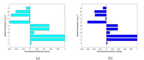
Table 2. The values of parameters used in the simulations.

Parameter	Description	Values	Reference
r	Growth rate of coffee biomass	0.25 ${\mathrm{d}\mathrm{a}\mathrm{y}}^{-1}$	Estimated
k	Carrying capacity	10 ${\mathrm{m}}^{-2}$	Estimated
β	Rate of farmers activity due to awareness	0.28 ${\mathrm{d}\mathrm{a}\mathrm{y}}^{-1}$	Estimated
μ	Natural mortality rate of healthy coffee berries	0.052 ${\mathrm{d}\mathrm{a}\mathrm{y}}^{-1}$	Estimated
σ	Conversion rate from coffee berries to CBB	0.6	[43]
α	Aware farmer growth rate	0.325 ${\mathrm{d}\mathrm{a}\mathrm{y}}^{-1}$	Estimated
γ	Attack rate of female borer on berries	0.535 ${\mathrm{p}\mathrm{e}\mathrm{s}\mathrm{t}}^{-1}{\mathrm{d}\mathrm{a}\mathrm{y}}^{-1}$	Estimated
c	Half saturation rate of healthy coffee berries with CBB	1 ${\mathrm{d}\mathrm{a}\mathrm{y}}^{-1}$	Estimated
d	Natural mortality rate of CBB	1/81 ${\mathrm{d}\mathrm{a}\mathrm{y}}^{-1}$	[31]
e	A rate at which awareness decrease	0.45 ${\mathrm{d}\mathrm{a}\mathrm{y}}^{-1}$	Estimated
δ	Half saturation rate of level awareness with CBB	0.675 ${\mathrm{d}\mathrm{a}\mathrm{y}}^{-1}$	Estimated
θ	Rate awareness from global source	0.02 ${\mathrm{d}\mathrm{a}\mathrm{y}}^{-1}$	Estimated

4. Extension of the model into optimal control

In this section, we extend the proposed model (1(1) $\begin{array}{rl}{\displaystyle \frac{\mathrm{d}B}{\mathrm{d}t}}& =rB(1-{\displaystyle \frac{B}{k}})-{\displaystyle \frac{\gamma BY}{c+B}}-\mu B,\\ {\displaystyle \frac{\mathrm{d}Y}{\mathrm{d}t}}& ={\displaystyle \frac{\sigma \gamma BY}{c+B}}-{\displaystyle \frac{\text{β}AY}{\delta +A}}-\mathrm{d}Y,\\ {\displaystyle \frac{\mathrm{d}A}{\mathrm{d}t}}& =\theta +\alpha Y-eA,\end{array}$(1) ) into the optimal control problem. Hence, we want to advise the concerned the effectiveness of those strategies if they are fulfilled at an optimal level. This helped us to identify the best control strategies that were used to eradicate the pests from the coffee berry population in the specified time.

As one approach, we proposed educating coffee farmers on the CBB life cycle and its reservoir for effective management in combination with the trap. Because after harvest, all the remaining coffee berries that have fallen must be removed as they are a reservoir in which the CBB can live until the next coffee crop is ripe enough to infest. The method is environmentally friendly but labour intensive. The trap also helps to minimize the female borer, but it is useful only when the pest is outside the fruit.

To apply optimal control, we classify those activities into two groups listed below. The first control $u_1$ represents the effort made to reduce the colonizing females by using chemicals, traps, and biological control (Beauveria bassiana), that are applied to the surface of the coffee berries and kill the colonizing females of CBB when they drill an entry hole into the coffee berry. The second control $u_2$ represents the effort made to increase the awareness of farmers through media campaign and education for coffee farmer. The corresponding state system for model (1(1) $\begin{array}{rl}{\displaystyle \frac{\mathrm{d}B}{\mathrm{d}t}}& =rB(1-{\displaystyle \frac{B}{k}})-{\displaystyle \frac{\gamma BY}{c+B}}-\mu B,\\ {\displaystyle \frac{\mathrm{d}Y}{\mathrm{d}t}}& ={\displaystyle \frac{\sigma \gamma BY}{c+B}}-{\displaystyle \frac{\text{β}AY}{\delta +A}}-\mathrm{d}Y,\\ {\displaystyle \frac{\mathrm{d}A}{\mathrm{d}t}}& =\theta +\alpha Y-eA,\end{array}$(1) ) is given by (22) $\{\begin{array}{ll}{\displaystyle \frac{\mathrm{d}B}{\mathrm{d}t}}& =rB(1-{\displaystyle \frac{B}{K}})-{\displaystyle \frac{\gamma (1-u_1)BY}{c+B}}-\mu B,\\ {\displaystyle \frac{\mathrm{d}Y}{\mathrm{d}t}}& ={\displaystyle \frac{(1-u_1)\sigma \gamma BY}{c+B}}-{\displaystyle \frac{\text{β}AY}{\delta +A}}-dY,\\ {\displaystyle \frac{\mathrm{d}A}{\mathrm{d}t}}& =\theta +u_2+\alpha Y-eA,\end{array}$(22) where $B\left(0\right)=B_0>0,Y\left(0\right)=Y_0\ge 0,A\left(0\right)=A_0>0$.

The number of CBB Y and the implementation cost of strategies related to the controls $u_1$ and $u_2$ are considered in cost functional (23(23) $J[u_1,u_2]={\int }_0^T\left(CY\right(t)+\frac{1}{2}\sum _{i=1}^2{M}_i{u}_i^2)\mathrm{d}t\to min,$(23) ). The cost functional can be defined for the minimization problem as (23) $J[u_1,u_2]={\int }_0^T\left(CY\right(t)+\frac{1}{2}\sum _{i=1}^2{M}_i{u}_i^2)\mathrm{d}t\to min,$(23) where constants C, $M_1$ and $M_2$ are positive. The weight constants $M_1$ and $M_2$ are the measure of relative costs of interventions associated with the controls $u_1$ and $u_2$, respectively, and also balance the units of the integrand. Larger values of $M_1$ and $M_2$ tell us the expensiveness of implementation cost. The terms $\frac{1}{2}{M}_1{u}_1$ and $\frac{1}{2}{M}_2{u}_2$ describe the cost associated with the traps, biological control, and awareness campaign, respectively. In the cost function, the term $CY\left(t\right)$ describes the cost related to killing colonizing female borers at the end of the season. The quadratic term in the objective function is taken because the intervention is nonlinear [36,37]. Moreover, the functional $\mathit{J}$ corresponds to the total cost due to CBB infestation and its control strategies.

Further, the integrand function $L(t,B,Y,A,u_1,u_2)=CY\left(t\right)+\frac{1}{2}\sum _{i=1}^2{M}_i{u}_i^2$ measures the current cost at time t. The fixed constant T denotes the terminal treatment time. The set of admissible controls is defined as (24) $V=\left\{u_1\right(\cdot ),u_2(\cdot )\in L^{\mathrm{\infty }}(0,T):0\le u(t)<1,\mathrm{\forall }t\in [0,t\left]\right\}.$(24) Then, we consider the optimal control problem of determining $\left(B^{\ast }\right(\cdot ),Y^{\ast }(\cdot ),A^{\ast }(\cdot \left)\right)$ associated with an admissible control $(u_1^{\ast },u_2^{\ast })\in V$ on the intervention time interval $[0,T]$, subjected to the state control system (22(22) $\{\begin{array}{ll}{\displaystyle \frac{\mathrm{d}B}{\mathrm{d}t}}& =rB(1-{\displaystyle \frac{B}{K}})-{\displaystyle \frac{\gamma (1-u_1)BY}{c+B}}-\mu B,\\ {\displaystyle \frac{\mathrm{d}Y}{\mathrm{d}t}}& ={\displaystyle \frac{(1-u_1)\sigma \gamma BY}{c+B}}-{\displaystyle \frac{\text{β}AY}{\delta +A}}-dY,\\ {\displaystyle \frac{\mathrm{d}A}{\mathrm{d}t}}& =\theta +u_2+\alpha Y-eA,\end{array}$(22) ) in ${\mathbb{R}}^3$ with its initial data and minimizing the cost functional (23(23) $J[u_1,u_2]={\int }_0^T\left(CY\right(t)+\frac{1}{2}\sum _{i=1}^2{M}_i{u}_i^2)\mathrm{d}t\to min,$(23) ). More precisely, the optimal control problem can be defined as (25) $J[u_1^{\ast },u_2^{\ast }]=\underset{V}{min}J\left[u_1\right(\cdot ),u_2(\cdot \left)\right]$(25) satisfying (22(22) $\{\begin{array}{ll}{\displaystyle \frac{\mathrm{d}B}{\mathrm{d}t}}& =rB(1-{\displaystyle \frac{B}{K}})-{\displaystyle \frac{\gamma (1-u_1)BY}{c+B}}-\mu B,\\ {\displaystyle \frac{\mathrm{d}Y}{\mathrm{d}t}}& ={\displaystyle \frac{(1-u_1)\sigma \gamma BY}{c+B}}-{\displaystyle \frac{\text{β}AY}{\delta +A}}-dY,\\ {\displaystyle \frac{\mathrm{d}A}{\mathrm{d}t}}& =\theta +u_2+\alpha Y-eA,\end{array}$(22) ) and its initial data.

4.1. Existence of the optimal control

In this subsection, we prove the existence of optimal control functions which minimize the cost function in the finite intervention period. The following result guarantees the existence of optimal control functions. A detailed and similar analysis of the existence of optimal control can be found in [38,39].

Theorem 4.1

There exists an optimal control $(u_1^{\ast },u_2^{\ast })$ and a corresponding solution vector $(B^{\ast },Y^{\ast },A^{\ast })$ to the state system (22(22) $\{\begin{array}{ll}{\displaystyle \frac{\mathrm{d}B}{\mathrm{d}t}}& =rB(1-{\displaystyle \frac{B}{K}})-{\displaystyle \frac{\gamma (1-u_1)BY}{c+B}}-\mu B,\\ {\displaystyle \frac{\mathrm{d}Y}{\mathrm{d}t}}& ={\displaystyle \frac{(1-u_1)\sigma \gamma BY}{c+B}}-{\displaystyle \frac{\text{β}AY}{\delta +A}}-dY,\\ {\displaystyle \frac{\mathrm{d}A}{\mathrm{d}t}}& =\theta +u_2+\alpha Y-eA,\end{array}$(22) ) that minimize the cost functional $\mathit{J}\mathit{\left(}\mathit{u}\mathit{\right)}$ of (23(23) $J[u_1,u_2]={\int }_0^T\left(CY\right(t)+\frac{1}{2}\sum _{i=1}^2{M}_i{u}_i^2)\mathrm{d}t\to min,$(23) ) over the set of admissible control V.

Proof.

All the state variables involved in the model are continuously differentiable. Therefore, we need to verify the following four conditions given in [38].

1. The set of all solution to state system (22(22) $\{\begin{array}{ll}{\displaystyle \frac{\mathrm{d}B}{\mathrm{d}t}}& =rB(1-{\displaystyle \frac{B}{K}})-{\displaystyle \frac{\gamma (1-u_1)BY}{c+B}}-\mu B,\\ {\displaystyle \frac{\mathrm{d}Y}{\mathrm{d}t}}& ={\displaystyle \frac{(1-u_1)\sigma \gamma BY}{c+B}}-{\displaystyle \frac{\text{β}AY}{\delta +A}}-dY,\\ {\displaystyle \frac{\mathrm{d}A}{\mathrm{d}t}}& =\theta +u_2+\alpha Y-eA,\end{array}$(22) ) with corresponding control functions in (24(24) $V=\left\{u_1\right(\cdot ),u_2(\cdot )\in L^{\mathrm{\infty }}(0,T):0\le u(t)<1,\mathrm{\forall }t\in [0,t\left]\right\}.$(24) ) is non-empty;

2. The control set is convex and closed;

3. The right-hand side of the state system (22(22) $\{\begin{array}{ll}{\displaystyle \frac{\mathrm{d}B}{\mathrm{d}t}}& =rB(1-{\displaystyle \frac{B}{K}})-{\displaystyle \frac{\gamma (1-u_1)BY}{c+B}}-\mu B,\\ {\displaystyle \frac{\mathrm{d}Y}{\mathrm{d}t}}& ={\displaystyle \frac{(1-u_1)\sigma \gamma BY}{c+B}}-{\displaystyle \frac{\text{β}AY}{\delta +A}}-dY,\\ {\displaystyle \frac{\mathrm{d}A}{\mathrm{d}t}}& =\theta +u_2+\alpha Y-eA,\end{array}$(22) ) is bounded by a linear function in the state and control variable;

4. The integrand L of (23(23) $J[u_1,u_2]={\int }_0^T\left(CY\right(t)+\frac{1}{2}\sum _{i=1}^2{M}_i{u}_i^2)\mathrm{d}t\to min,$(23) ) is convex on V and $L(t,B,Y,A,u)\ge g\left(u\right)$, where g is continuous and $||u|{|}^{-1}g\left(u\right)⟶+\mathrm{\infty }$ as $||u||⟶\mathrm{\infty }$.

The existence of the solution of the system (22(22) $\{\begin{array}{ll}{\displaystyle \frac{\mathrm{d}B}{\mathrm{d}t}}& =rB(1-{\displaystyle \frac{B}{K}})-{\displaystyle \frac{\gamma (1-u_1)BY}{c+B}}-\mu B,\\ {\displaystyle \frac{\mathrm{d}Y}{\mathrm{d}t}}& ={\displaystyle \frac{(1-u_1)\sigma \gamma BY}{c+B}}-{\displaystyle \frac{\text{β}AY}{\delta +A}}-dY,\\ {\displaystyle \frac{\mathrm{d}A}{\mathrm{d}t}}& =\theta +u_2+\alpha Y-eA,\end{array}$(22) ) is obtained in using result from [40], (Theorem 9.2.1), since state system (22(22) $\{\begin{array}{ll}{\displaystyle \frac{\mathrm{d}B}{\mathrm{d}t}}& =rB(1-{\displaystyle \frac{B}{K}})-{\displaystyle \frac{\gamma (1-u_1)BY}{c+B}}-\mu B,\\ {\displaystyle \frac{\mathrm{d}Y}{\mathrm{d}t}}& ={\displaystyle \frac{(1-u_1)\sigma \gamma BY}{c+B}}-{\displaystyle \frac{\text{β}AY}{\delta +A}}-dY,\\ {\displaystyle \frac{\mathrm{d}A}{\mathrm{d}t}}& =\theta +u_2+\alpha Y-eA,\end{array}$(22) ) has bounded coefficients and any solution is bounded on the finite interval time $[0,T]$, so condition (i) is satisfied. To proof (ii), consider $V=\{u\in \mathbb{R}:||u||\le 1\}.$Let $u_1,u_2\in V$ such that $||u_1||\le 1$ and $||u_2||\le 1$. Then for any $\text{β}\in [0,1]$, $||\text{β}{u}_1+(1-\text{β})u_2||\le \text{β}||u_1||+(1-\text{β})||u_2||\le 1.$This implies that the control set V is convex and closed. The state system (22(22) $\{\begin{array}{ll}{\displaystyle \frac{\mathrm{d}B}{\mathrm{d}t}}& =rB(1-{\displaystyle \frac{B}{K}})-{\displaystyle \frac{\gamma (1-u_1)BY}{c+B}}-\mu B,\\ {\displaystyle \frac{\mathrm{d}Y}{\mathrm{d}t}}& ={\displaystyle \frac{(1-u_1)\sigma \gamma BY}{c+B}}-{\displaystyle \frac{\text{β}AY}{\delta +A}}-dY,\\ {\displaystyle \frac{\mathrm{d}A}{\mathrm{d}t}}& =\theta +u_2+\alpha Y-eA,\end{array}$(22) ) is clearly linear in control variables $u_1$ and $u_2$ with coefficients depending on state variables. With this condition (iii) is satisfied. The integrand of the cost functional (26) $L(t,B,Y,A,u)=CY\left(t\right)+{\displaystyle \frac{1}{2}}\sum _{i=1}^2{M}_i{u}_i^2\ge {\displaystyle \frac{1}{2}}\sum _{i=1}^2{M}_i{u}_i^2$(26) let $\xi =min(\frac{M_1}{2},\frac{M_2}{2})>0$, and define a continuous function $g\left(u\right)=\xi ||u|{|}^2$. Then from Equation (26(26) $L(t,B,Y,A,u)=CY\left(t\right)+{\displaystyle \frac{1}{2}}\sum _{i=1}^2{M}_i{u}_i^2\ge {\displaystyle \frac{1}{2}}\sum _{i=1}^2{M}_i{u}_i^2$(26) ) we have $L(t,B,Y,A,u)\ge g\left(u\right)$. Clearly $||u|{|}^{-1}g\left(u\right)⟶+\mathrm{\infty }$ as $||u||⟶\mathrm{\infty }$. Thus, condition (iv) is achieved. Therefore, the existence of an optimal control pair $(X^{\ast },u^{\ast })$ satisfying Equations (22(22) $\{\begin{array}{ll}{\displaystyle \frac{\mathrm{d}B}{\mathrm{d}t}}& =rB(1-{\displaystyle \frac{B}{K}})-{\displaystyle \frac{\gamma (1-u_1)BY}{c+B}}-\mu B,\\ {\displaystyle \frac{\mathrm{d}Y}{\mathrm{d}t}}& ={\displaystyle \frac{(1-u_1)\sigma \gamma BY}{c+B}}-{\displaystyle \frac{\text{β}AY}{\delta +A}}-dY,\\ {\displaystyle \frac{\mathrm{d}A}{\mathrm{d}t}}& =\theta +u_2+\alpha Y-eA,\end{array}$(22) ) and (25(25) $J[u_1^{\ast },u_2^{\ast }]=\underset{V}{min}J\left[u_1\right(\cdot ),u_2(\cdot \left)\right]$(25) ) is assured by results given in [38].

4.2. Characterization of the optimal control solution

In order to derive the necessary conditions for the optimal control pair, Pontryagin's minimum principle [41] is used. According to the this principle, for $(u_1^{\ast },u_2^{\ast })$ to be optimal with corresponding optimal state $(B^{\ast },Y^{\ast },A^{\ast })$ which minimizes the cost functional (22(22) $\{\begin{array}{ll}{\displaystyle \frac{\mathrm{d}B}{\mathrm{d}t}}& =rB(1-{\displaystyle \frac{B}{K}})-{\displaystyle \frac{\gamma (1-u_1)BY}{c+B}}-\mu B,\\ {\displaystyle \frac{\mathrm{d}Y}{\mathrm{d}t}}& ={\displaystyle \frac{(1-u_1)\sigma \gamma BY}{c+B}}-{\displaystyle \frac{\text{β}AY}{\delta +A}}-dY,\\ {\displaystyle \frac{\mathrm{d}A}{\mathrm{d}t}}& =\theta +u_2+\alpha Y-eA,\end{array}$(22) ) for a fixed final time T, then there exists a non-trivial absolutely continuous mapping $\lambda :[0,T]⟶{\mathbb{R}}^3,\lambda \left(t\right)=\left({\lambda }_1\right(t),{\lambda }_2(t),{\lambda }_3(t\left)\right)$ called the adjoint vector such that

1. the Hamiltonian function is defined as (27) $\mathcal{H}=CY\left(t\right)+{\displaystyle \frac{1}{2}}\sum _{i=1}^2{M}_i{u}_i^2+\sum _{i=1}^3{\lambda }_i{g}_i(t,B,Y,A,u_1,u_2),$(27) where $g_i$ stands for the right hands of the constraints (22(22) $\{\begin{array}{ll}{\displaystyle \frac{\mathrm{d}B}{\mathrm{d}t}}& =rB(1-{\displaystyle \frac{B}{K}})-{\displaystyle \frac{\gamma (1-u_1)BY}{c+B}}-\mu B,\\ {\displaystyle \frac{\mathrm{d}Y}{\mathrm{d}t}}& ={\displaystyle \frac{(1-u_1)\sigma \gamma BY}{c+B}}-{\displaystyle \frac{\text{β}AY}{\delta +A}}-dY,\\ {\displaystyle \frac{\mathrm{d}A}{\mathrm{d}t}}& =\theta +u_2+\alpha Y-eA,\end{array}$(22) ) for i = 1, 2, 3.

2. The control system (28) $B^{\prime }={\displaystyle \frac{\mathrm{\partial }\mathcal{H}}{\mathrm{\partial }{\lambda }_1}},Y^{\prime }={\displaystyle \frac{\mathrm{\partial }\mathcal{H}}{\mathrm{\partial }{\lambda }_2}},A^{\prime }={\displaystyle \frac{\mathrm{\partial }\mathcal{H}}{\mathrm{\partial }{\lambda }_3}}.$(28)

3. The adjoint system (29) ${\lambda }_1^{\prime }=-{\displaystyle \frac{\mathrm{\partial }\mathcal{H}}{\mathrm{\partial }B}},{\lambda }_2^{\prime }=-{\displaystyle \frac{\mathrm{\partial }\mathcal{H}}{\mathrm{\partial }Y}},{\lambda }_3^{\prime }=-{\displaystyle \frac{\mathrm{\partial }\mathcal{H}}{\mathrm{\partial }A}}.$(29)

4. The optimality condition (30) $\mathcal{H}\left(B^{\ast }\right(t),Y^{\ast }(t),A^{\ast }(t),u^{\ast }(t),{\lambda }^{\ast }(t\left)\right)=\underset{u\in V}{min}\mathcal{H}\left(B\right(t),Y(t),A(t),u(t),\lambda (t\left)\right)$(30) holds for almost all $t\in [0,T]$

5. Moreover, the transversality condition (31) ${\lambda }_1\left(T\right)=0,{\lambda }_2\left(T\right)=0,{\lambda }_2\left(T\right)=0,\text{also holds true.}$(31)

Theorem 4.2

There exists an optimal solution $\left(B^{\ast }\right(t),Y^{\ast }(t),A^{\ast }(t\left)\right)$ and corresponding optimal control $u^{\ast }=(u_1^{\ast },u_2^{\ast })$ that minimize $J(u_1,u_2)$ over the set of admissible control Ω. Moreover, there exists an adjoint function ${\lambda }_i^{\ast }\left(t\right),i=1,2,3$ such that (32) $\{\begin{array}{l}{\lambda }_1^{\prime }=({\lambda }_1-\sigma {\lambda }_2){\displaystyle \frac{c(1-u_1)\gamma Y}{(c+B{)}^2}}+{\lambda }_1({\displaystyle \frac{2rB}{K}}-r+\mu ),\\ {\lambda }_2^{\prime }=-C+({\lambda }_1-\sigma {\lambda }_2){\displaystyle \frac{(1-u_1)\gamma B}{(c+B)}}+{\lambda }_2({\displaystyle \frac{\text{β}A}{\delta +A}}+d)-\alpha {\lambda }_3,\\ {\lambda }_3^{\prime }={\lambda }_2{\displaystyle \frac{\delta \text{β}Y}{(\delta +A{)}^2}}+e{\lambda }_3,\end{array}$(32) with transversality conditions ${\lambda }_i\left(T\right)=0,i=1,2,3$.

Furthermore, the following properties holds: (33) $\begin{array}{rl}{u}_1^{\ast }& =min\{max\{0,{\displaystyle \frac{\gamma BY}{M_1(c+B)}}(\sigma {\lambda }_2-{\lambda }_1\left)\right\},1\},\\ u_2^{\ast }& =min\{max\{0,-{\displaystyle \frac{{\lambda }_3}{M_2}}\},1\},\end{array}$(33) where ${\lambda }_3\le 0$.

Proof.

The Hamiltonian function associated with the system is defined as follows: $\begin{array}{rl}\mathcal{H}(t,B,Y,A,u_1,u_2)& =CY\left(t\right)+{\displaystyle \frac{1}{2}}{M}_1{u}_1^2+{\displaystyle \frac{1}{2}}{M}_2{u}_2^2\\ & +{\lambda }_1\{rB(1-{\displaystyle \frac{B}{K}})-{\displaystyle \frac{(1-u_1)\gamma BY}{c+B}}-\mu B\}\\ & +{\lambda }_2\{{\displaystyle \frac{(1-u_1)\sigma \gamma BY}{c+B}}-{\displaystyle \frac{\text{β}AY}{\delta +A}}-\mathrm{d}Y\}\\ & +{\lambda }_3\{\theta +u_2+\alpha Y-eA\}.\end{array}$The adjoint system can be obtained as $\begin{array}{r}\{\begin{array}{l}{\displaystyle \frac{\mathrm{d}{\lambda }_1}{\mathrm{d}t}}=-{\displaystyle \frac{\mathrm{\partial }H}{\mathrm{\partial }B}}=({\lambda }_1-\sigma {\lambda }_2){\displaystyle \frac{c(1-u_1)\gamma Y}{(c+B{)}^2}}+{\lambda }_1({\displaystyle \frac{2rB}{K}}+\mu -r),\\ {\displaystyle \frac{\mathrm{d}{\lambda }_2}{\mathrm{d}t}}=-{\displaystyle \frac{\mathrm{\partial }H}{\mathrm{\partial }Y}}=-C+({\lambda }_1-\sigma {\lambda }_2){\displaystyle \frac{(1-u_1)\gamma B}{(c+B)}}+{\lambda }_2({\displaystyle \frac{\text{β}A}{\delta +A}}+d)-\alpha {\lambda }_3,\\ {\displaystyle \frac{\mathrm{d}{\lambda }_3}{\mathrm{d}t}}=-{\displaystyle \frac{\mathrm{\partial }H}{\mathrm{\partial }A}}={\lambda }_2{\displaystyle \frac{\delta \text{β}Y}{(\delta +A{)}^2}}+e{\lambda }_3.\end{array}\end{array}$The state variables are not assigned at the final time T. Hence, from [37], the transversality conditions (or boundary conditions) become ${\lambda }_i\left(T\right)=0,$ for i = 1, 2, 3. By the optimality condition, we have: ${\displaystyle \frac{\mathrm{\partial }\mathcal{H}}{\mathrm{\partial }{u}_i}}=0\mathrm{f}\mathrm{o}\mathrm{r}i=1,2.$That is,

1. ${\displaystyle \frac{\mathrm{\partial }\mathcal{H}}{\mathrm{\partial }{u}_1}}=M_1{u}_1+{\lambda }_1{\displaystyle \frac{\gamma BY}{c+B}}-{\lambda }_2{\displaystyle \frac{\gamma \sigma BY}{c+B}}=0$ ⇔$u_1^{\ast }\left(t\right)=(\sigma {\lambda }_2-{\lambda }_1){\displaystyle \frac{\gamma BY}{M_1(c+B)}}$ at $u_1\left(t\right)=u_1^{\ast }\left(t\right)$.

2. ${\displaystyle \frac{\mathrm{\partial }\mathcal{H}}{\mathrm{\partial }{u}_2}}=M_2{u}_2+{\lambda }_3=0$ ⇔$u_2^{\ast }\left(t\right)=-{\displaystyle \frac{{\lambda }_3}{M_2}}$ at $u_2\left(t\right)=u_2^{\ast }\left(t\right)$.

From boundedness on $u_1^{\ast }\left(t\right)$ and minimality condition, we have: $u_1^{\ast }\left(t\right)=\{\begin{array}{ll}0& \mathrm{i}\mathrm{f}{\displaystyle \frac{\mathrm{\partial }\mathcal{H}}{\mathrm{\partial }{u}_1}}>0,\\ (\sigma {\lambda }_2-{\lambda }_1){\displaystyle \frac{\gamma BY}{M_1(c+B)}}& \mathrm{i}\mathrm{f}{\displaystyle \frac{\mathrm{\partial }\mathcal{H}}{\mathrm{\partial }{u}_1}}=0,\\ 0.95& \mathrm{i}\mathrm{f}{\displaystyle \frac{\mathrm{\partial }\mathcal{H}}{\mathrm{\partial }{u}_1}}<0.\end{array}$Here also from boundedness on $u_2^{\ast }\left(t\right)$ and the minimality condition, we have: $u_2^{\ast }\left(t\right)=\{\begin{array}{ll}0& \mathrm{i}\mathrm{f}{\displaystyle \frac{\mathrm{\partial }\mathcal{H}}{\mathrm{\partial }{u}_1}}>0,\\ -{\displaystyle \frac{{\lambda }_3}{M_2}}& \mathrm{i}\mathrm{f}{\displaystyle \frac{\mathrm{\partial }\mathcal{H}}{\mathrm{\partial }{u}_1}}=0,\\ 1& \mathrm{i}\mathrm{f}{\displaystyle \frac{\mathrm{\partial }\mathcal{H}}{\mathrm{\partial }{u}_1}}<0.\end{array}$In compact notation: $\begin{array}{rl}{u}_1^{\ast }& =min\{max\{0,{\displaystyle \frac{\gamma BY}{M_1(c+B)}}(\sigma {\lambda }_2-{\lambda }_1\left)\right\},1\},\\ u_2^{\ast }& =min\{max\{0,-{\displaystyle \frac{{\lambda }_3}{M_2}}\},1\}.\end{array}$

5. Numerical simulations

In this section, we provide numerical simulations obtained from the application of our analytical results, as given in previous sections. For this purpose, we use the forward-backward sweep method [42]. In order to find numerical solutions of the optimality system, first the state system (22(22) $\{\begin{array}{ll}{\displaystyle \frac{\mathrm{d}B}{\mathrm{d}t}}& =rB(1-{\displaystyle \frac{B}{K}})-{\displaystyle \frac{\gamma (1-u_1)BY}{c+B}}-\mu B,\\ {\displaystyle \frac{\mathrm{d}Y}{\mathrm{d}t}}& ={\displaystyle \frac{(1-u_1)\sigma \gamma BY}{c+B}}-{\displaystyle \frac{\text{β}AY}{\delta +A}}-dY,\\ {\displaystyle \frac{\mathrm{d}A}{\mathrm{d}t}}& =\theta +u_2+\alpha Y-eA,\end{array}$(22) ) is computed forward with the given initial condition and controls initial guess in time by using a Runge–Kutta method of fourth order. Next, the adjoint system (32(32) $\{\begin{array}{l}{\lambda }_1^{\prime }=({\lambda }_1-\sigma {\lambda }_2){\displaystyle \frac{c(1-u_1)\gamma Y}{(c+B{)}^2}}+{\lambda }_1({\displaystyle \frac{2rB}{K}}-r+\mu ),\\ {\lambda }_2^{\prime }=-C+({\lambda }_1-\sigma {\lambda }_2){\displaystyle \frac{(1-u_1)\gamma B}{(c+B)}}+{\lambda }_2({\displaystyle \frac{\text{β}A}{\delta +A}}+d)-\alpha {\lambda }_3,\\ {\lambda }_3^{\prime }={\lambda }_2{\displaystyle \frac{\delta \text{β}Y}{(\delta +A{)}^2}}+e{\lambda }_3,\end{array}$(32) ) is computed backward with the transversality condition in time by using the Runge–Kutta algorithm of fourth order. Each control variable value is modified by averaging the new value and old value arising from the characteristic control (33(33) $\begin{array}{rl}{u}_1^{\ast }& =min\{max\{0,{\displaystyle \frac{\gamma BY}{M_1(c+B)}}(\sigma {\lambda }_2-{\lambda }_1\left)\right\},1\},\\ u_2^{\ast }& =min\{max\{0,-{\displaystyle \frac{{\lambda }_3}{M_2}}\},1\},\end{array}$(33) ). This steps continues many times up to successive iterations are close enough to each other.

To perform the simulation, a set of meaningful values are assigned to the model parameters. These values are either taken from the literature or assumed. Accordingly, parameter values are given in Table 2, and with initial data: $B\left(0\right)=0.02,Y\left(0\right)=0.03,$ and $A\left(0\right)=0.01$. To achieve optimal control strategies, the weight constants of the objective function are assumed: $C=2,M_1=M_2=1$ and the adjoint system with terminal condition: $\lambda \left(T\right)=0;i=1,2,3$ for the implementation time $t_f=45$ months.

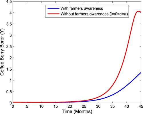
We begin by simulating system (1) without controls. Figure 2(a,b) shows that CBB decreases with aware farmer growth rate and awareness rate increase. From Figure 3, we observe that the number of CBB decreases in the presence.

Figure 2. Impact of aware farmer growth rate and awareness rate on the CBB population.

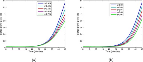
Figure 3. Impact of farmers' awareness and without farmers' awareness on the CBB population.

In Figure 4, the behavioural patterns of the densities of coffee berry biomass, CBB, and aware farmers are presented. All the system populations oscillate initially and finally become asymptotically stable and converge to the endemic state value. Here, it is to be noted that all conditions of Theorem 4 are satisfied and thus the endemic equilibrium $E^{\ast }$ is stable. In the next subsections, we comparatively analyse the impact of control strategies on the infestation of CBB under different scenarios:

• Strategy A: Applying traps or biological control ($u_1$).

• Strategy B: Using farmers awareness ($u_2$).

• Strategy C: Using all controls ($u_1$ and $u_2$).

From Figure 5 the number of healthy coffee berries at the end of the period is increased, but it remains below its value in the pest-free case ($\gamma =0$). More precisely, the number of healthy coffee berry at the end of the period is increased with different control strategies. Clearly, Figure 6 shows that the number of CBB dramatically dropped to zero with different control strategies . Also, optimal control application is time saving and cost-effective. This implies that optimized traps, biological and farmers awareness control reduce the burden of CBB infestation. In Figure 7, farmers awareness decreased with control and will increase without control after reaching the peak of the curve. This is because of fading of memory. In this figure, there is a significant increase and after reaching maximum peak decreases at some period in the number of aware farmers because of fading of memory. Thus, the best choice is to apply both controls all together to eradicate CBB from coffee berry population. The corresponding control profile for control strategies is shown in Figure 8.

Figure 4. Stability behaviour of the endemic state for the system (1(1) $\begin{array}{rl}{\displaystyle \frac{\mathrm{d}B}{\mathrm{d}t}}& =rB(1-{\displaystyle \frac{B}{k}})-{\displaystyle \frac{\gamma BY}{c+B}}-\mu B,\\ {\displaystyle \frac{\mathrm{d}Y}{\mathrm{d}t}}& ={\displaystyle \frac{\sigma \gamma BY}{c+B}}-{\displaystyle \frac{\text{β}AY}{\delta +A}}-\mathrm{d}Y,\\ {\displaystyle \frac{\mathrm{d}A}{\mathrm{d}t}}& =\theta +\alpha Y-eA,\end{array}$(1) ) when $u_1=0$ and $u_2=0$.

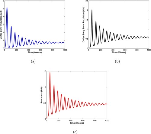
Figure 5. The plot shows the effect of control on healthy coffee berries.

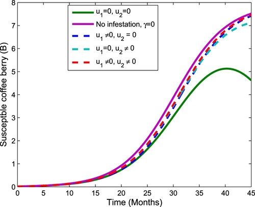
Figure 6. The plot shows the effect of control on coffee berry borer.

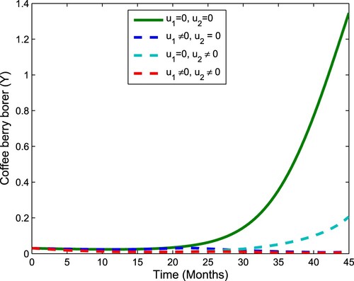
Figure 7. The plot shows the effect of control on farmer aware.

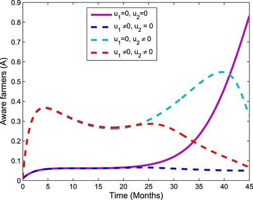
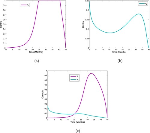
Figure 8. Profile of control functions. (a) Profile of control function $u_1$ when $u_2=0$. (b) Profile of control function $u_2$ when $u_1=0$. (c) Profile of control functions $u_1$ and $u_2$.

6. Cost-effectiveness analysis

In this section, we study cost-effectiveness for three different control strategies. To obtain this, we follow the method applied in [44]. It depends on computing the incremental cost-effectiveness ratio (ICER) and given by $\mathrm{I}\mathrm{C}\mathrm{E}\mathrm{R}=\frac{\text{Difference of costs between two strategies}}{\text{Difference of the total number of their CBB averted}}.$That is, the ICER of strategy A, strategy B, and strategy C is given as (34) $ICER={\int }_0^{45}Y\left(t\right)\mathrm{d}t-{\int }_0^{45}{Y}^{\ast }\left(t\right)\mathrm{d}t,$(34) where $Y\left(t\right)$ is a CBB without control and $Y^{\ast }\left(t\right)$ is a CBB with control. Each control strategy is compared with the next less effective alternative strategies. The total control cost $C\left(u\right)$ is given by (35) $C\left(u\right)=\stackrel{min}{(u_1,u_2)}{\int }_0^{45}({\displaystyle \frac{1}{2}}{b}_1{u}_1^2+{\displaystyle \frac{1}{2}}{b}_2{u}_2^2)\mathrm{d}t.$(35) The functions $0.5b_1{u}_1^2$ and $0.5b_2{u}_2^2$ represent the cost weights associated with control $u_1$ and $u_2$ measure, respectively. The numerical output for the three control strategies are rated incrementally in the form of CBB averted as shown in Table 3.

Table 3. Total coffee berry borer averted and control costs.

Strategy	Description	Coffee berry borer averted	Control costs ($)	ICER
B	Farmers awareness	8.4755	3.5162	0.4149
A	Traps or biological	9.2592	11.2892	9.9183
C	Both controls	9.6990	5.8934	−12.2688

We calculate the ICER for strategy A, strategy B, and strategy C which are given in Table 3 and then compare their results as follows: $\begin{array}{rl}ICER\left(B\right)& ={\displaystyle \frac{3.5162-0}{8.4755-0}}=0.4149,\\ ICER\left(A\right)& ={\displaystyle \frac{11.2892-3.5162}{9.2592-8.4755}}=9.9183,\\ ICER\left(C\right)& ={\displaystyle \frac{5.8934-11.2892}{9.6990-9.2592}}=-\mathrm{12.2688.}\end{array}$The comparison between strategy B and strategy A showed a cost saving of 0.4149 for strategy B over strategy A. This shows that strategy A is more expensive and less effective compared to strategy B. Thus, strategy A is excluded and we continue to compare the ICER for strategy B over strategy C from Table 4 as follows.

Comparing strategy B and strategy C, we observe that ICER (B) is greater than ICER (C). Since strategy B consumes more resources, it has to be excluded from the set of alternatives. This value shows that strategy C is the cheapest. As a result, strategy C is the most cost-effective among the control strategies for the control of coffee berry borer.

7. Conclusions

In this study, we have developed a mathematical model which describes the infestation dynamic of CBB with farmer awareness and optimal control using a system of nonlinear ordinary differential equations. The qualitative analysis reveals that CBB-free equilibrium point is both locally and globally stable for ${\mathcal{R}}_0<1$. If the impact of awareness campaigns increases, the density of crop increases. On the other hand, EEP is both locally and globally stable if ${\mathcal{R}}_0>1$. Sensitivity analyses of the model have been studied and determine a parameter that plays a greater role in the infestation dynamics of CBB. We have used two controls: $\left(u_1\right)$ (traps and biological control) and $\left(u_2\right)$ (awareness of farmers). The Hamiltonian, the adjoint variables, the characterization of the controls, and the optimality system of our model were derived and analysed using Pontryagin's minimum principle. We performed numerical simulations on the optimality system considering integrated strategies, as on seasonal coffee infestation by CBB has used. The numerical results clearly indicate that each integrated management strategy has the power to combat the pest. Therefore, the results of this study show that optimal control is sufficient to decrease pests from the coffee berry population with lowered cost at the end of the forty fifth month.

Table 4. Total coffee berry borer averted, control costs and ICER.

Strategy	Description	CBB averted	Control costs ($)	ICER
B	Farmers awareness	8.4755	3.5162	0.4149
C	Both controls	9.6990	5.8934	−12.2688

Acknowledgments

The authors thank Adama Science and Technology University for its hospitality and support during this work.

Disclosure statement

No potential conflict of interest was reported by the author(s).

References

- Coffee FSP. Food and agriculture organization of the United Nations. 2015.
- Vega F. Coffee berry borer Hypothenemus hampei (ferrari) (coleoptera: scolytidae). Encycl Entomol. 2004;1:575–576.
- Murphy ST, Moore D. Biological control of the coffee berry borer, Hypothenemus hampei, (ferrari) (coleoptera: scolytida): previous programmes and possibilities for the future. Biocontrol News Info. 1990;11:107–117.
- Fuad A. Studies on the diversity of insect pests in wild and cultivated coffee plantations in and around Jimma, southwest Ethiopia. Int J Biodivers Conserv. 2010;8(10):233–243.
- Vega FE, Mercadier G, Dowd PF, et al. Fungi associated with the coffee berry borer Hypothenemus hampei (ferrari)(coleoptera: scolytidae). Colloq Sci Int Cafe (C.R.). 1999;18:229–238.
- Burbano E, Wright M, Bright DE, et al. New record for the coffee berry borer, Hypothenemus hampei, in Hawaii. J Insect Sci. 2011;11(117):1–3. Available online: insectscience.org/11.117.
- Chaves B, Riley J. Determination of factors influencing integrated pest management adoption in coffee berry borer in Colombian farms. Agric Ecosyst Environ. 2001;87(2):159–177.
- Damon A. A review of the biology and control of the coffee berry borer, Hypothenemus hampei (coleoptera: scolytidae). Bull Entomol Res. 2000;90(6):453–465.
- Aristizabal LF, Bustillo AE, Arthurs SP. Integrated pest management of coffee berry borer: strategies from Latin America that could be useful for coffee farmers in Hawaii. Insects. 2016;7(1):6.
- Mercanta Coffee Hunter. Coffee berry borer: What is and what damages it causes; 2016.
- Khan GA, Muhammad S, Khan MA. Information regarding agronomic practices and plant protection measures obtained by the farmers through electronic me dia. J Anim Plant Sci. 2013;23(2):647–650.
- Marcano M, Bose A, Bayman P. A one dimensional map to study multiseasonal coffee infestation by the coffee berry borer. Math Biosci. 2021;333:Article ID 108530.
- Horub KE, Julius T. A mathematical model for the vector transmission and control of banana xanthomonas wilt. J Math Res. 2017;9(4):101–113.
- Jeger MJ, Holt J, Van Den Bosch F, et al. Epidemiology of insect-transmitted plant viruses: modelling disease dynamics and control interventions. Physiol Entomol. 2004;29(3):291–304.
- Fitri IR, Hanum F, Kusnanto A, et al. Optimal pest control strategies with cost-effectiveness analysis. Sci World J. 2021;2021:Article ID 6630193. doi:10.1155/2021/6630193.
- Marcano M, Bose A, Bayman P. A one-dimensional map to study multi-seasonal coffee infestation by the coffee berry borer. Math Biosci. 2021;333:Article ID 108530.
- Rodríguez D, Cure JR, Cotes JM, et al. A coffee agroecosystem model: I. Growth and development of the coffee plant. Ecol Modell. 2011;222(19):3626–3639.
- Rodríguez D, Cure JR, Gutierrez AP, et al. A coffee agroecosystem model: II. Dynamics of coffee berry borer. Ecol Modell. 2013;248:203–214.
- Rodríguez D, Cure JR, Gutierrez AP, et al. A coffee agroecosystem model: III. Parasitoids of the coffee berry borer (Hypothenemus hampei). Ecol Modell. 2017;363:96–110.
- Melese AS, Makinde OD, Obsu LL. Modelling and analysis of pathogens impact on the plant disease transmission with optimal control. J Appl Nonlinear Dyn. 2022;11(3):499–521.
- Melese AS, Makinde OD, Obsu LL. Mathematical modelling and analysis of coffee berry disease dynamics on a coffee farm. Math Biosci Eng. 2022;19(7):7349–7373.
- Fotsa D, Houpa E, Bekolle D, et al. Mathematical modelling and optimal control of anthracnose. arXiv preprint arXiv:1307.1754. 2013.
- Mbogne DJF, Thron C. Optimal control of anthracnose using mixed strategies. Math Biosci. 2015;269:186–198.
- Abraha T, Al Basir F, Obsu LL, et al. Pest control using farming awareness: impact of time delays and optimal use of biopesticides. Chaos Solit Fractals. 2021;146(2021):Article ID 110869.
- Al BasIr F, Banerjee A, Ray S. Role of farming awareness in crop pest management – a mathematical model. J Theoret Biol. 2019;461:59–67.
- Khan GA, Muhammad S, Khan MA. Information regarding agronomic practices and plant protection measures obtained by the farmers through electronic media. J Anim Plant Sci. 2013;23(2):647–650.
- Cunniffe NJ, Gilligan CA. Invasion, persistence and control in epidemic models for plant pathogens: the effect of host demography. J R Soc Interface. 2010;7(44):439–451.
- Abawari MA. A mathematical model for coffee berry borer management in coffee farm with optimal control [dissertation]. Adama (Ethiopia): ASTU; 2021.
- Chowdhurya J, Basir FA, Takeuchic Y, et al. A mathematical model for pest management in Jatropha curcas with integrated pesticides – an optimal control approach. Ecol Complex. 2019;37:24–31.
- Johnson MA, Ruiz-Diaz CP, Manoukis NC, et al. Coffee berry borer (Hypothenemus hampei), a global pest of coffee: perspectives from historical and recent invasions, and future priorities. Insects. 2020;11(12):882.
- Fotso Fotso Y, Grognard F, Tsanou B, et al. Modelling and control of coffee berry borer infestation. HAL Id: hal-01871508. 2018.
- Driessche P, Watmough J. Reproduction numbers and subthreshold endemic equilibria for compartment models of disease transmission. Math Biosci. 2002;180(1-2):29–48.
- Mojeeb A, Osman E, Isaac AK. Simple mathematical model for malaria transmission. J Adv Math Comp Sci. 2017;25:1–24.
- LaSalle JP. The stability of dynamical systems. Philadelphia (PA): Society for Industrial and Applied Mathematics; 1976.
- Chitnis N, Cushing JM, Hyman JM. Bifurcation analysis of a mathematical model for malaria transmission. SIAM J Appl Math. 2006;67(1):24–45.
- Chowdhury J, Al Basir F, Takeuchi Y, et al. A mathematical model for pest management in Jatropha curcas with integrated pestcides – an optimal control approach. Ecol Complex. 2019;37:24–31.
- Al Basir F, Ray S. Impact of farming awareness based roguing, insecticide spraying and optimal control on the dynamics of mosaic disease. Ric Di Mat. 2020;69(1):1–11.
- Fleming WH, Rishel RW. Deterministic and stochastic optimal control. Vol. 1. New York: Springer Science & Business Media; 2012.
- Kumar S, Takeuchi Y. Optimal control of infectious disease: information-induced vaccination and limited treatment. Phys A: Stat Mech Appl. 2020;542:123196.
- Lukes DL. Differential equations: classical to controlled. 1982.
- Pontryagin LS. Mathematical theory of optimal processes. London (UK): Routledge; 2018.
- Lenhart S, Workman JT. Optimal control applied to biological models. London (UK): CRC Press; 2007.
- Abraha T, Al Basir F, Obsu LL, et al. Pest control using farming awareness: impact of time delays and optimal use of biopesticides. Chaos Solit Fractals. 2021;146:110869.
- Alemneh HT, Makinde OD, Theuri DM. Optimal control model and cost effectiveness analysis of maize streak virus pathogen interaction with pest invasion in maize plant. Egypt J Basic Appl Sci. 2020;7(1):180–193.