Artificial neural network for solving the nonlinear singular fractional differential equations

Abstract

This paper proposes an artificial neural network (ANN) architecture for solving nonlinear fractional differential equations. The proposed ANN algorithm is based on a truncated power series expansion to substitute the unknown functions in the equations in this approach. Then, a set of algebraic equations is resolved using the ANN technique in an iterative minimization process. Finally, numerical examples are provided to demonstrate the usefulness of the ANN architectures. The results verify that the suggested ANN architecture achieves high accuracy and good stability.

Keywords:

• MLP neural network
• nonlinear fractional differential equation
• unsupervised learning
• approximate solutions

Mathematics Subject Classifications:

• 41A10
• 68T07
• 34K37

1. Introduction

The study of applications of arbitrary-order integrals, differentials, and mathematical characteristics is done in fractional calculus. The fractional calculus operator is highly appropriate for necessarily suitable with genetic traits and storage. Recently, this topic has gained popularity among scientists due to its extensive use in several branches of engineering, research [1–6] and many others. The investigation of fractional differential equations (FDEs) has received significant interest and is now an evolving research topic. In [7], the authors investigated the stability analysis and system characteristics of the Caputo sense fractional model of Nipah virus transmission. In [8], the human liver is mathematically modeled using the Caputo-Fabrizio fractional derivative and numerically analyzed with real clinical data. In [9], a regularized fractional derivative Ψ -Hilfer is analyzed, as well as various applications. The study of [10] examines a mathematical model for a real-world cholera outbreak employing the Caputo fractional derivative. In [11], within the framework of fractional calculus, the authors examined the dynamics of the motion of an accelerating mass-spring system. Fractional-order differential equations typically have difficulty solving analytically, and their approximations and numerical solutions are of growing interest to researchers. Therefore, it is critical to creating some solid and effective strategies for managing FDEs.

Compared to conventional numerical techniques, ANN approximation computing appears to be less sensitive to the spatial dimension. ANN offers a flexible mesh; however, it does not need to directly deal with the mesh; instead, it simply needs to find a solution to the optimization task. Based on these characteristics and benefits, Lagaris et al. [12] invented the network technique for the Differential Equations problem early on. In [13], a second-order perturbed delay Lane-Emden model originating in astrophysics is solved using a neural swarm technique based on ANN. In [14], the classic Lane-Emden model is used to create a singular third-order perturbed delay differential model with its two kinds, and it is solved using the ANN procedure. In [15], a neuro-evolutionary method based on ANN is given for addressing a class of unique singly disturbed boundary value problems. The authors of [16] have offered an analysis of the fractional singular perturbed model based on fractional order derivatives and perturbation terms. In [17], the authors present a computationally intelligent method to solve the third type of nonlinear pantograph Lane-Emden differential problem. In [18], a singular multi-pantograph delay differential equation has been solved using the ANN technique with optimization of the genetic algorithm. In [19], a Python library named NeuroDiffEq is proposed to solve differential equations with ANN. In [20], Wu et al. developed a wavelet neural network (WNN) with the structure $1\times n\times 1$ to solve the fractional differential equations and gave the conditions for convergence. In [21], Gao et al. proposed a triangle neural network to solve Caputo-type fractional differential equations. Earlier this decade, the use of ANNs to solve FDEs has attracted a lot of attention from various scholars and specialists [22–25].

Due to their numerous benefits, ANNs are gaining importance. For example, it provides error detection and resilience for any quantitative or qualitative characteristics recorded in each neuron in the network with adjacent allocation and can perfectly simulate any extremely nonlinear connection. They may use parallel distributed processing techniques, which can accelerate the completion of large-scale activities, and they can recognize and adapt to new or ambiguous systems. Additionally, the power series approach can be utilized to solve challenging mathematical problems, can offer a series polynomial as a resolution function, and can be used to compute the coefficient. Various real-world problems have been modeled in FDEs, as mentioned above. Simple FDEs can be solved analytically method. However, solving complex FDEs are challenging for analytical and numerical methods. In this paper, we produce an approximation solution of the FDEs,a specific fractional-order Lane-Emden equation, and a nonlinear higher fractional-order differential equation. For this purpose, we integrate the ANN structure with the truncated power series approach in an iterative minimization process. Here, we employ Caputo's definitions for fractional differentials.

The rest of the paper is organized as follows; Section 2 presents the framework, including a brief overview of the problem and the definitions and notation of fractional calculus. Section 3 describes the implementation of the ANN algorithm. Section 4 uses a suitable truncated series expansion to express the answer. The problem becomes a minimization problem by applying the mean squared error function. Also, numerical examples are provided to demonstrate the usefulness of the suggested approach. Section 4 concludes the study and gives the future direction of the approach.

2. Preliminaries

This section initially provides some basic notation and concepts for fractional calculus.

Definition 2.1

Let $h\left(x\right)$ be the differential function on $L_2[a,b]$. The fractional integral of $h\left(x\right)$ is defined as (1) ${}_0{\mathcal{I}}_x^{\nu }h\left(x\right)=\frac{1}{\mathrm{\Gamma }\left(\nu \right)}{\int }_0^x\frac{h\left(\eta \right)}{(x-\eta {)}^{1-\nu }}\mathrm{d}\eta ,\nu >0,$(1) where $\mathrm{\Gamma }(\cdot )$ represents the Gamma function.

Definition 2.2

Let $h\left(x\right)$ be the differential function on $L_2[a,b]$, then the Caputo fractional derivatives of $h\left(x\right)$ are defined by (2) $\begin{array}{rl}{}_a^C{\mathcal{D}}_x^{\nu }h\left(x\right)& =\frac{1}{\mathrm{\Gamma }(n-\nu )}{\int }_a^x\frac{h^n\left(\eta \right)}{(x-\eta {)}^{\nu -n+1}}\mathrm{d}\eta ,\end{array}$(2) (3) $\begin{array}{rl}{}_x^C{\mathcal{D}}_b^{\nu }h\left(x\right)& =\frac{(-1{)}^n}{\mathrm{\Gamma }(n-\nu )}{\int }_x^b\frac{h^n\left(\eta \right)}{(\eta -x{)}^{\nu -n+1}}\mathrm{d}\eta ,\end{array}$(3) where ν is a fractional number, n is a natural number of N, and $\mathrm{\Gamma }(\cdot )$ represents the gamma function.

In order, we compute the Caputo fractional derivative of $h\left(x\right)=x^i,i\in N$ as follows. (4) ${}_a^C{\mathcal{D}}_x^{{\nu }_s}C=0,$(4) and (5) ${}_a^C{\mathcal{D}}_x^{{\nu }_s}\left[x^i\right]=\{\begin{array}{ll}0,& i<\lceil {\nu }_s\rceil \\ {\displaystyle \frac{\mathrm{\Gamma }(i+1)}{\mathrm{\Gamma }(i+1-{\nu }_s)}}{x}^{i-{\nu }_s},& i\ge \lceil {\nu }_s\rceil \end{array}$(5) where C denotes the constant, $\lceil {\nu }_s\rceil$ is the least integer greater than or equal to ν. In the following work, we use ${}_a{\mathcal{D}}_x^{{\nu }_s}$ instead of ${}_a^C{\mathcal{D}}_x^{{\nu }_s}$ for convenience.

2.1. Problem statement

In this paper, we consider a nonlinear fractional differential equation such as (6) $\sum _{s=0}^p{P}_s(x,y(x){)}_a{\mathcal{D}}_x^{{\nu }_s}\left[y\right(x\left)\right]=f(x,y\left(x\right)),x\in [a,b]$(6) subject to the initial conditions as follows. $y\left(x_0\right)=y_0,y^{\prime }\left(x_0\right)=y_1,\dots ,y^{\lceil {\nu }_s\rceil -1}=y_{\lceil {\nu }_s\rceil -1},$where ${\nu }_s$ is the fractional order, $P_s(\cdot )$ is an analytical rational function, and $f(\cdot )$ are known analytical functions of real value.

The Lane-Emden equation can be used to simulate a variety of astrophysical and mathematical physics problems [26, 27], which creates a non-linear singular initial value problem in semi-infinite domains of differential equations. The general form of the Lane-Emden equation is as follows: (7) $y^{″}\left(x\right)+\frac{l}{x}{y}^{\prime }\left(x\right)+f(x,y(x\left)\right)=g\left(x\right),$(7) where l>0 and with initial conditions $y\left(0\right)=a_0$, $y^{\prime }\left(0\right)=a_1$.

On the other hand, several scholars have recently modeled the fractional order Lane-Emden equation. Consideration of its derivative in the Caputo sense allows for Equation (7(7) $y^{″}\left(x\right)+\frac{l}{x}{y}^{\prime }\left(x\right)+f(x,y(x\left)\right)=g\left(x\right),$(7) ) to be generalized. Thus, it is possible to derive the following arbitrary-order Lane-Emden equation as follows: (8) ${}_a{\mathcal{D}}_x^{\nu }y\left(x\right)+{\frac{l}{x^{\nu -\eta }}}_a{\mathcal{D}}_x^{\eta }y\left(x\right)+f(x,y(x\left)\right)=g\left(x\right),$(8) where l>0, $0<\nu \le 2$, $0<\eta \le 1$ with $y\left(0\right)=0$, $y^{\prime }\left(0\right)=0$. This type of problem is considered to be solved using ANN considered as an example in the study. Also, we implemented the ANN to deal with higher-order fractional differential equations.

Ordinary differential equations are resolved by conventional power series approaches. In this approach, the truncated power series expansion is considered to substitute the unknown functions in the equations. A set of discrete point-based equations with unknown coefficients is produced once the problem's unknown functions have been substituted. After that, a set of such algebraic equations is resolved using the artificial neural network technique.

Here, we expressed the power series as follows. (9) $y\left(x\right)=y_0+\sum _{i=0}^{\mathrm{\infty }}{c}_i{x}^i,$(9) where $c_i$ are the unknown coefficients. Substituting Equation (9(9) $y\left(x\right)=y_0+\sum _{i=0}^{\mathrm{\infty }}{c}_i{x}^i,$(9) ) into Equation (6(6) $\sum _{s=0}^p{P}_s(x,y(x){)}_a{\mathcal{D}}_x^{{\nu }_s}\left[y\right(x\left)\right]=f(x,y\left(x\right)),x\in [a,b]$(6) ), we have the following. (10) $\sum _{s=0}^p{P}_s{(x,y_0+\sum _{i=0}^{\mathrm{\infty }}{c}_i{x}^i)}_a{\mathcal{D}}_x^{{\nu }_s}[y_0+\sum _{i=0}^{\mathrm{\infty }}{c}_i{x}^i]=f(x,y_0+\sum _{i=0}^{\mathrm{\infty }}{c}_i{x}^i),$(10) Here, $x_i=a+ih$, where $h=b-a/N+1$ is the size of the mesh on the x axis and $i=0,1,\dots ,N+1$. Next, we arrive at the discretization method shown below. (11) $\sum _{s=0}^p{P}_s{(x,y_0+\sum _{i=0}^m{c}_i{x}^i)}_a{\mathcal{D}}_x^{{\nu }_s}[y_0+\sum _{i=0}^m{c}_i{x}^i]\approx f(x,y_0+\sum _{i=0}^m{c}_i{x}^i),$(11) where m is the order of the power series polynomial.

3. ANNs approach

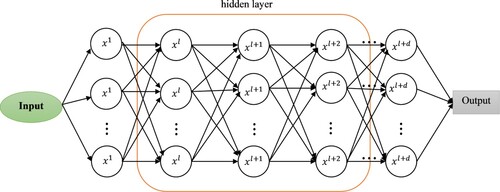
The Universal Approximation Theorem [28] states that an artificial neural network can accurately approximate any closed interval specified in real space. In this work, we applied a multilayer perceptron (MLP) neural network architecture with a layer of input, two layers of hidden n neurons, and an output layer.

Each hidden neuron in Figure 1 is formed as a function that deals with the linear combination of the weight matrix and the neuron's inputs (the learning algorithm optimizes the model parameters $w_i$). The output of each hidden neuron is used as the input of the other neuron, and the output of the neuron of the output layer makes up the output of MLP neural network. The ANN used in this work to solve FDEs (6(6) $\sum _{s=0}^p{P}_s(x,y(x){)}_a{\mathcal{D}}_x^{{\nu }_s}\left[y\right(x\left)\right]=f(x,y\left(x\right)),x\in [a,b]$(6) ) can be mathematically expressed as Equation (11(11) $\sum _{s=0}^p{P}_s{(x,y_0+\sum _{i=0}^m{c}_i{x}^i)}_a{\mathcal{D}}_x^{{\nu }_s}[y_0+\sum _{i=0}^m{c}_i{x}^i]\approx f(x,y_0+\sum _{i=0}^m{c}_i{x}^i),$(11) ).

The interaction between each neuron in the neural architecture can be inferred mathematically as follows: (12) $\begin{array}{rl}{h}_j^{l+k}& =\sigma (\sum _{j=1}^n{w}_j{h}_j^{l-(k-1)}+b_l),k=0,1,\dots ,d\end{array}$(12) (13) $\begin{array}{rl}{c}_i& =\sum _{j=1}^n{v}_j{h}_j^{l+d}+b,\end{array}$(13) where $w^{\prime }s$ and $v^{\prime }s$ denote the weights matrix corresponding to the associated input $x(=h^{l-1})$ and $h^{l+k}$ respectively, $b^{\prime }s$ denotes the bias, σ is the activation functions, and $c_i$ represent the output of the network. Here, we discrete x in the set of points $x_j$ on the interval $[a,b],$ where $j=1,\dots ,n$.

Figure 1. ANN structure for solving FDEs.

The loss function is defined as follows when the neural network is used to compute the numerical solution of problem (6(6) $\sum _{s=0}^p{P}_s(x,y(x){)}_a{\mathcal{D}}_x^{{\nu }_s}\left[y\right(x\left)\right]=f(x,y\left(x\right)),x\in [a,b]$(6) ) (14) $E_j=\frac{1}{2}{(\sum _{s=0}^p{P}_s(x_j,y_0+\sum _{i=0}^m{c}_i{x}^i){\chi }_{s,j}-f(x_j,y_0+\sum _{i=0}^m{c}_i{x}_j^i))}^2+\lambda \Vert w{\Vert }_2^2,$(14) where λ is the known artificial parameter, and $L_2$ is a regularization that helps to push outlier weights nearer 0 but not quite to 0. For ease of expression, the aforementioned mathematical letters ${\chi }_{s,j}$ can be written as below. (15) ${\chi }_{s,j}=\sum _{i=0}^r\frac{\mathrm{\Gamma }(i+1)}{\mathrm{\Gamma }(i+1-{\nu }_s)}{c}_i{x}_j^{i-{\nu }_s},$(15) The parameter $c_i$ is trained through the neural network as shown in Equation (14(14) $E_j=\frac{1}{2}{(\sum _{s=0}^p{P}_s(x_j,y_0+\sum _{i=0}^m{c}_i{x}^i){\chi }_{s,j}-f(x_j,y_0+\sum _{i=0}^m{c}_i{x}_j^i))}^2+\lambda \Vert w{\Vert }_2^2,$(14) ). After that, the value of the right side of (8) can be compared with the value of the left side of (8) and the overall error is obtained by adding the error functions such as (16) $E=\sum _{j=0}^n{E}_j,$(16) then, the following optimization problem is achieved (17) $\begin{array}{r}{\mathrm{a}\mathrm{r}\mathrm{g}\mathrm{m}\mathrm{i}\mathrm{n}}_{a_i}E=\sum _{j=0}^n\frac{1}{2}{(\sum _{s=0}^p{P}_s(x_j,y_0+\sum _{i=0}^m{c}_i{x}^i){\chi }_{s,j}-f(x_j,y_0+\sum _{i=0}^m{c}_i{x}^i))}^2+\lambda \Vert w{\Vert }_2^2.\end{array}$(17) Figure 1 represents the structure of a neural network, and its hidden neurons of the hidden layers are described in Equation (12(12) $\begin{array}{rl}{h}_j^{l+k}& =\sigma (\sum _{j=1}^n{w}_j{h}_j^{l-(k-1)}+b_l),k=0,1,\dots ,d\end{array}$(12) ). Finally, $c_i$ is obtained via the forward propagation of Figure 1. Then substitute $c_i$ and discrete point $x_j$ into both sides of Equation (11(11) $\sum _{s=0}^p{P}_s{(x,y_0+\sum _{i=0}^m{c}_i{x}^i)}_a{\mathcal{D}}_x^{{\nu }_s}[y_0+\sum _{i=0}^m{c}_i{x}^i]\approx f(x,y_0+\sum _{i=0}^m{c}_i{x}^i),$(11) ), and execute Equation (14(14) $E_j=\frac{1}{2}{(\sum _{s=0}^p{P}_s(x_j,y_0+\sum _{i=0}^m{c}_i{x}^i){\chi }_{s,j}-f(x_j,y_0+\sum _{i=0}^m{c}_i{x}_j^i))}^2+\lambda \Vert w{\Vert }_2^2,$(14) ). Equation (11(11) $\sum _{s=0}^p{P}_s{(x,y_0+\sum _{i=0}^m{c}_i{x}^i)}_a{\mathcal{D}}_x^{{\nu }_s}[y_0+\sum _{i=0}^m{c}_i{x}^i]\approx f(x,y_0+\sum _{i=0}^m{c}_i{x}^i),$(11) ) serves as a loss function for adjusting $w^{\prime }s$ and $b^{\prime }s$. We employ the ReLU function as the activation function in this neural network because ReLU provides the following benefits. First, it can speed up network training because its derivative is more straightforward to get than the sigmoid and tanh functions. Second, it makes the network more nonlinear, because it is a nonlinear function by nature, when applied to the neural network, It can be a grid-fitting nonlinear mapping. Third, it can also stop the gradient from fading. The derivatives of the sigmoid and tanh functions are near 0 when the value is too high or too low, but since relu is an uncompressed activation function, this occurrence does not occur. Finally, it can decrease overfitting by making the grid sparse because the part less than zero is zero and the part higher than zero has value.

Consequently, we decide to adopt the adaptive moment estimation (Adam) approach to minimize the loss function because it is successful in real-world applications. Compared to other approaches to adaptive learning rate, it has a higher convergence rate and a more reliable learning impact. Additionally, it can fix problems with other optimization methods, including the disappearance of the learning rate, plodding convergence speed, or significant loss function variation brought on by high variance parameter update.

4. Numerical simulations

In this part, we provide three examples to demonstrate the validity and effectiveness of the proposed ANN algorithm. Python 3.9.1 was used to implement all the numerical results in the following examples. In the examples, the proposed architecture of the MLP neural network sets up three hidden layers, the first two have 30-30 hidden neurons, and the third has 3. These hidden layers are fully connected with one input layer and one output layer. This proposed architecture is known as Net.4 in the rest of the paper. Here, the results of Net.4 are compared to Net.1 [22], Net.2 [25], and Net.3 [25]. More details about these neural networks are given in Table 1. We take m = 3 and compute the following mean square error (MSE) in numerical experiments to make comparisons easier. (18) $MSE=\frac{1}{n}\sum _{j=0}^n\left(f\right(x_j)-y_j{)}^2,$(18) where n represents the number of epochs.

Table 1. Structure of the proposed and comparative networks.

Structure	Net.1 [22]	Net.2 [25]	Net.3 [25]	Net.4
Number of hidden layers	1	1	3	3
Number of hidden neurons	3	30	30,30,30	30,30,3
Activation function	ReLU	ReLU	ReLU	ReLU
Learning rate	0.01	0.001	0.001	0.001
Batch size	64	64	64	64
Optimization algorithm	Adam	Adam	Adam	Adam

With the batch size 64, MSE is optimized using the Adam optimizer. Adam is a first-order gradient-based optimization of stochastic loss functions that has found considerable use in fitting intricate deep neural networks [29]. The approach is reliable, computationally practical, and effective when applied to deep neural networks with many parameters. To obtain the optimal optimization result, tuning the learning rate, learning rate warm-up, learning rate schedules, momentum choices, selection of regularizers and their parameters are required.

Example 4.1

Consider the problem of the Bagley–Torvik equation [30] (19) ${}_a{\mathcal{D}}_x^{2}y\left(x\right){+}_a{\mathcal{D}}_x^{1.5}y\left(x\right)=1+x,0<\nu \le 1\mathrm{a}\mathrm{n}\mathrm{d}0\le x\le 1$(19) with the initial conditions $y\left(0\right)=1$ and $y^{\prime }\left(0\right)=1.$

Figure 2 represents the influences of MSE with an increasing number of epochs. It consists of the performance of four networks for n = 6 and n = 11. We can observe that Net.2 and Net.3 have the value of the loss function has a sharp decrease trend, and when increasing the number of epochs then, the value of the loss function fluctuates. However, Net.1 and Net.4 show stable lines after a certain number of epochs, which means the value of the loss function consistently decreases without deteriorating the accuracy. Table 2 consists of the absolute error of $f\left(x\right)-y$ with the epochs of 5000, where $f\left(x\right)$ represent the exact solutions associated with the sample x and y is the approximate solutions for Net.1, Net.2, Net.3, and Net.4. Net.4 achieved higher accuracy than the other comparative networks. The exact and approximation solutions are represented in Figure 3. It is confirmed that the suggested Net.4 works effectively since the curve of the exact solution almost precisely coincides with the curve of the approximate solutions.

Figure 2. Performances of the networks with the number of epochs (a) n = 6 (b) n = 11.

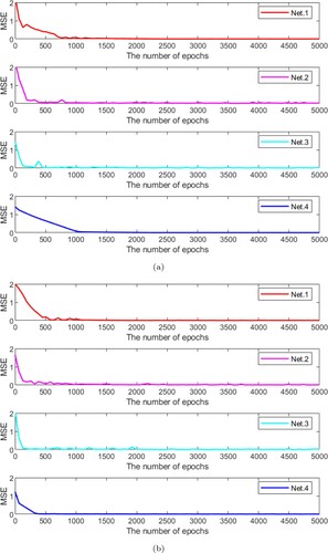
Figure 3. Exact and approximate solutions with the epoch 5000 (a) n = 6 (b) n = 11.

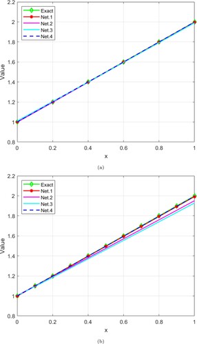
Table 2. Absolute error of $f\left(x\right)-y$ for epoch = 5000.

x	$f\left(x\right)$	Net.1 [22]	Net.2 [25]	Net.3 [25]	Net.4
	n = 6
0	1	4.4100E−04	2.0390E−03	9.5410E−03	2.7000E−05
0.2	1.2	8.1400E−04	3.0510E−03	4.3650E−03	3.3000E−05
0.4	1.4	1.1980E−03	3.9290E−03	2.2460E−03	4.3000E−05
0.6	1.6	1.6040E−03	4.7760E−03	4.1100E−03	5.8000E−05
0.8	1.8	2.0420E−03	5.6950E−03	7.0420E−03	7.9000E−05
1	2	2.5250E−03	6.7890E−03	8.8610E−03	1.0700E−04
	n = 11
0	1	2.1650E−03	4.0900E−03	2.7500E−03	1.6600E−04
0.1	1.1	2.3580E−03	1.6550E−03	5.6680E−03	8.1600E−04
0.2	1.2	2.5710E−03	7.3500E−03	1.3946E−02	1.4740E−03
0.3	1.3	2.7980E−03	1.2971E−02	2.2047E−02	2.1380E−03
0.4	1.4	3.0360E−03	1.8489E−02	2.9934E−02	2.8090E−03
0.5	1.5	3.4890E−03	2.3881E−02	3.7571E−02	3.2810E−03
0.6	1.6	4.1750E−03	2.9120E−02	4.4919E−02	3.5290E−03
0.7	1.7	4.8700E−03	3.4180E−02	5.1944E−02	3.7760E−03
0.8	1.8	5.5730E−03	3.9035E−02	5.8606E−02	4.0180E−03
0.9	1.9	6.2840E−03	4.3660E−02	6.4869E−02	4.2520E−03
1	2	7.0040E−03	4.8027E−02	7.0696E−02	4.4730E−03

Example 4.2

Consider the problem of the fractional order Lane-Emden equation [31] (20) ${}_a{\mathcal{D}}_x^{\nu }y\left(x\right)+{\frac{2}{x^{\nu -\eta }}}_a{\mathcal{D}}_x^{\eta }y\left(x\right)+\frac{1}{x^{\nu -2}}y\left(x\right)=g\left(x\right),0\le x\le 1$(20) with $y\left(0\right)=0$, $y^{\prime }\left(0\right)=0$.

In this example, we consider $\nu =1.5$, $\eta =0.5$, and (21) $g\left(x\right)=x^{2-\nu }(6x(\frac{x^2}{6}+\frac{\mathrm{\Gamma }(4-\eta )+2\mathrm{\Gamma }(4-\nu )}{\mathrm{\Gamma }(4-\eta )\mathrm{\Gamma }(4-\nu )})-2(\frac{x^2}{2}+\frac{\mathrm{\Gamma }(3-\eta )+2\mathrm{\Gamma }(3-\nu )}{\mathrm{\Gamma }(3-\eta )\mathrm{\Gamma }(3-\nu )})).$(21) The test Example 4.2 is a special type of fraction differential equation different from Example 4.1. As in the previous Example 4.1, Figure 4 shows the MSE with increasing the number of epochs for proposed architecture (Net.4) and comparative networks (Net.1, Net.2, and Net.3). The absolute error of $f\left(x\right)-y$ is recorded in Table 3. Additionally, Figure 5 plotted the exact and approximation solutions for various numbers of collocation points.

Figure 4. Performances of the networks with the number of epochs (a) n = 5 (b) n = 10.

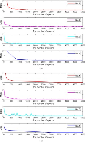
Figure 5. Exact and approximate solutions with the epoch 5000 (a) n = 5 (b) n = 10.

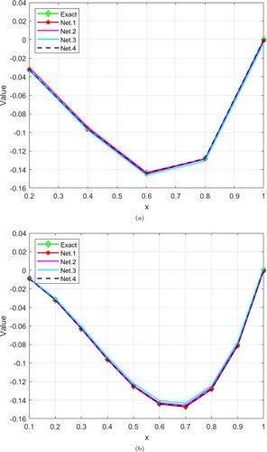
Table 3. Absolute error of $f\left(x\right)-y$ for epoch = 5000.

x	n1.1$f\left(x\right)$	Net.1 [22]	Net.2 [25]	Net.3 [25]	Net.4
	n = 5
0.2	−0.032	5.9700E−04	2.2820E−03	1.2260E−03	3.4000E−05
0.4	−0.096	5.9900E−04	1.7090E−03	1.6500E−03	4.5000E−05
0.6	−0.144	6.4400E−04	8.3100E−04	2.1970E−03	6.1000E−05
0.8	−0.128	7.8100E−04	4.7100E−04	2.9420E−03	8.2000E−05
1	0	1.0660E−03	2.3220E−03	3.9670E−03	1.1200E−04
	n = 10
0.1	−0.009	6.4000E−05	1.1700E−04	7.7700E−04	1.9100E−04
0.2	−0.032	1.8600E−04	7.1900E−04	1.7430E−03	7.9000E−05
0.3	−0.063	2.1200E−04	6.9600E−04	2.2210E−03	9.0000E−05
0.4	−0.096	2.4300E−04	7.4300E−04	2.6980E−03	1.0300E−04
0.5	−0.125	2.8000E−04	8.7000E−04	3.1320E−03	1.1900E−04
0.6	−0.144	3.2500E−04	1.0900E−03	3.4830E−03	1.3800E−04
0.7	−0.147	3.7900E−04	1.4150E−03	3.7090E−03	1.6100E−04
0.8	−0.128	4.4200E−04	1.8560E−03	3.7700E−03	1.8700E−04
0.9	−0.081	5.1500E−04	2.4260E−03	3.6240E−03	2.1800E−04
1	0	5.9900E−04	3.1340E−03	3.2280E−03	2.5300E−04

Example 4.3

Consider the problem of the higher order nonlinear FDE [32] (22) ${}_a{\mathcal{D}}_x^{3}y\left(x\right){+}_a{\mathcal{D}}_x^{2.5}y\left(x\right)+y^2\left(x\right)=x^4,0<\nu \le 1\mathrm{a}\mathrm{n}\mathrm{d}0\le x\le 1$(22) with $y\left(0\right)=0$, $y^{\prime }\left(0\right)=0$, and $y^{″}\left(0\right)=2$.

The test Example 4.3 is a higher order nonlinear fractional differential equation different from the previous test Examples 4.1 & 4.2. As in the previous examples, Figure 6, Table 4, and Figure 7 display the same results.

Figure 6. Performances of the networks with the number of epochs (a) n = 6 (b) n = 11.

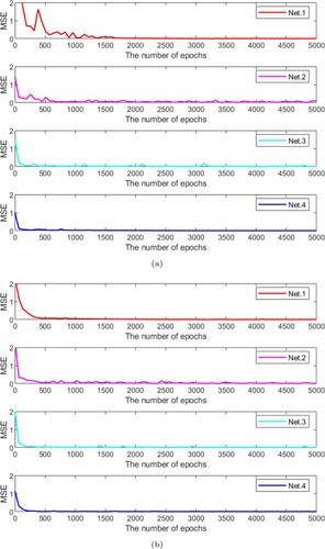
Figure 7. Exact and approximate solutions with the epoch 5000 (a) n = 6 (b) n = 11.

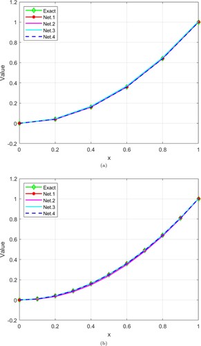
Table 4. Absolute error of $f\left(x\right)-y$ for epoch = 5000.

x	$f\left(x\right)$	Net.1 [22]	Net.2 [25]	Net.3 [25]	Net.4
	n = 6
0	0	6.6000E−05	1.8900E−04	2.2000E−05	2.0000E−05
0.2	0.04	2.4400E−04	3.8700E−04	5.1170E−03	2.5000E−05
0.4	0.16	6.1700E−04	2.2600E−04	8.5000E−03	3.2000E−05
0.6	0.36	1.0150E−03	5.4400E−04	1.0226E−02	4.3000E−05
0.8	0.64	1.4020E−03	2.1800E−03	1.0349E−02	5.9000E−05
1	1	1.7430E−03	4.9350E−03	8.9230E−03	8.1000E−05
	n = 11
0	0	5.6800E−04	2.6450E−03	6.9400E−04	7.2000E−05
0.1	0.01	6.5300E−04	2.1640E−03	1.6720E−03	1.3000E−05
0.2	0.04	7.3600E−04	5.9370E−03	2.5040E−03	1.0600E−04
0.3	0.09	8.2100E−04	8.6800E−03	3.1930E−03	2.0600E−04
0.4	0.16	9.1400E−04	1.0399E−02	3.7420E−03	3.1400E−04
0.5	0.25	1.0170E−03	1.1099E−02	4.1540E−03	4.2700E−04
0.6	0.36	1.1360E−03	1.0786E−02	4.4310E−03	5.4600E−04
0.7	0.49	1.2740E−03	9.4650E−03	4.5780E−03	6.7100E−04
0.8	0.64	1.4350E−03	7.1430E−03	4.5960E−03	8.0100E−04
0.9	0.81	1.6250E−03	3.8250E−03	4.4890E−03	9.3600E−04
1	1	1.8460E−03	4.8300E−04	4.2590E−03	1.0750E−03

5. Conclusion

This paper suggests an ANN architecture to solve fractional differential equations. The advantages of the proposed ANN algorithm are examined using the three different fractional differential equations, including a higher-order nonlinear fractional differential equation. The proposed neural network architecture finds more accuracy than the comparative neural networks (Net.1 [22], Net.2 [25], Net.3 [25]) in the test examples considered and could get a more satisfactory approximate solution with non-mesh discretization. The result obtained here is more accurate compared to existing results obtained in the available literature. We have uploaded the main source code on GitHub: https://github.com/amanojup/FDEsANN.git. The methodology described in this article can be applied to other types of challenging fractional-type problems.

Acknowledgments

The researchers would like to acknowledge Deanship of Scientific Research, Taif University for funding this work. Further authors are grateful to reviewers for their fruitful comments. Manoj Kumar are thankful to UGC for providing SRF.

Disclosure statement

No potential conflict of interest was reported by the author(s).

References

- Baleanu D, Diethelm K, Scalas E, et al. Fractional calculus: models and numerical methods. Vol. 3. New Jersey (NJ): World Scientific; 2012.
- Baleanu D, Güvenç ZB, Machado JT, et al. New trends in nanotechnology and fractional calculus applications. Vol. 10. New York (NY): Springer; 2010.
- Bazhlekova E, Bazhlekov I. Viscoelastic flows with fractional derivative models: computational approach by convolutional calculus of dimovski. Fract Calc Appl Anal. 2014;17(4):954–976.
- Arqub OA, Al-Smadi M. An adaptive numerical approach for the solutions of fractional advection–diffusion and dispersion equations in singular case under riesz's derivative operator. Phys A Stat Mech Appl. 2020;540:Article ID 123257.
- Su X, Xu W, Chen W, et al. Fractional creep and relaxation models of viscoelastic materials via a non-newtonian time-varying viscosity: physical interpretation. Mech Mater. 2020;140:Article ID 103222.
- Stefański TP, Gulgowski J. Signal propagation in electromagnetic media described by fractional-order models. Commun Nonlinear Sci Numer Simul. 2020;82:Article ID 105029.
- Baleanu D, Shekari P, Torkzadeh L, et al. Stability analysis and system properties of nipah virus transmission: A fractional calculus case study. Chaos Solitons Fract. 2023;166:Article ID 112990.
- Baleanu D, Jajarmi A, Mohammadi H, et al. A new study on the mathematical modelling of human liver with caputo–fabrizio fractional derivative. Chaos Solitons Fract. 2020;134:Article ID 109705.
- Jajarmi A, Baleanu D, Sajjadi SS, et al. Analysis and some applications of a regularized ψ–hilfer fractional derivative. J Comput Appl Math. 2022;415.
- Baleanu D, Ghassabzade FA, Nieto JJ, et al. On a new and generalized fractional model for a real cholera outbreak. Alex Eng J. 2022;61(11):9175–9186.
- Defterli O, Baleanu D, Jajarmi A, et al. Fractional treatment: an accelerated mass-spring system. Rom Rep Phys. 2022;74:122.
- Lagaris IE, Likas AC, Papageorgiou DG. Neural-network methods for boundary value problems with irregular boundaries. IEEE Trans Neural Netw. 2000;11(5):1041–1049.
- Sabir Z, Said SB, Al-Mdallal Q, et al. A neuro swarm procedure to solve the novel second order perturbed delay lane-emden model arising in astrophysics. Sci Rep. 2022;12(1):1–15.
- Sabir Z, Said SB. Heuristic computing for the novel singular third order perturbed delay differential model arising in thermal explosion theory. Arab J Chem. 2023;16(3):Article ID 104509.
- Sabir Z, Botmart T, Raja MAZ, et al. A stochastic numerical approach for a class of singular singularly perturbed system. PLoS One. 2022;17(11):e0277291.
- Sabir Z, Said SB, Baleanu D. Swarming optimization to analyze the fractional derivatives and perturbation factors for the novel singular model. Chaos Solitons Fract. 2022;164:Article ID 112660.
- Sabir Z, Raja MAZ, Ali MR, et al. An advance computational intelligent approach to solve the third kind of nonlinear pantograph lane–emden differential system. Evol Syst. 2022;12:1–20.
- Sabir Z, Wahab HA, Nguyen TG, et al. Intelligent computing technique for solving singular multi-pantograph delay differential equation. Soft Comput. 2022;16:1–13.
- Chen F, Sondak D, Protopapas P, et al. Neurodiffeq: A python package for solving differential equations with neural networks. J Open Source Softw. 2020;5(46):1931.
- Wu M, Zhang J, Huang Z, et al. Numerical solutions of wavelet neural networks for fractional differential equations. Math Methods Appl Sci. 2021;46:3031–3044.
- Gao F, Dong Y, Chi C. Solving fractional differential equations by using triangle neural network. J Funct Spaces. 2021;2021:1–7.
- Rostami F, Jafarian A. A new artificial neural network structure for solving high-order linear fractional differential equations. Int J Comput Math. 2018;95:528–539.
- Pakdaman M, Ahmadian A, Effati S, et al. Solving differential equations of fractional order using an optimization technique based on training artificial neural network. Appl Math Comput. 2017;293:81–95.
- Hadian-Rasanan AH, Rahmati D, Gorgin S, et al. A single layer fractional orthogonal neural network for solving various types of lane–emden equation. New Astron. 2020;75:Article ID 101307.
- Dai P, Yu X. An artificial neural network approach for solving space fractional differential equations. Symmetry. 2022;14(3):535.
- Singh R. Optimal homotopy analysis method for the non-isothermal reaction–diffusion model equations in a spherical catalyst. J Math Chem. 2018;56(9):2579–2590.
- Singh R. Analytical approach for computation of exact and analytic approximate solutions to the system of lane-emden-fowler type equations arising in astrophysics. Eur Phys J Plus. 2018;133(8):1–12.
- Hornik K. Approximation capabilities of multilayer feedforward networks. Neural Netw. 1991;4(2):251–257.
- Kingma D, Ba J. Adam: A Method for Stochastic Optimization. San Diego 3rd International Conference for Learning Representations. 2015.
- Momani S, Odibat Z. Numerical comparison of methods for solving linear differential equations of fractional order. Chaos Solitons Fract. 2007;31(5):1248–1255.
- Akgül A, Inc M, Karatas E, et al. Numerical solutions of fractional differential equations of lane-emden type by an accurate technique. Adv Differ Equ. 2015;2015(1):1–12.
- Deshi A, Gudodagi G. Numerical solution of Bagley–Torvik, nonlinear and higher order fractional differential equations using haar wavelet. SeMA J. 2022;79(4):663–675.