Landweber iterative regularization method for an inverse initial value problem of diffusion equation with local and nonlocal operators

ABSTRACT

This paper considers an inverse initial value problem of diffusion equation with local and nonlocal operators. For this ill-posed problem, we give and prove a result of conditional stability. Meanwhile, Landweber iterative regularization method is used to overcome the ill-posedness, and based on the result of conditional stability, the convergence estimates of Hölder type for regularization method are derived under the a-priori and a-posteriori choice rules for the regularized parameter. Finally, some numerical results are provided to show that Landweber iterative method works well in solving this inverse problem.

KEYWORDS:

• Inverse initial value problem
• diffusion equation with local and nonlocal operators
• Landweber regularization
• convergence estimate
• numerical implementation

MATHEMATICS SUBJECT CLASSIFICATIONS:

• 35R25
• 35R30
• 26A33
• 65N20
• 47J06

1. Introduction

In this paper, we consider the inverse initial value problem of diffusion equation with local and nonlocal operators (1) $\begin{array}{r}\{\begin{array}{ll}{u}_t(x,t)-\alpha \mathrm{\Delta }u(x,t)+\beta (-\mathrm{\Delta }{)}^{\gamma }u(x,t)=\ell (x,t),& x\in \mathbb{R},t\in (0,T),\\ u(x,T)=\vartheta (x),& x\in \mathbb{R},\end{array}\end{array}$(1) where, $\alpha ,\beta >0$ are the diffusion coefficients, $\gamma \in (0,1)$ is the fractional order of nonlocal Laplacian, and the nonlocal Laplacian of one-dimension is defined pointwise by the principal value integral [1] (2) $\begin{array}{r}(-△{)}^{\gamma }f(x)=c_{\gamma }P.V.{\int }_{\mathbb{R}}\frac{f(x)-f(y)}{|x-y{|}^{1+2\gamma }}\mathrm{d}y,\end{array}$(2) $c_{\gamma }$ is a constant, $P.V.{\int }_{\mathbb{R}}\frac{f(x)-f(y)}{|x-y{|}^{1+2\gamma }}\mathrm{d}y=\underset{\xi \to 0}{lim}{\int }_{\mathbb{R}\mathrm{\setminus }(|x-y|\le \xi )}\frac{f(x)-f(y)}{|x-y{|}^{1+2\gamma }}\mathrm{d}y$. The nonlocal Laplacian $(-△{)}^{\gamma }$ also can be defined equivalently through the inverse Fourier transform (3) $\begin{array}{r}(-△{)}^{\gamma }f(x):={\mathcal{F}}^{-1}(|\xi {|}^{2\gamma }(\mathcal{F}f)(\xi ))(x),\end{array}$(3) where $\mathcal{F}$ dontes the Fourier transform operator which is defined by (4) $\begin{array}{r}(\mathcal{F}f)(\xi ):=\hat{f}(\xi )=\frac{1}{\sqrt{2\pi }}{\int }_{\mathbb{R}}f(x){\mathrm{e}}^{-i\xi x}\mathrm{d}x.\end{array}$(4) $\vartheta (x)$, $\ell (x,t)$ denotes the exact final data and source function, let $\delta >0$ be the bound of measured error, ${\vartheta }^{\delta }(x)$, ${\ell }^{\delta }(x,t)$ be the measured final data and source function, which satisfy (5) $\begin{array}{rl}& {\Vert {\vartheta }^{\delta }(x)-\vartheta (x)\Vert }_{L^2(\mathbb{R})}\le \delta ,\end{array}$(5) (6) $\begin{array}{rl}& {\Vert {\ell }^{\delta }(x,t)-\ell (x,t)\Vert }_{L^2(0,T;L^2(\mathbb{R}))}\le \delta .\end{array}$(6) Our task is to realize the inversion of initial value $u(x,0)$ from the measured datum ${\vartheta }^{\delta }(x)$ and ${\ell }^{\delta }(x,t)$.

We know that, as $\alpha >0$, $\beta =0$, the main equation in (1(1) $\begin{array}{r}\{\begin{array}{ll}{u}_t(x,t)-\alpha \mathrm{\Delta }u(x,t)+\beta (-\mathrm{\Delta }{)}^{\gamma }u(x,t)=\ell (x,t),& x\in \mathbb{R},t\in (0,T),\\ u(x,T)=\vartheta (x),& x\in \mathbb{R},\end{array}\end{array}$(1) ) is just the classical diffusion equation $u_t(x,t)-\alpha \mathrm{\Delta }u(x,t)=\ell (x,t)$, this equation is usually used to describe the density distribution of particles in Brownian motion. For the inverse initial value problem of classical diffusion equation, it had been extensively researched in the past decades, and many regularization methods had been proposed to deal with this ill-posed problem, please see [2–9], etc. On the other hand, as $\alpha =0,\beta >0$, the main equation in (1(1) $\begin{array}{r}\{\begin{array}{ll}{u}_t(x,t)-\alpha \mathrm{\Delta }u(x,t)+\beta (-\mathrm{\Delta }{)}^{\gamma }u(x,t)=\ell (x,t),& x\in \mathbb{R},t\in (0,T),\\ u(x,T)=\vartheta (x),& x\in \mathbb{R},\end{array}\end{array}$(1) ) can be written as the nonlocal (space-fractional) diffusion equation $u_t(x,t)+\beta (-\mathrm{\Delta }{)}^{\gamma }u(x,t)=\ell (x,t)$, which often describes the diffusion law of particles driven by a Lévy flights. On the inverse initial value problem of nonlocal (space-fractional) diffusion equation, there also have some meaningful research works in which some regularization methods have been developed, such as the convolution and spectral methods [10], iteration method [11], simplified Tikhonov method [12,13], logarithmic, negative exponential and fractional Tikhonov methods [14–16], optimal method [17], modified kernel method [18,19], generalized Tikhonov method [20], truncated regularization method [21], and so on.

Recent years, mathematical models that contain the local and nonlocal diffusion operators have attracted the extensive attention of scientists. In this situation, the main equation in (1(1) $\begin{array}{r}\{\begin{array}{ll}{u}_t(x,t)-\alpha \mathrm{\Delta }u(x,t)+\beta (-\mathrm{\Delta }{)}^{\gamma }u(x,t)=\ell (x,t),& x\in \mathbb{R},t\in (0,T),\\ u(x,T)=\vartheta (x),& x\in \mathbb{R},\end{array}\end{array}$(1) ) can be expressed as $u_t(x,t)+\alpha (-\mathrm{\Delta })u(x,t)+\beta (-\mathrm{\Delta }{)}^{\gamma }u(x,t)=\ell (x,t)$, and it describes the diffusion law of particles that follow the Lévy and Brownian processes simultaneously, please see [22]. At present, the model above has been used in many practical application fields, such as the modelling of biological population dynamic [23,24], plasma physics [25–27], the model of light-sensitive Belousov-Zhabotinsky reaction in chemistry [2,14], and so on. For the research works in theoretical aspects on the mathematical models that contain the local and nonlocal diffusion operators, we can see [26–29], etc.

On the inverse initial value problem of diffusion equation with local and nonlocal operators (i.e. problem (1(1) $\begin{array}{r}\{\begin{array}{ll}{u}_t(x,t)-\alpha \mathrm{\Delta }u(x,t)+\beta (-\mathrm{\Delta }{)}^{\gamma }u(x,t)=\ell (x,t),& x\in \mathbb{R},t\in (0,T),\\ u(x,T)=\vartheta (x),& x\in \mathbb{R},\end{array}\end{array}$(1) )), in 2022, the literature [30] developed and used a fractional filter regularization method to overcome its ill-posedness, and derives the a-priori convergence result of logarithmic type. To the authors' best knowledge, except for [30], there are no works published concerning the regularization theory and algorithm of problem (1(1) $\begin{array}{r}\{\begin{array}{ll}{u}_t(x,t)-\alpha \mathrm{\Delta }u(x,t)+\beta (-\mathrm{\Delta }{)}^{\gamma }u(x,t)=\ell (x,t),& x\in \mathbb{R},t\in (0,T),\\ u(x,T)=\vartheta (x),& x\in \mathbb{R},\end{array}\end{array}$(1) ). Based on this research status, this paper continues to consider the inverse initial value problem (1(1) $\begin{array}{r}\{\begin{array}{ll}{u}_t(x,t)-\alpha \mathrm{\Delta }u(x,t)+\beta (-\mathrm{\Delta }{)}^{\gamma }u(x,t)=\ell (x,t),& x\in \mathbb{R},t\in (0,T),\\ u(x,T)=\vartheta (x),& x\in \mathbb{R},\end{array}\end{array}$(1) ). First, based on the ill-posedness analysis, the result of conditional stability of inverse problem will be given and proven. And then, we construct the Landweber iterative method to recover the stability of solution on measured datum. Meanwhile, with the help of conditional stability results, the a-prior and a-posterior convergence results for regularized method are derived, respectively. Finally, by using the discrete Fourier transform and discrete inverse Fourier transform technique, we solve a direct problem to construct the exact datum, and compute the exact and regularized solutions through respective analytic expression, and under the a-priori and a-posteriori cases we respectively verify the simulation effect of Landweber iterative method in solving the considered problem.

The rest of this article is arranged as below. In Section 2, we give the ill-posedness analysis and conditional stability estimate for problem (1(1) $\begin{array}{r}\{\begin{array}{ll}{u}_t(x,t)-\alpha \mathrm{\Delta }u(x,t)+\beta (-\mathrm{\Delta }{)}^{\gamma }u(x,t)=\ell (x,t),& x\in \mathbb{R},t\in (0,T),\\ u(x,T)=\vartheta (x),& x\in \mathbb{R},\end{array}\end{array}$(1) ). Section 3 describes the construction of Landweber iterative regularization method, and derives the a-priori and a-posteriori convergence estimates of regularization method. Section 4 makes some numerical experiments to verify the simulation effect of regularized method. Some conclusions are drawn in Section 5.

2. Ill-posedness of inverse problem and conditional stability

2.1. Ill-posedness of inverse problem

In this subsection, we briefly analyse the ill-posedness of problem (1(1) $\begin{array}{r}\{\begin{array}{ll}{u}_t(x,t)-\alpha \mathrm{\Delta }u(x,t)+\beta (-\mathrm{\Delta }{)}^{\gamma }u(x,t)=\ell (x,t),& x\in \mathbb{R},t\in (0,T),\\ u(x,T)=\vartheta (x),& x\in \mathbb{R},\end{array}\end{array}$(1) ). By taking the Fourier transform with respect to x, and combining with the formula (7) $\begin{array}{r}\widehat{(-△{)}^{\gamma }}u(\xi ,t)=|\xi {|}^{2\gamma }\hat{u}(\xi ,t),\end{array}$(7) we can obtain the following representation in the frequency domain (8) $\begin{array}{r}\hat{u}(\xi ,t)={\mathrm{e}}^{(\alpha |\xi {|}^2+\beta |\xi {|}^{2\gamma })(T-t)}\hat{\vartheta }(\xi )-{\int }_t^T{\mathrm{e}}^{(\alpha |\xi {|}^2+\beta |\xi {|}^{2\gamma })(\sigma -t)}\hat{\ell }(\xi ,\sigma )\mathrm{d}\sigma .\end{array}$(8) Using the inverse Fourier transform, the solution of problem (1(1) $\begin{array}{r}\{\begin{array}{ll}{u}_t(x,t)-\alpha \mathrm{\Delta }u(x,t)+\beta (-\mathrm{\Delta }{)}^{\gamma }u(x,t)=\ell (x,t),& x\in \mathbb{R},t\in (0,T),\\ u(x,T)=\vartheta (x),& x\in \mathbb{R},\end{array}\end{array}$(1) ) can be written as (9) $\begin{array}{r}u(x,t)=\frac{1}{\sqrt{2\pi }}{\int }_{-\mathrm{\infty }}^{\mathrm{\infty }}({\mathrm{e}}^{(\alpha |\xi {|}^2+\beta |\xi {|}^{2\gamma })(T-t)}\hat{\vartheta }(\xi )-{\int }_t^T{\mathrm{e}}^{(\alpha |\xi {|}^2+\beta |\xi {|}^{2\gamma })(\sigma -t)}\hat{\ell }(\xi ,\sigma )\mathrm{d}\sigma ){\mathrm{e}}^{i\xi x}\mathrm{d}\xi .\end{array}$(9) From (8(8) $\begin{array}{r}\hat{u}(\xi ,t)={\mathrm{e}}^{(\alpha |\xi {|}^2+\beta |\xi {|}^{2\gamma })(T-t)}\hat{\vartheta }(\xi )-{\int }_t^T{\mathrm{e}}^{(\alpha |\xi {|}^2+\beta |\xi {|}^{2\gamma })(\sigma -t)}\hat{\ell }(\xi ,\sigma )\mathrm{d}\sigma .\end{array}$(8) ), when t = 0, the solution of problem (1(1) $\begin{array}{r}\{\begin{array}{ll}{u}_t(x,t)-\alpha \mathrm{\Delta }u(x,t)+\beta (-\mathrm{\Delta }{)}^{\gamma }u(x,t)=\ell (x,t),& x\in \mathbb{R},t\in (0,T),\\ u(x,T)=\vartheta (x),& x\in \mathbb{R},\end{array}\end{array}$(1) ) in the frequency domain can be expressed as (10) $\begin{array}{r}\hat{u}(\xi ,0)={\mathrm{e}}^{(\alpha |\xi {|}^2+\beta |\xi {|}^{2\gamma })T}[\hat{\vartheta }(\xi )-{\int }_0^T{\mathrm{e}}^{(\alpha |\xi {|}^2+\beta |\xi {|}^{2\gamma })(\sigma -T)}\hat{\ell }(\xi ,\sigma )\mathrm{d}\sigma ],\end{array}$(10) therefore, by the inverse Fourier transform, as t = 0, the solution of inverse problem can be written as (11) $\begin{array}{r}u(x,0)=\frac{1}{\sqrt{2\pi }}{\int }_{-\mathrm{\infty }}^{\mathrm{\infty }}({\mathrm{e}}^{(\alpha |\xi {|}^2+\beta |\xi {|}^{2\gamma })T}[\hat{\vartheta }(\xi )-{\int }_0^T{\mathrm{e}}^{(\alpha |\xi {|}^2+\beta |\xi {|}^{2\gamma })(\sigma -T)}\hat{\ell }(\xi ,\sigma )\mathrm{d}\sigma ]){\mathrm{e}}^{i\xi x}\mathrm{d}\xi .\end{array}$(11) In the current paper, our task is to realize the inversion of initial value $u(x,0)$ from the measured datum ${\vartheta }^{\delta }(x)$ and ${\ell }^{\delta }(x,t)$ that satisfy (5(5) $\begin{array}{rl}& {\Vert {\vartheta }^{\delta }(x)-\vartheta (x)\Vert }_{L^2(\mathbb{R})}\le \delta ,\end{array}$(5) ) and (6(6) $\begin{array}{rl}& {\Vert {\ell }^{\delta }(x,t)-\ell (x,t)\Vert }_{L^2(0,T;L^2(\mathbb{R}))}\le \delta .\end{array}$(6) ). From (10(10) $\begin{array}{r}\hat{u}(\xi ,0)={\mathrm{e}}^{(\alpha |\xi {|}^2+\beta |\xi {|}^{2\gamma })T}[\hat{\vartheta }(\xi )-{\int }_0^T{\mathrm{e}}^{(\alpha |\xi {|}^2+\beta |\xi {|}^{2\gamma })(\sigma -T)}\hat{\ell }(\xi ,\sigma )\mathrm{d}\sigma ],\end{array}$(10) ) and (11(11) $\begin{array}{r}u(x,0)=\frac{1}{\sqrt{2\pi }}{\int }_{-\mathrm{\infty }}^{\mathrm{\infty }}({\mathrm{e}}^{(\alpha |\xi {|}^2+\beta |\xi {|}^{2\gamma })T}[\hat{\vartheta }(\xi )-{\int }_0^T{\mathrm{e}}^{(\alpha |\xi {|}^2+\beta |\xi {|}^{2\gamma })(\sigma -T)}\hat{\ell }(\xi ,\sigma )\mathrm{d}\sigma ]){\mathrm{e}}^{i\xi x}\mathrm{d}\xi .\end{array}$(11) ), we note that, (12) $\begin{array}{r}\underset{|\xi |\to \mathrm{\infty }}{lim}{\mathrm{e}}^{(\alpha |\xi {|}^2+\beta |\xi {|}^{2\gamma })T}=+\mathrm{\infty },\end{array}$(12) then, the inversion problem of initial value $u(x,0)$ is highly ill-posed, that is, a small perturbation in the measured datum ${\vartheta }^{\delta }(x)$ and ${\ell }^{\delta }(x,t)$ may result in a dramatic error on the solution (or the solution at t = 0 does not continuously depend on the given data). But if it satisfies certain a-priori condition, one can establish the conditional stability of solution at t = 0.

2.2. Conditional stability

In this subsection, under an a-priori assumption of exact solution we are devoted to establish a result of conditional stability for inverse initial value problem. Due to (10(10) $\begin{array}{r}\hat{u}(\xi ,0)={\mathrm{e}}^{(\alpha |\xi {|}^2+\beta |\xi {|}^{2\gamma })T}[\hat{\vartheta }(\xi )-{\int }_0^T{\mathrm{e}}^{(\alpha |\xi {|}^2+\beta |\xi {|}^{2\gamma })(\sigma -T)}\hat{\ell }(\xi ,\sigma )\mathrm{d}\sigma ],\end{array}$(10) ), we define a linear bounded multiplication operator $\hat{K}:L^2(\mathbb{R})\to L^2(\mathbb{R})$ as below (13) $\begin{array}{r}\hat{K}(\xi )\hat{u}(\xi ,0)={\mathrm{e}}^{-(\alpha |\xi {|}^2+\beta |\xi {|}^{2\gamma })T}\hat{u}(\xi ,0)=\hat{g}(\xi ),\end{array}$(13) here (14) $\begin{array}{r}\hat{g}(\xi )=\hat{\vartheta }(\xi )-{\int }_0^T{\mathrm{e}}^{(\alpha |\xi {|}^2+\beta |\xi {|}^{2\gamma })(\sigma -T)}\hat{\ell }(\xi ,\sigma )\mathrm{d}\sigma ,\end{array}$(14) and (15) $\begin{array}{r}\hat{K}(\xi )={\mathrm{e}}^{-(\alpha |\xi {|}^2+\beta |\xi {|}^{2\gamma })T}.\end{array}$(15) We know that $\hat{K}$ is a self-adjoint operator, thus, $\hat{K}{\hat{K}}^{\ast }={\hat{K}}^{\ast }\hat{K}={\mathrm{e}}^{-2(\alpha |\xi {|}^2+\beta |\xi {|}^{2\gamma })T}$. In order to obtain the conditional stability and a-priori and a-posteriori convergence results of Hölder type, this paper assumes that there exists a constant E>0 such that the solution of inverse problem satisfy the a-priori condition (16) $\begin{array}{r}\Vert u(\cdot ,0){\Vert }_p\le E,\end{array}$(16) where the norm of $\Vert u(\cdot ,0){\Vert }_p$ is defined as (17) $\begin{array}{r}\Vert u(\cdot ,0){\Vert }_p={\left({\int }_{-\mathrm{\infty }}^{\mathrm{\infty }}{\mathrm{e}}^{p(\alpha |\xi {|}^2+\beta |\xi {|}^{2\gamma })T}|\hat{u}(\xi ,0){|}^2\mathrm{d}\xi \right)}^{\frac{1}{2}},2<p<4.\end{array}$(17) Notice that, as p = 0, the norm above is just the-norm in square integrable function space $L^2(\mathbb{R})$. Throughout the article, we denote $\Vert \cdot \Vert$ be $L^2$-norm.

Theorem 2.1

Assume that the solution $u(x,0)$ given by (11(11) $\begin{array}{r}u(x,0)=\frac{1}{\sqrt{2\pi }}{\int }_{-\mathrm{\infty }}^{\mathrm{\infty }}({\mathrm{e}}^{(\alpha |\xi {|}^2+\beta |\xi {|}^{2\gamma })T}[\hat{\vartheta }(\xi )-{\int }_0^T{\mathrm{e}}^{(\alpha |\xi {|}^2+\beta |\xi {|}^{2\gamma })(\sigma -T)}\hat{\ell }(\xi ,\sigma )\mathrm{d}\sigma ]){\mathrm{e}}^{i\xi x}\mathrm{d}\xi .\end{array}$(11) ) satisfies the a-prior condition (16(16) $\begin{array}{r}\Vert u(\cdot ,0){\Vert }_p\le E,\end{array}$(16) ), the exact final data $\vartheta (x)\in L^2(\mathbb{R})$, and source function $\ell (x,t)\in L^2(0,T;L^2(\mathbb{R}))$, then we have the following stability result (18) $\begin{array}{r}\Vert u(x,0){\Vert }_{L^2(\mathbb{R})}\le C_1{E}^{\frac{\gamma +2}{p+\gamma +2}}(\Vert \vartheta {\Vert }_{L^2(\mathbb{R})}^2+T\Vert \ell {\Vert }_{L^2(0,T;L^2(\mathbb{R}))}^2{)}^{\frac{p}{2(p+\gamma +2)}},\end{array}$(18) where $C_1:=2^{\frac{p}{2(p+\gamma +2)}}$.

Proof.

Using the Hölder inequality, we can obtain that $\begin{array}{rl}& \Vert u(x,0){\Vert }^2=\Vert \hat{u}(\xi ,0){\Vert }^2={\int }_{-\mathrm{\infty }}^{\mathrm{\infty }}({\mathrm{e}}^{(\alpha |\xi {|}^2+\beta |\xi {|}^{2\gamma })T}\hat{g}(\xi ){)}^2\mathrm{d}\xi \\ & ={\int }_{-\mathrm{\infty }}^{\mathrm{\infty }}(\hat{g}(\xi ){)}^{\frac{2(\gamma +2)}{p+\gamma +2}}{\mathrm{e}}^{2(\alpha |\xi {|}^2+\beta |\xi {|}^{2\gamma })T}(\hat{g}(\xi ){)}^{\frac{2p}{p+\gamma +2}}\mathrm{d}\xi \\ & \le {({\int }_{-\mathrm{\infty }}^{\mathrm{\infty }}((\hat{g}(\xi ){)}^{\frac{2(\gamma +2)}{p+\gamma +2}}{\mathrm{e}}^{2(\alpha |\xi {|}^2+\beta |\xi {|}^{2\gamma })T}{)}^{\frac{p+\gamma +2}{\gamma +2}}\mathrm{d}\xi )}^{\frac{\gamma +2}{p+\gamma +2}}\\ & {({\int }_{-\mathrm{\infty }}^{\mathrm{\infty }}((\hat{g}(\xi ){)}^{\frac{2p}{p+\gamma +2}}{)}^{\frac{p+\gamma +2}{p}}\mathrm{d}\xi )}^{\frac{p}{p+\gamma +2}}\\ & \le {({\int }_{-\mathrm{\infty }}^{\mathrm{\infty }}(\hat{g}(\xi ){)}^2{\mathrm{e}}^{2\frac{(\alpha |\xi {|}^2+\beta |\xi {|}^{2\gamma })(p+\gamma +2)T}{\gamma +2}}\mathrm{d}\xi )}^{\frac{\gamma +2}{p+\gamma +2}}{({\int }_{-\mathrm{\infty }}^{\mathrm{\infty }}(\hat{g}(\xi ){)}^2\mathrm{d}\xi )}^{\frac{p}{p+\gamma +2}}\\ & =I_1^{\frac{\gamma +2}{p+\gamma +2}}{I}_2^{\frac{p}{p+\gamma +2}}.\end{array}$By the a-pririor condition (16(16) $\begin{array}{r}\Vert u(\cdot ,0){\Vert }_p\le E,\end{array}$(16) ), it can be gotten that $\begin{array}{rl}& I_1={\int }_{-\mathrm{\infty }}^{\mathrm{\infty }}(\hat{g}(\xi ){)}^2{\mathrm{e}}^{2\frac{(\alpha |\xi {|}^2+\beta |\xi {|}^{2\gamma })(p+\gamma +2)T}{\gamma +2}}\mathrm{d}\xi \\ & ={\int }_{-\mathrm{\infty }}^{\mathrm{\infty }}{\mathrm{e}}^{-2(\alpha |\xi {|}^2+\beta |\xi {|}^{2\gamma })T}|\hat{u}(\xi ,0){|}^2{\mathrm{e}}^{(\alpha |\xi {|}^2+\beta |\xi {|}^{2\gamma })pT}{\mathrm{e}}^{-(\alpha |\xi {|}^2+\beta |\xi {|}^{2\gamma })pT}\\ & \times {\mathrm{e}}^{2\frac{(\alpha |\xi {|}^2+\beta |\xi {|}^{2\gamma })(p+\gamma +2)T}{\gamma +2}}\mathrm{d}\xi \\ & ={\int }_{-\mathrm{\infty }}^{\mathrm{\infty }}|\hat{u}(\xi ,0){|}^2{\mathrm{e}}^{(\alpha |\xi {|}^2+\beta |\xi {|}^{2\gamma })pT}{\mathrm{e}}^{(\alpha |\xi {|}^2+\beta |\xi {|}^{2\gamma })Tp(\frac{2}{\gamma +2}-1)}\mathrm{d}\xi \\ & \le E^2,\end{array}$On the other hand, by using the Cauchy Schwartz inequality and basic calculation, we have $\begin{array}{rl}& I_2=\Vert g{\Vert }_{L^2(\mathbb{R})}^2={\int }_{-\mathrm{\infty }}^{\mathrm{\infty }}|\hat{g}(\xi ){|}^2\mathrm{d}\xi \\ & ={\int }_{-\mathrm{\infty }}^{\mathrm{\infty }}{|\hat{\vartheta }(\xi )-{\int }_0^T{\mathrm{e}}^{(\alpha |\xi {|}^2+\beta |\xi {|}^{2\gamma })(\sigma -T)}\hat{\ell }(\xi ,\sigma )\mathrm{d}\sigma |}^2\mathrm{d}\xi \\ & \le {\int }_{-\mathrm{\infty }}^{\mathrm{\infty }}(2|\hat{\vartheta }(\xi ){|}^2+2{|{\int }_0^T{\mathrm{e}}^{(\alpha |\xi {|}^2+\beta |\xi {|}^{2\gamma })(\sigma -T)}\hat{\ell }(\xi ,\sigma )\mathrm{d}\sigma |}^2)\mathrm{d}\xi \\ & =2{\int }_{-\mathrm{\infty }}^{\mathrm{\infty }}|\hat{\vartheta }(\xi ){|}^2\mathrm{d}\xi +2{\int }_{-\mathrm{\infty }}^{\mathrm{\infty }}{|{\int }_0^T{\mathrm{e}}^{(\alpha |\xi {|}^2+\beta |\xi {|}^{2\gamma })(\sigma -T)}\hat{\ell }(\xi ,\sigma )\mathrm{d}\sigma |}^2\mathrm{d}\xi \\ & \le 2\Vert \vartheta {\Vert }_{L^2(\mathbb{R})}^2+2{\int }_{-\mathrm{\infty }}^{\mathrm{\infty }}{\left({\int }_0^T|{\mathrm{e}}^{(\alpha |\xi {|}^2+\beta |\xi {|}^{2\gamma })(\sigma -T)}\hat{\ell }(\xi ,\sigma )|\mathrm{d}\sigma \right)}^2\mathrm{d}\xi \\ & \le 2\Vert \vartheta {\Vert }_{L^2(\mathbb{R})}^2+2{\int }_{-\mathrm{\infty }}^{\mathrm{\infty }}{\left({\int }_0^T|\hat{\ell }(\xi ,\sigma )|\mathrm{d}\sigma \right)}^2\mathrm{d}\xi \\ & \le 2\Vert \vartheta {\Vert }_{L^2(\mathbb{R})}^2+2{\int }_{-\mathrm{\infty }}^{\mathrm{\infty }}\left(T{\int }_0^T{|\hat{\ell }(\xi ,\sigma )|}^2\mathrm{d}\sigma \right)\mathrm{d}\xi \\ & \le 2\Vert \vartheta {\Vert }_{L^2(\mathbb{R})}^2+2T{\int }_0^T{\int }_{-\mathrm{\infty }}^{\mathrm{\infty }}{|\hat{\ell }(\xi ,\sigma )|}^2\mathrm{d}\xi \mathrm{d}\sigma \\ & \le 2(\Vert \hat{\vartheta }{\Vert }_{L^2(\mathbb{R})}^2+T\Vert \ell {\Vert }_{L^{2(0,T;L^2(\mathbb{R}))}}^2).\end{array}$Finally, according the estimates of $I_1$ and $I_2$, we obtain that $\Vert u(x,0){\Vert }_{L^2(\mathbb{R})}\le C_1{E}^{\frac{\gamma +2}{p+\gamma +2}}{(\Vert \vartheta {\Vert }_{L^2(\mathbb{R})}^2+T\Vert \ell {\Vert }_{L^2(0,T;L^2(\mathbb{R}))}^2)}^{\frac{p}{2(p+\gamma +2)}}.$

3. Landweber iterative method and convergence estimates

This section firstly describes the construction of Landweber iterative regularization method in dealing with the inverse initial value problem (1(1) $\begin{array}{r}\{\begin{array}{ll}{u}_t(x,t)-\alpha \mathrm{\Delta }u(x,t)+\beta (-\mathrm{\Delta }{)}^{\gamma }u(x,t)=\ell (x,t),& x\in \mathbb{R},t\in (0,T),\\ u(x,T)=\vartheta (x),& x\in \mathbb{R},\end{array}\end{array}$(1) ), and the convergence estimates of Hölder type under the a-priori and a-posteriori choice rules for regularized parameter are obtained.

3.1. Landweber iterative regularization method

According to the idea of general regularization theory in [31,32], we use the equation $\hat{u}(\xi ,0)=(I-a{\hat{K}}^{\ast }\hat{K})\hat{u}(\xi ,0)+a{\hat{K}}^{\ast }\hat{g}(\xi )$ to replace the operator equation in (13(13) $\begin{array}{r}\hat{K}(\xi )\hat{u}(\xi ,0)={\mathrm{e}}^{-(\alpha |\xi {|}^2+\beta |\xi {|}^{2\gamma })T}\hat{u}(\xi ,0)=\hat{g}(\xi ),\end{array}$(13) ) $\hat{K}(\xi )\hat{u}(\xi ,0)=\hat{g}(\xi )$, and let ${\hat{g}}^{\delta }(\xi )={\hat{\vartheta }}^{\delta }(\xi )-{\int }_0^T{\mathrm{e}}^{(\alpha |\xi {|}^2+\beta |\xi {|}^{2\gamma })(\sigma -T)}{\hat{\ell }}^{\delta }(\xi ,\sigma )\mathrm{d}\sigma$ be the noisy data, then one can get the following iterative format (19) $\begin{array}{rl}& {\hat{u}}^{0,\delta }(\xi ,0)=0,\\ & {\hat{u}}^{m,\delta }(\xi ,0)=(I-a{\hat{K}}^{\ast }\hat{K}){\hat{u}}^{m-1,\delta }(\xi ,0)+a{\hat{K}}^{\ast }{\hat{g}}^{\delta }(\xi ),m=1,2,3,\dots ,\end{array}$(19) where, ${\hat{u}}^{m,\delta }(\xi ,0)$ is called the Landweber iterative regularization solution with error data in the frequency domain, I is a unit operator, m is the iterative step number, a denotes the relaxation factor that satisfies $0<a<\frac{1}{\Vert \hat{K}{\Vert }^2}$. Since $\hat{K}$ is a self-adjoint operator, we denote operator $R_m$: $L^2(\mathbb{R})\to L^2(\mathbb{R})$ as follows $R_m=a\sum _{k=0}^{m-1}(I-a{\hat{K}}^{\ast }\hat{K}{)}^k{\hat{K}}^{\ast },m=1,2,3,\dots .$By the basic calculation, we obtain (20) $\begin{array}{r}{\hat{u}}^{m,\delta }(\xi ,0)=R_m{\hat{g}}^{\delta }(\xi )=a\sum _{k=0}^{m-1}(I-a{\hat{K}}^{\ast }\hat{K}{)}^k{\hat{K}}^{\ast }{\hat{g}}^{\delta }(\xi ).\end{array}$(20) Further, we have (21) $\begin{array}{r}{\hat{u}}^{m,\delta }(\xi ,0)=[1-(1-a{e}^{-2(\alpha |\xi {|}^2+\beta |\xi {|}^{2\gamma })T}{)}^m]{\mathrm{e}}^{(\alpha |\xi {|}^2+\beta |\xi {|}^{2\gamma })T}{\hat{g}}^{\delta }(\xi ).\end{array}$(21) Using the inverse Fourier transform, we obtain the Landweber iterative regularization solution (22) $\begin{array}{r}{u}^{m,\delta }(x,0)=\frac{1}{\sqrt{2\pi }}{\int }_{-\mathrm{\infty }}^{\mathrm{\infty }}{\mathrm{e}}^{i\xi x}\frac{1-(1-a{\hat{K}}^{\ast }\hat{K}{)}^m}{\hat{K}}{\hat{g}}^{\delta }(\xi )\mathrm{d}\xi .\end{array}$(22) At the end of this subsection, we give two inequalities which can be proven by the knowledge in real analysis. With the help of them, we will prove the convergence of Landweber iterative method at subsections 3.2 and 3.3.

Lemma 3.1

[33,34]

Let $0\le s\le 1,m\ge 1$, then the following results hold (23) $\begin{array}{rl}1-(1-s{)}^m& \le ms,\end{array}$(23) (24) $\begin{array}{rl}(1-s{)}^{m}s& \le \frac{1}{m+1}.\end{array}$(24)

In the following, based on the a-priori and a-posteriori choice rules for regularized parameter, we give and prove the convergence estimates of regularization method.

3.2. The convergence estimate with a priori parameter choice

In our iterative scheme, the reciprocal of iterative step number m plays a role of the regularization parameter. Below, we choose it by an a-priori rule and deduce the convergence estimate for Landweber iterative method.

Theorem 3.1

Let $u(x,0)$ given by (11(11) $\begin{array}{r}u(x,0)=\frac{1}{\sqrt{2\pi }}{\int }_{-\mathrm{\infty }}^{\mathrm{\infty }}({\mathrm{e}}^{(\alpha |\xi {|}^2+\beta |\xi {|}^{2\gamma })T}[\hat{\vartheta }(\xi )-{\int }_0^T{\mathrm{e}}^{(\alpha |\xi {|}^2+\beta |\xi {|}^{2\gamma })(\sigma -T)}\hat{\ell }(\xi ,\sigma )\mathrm{d}\sigma ]){\mathrm{e}}^{i\xi x}\mathrm{d}\xi .\end{array}$(11) ) be the exact solution when t = 0 of problem (1(1) $\begin{array}{r}\{\begin{array}{ll}{u}_t(x,t)-\alpha \mathrm{\Delta }u(x,t)+\beta (-\mathrm{\Delta }{)}^{\gamma }u(x,t)=\ell (x,t),& x\in \mathbb{R},t\in (0,T),\\ u(x,T)=\vartheta (x),& x\in \mathbb{R},\end{array}\end{array}$(1) ), $u^{m,\delta }(x,0)$ is the iteration solution defined by (22(22) $\begin{array}{r}{u}^{m,\delta }(x,0)=\frac{1}{\sqrt{2\pi }}{\int }_{-\mathrm{\infty }}^{\mathrm{\infty }}{\mathrm{e}}^{i\xi x}\frac{1-(1-a{\hat{K}}^{\ast }\hat{K}{)}^m}{\hat{K}}{\hat{g}}^{\delta }(\xi )\mathrm{d}\xi .\end{array}$(22) ) with the noisy final value and source term that satisfy (5(5) $\begin{array}{rl}& {\Vert {\vartheta }^{\delta }(x)-\vartheta (x)\Vert }_{L^2(\mathbb{R})}\le \delta ,\end{array}$(5) ) and (6(6) $\begin{array}{rl}& {\Vert {\ell }^{\delta }(x,t)-\ell (x,t)\Vert }_{L^2(0,T;L^2(\mathbb{R}))}\le \delta .\end{array}$(6) ), and the a priori bound (16(16) $\begin{array}{r}\Vert u(\cdot ,0){\Vert }_p\le E,\end{array}$(16) ) is satisfied. If we choose the iteration step number $m=[\frac{E}{\delta }]$, then there holds the following convergence result (25) $\begin{array}{rl}& \Vert u^{m,\delta }(x,0)-u(x,0)\Vert \\ & \le {(2(1+T){\mathrm{e}}^{2T(\alpha +\beta )}{E}^{\frac{2(\gamma +2)}{p+\gamma +2}}{\delta }^{\frac{2p}{p+\gamma +2}}+2a^2(1+T)E^{2-\frac{2p}{(p+\gamma +2)}}{\delta }^{\frac{2p}{(p+\gamma +2)}})}^{\frac{1}{2}}\\ & +{(a^2{\mathrm{e}}^{2T(\alpha +\beta )}{E}^{\frac{2(\gamma +2)}{p+\gamma +2}}{\delta }^{\frac{2p}{p+\gamma +2}}+E^{2-\frac{2\alpha (\gamma +2)}{(\alpha +\beta )(p+\gamma +2)}}{\delta }^{\frac{2\alpha (\gamma +2)}{(\alpha +\beta )(p+\gamma +2)}})}^{\frac{1}{2}},\end{array}$(25) where $[\cdot ]$ denotes the integer part of a positive real number.

Proof.

Similar with [30], put ${\mathbb{D}}_{1+}=\{\xi /|\xi |\ge 1\}$ and ${\mathbb{D}}_{1-}=\{\xi /|\xi |<1\}$. Note that, for $\xi \in {\mathbb{D}}_{1+}$, it holds that (26) $\begin{array}{r}|\xi {|}^{2\gamma }\le |\xi {|}^2\le 1+|\xi {|}^2,\end{array}$(26) and for $\xi \in {\mathbb{D}}_{1-}$, it can be derived that (27) $\begin{array}{r}|\xi {|}^{2\gamma }\le 1\le 1+|\xi {|}^2,\end{array}$(27) combining (26(26) $\begin{array}{r}|\xi {|}^{2\gamma }\le |\xi {|}^2\le 1+|\xi {|}^2,\end{array}$(26) ) and (27(27) $\begin{array}{r}|\xi {|}^{2\gamma }\le 1\le 1+|\xi {|}^2,\end{array}$(27) ), for all $\xi \in \mathbb{R}$, we have (28) $\begin{array}{r}\alpha |\xi {|}^2+\beta |\xi {|}^{2\gamma }\le (\alpha +\beta )(1+|\xi {|}^2).\end{array}$(28) Meanwhile, note that, for all $\xi \in \mathbb{R}$, from (5(5) $\begin{array}{rl}& {\Vert {\vartheta }^{\delta }(x)-\vartheta (x)\Vert }_{L^2(\mathbb{R})}\le \delta ,\end{array}$(5) ) and (6(6) $\begin{array}{rl}& {\Vert {\ell }^{\delta }(x,t)-\ell (x,t)\Vert }_{L^2(0,T;L^2(\mathbb{R}))}\le \delta .\end{array}$(6) ), it is true that $\begin{array}{rl}& {\Vert {\hat{g}}^{\delta }\left(\xi \right)-\hat{g}\left(\xi \right)\Vert }_{L^2\left(\mathbb{R}\right)}^2\\ & ={\Vert ({\hat{\vartheta }}^{\delta }(\xi )-\hat{\vartheta }(\xi ))-{\int }_0^T{\mathrm{e}}^{(\alpha |\xi {|}^2+\beta |\xi {|}^{2\gamma })(\sigma -T)}({\hat{\ell }}^{\delta }(\xi ,\sigma )-\hat{\ell }(\xi ,\sigma ))\mathrm{d}\sigma \Vert }_{L^2(\mathbb{R})}^2\\ & ={\int }_{-\mathrm{\infty }}^{\mathrm{\infty }}{|({\hat{\vartheta }}^{\delta }(\xi )-\hat{\vartheta }(\xi ))-{\int }_0^T{\mathrm{e}}^{(\alpha |\xi {|}^2+\beta |\xi {|}^{2\gamma })(\sigma -T)}({\hat{\ell }}^{\delta }(\xi ,\sigma )-\hat{\ell }(\xi ,\sigma ))\mathrm{d}\sigma |}^2\mathrm{d}\xi \\ & \le {\int }_{-\mathrm{\infty }}^{\mathrm{\infty }}(2{|{\hat{\vartheta }}^{\delta }(\xi )-\hat{\vartheta }(\xi )|}^2\\ & +2{|{\int }_0^T{\mathrm{e}}^{(\alpha |\xi {|}^2+\beta |\xi {|}^{2\gamma })(\sigma -T)}({\hat{\ell }}^{\delta }(\xi ,\sigma )-\hat{\ell }(\xi ,\sigma ))\mathrm{d}\sigma |}^2)\mathrm{d}\xi \\ & \le 2{\Vert {\hat{\vartheta }}^{\delta }\left(\xi \right)-\hat{\vartheta }\left(\xi \right)\Vert }_{L^2(\mathbb{R})}^2\\ & +2{\int }_{-\mathrm{\infty }}^{\mathrm{\infty }}{\left|{\int }_0^T{\mathrm{e}}^{(\alpha |\xi {|}^2+\beta |\xi {|}^{2\gamma })(\sigma -T)}({\hat{\ell }}^{\delta }(\xi ,\sigma )-\hat{\ell }(\xi ,\sigma ))\mathrm{d}\sigma \right|}^2\mathrm{d}\xi \\ & \le 2{\delta }^2+2{\int }_{-\mathrm{\infty }}^{\mathrm{\infty }}{\left({\int }_0^T|{\mathrm{e}}^{(\alpha |\xi {|}^2+\beta |\xi {|}^{2\gamma })(\sigma -T)}({\hat{\ell }}^{\delta }(\xi ,\sigma )-\hat{\ell }(\xi ,\sigma ))|\mathrm{d}\sigma \right)}^2\mathrm{d}\xi \\ & \le 2{\delta }^2+2{\int }_{-\mathrm{\infty }}^{\mathrm{\infty }}{\left({\int }_0^T|{\hat{\ell }}^{\delta }(\xi ,\sigma )-\hat{\ell }(\xi ,\sigma )|\mathrm{d}\sigma \right)}^2\mathrm{d}\xi \\ & \le 2{\delta }^2+2{\int }_{-\mathrm{\infty }}^{\mathrm{\infty }}\left(T{\int }_0^T{|{\hat{\ell }}^{\delta }(\xi ,\sigma )-\hat{\ell }(\xi ,\sigma )|}^2\mathrm{d}\sigma \right)\mathrm{d}\xi \\ & \le 2{\delta }^2+2T{\int }_0^T{\int }_{-\mathrm{\infty }}^{\mathrm{\infty }}{|{\hat{\ell }}^{\delta }(\xi ,\sigma )-\hat{\ell }(\xi ,\sigma )|}^2\mathrm{d}\xi \mathrm{d}\sigma \\ & =2{\delta }^2+2T{\Vert {\hat{\ell }}^{\delta }(\xi ,\delta )-\hat{\ell }(\xi ,\delta )\Vert }_{L^2(0,T;L^2\left(R\right))}^2\\ & \le 2(1+T){\delta }^2.\end{array}$thus, we have (29) $\begin{array}{r}\Vert {\hat{g}}^{\delta }\left(\xi \right)-\hat{g}\left(\xi \right)\Vert \le \sqrt{2(1+T)}\delta .\end{array}$(29) From Parseval equality and the basic inequality, we have $\begin{array}{rl}& \Vert u^{m,\delta }(x,0)-u(x,0)\Vert =\Vert {\hat{u}}^{m,\delta }(\xi ,0)-\hat{u}(\xi ,0)\Vert \\ & \le \Vert {\hat{u}}^{m,\delta }(\xi ,0)-{\hat{u}}^m(\xi ,0)\Vert +\Vert {\hat{u}}^m(\xi ,0)-\hat{u}(\xi ,0)\Vert \\ & :=J_1+J_2.\end{array}$Take ${\xi }_0=(\frac{\gamma +2}{T(\alpha +\beta )(p+\gamma +2)}\ln \frac{E}{\delta }{)}^{\frac{1}{2}}$ and combine with $m=[\frac{E}{\delta }]$, from (5(5) $\begin{array}{rl}& {\Vert {\vartheta }^{\delta }(x)-\vartheta (x)\Vert }_{L^2(\mathbb{R})}\le \delta ,\end{array}$(5) ), (6(6) $\begin{array}{rl}& {\Vert {\ell }^{\delta }(x,t)-\ell (x,t)\Vert }_{L^2(0,T;L^2(\mathbb{R}))}\le \delta .\end{array}$(6) ), (21(21) $\begin{array}{r}{\hat{u}}^{m,\delta }(\xi ,0)=[1-(1-a{e}^{-2(\alpha |\xi {|}^2+\beta |\xi {|}^{2\gamma })T}{)}^m]{\mathrm{e}}^{(\alpha |\xi {|}^2+\beta |\xi {|}^{2\gamma })T}{\hat{g}}^{\delta }(\xi ).\end{array}$(21) ), a priori condition (16(16) $\begin{array}{r}\Vert u(\cdot ,0){\Vert }_p\le E,\end{array}$(16) ), the inequality (23(23) $\begin{array}{rl}1-(1-s{)}^m& \le ms,\end{array}$(23) ) and (28(28) $\begin{array}{r}\alpha |\xi {|}^2+\beta |\xi {|}^{2\gamma }\le (\alpha +\beta )(1+|\xi {|}^2).\end{array}$(28) ), we get that $\begin{array}{rl}& J_1^2={\Vert {\hat{u}}^{m,\delta }(\xi ,0)-{\hat{u}}^m(\xi ,0)\Vert }^2\\ & ={\Vert \frac{1-(1-a{e}^{-2T(\alpha |\xi {|}^2+\beta |\xi {|}^{2\gamma })}{)}^m}{{\mathrm{e}}^{-(\alpha |\xi {|}^2+\beta |\xi {|}^{2\gamma })T}}({\hat{g}}^{\delta }(\xi )-\hat{g}(\xi ))\Vert }^2\\ & ={\int }_{-\mathrm{\infty }}^{\mathrm{\infty }}{|\frac{1-(1-a{e}^{-2T(\alpha |\xi {|}^2+\beta |\xi {|}^{2\gamma })}{)}^m}{{\mathrm{e}}^{-(\alpha |\xi {|}^2+\beta |\xi {|}^{2\gamma })T}}({\hat{g}}^{\delta }(\xi )-\hat{g}(\xi ))|}^2\mathrm{d}\xi \\ & ={\int }_{|\xi |\le {\xi }_0}{|\frac{1-(1-a{e}^{-2T(\alpha |\xi {|}^2+\beta |\xi {|}^{2\gamma })}{)}^m}{{\mathrm{e}}^{-(\alpha |\xi {|}^2+\beta |\xi {|}^{2\gamma })T}}({\hat{g}}^{\delta }(\xi )-\hat{g}(\xi ))|}^2\mathrm{d}\xi \\ & +{\int }_{|\xi |>{\xi }_0}{|\frac{1-(1-a{e}^{-2T(\alpha |\xi {|}^2+\beta |\xi {|}^{2\gamma })}{)}^m}{{\mathrm{e}}^{-(\alpha |\xi {|}^2+\beta |\xi {|}^{2\gamma })T}}({\hat{g}}^{\delta }(\xi )-\hat{g}(\xi ))|}^2\mathrm{d}\xi \\ & \le {\int }_{|\xi |\le {\xi }_0}{|{\mathrm{e}}^{(\alpha |\xi {|}^2+\beta |\xi {|}^{2\gamma })T}({\hat{g}}^{\delta }(\xi )-\hat{g}(\xi ))|}^2\mathrm{d}\xi \\ & +{\int }_{|\xi |>{\xi }_0}{|ma{e}^{-2T(\alpha |\xi {|}^2+\beta |\xi {|}^{2\gamma })}{\mathrm{e}}^{(\alpha |\xi {|}^2+\beta |\xi {|}^{2\gamma })T}({\hat{g}}^{\delta }(\xi )-\hat{g}(\xi ))|}^2\mathrm{d}\xi \\ & \le {\int }_{|\xi |\le {\xi }_0}{|{\mathrm{e}}^{(\alpha +\beta )(1+|\xi {|}^2)T}({\hat{g}}^{\delta }(\xi )-\hat{g}(\xi ))|}^2\mathrm{d}\xi \\ & +{\int }_{|\xi |>{\xi }_0}{|ma{e}^{-T(\alpha |\xi {|}^2+\beta |\xi {|}^{2\gamma })}({\hat{g}}^{\delta }(\xi )-\hat{g}(\xi ))|}^2\mathrm{d}\xi \\ & \le {\int }_{|\xi |\le {\xi }_0}{|{\mathrm{e}}^{(\alpha +\beta )T}{\mathrm{e}}^{(\alpha +\beta )|\xi {|}^{2}T}({\hat{g}}^{\delta }(\xi )-\hat{g}(\xi ))|}^2\mathrm{d}\xi \\ & +{\int }_{|\xi |>{\xi }_0}{\left|ma{e}^{-T\alpha |\xi {|}^2}\sqrt{2(1+T)}\delta \right|}^2\mathrm{d}\xi \\ & \le 2(1+T){\mathrm{e}}^{2T(\alpha +\beta )}{\delta }^2{\mathrm{e}}^{2T(\alpha +\beta ){\xi }_0^2}+2m^2{a}^2(1+T){\delta }^2{\mathrm{e}}^{-2T\alpha {\xi }_0^2}\\ & =2(1+T){\mathrm{e}}^{2T(\alpha +\beta )}{E}^{\frac{2(\gamma +2)}{p+\gamma +2}}{\delta }^{\frac{2p}{p+\gamma +2}}+2a^2(1+T)E^{2-\frac{2\alpha (\gamma +2)}{(\alpha +\beta )(p+\gamma +2)}}{\delta }^{\frac{2\alpha (\gamma +2)}{(\alpha +\beta )(p+\gamma +2)}}.\end{array}$Thus, we have (30) $\begin{array}{r}{J}_1\le {(2(1+T){\mathrm{e}}^{2T(\alpha +\beta )}{E}^{\frac{2(\gamma +2)}{p+\gamma +2}}{\delta }^{\frac{2p}{p+\gamma +2}}+2a^2(1+T)E^{2-\frac{2\alpha (\gamma +2)}{(\alpha +\beta )(p+\gamma +2)}}{\delta }^{\frac{2\alpha (\gamma +2)}{(\alpha +\beta )(p+\gamma +2)}})}^{\frac{1}{2}}.\end{array}$(30) On the other hand, from (13(13) $\begin{array}{r}\hat{K}(\xi )\hat{u}(\xi ,0)={\mathrm{e}}^{-(\alpha |\xi {|}^2+\beta |\xi {|}^{2\gamma })T}\hat{u}(\xi ,0)=\hat{g}(\xi ),\end{array}$(13) ), the a-priori condition (16(16) $\begin{array}{r}\Vert u(\cdot ,0){\Vert }_p\le E,\end{array}$(16) ), (17(17) $\begin{array}{r}\Vert u(\cdot ,0){\Vert }_p={\left({\int }_{-\mathrm{\infty }}^{\mathrm{\infty }}{\mathrm{e}}^{p(\alpha |\xi {|}^2+\beta |\xi {|}^{2\gamma })T}|\hat{u}(\xi ,0){|}^2\mathrm{d}\xi \right)}^{\frac{1}{2}},2<p<4.\end{array}$(17) ), (21(21) $\begin{array}{r}{\hat{u}}^{m,\delta }(\xi ,0)=[1-(1-a{e}^{-2(\alpha |\xi {|}^2+\beta |\xi {|}^{2\gamma })T}{)}^m]{\mathrm{e}}^{(\alpha |\xi {|}^2+\beta |\xi {|}^{2\gamma })T}{\hat{g}}^{\delta }(\xi ).\end{array}$(21) ), (24(24) $\begin{array}{rl}(1-s{)}^{m}s& \le \frac{1}{m+1}.\end{array}$(24) ) and the inequality (28(28) $\begin{array}{r}\alpha |\xi {|}^2+\beta |\xi {|}^{2\gamma }\le (\alpha +\beta )(1+|\xi {|}^2).\end{array}$(28) ), we have $\begin{array}{rl}{J}_2^2& ={\Vert {\hat{u}}^m(\xi ,0)-\hat{u}(\xi ,0)\Vert }^2\\ & ={\Vert [\frac{1-{(1-a{e}^{-2T(\alpha |\xi {|}^2+\beta |\xi {|}^{2\gamma })})}^m}{{\mathrm{e}}^{-(\alpha |\xi {|}^2+\beta |\xi {|}^{2\gamma })T}}-{\mathrm{e}}^{(\alpha |\xi {|}^2+\beta |\xi {|}^{2\gamma })T}]\hat{g}(\xi )\Vert }^2\\ & ={\Vert (1-a{e}^{-2T(\alpha |\xi {|}^2+\beta |\xi {|}^{2\gamma })}{)}^m{\mathrm{e}}^{(\alpha |\xi {|}^2+\beta |\xi {|}^{2\gamma })T}\hat{g}(\xi )\Vert }^2\\ & ={\int }_{-\mathrm{\infty }}^{\mathrm{\infty }}{|(1-a{e}^{-2T(\alpha |\xi {|}^2+\beta |\xi {|}^{2\gamma })}{)}^m{\mathrm{e}}^{(\alpha |\xi {|}^2+\beta |\xi {|}^{2\gamma })T}\hat{g}(\xi )|}^2\mathrm{d}\xi \\ & ={\int }_{|\xi |\le {\xi }_0}{|(1-a{e}^{-2T(\alpha |\xi {|}^2+\beta |\xi {|}^{2\gamma })}{)}^m{\mathrm{e}}^{(\alpha |\xi {|}^2+\beta |\xi {|}^{2\gamma })T}\hat{g}(\xi )|}^2\mathrm{d}\xi \\ & +{\int }_{|\xi |>{\xi }_0}{|(1-a{e}^{-2T(\alpha |\xi {|}^2+\beta |\xi {|}^{2\gamma })}{)}^m{\mathrm{e}}^{(\alpha |\xi {|}^2+\beta |\xi {|}^{2\gamma })T}\hat{g}(\xi )|}^2\mathrm{d}\xi \\ & \le {\int }_{|\xi |\le {\xi }_0}{|\frac{1}{a(m+1)}\frac{1}{{\mathrm{e}}^{-2T(\alpha |\xi {|}^2+\beta |\xi {|}^{2\gamma })}}{\mathrm{e}}^{(\alpha |\xi {|}^2+\beta |\xi {|}^{2\gamma })T}\hat{g}(\xi )|}^2\mathrm{d}\xi |\\ & +{\int }_{|\xi |>{\xi }_0}|{\mathrm{e}}^{(\alpha |\xi {|}^2+\beta |\xi {|}^{2\gamma })T}{\mathrm{e}}^{-(\alpha |\xi {|}^2+\beta |\xi {|}^{2\gamma })T}\hat{u}(\xi ,0){\mathrm{e}}^{\frac{pT}{2}(\alpha |\xi {|}^2+\beta |\xi {|}^{2\gamma })}\\ & {\times {\mathrm{e}}^{-\frac{pT}{2}(\alpha |\xi {|}^2+\beta |\xi {|}^{2\gamma })}|}^2\mathrm{d}\xi \\ & \le {\int }_{|\xi |\le {\xi }_0}{|\frac{1}{a(m+1)}{\mathrm{e}}^{2T(\alpha |\xi {|}^2+\beta |\xi {|}^{2\gamma })}\hat{u}(\xi ,0){\mathrm{e}}^{\frac{pT}{2}(\alpha |\xi {|}^2+\beta |\xi {|}^{2\gamma })}{\mathrm{e}}^{-\frac{pT}{2}(\alpha |\xi {|}^2+\beta |\xi {|}^{2\gamma })}|}^2\mathrm{d}\xi \\ & +{\int }_{|\xi |>{\xi }_0}|\hat{u}(\xi ,0){|}^2{\mathrm{e}}^{pT(\alpha |\xi {|}^2+\beta |\xi {|}^{2\gamma })}{\mathrm{e}}^{-pT(\alpha |\xi {|}^2+\beta |\xi {|}^{2\gamma })}\mathrm{d}\xi \\ & \le {\int }_{|\xi |\le {\xi }_0}\frac{1}{a^2(m+1{)}^2}{\mathrm{e}}^{(4-p)T(\alpha |\xi {|}^2+\beta |\xi {|}^{2\gamma })}{E}^2\mathrm{d}\xi \\ & +{\int }_{|\xi |>{\xi }_0}|\hat{u}(\xi ,0){|}^2{\mathrm{e}}^{pT(\alpha |\xi {|}^2+\beta |\xi {|}^{2\gamma })}{\mathrm{e}}^{-pT\alpha |\xi {|}^2}\mathrm{d}\xi \\ & \le {\int }_{|\xi |\le {\xi }_0}\frac{1}{a^2(m+1{)}^2}{\mathrm{e}}^{2T(\alpha +\beta )(1+|\xi {|}^2)}{E}^2\mathrm{d}\xi \\ & +{\int }_{|\xi |>{\xi }_0}|\hat{u}(\xi ,0){|}^2{\mathrm{e}}^{pT(\alpha |\xi {|}^2+\beta |\xi {|}^{2\gamma })}{\mathrm{e}}^{-2T\alpha |\xi {|}^2}\mathrm{d}\xi \\ & \le a^{-2}(m+1{)}^{-2}{E}^2{\mathrm{e}}^{2T(\alpha +\beta )}{\mathrm{e}}^{2T(\alpha +\beta ){\xi }_0^2}+E^2{\mathrm{e}}^{-2T\alpha {\xi }_0^2}\\ & \le a^2{\mathrm{e}}^{2T(\alpha +\beta )}{E}^{\frac{2(\gamma +2)}{p+\gamma +2}}{\delta }^{\frac{2p}{p+\gamma +2}}+E^{2-\frac{2\alpha (\gamma +2)}{(\alpha +\beta )(p+\gamma +2)}}{\delta }^{\frac{2\alpha (\gamma +2)}{(\alpha +\beta )(p+\gamma +2)}}.\end{array}$This is to say (31) $\begin{array}{r}{J}_2\le {(a^2{\mathrm{e}}^{2T(\alpha +\beta )}{E}^{\frac{2(\gamma +2)}{p+\gamma +2}}{\delta }^{\frac{2p}{p+\gamma +2}}+E^{2-\frac{2\alpha (\gamma +2)}{(\alpha +\beta )(p+\gamma +2)}}{\delta }^{\frac{2\alpha (\gamma +2)}{(\alpha +\beta )(p+\gamma +2)}})}^{\frac{1}{2}}.\end{array}$(31) By combining (30(30) $\begin{array}{r}{J}_1\le {(2(1+T){\mathrm{e}}^{2T(\alpha +\beta )}{E}^{\frac{2(\gamma +2)}{p+\gamma +2}}{\delta }^{\frac{2p}{p+\gamma +2}}+2a^2(1+T)E^{2-\frac{2\alpha (\gamma +2)}{(\alpha +\beta )(p+\gamma +2)}}{\delta }^{\frac{2\alpha (\gamma +2)}{(\alpha +\beta )(p+\gamma +2)}})}^{\frac{1}{2}}.\end{array}$(30) ) and (31(31) $\begin{array}{r}{J}_2\le {(a^2{\mathrm{e}}^{2T(\alpha +\beta )}{E}^{\frac{2(\gamma +2)}{p+\gamma +2}}{\delta }^{\frac{2p}{p+\gamma +2}}+E^{2-\frac{2\alpha (\gamma +2)}{(\alpha +\beta )(p+\gamma +2)}}{\delta }^{\frac{2\alpha (\gamma +2)}{(\alpha +\beta )(p+\gamma +2)}})}^{\frac{1}{2}}.\end{array}$(31) ), we claim that (32) $\begin{array}{rl}& \Vert u^{m,\delta }(x,0)-u(x,0)\Vert \\ & \le {(2(1+T){\mathrm{e}}^{2T(\alpha +\beta )}{E}^{\frac{2(\gamma +2)}{p+\gamma +2}}{\delta }^{\frac{2p}{p+\gamma +2}}+2a^2(1+T)E^{2-\frac{2\alpha (\gamma +2)}{(\alpha +\beta )(p+\gamma +2)}}{\delta }^{\frac{2\alpha (\gamma +2)}{(\alpha +\beta )(p+\gamma +2)}})}^{\frac{1}{2}}\\ & +{(a^2{\mathrm{e}}^{2T(\alpha +\beta )}{E}^{\frac{2(\gamma +2)}{p+\gamma +2}}{\delta }^{\frac{2p}{p+\gamma +2}}+E^{2-\frac{2\alpha (\gamma +2)}{(\alpha +\beta )(p+\gamma +2)}}{\delta }^{\frac{2\alpha (\gamma +2)}{(\alpha +\beta )(p+\gamma +2)}})}^{\frac{1}{2}}.\end{array}$(32) This completes the proof of the convergence result in (25(25) $\begin{array}{rl}& \Vert u^{m,\delta }(x,0)-u(x,0)\Vert \\ & \le {(2(1+T){\mathrm{e}}^{2T(\alpha +\beta )}{E}^{\frac{2(\gamma +2)}{p+\gamma +2}}{\delta }^{\frac{2p}{p+\gamma +2}}+2a^2(1+T)E^{2-\frac{2p}{(p+\gamma +2)}}{\delta }^{\frac{2p}{(p+\gamma +2)}})}^{\frac{1}{2}}\\ & +{(a^2{\mathrm{e}}^{2T(\alpha +\beta )}{E}^{\frac{2(\gamma +2)}{p+\gamma +2}}{\delta }^{\frac{2p}{p+\gamma +2}}+E^{2-\frac{2\alpha (\gamma +2)}{(\alpha +\beta )(p+\gamma +2)}}{\delta }^{\frac{2\alpha (\gamma +2)}{(\alpha +\beta )(p+\gamma +2)}})}^{\frac{1}{2}},\end{array}$(25) ).

Remark 3.1

We notice that, when $\alpha +\beta =1,p=\alpha (\gamma +2)$, the convergence result under a-priori choice rule can be written as (33) $\begin{array}{r}\Vert u^{m,\delta }(x,0)-u(x,0)\Vert \le C_2{E}^{\frac{\gamma +2}{p+\gamma +2}}{\delta }^{\frac{p}{p+\gamma +2}},\end{array}$(33) here $C_2:=\sqrt{2(1+T)}({\mathrm{e}}^{2T}+a^2{)}^{\frac{1}{2}}+(a^2{\mathrm{e}}^{2T}+1{)}^{\frac{1}{2}}$. This error order is consistent with one in the estimate of conditional stability (18(18) $\begin{array}{r}\Vert u(x,0){\Vert }_{L^2(\mathbb{R})}\le C_1{E}^{\frac{\gamma +2}{p+\gamma +2}}(\Vert \vartheta {\Vert }_{L^2(\mathbb{R})}^2+T\Vert \ell {\Vert }_{L^2(0,T;L^2(\mathbb{R}))}^2{)}^{\frac{p}{2(p+\gamma +2)}},\end{array}$(18) ), which is a result of Hölder type.

3.3. The convergence estimate with a-posteriori parameter choice

We know that the a-priori stopping rule of iterative step number m in Theorem 3.1 needs the a-priori bound E for exact solution. However, an a-priori bound is usually not readily available, this often brings a lot of inconvenience to the actual calculation. Below, we select m by an a-posteriori stopping rule, in this rule m does not depend on a-priori bound of exact solution, it only depends on the measured error bound δ and noisy data $g^{\delta }$, this idea mainly comes from the Morozov discrepancy principle [35].

For the iterative scheme (21(21) $\begin{array}{r}{\hat{u}}^{m,\delta }(\xi ,0)=[1-(1-a{e}^{-2(\alpha |\xi {|}^2+\beta |\xi {|}^{2\gamma })T}{)}^m]{\mathrm{e}}^{(\alpha |\xi {|}^2+\beta |\xi {|}^{2\gamma })T}{\hat{g}}^{\delta }(\xi ).\end{array}$(21) ), let $\tau >\sqrt{2(1+T)}$ be a fixed constant. Stop the algorithm at the first occurrence of $m=m(\delta ,g^{\delta })$ with (34) $\begin{array}{r}\Vert \hat{K}{\hat{u}}^{m,\delta }(\xi ,0)-{\hat{g}}^{\delta }(\xi )\Vert \le \tau \delta ,m>1,\end{array}$(34) where $\Vert {\hat{g}}^{\delta }\Vert \ge \tau \delta$, m denotes the first iterative step that satisfies the inequality in (34(34) $\begin{array}{r}\Vert \hat{K}{\hat{u}}^{m,\delta }(\xi ,0)-{\hat{g}}^{\delta }(\xi )\Vert \le \tau \delta ,m>1,\end{array}$(34) ).

Lemma 3.2

Let $\rho (m)=\Vert \hat{K}{\hat{u}}^{m,\delta }(\xi ,0)-{\hat{g}}^{\delta }(\xi )\Vert$, then we have the following results

(1)	$\rho (m)$ is a continuous function;
(2)	$\underset{m\to 0}{lim}\rho (m)=\Vert {\hat{g}}^{\delta }\Vert$;
(3)	$\underset{m\to \mathrm{\infty }}{lim}\rho (m)=0$;
(4)	$\rho (m)$ is a strictly decreasing function for any $m\in (0,+\mathrm{\infty })$.

The proof of this Lemma can be easily completed by the special representation of $\rho (m)$, so it is omitted here.

Lemma 3.3

For the fixed $\tau >\sqrt{2(1+T)}$, the iterative scheme (21(21) $\begin{array}{r}{\hat{u}}^{m,\delta }(\xi ,0)=[1-(1-a{e}^{-2(\alpha |\xi {|}^2+\beta |\xi {|}^{2\gamma })T}{)}^m]{\mathrm{e}}^{(\alpha |\xi {|}^2+\beta |\xi {|}^{2\gamma })T}{\hat{g}}^{\delta }(\xi ).\end{array}$(21) ) combining with discrepancy principle (34(34) $\begin{array}{r}\Vert \hat{K}{\hat{u}}^{m,\delta }(\xi ,0)-{\hat{g}}^{\delta }(\xi )\Vert \le \tau \delta ,m>1,\end{array}$(34) ) determine a finite iterative step number $m=m(\delta ,g^{\delta })$ that satisfies $m\le \frac{1}{a(\tau -\sqrt{2(1+T)})}\frac{E}{\delta }$.

Proof.

From (13(13) $\begin{array}{r}\hat{K}(\xi )\hat{u}(\xi ,0)={\mathrm{e}}^{-(\alpha |\xi {|}^2+\beta |\xi {|}^{2\gamma })T}\hat{u}(\xi ,0)=\hat{g}(\xi ),\end{array}$(13) ), (17(17) $\begin{array}{r}\Vert u(\cdot ,0){\Vert }_p={\left({\int }_{-\mathrm{\infty }}^{\mathrm{\infty }}{\mathrm{e}}^{p(\alpha |\xi {|}^2+\beta |\xi {|}^{2\gamma })T}|\hat{u}(\xi ,0){|}^2\mathrm{d}\xi \right)}^{\frac{1}{2}},2<p<4.\end{array}$(17) ), (21(21) $\begin{array}{r}{\hat{u}}^{m,\delta }(\xi ,0)=[1-(1-a{e}^{-2(\alpha |\xi {|}^2+\beta |\xi {|}^{2\gamma })T}{)}^m]{\mathrm{e}}^{(\alpha |\xi {|}^2+\beta |\xi {|}^{2\gamma })T}{\hat{g}}^{\delta }(\xi ).\end{array}$(21) ), (24(24) $\begin{array}{rl}(1-s{)}^{m}s& \le \frac{1}{m+1}.\end{array}$(24) ), (29(29) $\begin{array}{r}\Vert {\hat{g}}^{\delta }\left(\xi \right)-\hat{g}\left(\xi \right)\Vert \le \sqrt{2(1+T)}\delta .\end{array}$(29) ) and the a-posteriori stopping rule (34(34) $\begin{array}{r}\Vert \hat{K}{\hat{u}}^{m,\delta }(\xi ,0)-{\hat{g}}^{\delta }(\xi )\Vert \le \tau \delta ,m>1,\end{array}$(34) ), we have $\begin{array}{rl}& \tau \delta <\Vert \hat{K}{\hat{u}}^{m-1,\delta }-{\hat{g}}^{\delta }\Vert =\Vert [1-(1-a{e}^{-2T(\alpha |\xi {|}^2+\beta |\xi {|}^{2\gamma })}{)}^{m-1}]{\hat{g}}^{\delta }(\xi )-{\hat{g}}^{\delta }(\xi )\Vert \\ & =\Vert (1-a{e}^{-2T(\alpha |\xi {|}^2+\beta |\xi {|}^{2\gamma })}{)}^{m-1}{\hat{g}}^{\delta }(\xi )\Vert \\ & \le \Vert (1-a{e}^{-2T(\alpha |\xi {|}^2+\beta |\xi {|}^{2\gamma })}{)}^{m-1}({\hat{g}}^{\delta }(\xi )-\hat{g}(\xi ))\Vert \\ & +\Vert (1-a{e}^{-2T(\alpha |\xi {|}^2+\beta |\xi {|}^{2\gamma })}{)}^{m-1}\hat{g}(\xi )\Vert \\ & \le \Vert ({\hat{g}}^{\delta }(\xi )-\hat{g}(\xi ))\Vert +\Vert (1-a{e}^{-2T(\alpha |\xi {|}^2+\beta |\xi {|}^{2\gamma })}{)}^{m-1}\hat{K}\hat{u}(\xi ,0)\Vert \\ & \le \delta \sqrt{2(1+T)}+\Vert \frac{1}{am{e}^{-2T(\alpha |\xi {|}^2+\beta |\xi {|}^{2\gamma })}}\hat{K}\hat{u}(\xi ,0)\Vert \\ & =\delta \sqrt{2(1+T)}+\Vert \frac{1}{am}{\hat{K}}^{-1}\hat{u}(\xi ,0){\mathrm{e}}^{(\alpha |\xi {|}^2+\beta |\xi {|}^{2\gamma })\frac{pT}{2}}{\mathrm{e}}^{(\alpha |\xi {|}^2+\beta |\xi {|}^{2\gamma })(-\frac{pT}{2})}\Vert \\ & \le \delta \sqrt{2(1+T)}+a^{-1}{m}^{-1}E\Vert {\mathrm{e}}^{(\alpha |\xi {|}^2+\beta |\xi {|}^{2\gamma })T(1-\frac{p}{2})}\Vert \\ & \le \delta \sqrt{2(1+T)}+a^{-1}{m}^{-1}E,\end{array}$thus, we obtain $\tau \delta \le \delta \sqrt{2(1+T)}+a^{-1}{m}^{-1}E$i.e. $m\le \frac{1}{a(\tau -\sqrt{2(1+T)})}\frac{E}{\delta },\tau >\sqrt{2(1+T)}.$The conclusion in Lemma 3.3 has been proven.

Theorem 3.2

Let $u(x,0)$ given by (11(11) $\begin{array}{r}u(x,0)=\frac{1}{\sqrt{2\pi }}{\int }_{-\mathrm{\infty }}^{\mathrm{\infty }}({\mathrm{e}}^{(\alpha |\xi {|}^2+\beta |\xi {|}^{2\gamma })T}[\hat{\vartheta }(\xi )-{\int }_0^T{\mathrm{e}}^{(\alpha |\xi {|}^2+\beta |\xi {|}^{2\gamma })(\sigma -T)}\hat{\ell }(\xi ,\sigma )\mathrm{d}\sigma ]){\mathrm{e}}^{i\xi x}\mathrm{d}\xi .\end{array}$(11) ) be the exact solution when t = 0 of problem (1(1) $\begin{array}{r}\{\begin{array}{ll}{u}_t(x,t)-\alpha \mathrm{\Delta }u(x,t)+\beta (-\mathrm{\Delta }{)}^{\gamma }u(x,t)=\ell (x,t),& x\in \mathbb{R},t\in (0,T),\\ u(x,T)=\vartheta (x),& x\in \mathbb{R},\end{array}\end{array}$(1) ), $u^{m,\delta }(x,0)$ is the iteration solution defined by (22(22) $\begin{array}{r}{u}^{m,\delta }(x,0)=\frac{1}{\sqrt{2\pi }}{\int }_{-\mathrm{\infty }}^{\mathrm{\infty }}{\mathrm{e}}^{i\xi x}\frac{1-(1-a{\hat{K}}^{\ast }\hat{K}{)}^m}{\hat{K}}{\hat{g}}^{\delta }(\xi )\mathrm{d}\xi .\end{array}$(22) ) with the noisy final value and source term that satisfy (5(5) $\begin{array}{rl}& {\Vert {\vartheta }^{\delta }(x)-\vartheta (x)\Vert }_{L^2(\mathbb{R})}\le \delta ,\end{array}$(5) ) and (6(6) $\begin{array}{rl}& {\Vert {\ell }^{\delta }(x,t)-\ell (x,t)\Vert }_{L^2(0,T;L^2(\mathbb{R}))}\le \delta .\end{array}$(6) ). If the a priori bound (16(16) $\begin{array}{r}\Vert u(\cdot ,0){\Vert }_p\le E,\end{array}$(16) ) is satisfied, the iterative algorithm (21(21) $\begin{array}{r}{\hat{u}}^{m,\delta }(\xi ,0)=[1-(1-a{e}^{-2(\alpha |\xi {|}^2+\beta |\xi {|}^{2\gamma })T}{)}^m]{\mathrm{e}}^{(\alpha |\xi {|}^2+\beta |\xi {|}^{2\gamma })T}{\hat{g}}^{\delta }(\xi ).\end{array}$(21) ) is stopped by the a-posteriori rule (34(34) $\begin{array}{r}\Vert \hat{K}{\hat{u}}^{m,\delta }(\xi ,0)-{\hat{g}}^{\delta }(\xi )\Vert \le \tau \delta ,m>1,\end{array}$(34) ), then we have the following convergence estimate (35) $\begin{array}{rl}& \Vert u^{m,\delta }(x,0)-u(x,0)\Vert \\ & \le (2(1+T){\mathrm{e}}^{2T(\alpha +\beta )}{E}^{\frac{2(\gamma +2)}{p+\gamma +2}}{\delta }^{\frac{2p}{p+\gamma +2}}\\ & +{\frac{2(1+T)}{(\tau -\sqrt{2(1+T)}{)}^2}{E}^{2-\frac{2\alpha (\gamma +2)}{(\alpha +\beta )(p+\gamma +2)}}{\delta }^{\frac{2\alpha (\gamma +2)}{(\alpha +\beta )(p+\gamma +2)}})}^{\frac{1}{2}}\\ & +{(4(1+T)+2{\tau }^2)}^{\frac{p}{2(p+\gamma +2)}}{E}^{\frac{\gamma +2}{p+\gamma +2}}{\delta }^{\frac{p}{p+\gamma +2}}.\end{array}$(35)

Proof.

According to the Parseval identity and the triangle inequality, we have (36) $\begin{array}{rl}& \Vert u^{m,\delta }(x,0)-u(x,0)\Vert =\Vert {\hat{u}}^{m,\delta }(\xi ,0)-\hat{u}(\xi ,0)\Vert \\ & \le \Vert {\hat{u}}^{m,\delta }(\xi ,0)-{\hat{u}}^m(\xi ,0)\Vert +\Vert {\hat{u}}^m(\xi ,0)-\hat{u}(\xi ,0)\Vert \\ & :=J_1+J_2.\end{array}$(36) From the proof process of Theorem 3.1 and the result of Lemma 3.3, we can derive that $\begin{array}{rl}{J}_1^2& ={\Vert {\hat{u}}^{m,\delta }(\xi ,0)-{\hat{u}}^m(\xi ,0)\Vert }^2\\ & ={\Vert \frac{1-(1-a{e}^{-2T(\alpha |\xi {|}^2+\beta |\xi {|}^{2\gamma })}{)}^m}{{\mathrm{e}}^{-(\alpha |\xi {|}^2+\beta |\xi {|}^{2\gamma })T}}({\hat{g}}^{\delta }(\xi )-\hat{g}(\xi ))\Vert }^2\\ & ={\int }_{-\mathrm{\infty }}^{\mathrm{\infty }}{|\frac{1-(1-a{e}^{-2T(\alpha |\xi {|}^2+\beta |\xi {|}^{2\gamma })}{)}^m}{{\mathrm{e}}^{-(\alpha |\xi {|}^2+\beta |\xi {|}^{2\gamma })T}}({\hat{g}}^{\delta }(\xi )-\hat{g}(\xi ))|}^2\mathrm{d}\xi \\ & ={\int }_{|\xi |\le {\xi }_0}{|\frac{1-(1-a{e}^{-2T(\alpha |\xi {|}^2+\beta |\xi {|}^{2\gamma })}{)}^m}{{\mathrm{e}}^{-(\alpha |\xi {|}^2+\beta |\xi {|}^{2\gamma })T}}({\hat{g}}^{\delta }(\xi )-\hat{g}(\xi ))|}^2\mathrm{d}\xi \\ & +{\int }_{|\xi |>{\xi }_0}{|\frac{1-(1-a{e}^{-2T(\alpha |\xi {|}^2+\beta |\xi {|}^{2\gamma })}{)}^m}{{\mathrm{e}}^{-(\alpha |\xi {|}^2+\beta |\xi {|}^{2\gamma })T}}({\hat{g}}^{\delta }(\xi )-\hat{g}(\xi ))|}^2\mathrm{d}\xi \\ & \le 2(1+T){\mathrm{e}}^{2T(\alpha +\beta )}{\delta }^2{\mathrm{e}}^{2T(\alpha +\beta ){\xi }_0^2}+2m^2{a}^2(1+T){\delta }^2{\mathrm{e}}^{-2T\alpha {\xi }_0^2}\\ & \le 2(1+T){\mathrm{e}}^{2T(\alpha +\beta )}{E}^{\frac{2(\gamma +2)}{p+\gamma +2}}{\delta }^{\frac{2p}{p+\gamma +2}}+\frac{2(1+T)}{(\tau -\sqrt{2(1+T)}{)}^2}{E}^{2-\frac{2\alpha (\gamma +2)}{(\alpha +\beta )(p+\gamma +2)}}{\delta }^{\frac{2\alpha (\gamma +2)}{(\alpha +\beta )(p+\gamma +2)}}.\end{array}$Then, we can get that (37) $\begin{array}{rl}& \Vert u^{m,\delta }(x,0)-u^m(x,0)\Vert \\ & \le (2(1+T){\mathrm{e}}^{2T(\alpha +\beta )}{E}^{\frac{2(\gamma +2)}{p+\gamma +2}}{\delta }^{\frac{2p}{p+\gamma +2}}\\ & +{\frac{2(1+T)}{(\tau -\sqrt{2(1+T)}{)}^2}{E}^{2-\frac{2\alpha (\gamma +2)}{(\alpha +\beta )(p+\gamma +2)}}{\delta }^{\frac{2\alpha (\gamma +2)}{(\alpha +\beta )(p+\gamma +2)}})}^{\frac{1}{2}}.\end{array}$(37) On the other hand, from the Hölder inequality and the a-posteriori stopping rule (34(34) $\begin{array}{r}\Vert \hat{K}{\hat{u}}^{m,\delta }(\xi ,0)-{\hat{g}}^{\delta }(\xi )\Vert \le \tau \delta ,m>1,\end{array}$(34) ), it be can derived that $\begin{array}{rl}{J}_2^2& ={\Vert {\hat{u}}^m(\xi ,0)-\hat{u}(\xi ,0)\Vert }^2\\ & ={\Vert (\frac{1-(1-a{\hat{K}}^{\ast }\hat{K}{)}^m}{\hat{K}}-{\hat{K}}^{-1})\hat{g}(\xi )\Vert }^2\\ & ={\Vert \frac{(1-a{\hat{K}}^{\ast }\hat{K}{)}^m}{\hat{K}}\hat{g}(\xi )\Vert }^2\\ & ={\Vert \frac{(1-a{\hat{K}}^{\ast }\hat{K}{)}^m|\hat{g}(\xi ){|}^{1-\frac{\gamma +2}{p+\gamma +2}}|\hat{u}(\xi ,0){|}^{\frac{\gamma +2}{p+\gamma +2}}}{{\hat{K}}^{\frac{p}{p+\gamma +2}}}\Vert }^2\\ & ={\Vert \frac{(1-a{\hat{K}}^{\ast }\hat{K}{)}^{m(1-\frac{\gamma +2}{p+\gamma +2})}|\hat{g}(\xi ){|}^{1-\frac{\gamma +2}{p+\gamma +2}}(1-a{\hat{K}}^{\ast }\hat{K}{)}^{m\frac{\gamma +2}{p+\gamma +2}}|\hat{u}(\xi ,0){|}^{\frac{\gamma +2}{p+\gamma +2}}}{{\hat{K}}^{\frac{p}{p+\gamma +2}}}\Vert }^2\\ & ={\int }_{-\mathrm{\infty }}^{\mathrm{\infty }}\frac{(1-a{\hat{K}}^{\ast }\hat{K}{)}^{2m(1-\frac{\gamma +2}{p+\gamma +2})}|\hat{g}(\xi ){|}^{2(1-\frac{\gamma +2}{p+\gamma +2})}(1-a{\hat{K}}^{\ast }\hat{K}{)}^{2m\frac{\gamma +2}{p+\gamma +2}}|\hat{u}(\xi ,0){|}^{2\frac{\gamma +2}{p+\gamma +2}}}{{\hat{K}}^{2\frac{p}{p+\gamma +2}}}\mathrm{d}\xi \\ & \le {({\int }_{-\mathrm{\infty }}^{\mathrm{\infty }}(1-a{\hat{K}}^{\ast }\hat{K}{)}^{2m}|\hat{g}(\xi ){|}^2\mathrm{d}\xi )}^{\frac{p}{p+\gamma +2}}\times {\left({\int }_{-\mathrm{\infty }}^{\mathrm{\infty }}\frac{(1-a{\hat{K}}^{\ast }\hat{K}{)}^{2m}|\hat{u}(\xi ,0){|}^2}{{\hat{K}}^{\frac{2p}{\gamma +2}}}\mathrm{d}\xi \right)}^{\frac{\gamma +2}{p+\gamma +2}}\\ & \le ({\int }_{-\mathrm{\infty }}^{\mathrm{\infty }}{(1-a{\hat{K}}^{\ast }\hat{K}{)}^{2m}|\hat{g}(\xi ){|}^2\mathrm{d}\xi )}^{\frac{p}{p+\gamma +2}}\\ & \times {({\int }_{-\mathrm{\infty }}^{\mathrm{\infty }}|\hat{u}(\xi ,0){|}^2{\mathrm{e}}^{(\alpha |\xi {|}^2+\beta |\xi {|}^{2\gamma })pT}{\mathrm{e}}^{-(\alpha |\xi {|}^2+\beta |\xi {|}^{2\gamma })pT}{\mathrm{e}}^{(\alpha |\xi {|}^2+\beta |\xi {|}^{2\gamma })\frac{2pT}{\gamma +2}}\mathrm{d}\xi )}^{\frac{\gamma +2}{p+\gamma +2}}\\ & \le {({\int }_{-\mathrm{\infty }}^{\mathrm{\infty }}(1-a{\hat{K}}^{\ast }\hat{K}{)}^{2m}|\hat{g}(\xi )-{\hat{g}}^{\delta }(\xi )+{\hat{g}}^{\delta }(\xi ){|}^2\mathrm{d}\xi )}^{\frac{p}{p+\gamma +2}}\\ & \times {({\int }_{-\mathrm{\infty }}^{\mathrm{\infty }}|\hat{u}(\xi ,0){|}^2{\mathrm{e}}^{(\alpha |\xi {|}^2+\beta |\xi {|}^{2\gamma })pT}{\mathrm{e}}^{(\alpha |\xi {|}^2+\beta |\xi {|}^{2\gamma })pT(\frac{2}{\gamma +2}-1)}\mathrm{d}\xi )}^{\frac{\gamma +2}{p+\gamma +2}}\\ & \le ({\int }_{-\mathrm{\infty }}^{\mathrm{\infty }}2{(1-a{\hat{K}}^{\ast }\hat{K})}^{2m}{(\hat{g}(\xi )-{\hat{g}}^{\delta }(\xi ))}^2\\ & +{2{(1-a{\hat{K}}^{\ast }\hat{K})}^{2m}({\hat{g}}^{\delta }(\xi ){)}^2\mathrm{d}\xi )}^{\frac{p}{p+\gamma +2}}{E}^{\frac{2(\gamma +2)}{p+\gamma +2}}\\ & \le {(4(1+T){\delta }^2+2{\tau }^2{\delta }^2)}^{\frac{p}{p+\gamma +2}}{E}^{\frac{2(\gamma +2)}{p+\gamma +2}}\\ & =(4(1+T)+2{\tau }^2{)}^{\frac{p}{p+\gamma +2}}{E}^{\frac{2(\gamma +2)}{p+\gamma +2}}{\delta }^{\frac{2p}{p+\gamma +2}}.\end{array}$Hence, we have (38) $\begin{array}{r}\Vert u^m(x,0)-u(x,0)\Vert \le (4(1+T)+2{\tau }^2{)}^{\frac{p}{2(p+\gamma +2)}}{E}^{\frac{\gamma +2}{p+\gamma +2}}{\delta }^{\frac{p}{p+\gamma +2}}.\end{array}$(38) Combining the above two estimates (37(37) $\begin{array}{rl}& \Vert u^{m,\delta }(x,0)-u^m(x,0)\Vert \\ & \le (2(1+T){\mathrm{e}}^{2T(\alpha +\beta )}{E}^{\frac{2(\gamma +2)}{p+\gamma +2}}{\delta }^{\frac{2p}{p+\gamma +2}}\\ & +{\frac{2(1+T)}{(\tau -\sqrt{2(1+T)}{)}^2}{E}^{2-\frac{2\alpha (\gamma +2)}{(\alpha +\beta )(p+\gamma +2)}}{\delta }^{\frac{2\alpha (\gamma +2)}{(\alpha +\beta )(p+\gamma +2)}})}^{\frac{1}{2}}.\end{array}$(37) ) and (38(38) $\begin{array}{r}\Vert u^m(x,0)-u(x,0)\Vert \le (4(1+T)+2{\tau }^2{)}^{\frac{p}{2(p+\gamma +2)}}{E}^{\frac{\gamma +2}{p+\gamma +2}}{\delta }^{\frac{p}{p+\gamma +2}}.\end{array}$(38) ), the convergence result of (35(35) $\begin{array}{rl}& \Vert u^{m,\delta }(x,0)-u(x,0)\Vert \\ & \le (2(1+T){\mathrm{e}}^{2T(\alpha +\beta )}{E}^{\frac{2(\gamma +2)}{p+\gamma +2}}{\delta }^{\frac{2p}{p+\gamma +2}}\\ & +{\frac{2(1+T)}{(\tau -\sqrt{2(1+T)}{)}^2}{E}^{2-\frac{2\alpha (\gamma +2)}{(\alpha +\beta )(p+\gamma +2)}}{\delta }^{\frac{2\alpha (\gamma +2)}{(\alpha +\beta )(p+\gamma +2)}})}^{\frac{1}{2}}\\ & +{(4(1+T)+2{\tau }^2)}^{\frac{p}{2(p+\gamma +2)}}{E}^{\frac{\gamma +2}{p+\gamma +2}}{\delta }^{\frac{p}{p+\gamma +2}}.\end{array}$(35) ) can be derived. That is to say $\begin{array}{rl}& \Vert u^{m,\delta }(x,0)-u(x,0)\Vert \\ & \le (2(1+T){\mathrm{e}}^{2T(\alpha +\beta )}{E}^{\frac{2(\gamma +2)}{p+\gamma +2}}{\delta }^{\frac{2p}{p+\gamma +2}}\\ & +{\frac{2(1+T)}{(\tau -\sqrt{2(1+T)}{)}^2}{E}^{2-\frac{2\alpha (\gamma +2)}{(\alpha +\beta )(p+\gamma +2)}}{\delta }^{\frac{2\alpha (\gamma +2)}{(\alpha +\beta )(p+\gamma +2)}})}^{\frac{1}{2}}\\ & +{(4(1+T)+2{\tau }^2)}^{\frac{p}{2(p+\gamma +2)}}{E}^{\frac{\gamma +2}{p+\gamma +2}}{\delta }^{\frac{p}{p+\gamma +2}}.\end{array}$The proof is completed.

Remark 3.2

Note that, when $\alpha +\beta =1,p=\alpha (\gamma +2)$, the convergence result with a-posteriori parameter choice can be expressed as (39) $\begin{array}{r}\Vert u^{m,\delta }(x,0)-u(x,0)\Vert \le C_3{E}^{\frac{\gamma +2}{p+\gamma +2}}{\delta }^{\frac{p}{p+\gamma +2}},\end{array}$(39) here, $C_3:=\sqrt{2(1+T)}({\mathrm{e}}^{2T}+\frac{1}{(\tau -\sqrt{2(1+T)}{)}^2}{)}^{\frac{1}{2}}+(4(1+T)+2{\tau }^2{)}^{\frac{p}{2(p+\gamma +2)}}$. The error order is also consistent with one in the estimate of conditional stability (18(18) $\begin{array}{r}\Vert u(x,0){\Vert }_{L^2(\mathbb{R})}\le C_1{E}^{\frac{\gamma +2}{p+\gamma +2}}(\Vert \vartheta {\Vert }_{L^2(\mathbb{R})}^2+T\Vert \ell {\Vert }_{L^2(0,T;L^2(\mathbb{R}))}^2{)}^{\frac{p}{2(p+\gamma +2)}},\end{array}$(18) ), which is a result of Hölder type.

Remark 3.3

The work in this paper mainly considers the Landweber regularization theory and numerical algorithm for one-dimensional inverse initial value problem of diffusion equation with the local and nonlocal operators. We point out that the related theoretical and numerical results can be extended to high-dimensional case.

4. Numerical implementations

With the help of discrete Fourier transform (DFT) and discrete inverse Fourier transform (DIFT), this section is devoted to make some numerical experiments to verify the simulation effect of Landweber iterative method in doing with the inverse initial value problem of diffusion equation with the local and nonlocal operators. At the same time, we numerically compare Landweber iterative method with the spectral method which has been used to solve a special problem of [10] (it is also a special case of problem (1(1) $\begin{array}{r}\{\begin{array}{ll}{u}_t(x,t)-\alpha \mathrm{\Delta }u(x,t)+\beta (-\mathrm{\Delta }{)}^{\gamma }u(x,t)=\ell (x,t),& x\in \mathbb{R},t\in (0,T),\\ u(x,T)=\vartheta (x),& x\in \mathbb{R},\end{array}\end{array}$(1) )), and we also make a comparison between Landweber iterative method and the fractional filter method in [30]. For convenience, we select the interval $[-1,1]$ to carry out the numerical experiments, and define the values of all appearing functions as zero for $x\in (-\mathrm{\infty },-1)\bigcup (1,+\mathrm{\infty })$.

In order to construct the final data $\vartheta (x)$, for the given initial data $h(x)$ and source function $\ell (x,t)$, we consider the following direct problem (40) $\begin{array}{r}\{\begin{array}{ll}{u}_t(x,t)-\alpha \mathrm{\Delta }u(x,t)+\beta (-\mathrm{\Delta }{)}^{\gamma }u(x,t)=\ell (x,t),& x\in \mathbb{R},t\in (0,T),\\ u(x,0)=h(x),& x\in \mathbb{R}.\end{array}\end{array}$(40) By the Fourier transform technique, we can express the solution of problem (40(40) $\begin{array}{r}\{\begin{array}{ll}{u}_t(x,t)-\alpha \mathrm{\Delta }u(x,t)+\beta (-\mathrm{\Delta }{)}^{\gamma }u(x,t)=\ell (x,t),& x\in \mathbb{R},t\in (0,T),\\ u(x,0)=h(x),& x\in \mathbb{R}.\end{array}\end{array}$(40) ) in the frequency space as (41) $\begin{array}{r}\hat{u}(\xi ,t)=\hat{h}(\xi ){\mathrm{e}}^{-t(\alpha |\xi {|}^2+\beta |\xi {|}^{2\gamma })}+{\int }_0^t{\mathrm{e}}^{-(\alpha |\xi {|}^2+\beta |\xi {|}^{2\gamma })(t-\sigma )}\hat{\ell }(\xi ,\sigma )\mathrm{d}\sigma ,\end{array}$(41) thus, by using the inverse Fourier transform, the solution of problem (40(40) $\begin{array}{r}\{\begin{array}{ll}{u}_t(x,t)-\alpha \mathrm{\Delta }u(x,t)+\beta (-\mathrm{\Delta }{)}^{\gamma }u(x,t)=\ell (x,t),& x\in \mathbb{R},t\in (0,T),\\ u(x,0)=h(x),& x\in \mathbb{R}.\end{array}\end{array}$(40) ) can be written as (42) $\begin{array}{rl}u(x,t)& =\frac{1}{\sqrt{2\pi }}{\int }_{-\mathrm{\infty }}^{\mathrm{\infty }}\\ & \times (\hat{h}(\xi ){\mathrm{e}}^{-t(\alpha |\xi {|}^2+\beta |\xi {|}^{2\gamma })}+{\int }_0^t{\mathrm{e}}^{-(\alpha |\xi {|}^2+\beta |\xi {|}^{2\gamma })(t-\sigma )}\hat{\ell }(\xi ,\sigma )\mathrm{d}\sigma )){\mathrm{e}}^{i\xi x}\mathrm{d}\xi .\end{array}$(42) Now, we take $\vartheta (x)=u(x,T)$ as the exact final data. The measured datum are respectively generated by the below random perturbation (43) $\begin{array}{r}\begin{array}{rl}{\vartheta }^{\delta }& =\vartheta +{\epsilon }_1\vartheta (2\text{rand}(\text{size}(\vartheta ))-1),\\ {\ell }^{\delta }& =\ell +{\epsilon }_2\ell (\text{2rand}(\text{size}(\ell ))-1).\end{array}\end{array}$(43) where ${\epsilon }_1$ denotes the noisy level of ϑ, ${\epsilon }_2$ denotes the noisy level of ℓ. The function rand(size(·)) returns an array of random entries that is the same size as ϑ and ℓ, respectively. Meanwhile, we calculate the relative error between the exact and Landweber iteration solutions by (44) $\begin{array}{r}r(u)=\Vert u(x,0)-u^{m,\delta }(x,0)\Vert /\Vert u(x,0)\Vert ,\end{array}$(44) and denote $r_{pri}(u)$, $r_{post}(u)$ as the relative errors for the a-priori and a-posteriori cases, respectively.

In the calculation process, we choose T = 1, ${\epsilon }_1={\epsilon }_2=\epsilon$, the measured error bound is taken as $\delta =max\{{\epsilon }_1\Vert \vartheta \Vert ,{\epsilon }_2\Vert \ell \Vert \}$. The exact and regularized solutions are respectively computed by (11(11) $\begin{array}{r}u(x,0)=\frac{1}{\sqrt{2\pi }}{\int }_{-\mathrm{\infty }}^{\mathrm{\infty }}({\mathrm{e}}^{(\alpha |\xi {|}^2+\beta |\xi {|}^{2\gamma })T}[\hat{\vartheta }(\xi )-{\int }_0^T{\mathrm{e}}^{(\alpha |\xi {|}^2+\beta |\xi {|}^{2\gamma })(\sigma -T)}\hat{\ell }(\xi ,\sigma )\mathrm{d}\sigma ]){\mathrm{e}}^{i\xi x}\mathrm{d}\xi .\end{array}$(11) ) and (22(22) $\begin{array}{r}{u}^{m,\delta }(x,0)=\frac{1}{\sqrt{2\pi }}{\int }_{-\mathrm{\infty }}^{\mathrm{\infty }}{\mathrm{e}}^{i\xi x}\frac{1-(1-a{\hat{K}}^{\ast }\hat{K}{)}^m}{\hat{K}}{\hat{g}}^{\delta }(\xi )\mathrm{d}\xi .\end{array}$(22) ). Notice that, in order to compute the regularization solution for the a-priori case, we need know the a-priori bound E of exact solution. However, in many actual problems, the exact solution of inverse problem is not easily expressed by an explicit analysis formula. On the other hand, after doing a large number of experiments, we find that the a-prior bound has little influence on the numerical results. Based on the considerations above, we always choose E = 1 to calculate the regularization solution for the a-priori case, and the iterative step number is controlled by the a-priori rule $m=[E/\delta ]$ that is given in Theorem 3.1. For the a-posteriori case, m is controlled by the stopping rule (34(34) $\begin{array}{r}\Vert \hat{K}{\hat{u}}^{m,\delta }(\xi ,0)-{\hat{g}}^{\delta }(\xi )\Vert \le \tau \delta ,m>1,\end{array}$(34) ) with $\tau =2.1$.

Example 4.1

In the direct problem (40(40) $\begin{array}{r}\{\begin{array}{ll}{u}_t(x,t)-\alpha \mathrm{\Delta }u(x,t)+\beta (-\mathrm{\Delta }{)}^{\gamma }u(x,t)=\ell (x,t),& x\in \mathbb{R},t\in (0,T),\\ u(x,0)=h(x),& x\in \mathbb{R}.\end{array}\end{array}$(40) ), we choose $\begin{array}{rl}h(x)& =x\cdot (1-x)\cdot \sin (\pi x)\\ \ell (x,t)& =t\cdot \sin (x).\end{array}$It is clear that $h(x)$ is a smooth function, and it belongs to $H^p(\mathbb{R})\subset L^2(\mathbb{R})$. In the case of $\alpha =0.01,\beta =0.01,\gamma =0.9$, Figure 1 shows the comparisons between the exact and regularized solutions for noise levels $\epsilon =0.0001,0.001$; the relative errors for various noisy level ε are also presented in Table 1. In the case of $\epsilon =0.001$, $\beta =0.01$, $\gamma =0.9$, numerical results of exact and regularization solutions are shown in Figure 2 for $\alpha =0.008$, 0.02; the relative errors for various α are listed in Table 2. Similar to the above situations, only β is changed, and other parameters remain unchanged, that is, $\alpha =0.01$, $\epsilon =0.001$, $\gamma =0.9$. In Figure 3, we show the comparisons between the exact and regularized solutions when $\beta =0.008$ and 0.02; the relative errors for various β are shown in Table 3. In addition, through numerical experiments, it is found that the value of γ has little influence on the results, so the parameter γ is not specifically analysed.

Figure 1. (a) $\epsilon =0.0001$. (b) $\epsilon =0.001$. Example 4.1: $\alpha =0.01$, $\beta =0.01$, $\gamma =0.9$, the exact and Landweber iterative solutions for $\epsilon =0.0001,0.001$.

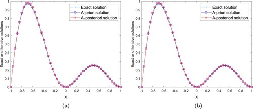
Figure 2. (a) $\alpha =0.008$. (b) $\alpha =0.02$. Example 4.1: $\beta =0.01$, $\epsilon =0.001$, $\gamma =0.9$, the exact and Landweber iterative solutions for $\alpha =0.008,0.02$.

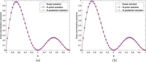
Figure 3. (a) $\beta =0.008$. (b) $\beta =0.02$. Example 4.1: $\alpha =0.01$, $\epsilon =0.001$, $\gamma =0.9$, the exact and Landweber iterative solutions for $\beta =0.008,0.02$.

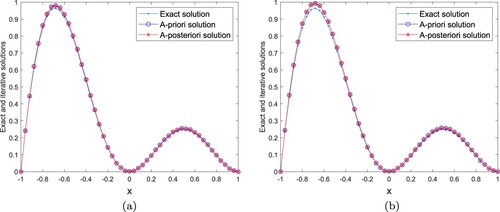
Table 1. Example 4.1: $\alpha =0.01$, $\beta =0.01$, $\gamma =0.9$, the relative errors for various noisy level ε.

ε	0.0001	0.0005	0.0007	0.005	0.01	0.05
$r_{pri}(u)$	0.0201	0.0199	0.0197	0.0174	0.0148	0.0181
$r_{post}(u)$	0.0200	0.0198	0.0197	0.0158	0.0133	0.0496

Table 2. Example 4.1: $\beta =0.01$, $\epsilon =0.001$, $\gamma =0.9$, the relative errors for various α.

α	0.008	0.01	0.02	0.03	0.04	0.05
$r_{pri}(u)$	0.0181	0.0196	0.0298	0.0401	0.0505	0.0611
$r_{post}(u)$	0.0180	0.0195	0.0296	0.0396	0.0496	0.0609

Table 3. Example 4.1: $\alpha =0.01$, $\epsilon =0.001$, $\gamma =0.9$, the relative errors for various β.

β	0.008	0.01	0.02	0.03	0.04	0.05
$r_{pri}(u)$	0.0175	0.0196	0.0298	0.0401	0.0505	0.0610
$r_{post}(u)$	0.0163	0.0195	0.0296	0.0396	0.0496	0.0609

Example 4.2

In the forward problem (40(40) $\begin{array}{r}\{\begin{array}{ll}{u}_t(x,t)-\alpha \mathrm{\Delta }u(x,t)+\beta (-\mathrm{\Delta }{)}^{\gamma }u(x,t)=\ell (x,t),& x\in \mathbb{R},t\in (0,T),\\ u(x,0)=h(x),& x\in \mathbb{R}.\end{array}\end{array}$(40) ), we take $\begin{array}{rl}h(x)& =\{\begin{array}{ll}0.5(-x+0.1{)}^2-0.125,& -0.4\le x\le 0.6,\\ 0,& \mathrm{others}.\end{array}\\ \ell (x,t)& =t\cdot \sin (x).\end{array}$we know that $h(x)$ is also a continuous function, and it only belongs to $H^1(\mathbb{R})\subset L^2(\mathbb{R})$. For the fixed $\alpha =0.01,\beta =0.01,\gamma =0.9$, Figure 4 shows the comparisons between the exact and regularized solutions for noise levels $\epsilon =0.0005,0.005$; the relative errors for various noisy level ε are presented in Table 4. For the fixed $\epsilon =0.005$, $\beta =0.01$, $\gamma =0.9$, the exact and regularization solutions are shown in Figure 5 with $\alpha =0.008$, 0.02; the relative errors for various α are listed in Table 5. Similar to the above situations, only β is changed, and other parameters remain unchanged, that is, $\alpha =0.01$, $\epsilon =0.005$, $\gamma =0.9$. In Figure 6, we show the comparisons between the exact and regularized solutions when $\beta =0.008$ and 0.02; the relative errors for various β are shown in Table 6.

Figure 4. (a) $\epsilon =0.0005$. (b) $\epsilon =0.005$. Example 4.2: $\alpha =0.01$, $\beta =0.01$, $\gamma =0.9$, the exact and Landweber iterative solutions for $\epsilon =0.0005,0.005$.

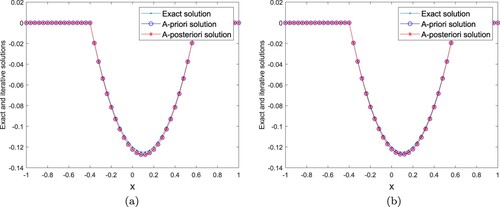
Figure 5. (a) $\alpha =0.008$. (b) $\alpha =0.02$. Example 4.2: $\beta =0.01$, $\epsilon =0.005$, $\gamma =0.9$, the exact and Landweber iterative solutions for $\alpha =0.008,0.02$.

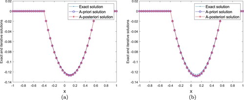
Figure 6. (a) $\beta =0.008$. (b) $\beta =0.02$. Example 4.2: $\alpha =0.01$, $\epsilon =0.005$, $\gamma =0.9$, the exact and Landweber iterative solutions for $\beta =0.008,0.02$.

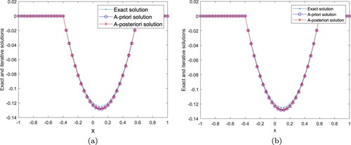
Table 4. Example 4.2: $\alpha =0.01$, $\beta =0.01$, $\gamma =0.9$, the relative errors for various noisy level ε.

ε	0.0001	0.0005	0.0007	0.005	0.01	0.05
$r_{pri}(u)$	0.0201	0.0198	0.0182	0.0171	0.0141	0.0148
$r_{post}(u)$	0.0200	0.0198	0.0197	0.0155	0.0125	0.0510

Table 5. Example 4.2: $\beta =0.01$, $\epsilon =0.005$, $\gamma =0.9$, the relative errors for various α.

α	0.008	0.01	0.02	0.03	0.04	0.1
$r_{pri}(u)$	0.0151	0.0171	0.0273	0.0376	0.0480	0.1127
$r_{post}(u)$	0.0138	0.0155	0.0238	0.0314	0.0471	0.1110

Table 6. Example 4.2: $\alpha =0.01$, $\epsilon =0.005$, $\gamma =0.9$, the relative errors for various β.

β	0.008	0.01	0.02	0.03	0.04	0.1
$r_{pri}(u)$	0.0151	0.0171	0.0273	0.0376	0.0480	0.1126
$r_{post}(u)$	0.0138	0.0155	0.0238	0.0314	0.0471	0.1110

Example 4.3

In the forward problem (40(40) $\begin{array}{r}\{\begin{array}{ll}{u}_t(x,t)-\alpha \mathrm{\Delta }u(x,t)+\beta (-\mathrm{\Delta }{)}^{\gamma }u(x,t)=\ell (x,t),& x\in \mathbb{R},t\in (0,T),\\ u(x,0)=h(x),& x\in \mathbb{R}.\end{array}\end{array}$(40) ), we take $h(x)=\{\begin{array}{ll}11(0.5+x),& -0.5\le x\le 0,\\ 11(0.5-x),& 0\le x\le 0.5,\\ 0,& \mathrm{others}.\end{array}$In [10], the authors used the spectral method to research a Riesz-Feller space fractional backward diffusion problem. Note that, when $\alpha =0$, $\beta =1$, $\ell (x,t)=0$, problem (1(1) $\begin{array}{r}\{\begin{array}{ll}{u}_t(x,t)-\alpha \mathrm{\Delta }u(x,t)+\beta (-\mathrm{\Delta }{)}^{\gamma }u(x,t)=\ell (x,t),& x\in \mathbb{R},t\in (0,T),\\ u(x,T)=\vartheta (x),& x\in \mathbb{R},\end{array}\end{array}$(1) ) becomes the following form (45) $\begin{array}{r}\{\begin{array}{ll}{u}_t(x,t)+(-\mathrm{\Delta }{)}^{\gamma }u(x,t)=0,& x\in \mathbb{R},t\in (0,T),\\ u(x,T)=\vartheta (x),& x\in \mathbb{R}.\end{array}\end{array}$(45) This is also a special case of Riesz-Feller space fractional backward diffusion problem in [10] as $\theta =0$. From [10], we know that the spectral regularization solution of (45(45) $\begin{array}{r}\{\begin{array}{ll}{u}_t(x,t)+(-\mathrm{\Delta }{)}^{\gamma }u(x,t)=0,& x\in \mathbb{R},t\in (0,T),\\ u(x,T)=\vartheta (x),& x\in \mathbb{R}.\end{array}\end{array}$(45) ) at t = 0 in the frequency domain can be written as (46) $\begin{array}{r}{\hat{u}}_s^{\delta }(\xi ,0)={\mathrm{e}}^{T|\xi {|}^{2\gamma }}{\hat{\vartheta }}^{\delta }\left(\xi \right){\chi }_{max},\end{array}$(46) where ${\chi }_{max}$ denotes the characteristic function of interval $[-{\xi }_{max},{\xi }_{max}]$, and ${\xi }_{max}=(\ln (\ln \frac{E}{\delta }){)}^{\frac{1}{2\gamma }}$ is chosen as the regularization parameter.

In addition, in [30], the authors proposed and used a fractional filter method to solve the inverse problem (1(1) $\begin{array}{r}\{\begin{array}{ll}{u}_t(x,t)-\alpha \mathrm{\Delta }u(x,t)+\beta (-\mathrm{\Delta }{)}^{\gamma }u(x,t)=\ell (x,t),& x\in \mathbb{R},t\in (0,T),\\ u(x,T)=\vartheta (x),& x\in \mathbb{R},\end{array}\end{array}$(1) ). According to [30], the regularization solution to problem (1(1) $\begin{array}{r}\{\begin{array}{ll}{u}_t(x,t)-\alpha \mathrm{\Delta }u(x,t)+\beta (-\mathrm{\Delta }{)}^{\gamma }u(x,t)=\ell (x,t),& x\in \mathbb{R},t\in (0,T),\\ u(x,T)=\vartheta (x),& x\in \mathbb{R},\end{array}\end{array}$(1) ) at t = 0 in frequency domain is defined as (47) $\begin{array}{r}\begin{array}{rl}{\hat{u}}_{\eta }^{\mu ,\delta }(\xi ,0)& =\frac{{\mathrm{e}}^{(\alpha |\xi {|}^2+\beta |\xi {|}^{2\gamma })T}}{1+\mu {(\alpha |\xi {|}^2+\beta |\xi {|}^{2\gamma })}^{\eta }{\mathrm{e}}^{(\alpha |\xi {|}^2+\beta |\xi {|}^{2\gamma })T}}\\ & \times (\widehat{{\vartheta }_{\delta }}(\xi )-{\int }_0^T{\mathrm{e}}^{(\alpha |\xi {|}^2+\beta |\xi {|}^{2\gamma })(\sigma -T)}{\hat{\ell }}_{\delta }(\xi ,\sigma )\mathrm{d}\sigma )\end{array}\end{array}$(47) where $\eta >1$, $\mu :=\mu (\delta )=\delta$ is the regularization parameter.

In this example, we do two numerical experiments. (I) we make some numerical comparisons between Landweber iterative method and the spectral method, here the spectral method is used to solve problem (45(45) $\begin{array}{r}\{\begin{array}{ll}{u}_t(x,t)+(-\mathrm{\Delta }{)}^{\gamma }u(x,t)=0,& x\in \mathbb{R},t\in (0,T),\\ u(x,T)=\vartheta (x),& x\in \mathbb{R}.\end{array}\end{array}$(45) ). (II) we make some numerical comparisons between Landweber iterative method and the fractional filter method in [30], and we take $\ell (x,t)=t\cdot \sin (x)$. In [10] and [30], the authors only considered the a-priori selection of regularization parameters, so we compare the numerical results under the a-prior selection of regularization parameters.

In experiment (I), we firstly take $\gamma =0.01$, Figures 7 and 8 are the comparison results between the exact solution, Landweber iterative solution and the spectral regularization solution for $\epsilon =0.0001$, $\epsilon =0.001$ respectively. The computer errors of two regularization solutions for various ε are listed in Table 7. Similarly, when $\epsilon =0.001$, $\gamma =0.001$ and $\gamma =0.01$, the comparison of two regular solutions and exact solution are listed in Figures 9–10. At the same time, through numerical verification, we find that γ has little impact on numerical results, so the error results are not listed.

Figure 7. (a) $\epsilon =0.0001$. (b) $\epsilon =0.001$. Example 4.3: Experiment (I), $\gamma =0.01$, the exact and Landweber iterative solutions for $\epsilon =0.0001,0.001$.

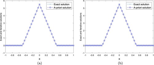
Figure 8. (a) $\epsilon =0.0001$. (b) $\epsilon =0.001$. Example 4.3: Experiment (I), $\gamma =0.01$, the exact and spectral regularization solutions for $\epsilon =0.0001,0.001$.

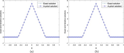
Figure 9. (a) $\gamma =0.001$. (b) $\gamma =0.01$. Example 4.3: Experiment (I), $\epsilon =0.001$, the exact and Landweber iterative solutions for $\gamma =0.001,0.01$.

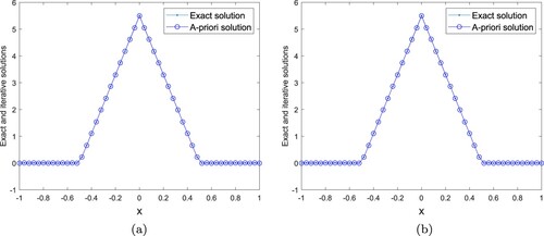
Figure 10. (a) $\gamma =0.001$. (b) $\gamma =0.01$. Example 4.3: Experiment (I), $\epsilon =0.001$, the exact and spectral regularization solutions for $\gamma =0.001,0.01$.

Table 7. Example 4.3: Experiment (I), $\gamma =0.01$, the relative errors for various ε.

ε	0.0001	0.0005	0.0007	0.001	0.005	0.09
$r_{pri}(u)$	$7.299\times {10}^{-4}$	$9.027\times {10}^{-4}$	$9.027\times {10}^{-4}$	0.0012	0.0037	0.0595
$r_{pri}(u_s^{\delta })$	$6.580\times {10}^{-5}$	$3.290\times {10}^{-4}$	$4.606\times {10}^{-4}$	$6.581\times {10}^{-4}$	0.0072	0.0592

In experiment (II), we fix $\alpha =0.01$, $\beta =0.01$, and $\gamma =0.9$, the comparison results between the exact solution, Landweber iterative solution and fractional filter method for $\epsilon =0.0001$ and $\epsilon =0.001$ are shown in Figures 11 and 12, respectively. For different ε, we show the relative errors in Table 8. For $\epsilon =0.001$, $\beta =0.01$ and $\gamma =0.9$, the numerical results of exact solution and two regularization solutions for $\alpha =0.008,0.02$ are shown in Figures 13 and 14. The relative errors for different α are listed in Table 9. In the same way, in Figures 15 and 16, we show the comparison results between the exact and regularized solutions as $\beta =0.008$, 0.02. The relative errors for various β are shown in Table 10.

Figure 11. (a) $\epsilon =0.0001$. (b) $\epsilon =0.001$. Example 4.3: Experiment (II), $\alpha =0.01$, $\beta =0.01$, $\gamma =0.9$, the exact and Landweber iterative solutions for $\epsilon =0.0001,0.001$.

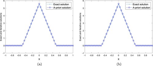
Figure 12. (a) $\epsilon =0.0001$. (b) $\epsilon =0.001$. Example 4.3: Experiment (II), $\alpha =0.01$, $\beta =0.01$, $\gamma =0.9$, the exact and fractional filter solutions for $\epsilon =0.0001,0.001$.

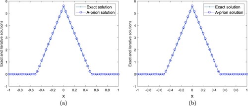
Figure 13. (a) $\alpha =0.008$. (b) $\alpha =0.02$. Example 4.3: Experiment (II), $\beta =0.01$, $\epsilon =0.001$, $\gamma =0.9$, the exact and Landweber iterative solutions for $\alpha =0.008,0.02$.

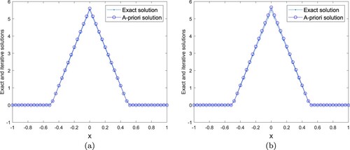
Figure 14. (a) $\alpha =0.008$. (b) $\alpha =0.02$. Example 4.3: Experiment (II), $\beta =0.01$, $\epsilon =0.001$, $\gamma =0.9$, the exact and fractional filter solutions for $\alpha =0.008,0.02$.

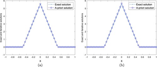
Figure 15. (a) $\beta =0.008$. (b) $\beta =0.02$. Example 4.3: Experiment (II), $\alpha =0.01$, $\epsilon =0.001$, $\gamma =0.9$, the exact and Landweber iterative solutions for $\beta =0.008,0.02$.

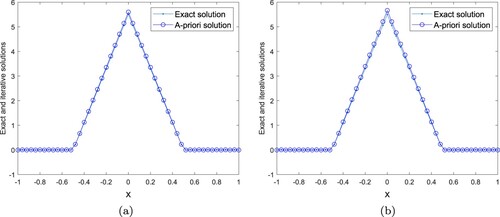
Figure 16. (a) $\beta =0.008$. (b) $\beta =0.02$. Example 4.3: Experiment (II), $\alpha =0.01$, $\epsilon =0.001$, $\gamma =0.9$, the exact and fractional filter solutions for $\beta =0.008,0.02$.

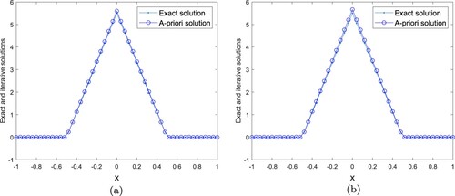
Table 8. Example 4.3: Experiment (II), $\alpha =0.01$, $\beta =0.01$, $\gamma =0.9$, the relative errors for various noisy level ε.

ε	0.0001	0.0005	0.0007	0.005	0.01	0.05
$r_{pri}(u)$	0.0201	0.0198	0.0197	0.0172	0.0143	0.0162
$r_{pri}(u_{\eta }^{\mu ,\delta })$	0.0201	0.0198	0.0197	0.0171	0.0143	0.0162

Table 9. Example 4.3: Experiment (II), $\beta =0.01$, $\epsilon =0.001$, $\gamma =0.9$, the relative errors for various α.

α	0.008	0.01	0.02	0.03	0.04	0.05
$r_{pri}(u)$	0.0175	0.0195	0.0298	0.0401	0.0505	0.0611
$r_{pri}(u_{\eta }^{\mu ,\delta })$	0.0175	0.0195	0.0298	0.0401	0.0504	0.0610

Table 10. Example 4.3: Experiment (II), $\alpha =0.01$, $\epsilon =0.001$, $\gamma =0.9$, the relative errors for various β.

β	0.008	0.01	0.02	0.03	0.04	0.05
$r_{pri}(u)$	0.0175	0.0195	0.0298	0.0401	0.0505	0.0610
$r_{pri}(u_{\eta }^{\mu ,\delta })$	0.0175	0.0195	0.0298	0.0401	0.0504	0.0610

From Figures 1–6 and Tables 1–6, we can see that numerical results are stable and satisfied when Landweber iteration method is used to solving the inverse initial value problem of diffusion equation with the local and nonlocal operators. Tables 1 and 4 indicate that, for the a-priori and a-posteriori cases, the computed error firstly decreases and then increases as ε becomes small. Tables 2 and 5 show that, for both a-priori and a-posteriori cases, the relative error becomes large with the increase of α. Tables 3 and 6 mean that, the smaller the parameter β is taken, the better numerical result becomes.

Figures 7–10 and Table 7 show that Landweber iterative method and spectral method are both feasible in solving problem (45(45) $\begin{array}{r}\{\begin{array}{ll}{u}_t(x,t)+(-\mathrm{\Delta }{)}^{\gamma }u(x,t)=0,& x\in \mathbb{R},t\in (0,T),\\ u(x,T)=\vartheta (x),& x\in \mathbb{R}.\end{array}\end{array}$(45) ). Meanwhile, we find that, for the small noise level ε, spectral method has better approximation effect than Landweber iterative method. However, as the noise level ε increases, the approximation effect of two methods is comparable. Figures 11–16 and Tables 8–10 mean that the simulation effect of Landweber iterative method and fractional filter method are equivalent in solving problem (1(1) $\begin{array}{r}\{\begin{array}{ll}{u}_t(x,t)-\alpha \mathrm{\Delta }u(x,t)+\beta (-\mathrm{\Delta }{)}^{\gamma }u(x,t)=\ell (x,t),& x\in \mathbb{R},t\in (0,T),\\ u(x,T)=\vartheta (x),& x\in \mathbb{R},\end{array}\end{array}$(1) ).

5. Conclusions

We consider an inverse initial value problem of diffusion equation with local and nonlocal operators. Firstly, we establish a result of conditional stability, and then use the Landweber iterative method to recover the stability of solution on measured datum. Meanwhile, the a-prior and a-posterior convergence estimates of Hölder type are derived, respectively. Finally, we make the corresponding verifications on the efficiency and accuracy of Landweber iterative method through numerical experiments. In the next works, we plan to study the inverse initial value problem of diffusion equation in which the diffusion operators are described by the coupling of local and Riesz-Feller space-fractional type.

Acknowledgments

The authors would like to thank the reviewers for their constructive comments and valuable suggestions that improve the quality of our paper.

Disclosure statement

No potential conflict of interest was reported by the author(s).

Additional information

Funding

The work was supported by the NSF of Ningxia (2022AAC03234), the NSF of China (11761004) and the Construction Project of First-Class Disciplines in Ningxia Higher Education (NXYLXK2017B09).

References

- Guo BL, Pu XK, Huang FH. Fractional partial differential equations and their numerical solutions. Singapore: World Scientific Publishing Company; 2015.
- Fu CL, Xiong XT, Qian Z. Fourier regularization for a backward heat equation. J Math Anal Appl. 2007;331(1):472–480.
- Hào DN, Duc NV. Stability results for the heat equation backward in time. J Math Anal Appl. 2008;353(2):627–641.
- Min T, Fu WM, Huang Q. Inverse estimates for nonhomogeneous backward heat problems. J Appl Math. 2014;2014(3):1 27Article ID 529618.
- Le TM, Pham QH, Luu PH. On an asymmetric backward heat problem with the space and time-dependent heat source on a disk. J Inverse Ill-Posed Probl. 2019;27(1):103–115.
- De SL, Song JT. Numerical method for solving nonhomogeneous backward heat conduction problem. Int J Differ Equ. 2018;2018:1–11.
- Arratia P, Coudurier M, Cueva E. Lipschitz stability for backward heat equation with application to fluorescence microscopy. SIAM J Math Anal. 2021;53(5):5948–5978.
- Ankita S, Mani M. Spectral graph wavelet regularization and adaptive wavelet for the backward heat conduction problem. Inverse Probl Sci Eng. 2021;29(4):457–488.
- Cheng W, Zhao Q. A modified quasi-boundary value method for a two-dimensional inverse heat conduction problem. Comput Math Appl. 2020;79(2):293–302.
- Zheng GH, Wei T. Two regularization methods for solving a Riesz-Feller space-fractional backward diffusion problem. Inverse Probl. 2010;26(11):Article ID 115017.
- Cheng H, Fu CL, Zheng GH, et al. A regularization for a Riesz-Feller space-fractional backward diffusion problem. Inverse Probl Sci Eng. 2014;22(6):860–872.
- Zhao JJ, Liu SS, Liu T. An inverse problem for space-fractional backward diffusion problem. Math Methods Appl Sci. 2014;37(8):1147–1158.
- Yang F, Li XX, Li DG, et al. The simplified Tikhonov regularization method for solving a Riesz-Feller space-fractional backward diffusion problem. Math Comput Sci. 2017;11(1):91–110.
- Zheng GH, Zhang QG. Recovering the initial distribution for space-fractional diffusion equation by a logarithmic regularization method. Appl Math Lett. 2016;61:143–148.
- Zheng GH, Zhang QG. Determining the initial distribution in space-fractional diffusion by a negative exponential regularization method. Inverse Probl Sci Eng. 2016;25(7):965–977.
- Zheng GH, Zhang QG. Solving the backward problem for space-fractional diffusion equation by a fractional Tikhonov regularization method. Math Comput Simul. 2018;148:37–47.
- Xiong XT, Wang JX, Li M. An optimal method for fractional heat conduction problem backward in time. Appl Anal. 2012;91(4):823–840.
- Zhang ZQ, Wei T. An optimal regularization method for space-fractional backward diffusion problem. Math Comput Simul. 2013;92:14–27.
- Liu CH, Mo ZW, Wu ZQ. Parameterization of vertical dispersion coefcient over idealized rough surfaces in isothermal conditions. Geosci Lett. 2018;5(1):1–11.
- Zhang HW, Zhang XJ. Solving the Riesz-Feller space-fractional backward diffusion problem by a generalized Tikhonov method. Adv Differ Equ. 2020;2020(1):376–384.
- Minh TL, Khieu TT, Khanh TQ, et al. On a space fractional backward diffusion problem and its approximation of local solution. J Comput Appl Math. 2019;346:440–455.
- Cassani D, Vilasi L, Wang YJ. Local versus nonlocal elliptic equations:short-long range field interactions. Adv Nonlinear Anal. 2021;10(1):895–921.
- LaMao CD, Huang SB, Tian QY, et al. Regularity results of solutions to elliptic equations involving mixed local and nonlocal operators. AIMS Math. 2022;7(3):4199–4210.
- dosSantos BC, Oliva SM, Rossi JD. Splitting methods and numerical approximations for a coupled local/nonlocal diffusion model. Comput Appl Math. 2021;41(1):6.
- Dipierro S, Lippi EP, Valdinoci E. (Non) local logistic equations with neumann conditions; 2021. arXiv:2101.02315.
- Slavova A, Popivanov P. Boundary value problems for local and nonlocal Liouville type equations with several exponential type nonlinearities. Radial and nonradial solutions. Adv Differ Equ. 2021;2021(1):386.
- Fang YZ, Shang B, Zhang C. Regularity theory for mixed local and nonlocal parabolic p-laplace equations. J Geom Anal. 2021;32(1):22.
- Mugnai D, Lippi EP. On mixed local-nonlocal operators with (α,β)-neumann conditions. Rend Circ Mat Palermo Ser 2. 2022;71(3):1035–1048.
- Biagi S, Dipierro S, Valdinoci E, et al. Mixed local and nonlocal elliptic operators: regularity and maximum principles. Commun Partial Differ Equ. 2022;47(3):585–629.
- Khieu TT, Khanh TQ. Fractional filter method for recovering the historical distribution for diffusion equations with coupling operator of local and nonlocal type. Numer Algorithms. 2022;89(4):1743–1767.
- Kirsch A. An introduction to the mathematical theory of inverse problems. New York: Springer; 2011.
- Engl HW, Hanke M, Neubauer A. Regularization of inverse problems. New York: Springer; 1996.
- Deng YJ, Liu ZH. Iteration methods on sideways parabolic equations. Inverse Probl. 2009;25(9):Article ID 095004.
- Vainikko GM, Veretennikov AY. Iteration procedures in ill-posed problems. Nauka: Moscow; 1986.
- Morozov VA, Nashed Z, Aries AB. Methods for solving incorrectly posed problems. New York: Springer; 1984.