A fractional-order model for computer viruses and some solution associated with residual power series method

Abstract

Awareness of virus spreading is an important issue for building various defence strategies and protecting personal computers, smart devices, network devices, etc. In this research work, we develop epidemiological models to address this problem and introduce certain modified epidemiological fractional SAIR model, where we consider the fractional derivative in Caputo sense. We utilize the residual power series method to construct approximate solutions for the governing system. To show the efficiency and suitability of the proposed technique, we introduce a comparative between the obtained solutions and those solutions that are constructed using the fourth-order Runge–Kutta method. We derive some numerical results by considering specific values for the parameters in the governing model, and then we depict some of these results into two and three dimensions.

Keywords:

• Fractional differential equations
• Caputo derivative
• absolute error
• epidemiological model
• computer viruses
• fractional epidemic model
• error function
• relative error

Mathematics Subject Classifications:

• 05A30
• 26D10
• 26D15
• 26A33
• Primary 54C40
• 14E20
• Secondary 46E25
• 20C20

1. Introduction

Fractional models are considered as a natural generalization to the classical models with integer order and receive a great attention in the scientific community due to their diverse applications in physics [1], astronomy [2], engineering [3], pharmacology [4] and medicine [5,6]. In literature, many local and non-local fractional operators have been developed and proposed including Caputo–Fabrizio [7], Riesz [8], Palmer [9], Letnikov [10], Grnwald [11], Riemann–Liouville [12], and AtanganaBaleanu operators [13]. This diversity depends on the nature of the real problem used in the applications [14,15].

The computer virus is a form of software that can replicate itself and spread to others from one computer. Viruses target the file system primarily, as worms use system weakness to scan and attack machines. However, computer viruses attacks are the major issues of the computer security and knowing their distribution is an essential component of any defensive strategy.

Since at least in 1988, several disease models discussing computer virus transmissions have been studied. Murray [16] is the first to propose the relationship between computer viruses and epidemiology. Even though Murray did not suggest particular models, he discussed analogies to certain epidemiological protection techniques for public health. A new model involving computer virus propagation on a multi-user device was studied by Gleissner [17], yet no provision was made for the identification and elimination to viruses. At recent days, a group has examined susceptible-infected-susceptible models for computer viruses dissemination at IBM Watson Research Center [18–21].

In recent years, researchers addressing different research questions about computer viruses aims to study computer viruses spreading models, propagation properties, control strategies, tipping point, and epidemic dynamics [22]. Researchers proposed different mathematical models that describe the computer viruses spreading. A number of these models use the general susceptible, infected, recovered (SIR) epidemic model. In Refs. [23,24], the authors applied the residual power series (RPS) method to analyse the SIR epidemic mode. They applied the technique to fractional SIR and compare the output results with the Runge–Kutta method. For computer epidemic, the SIR model is modified to include one more class of computers which are related to non-infected computers with anti-virus, the new model called SAIR. Therefore, computers in SAIR are classified into four classes: susceptible computers, non-infected computers with anti-virus, infected computers, and recovered computers [25]. Freihat et al. [26] used the multi-step homotopy analysis method to describe computer viruses spreading where the technique used is based on the SAIR model.

Furthermore, Lefebvre [27] focuses on the affection of the propagation of computer viruses and studies the time required to clean the infected computers. Furthermore, he divides computers into three categories: susceptible computers, infected computers, and recovered computers. The Lefebvre studies are based on the Kernack–McKendrick model which defines the dynamic of an infectious disease. Moreover, Kumar and Singh [28] proposed a new fractional epidemiological model with the use of Mittag–Lffler law to study the computer viruses spreading. Computer network, as a target of computer viruses, was studied by Upadhyay and Singh [29]. They classified computer nods in a network into two categories: the first category is called attacking class and the second is called targeted class. In each class, they define three types of computers based on the status of each computer: susceptible, infectious, and recovered. On the other side, Tang et al. [30] proposed a new network virus propagation model. The new type is called SLBRS which is based on states' cycle: susceptible, latent, breaking out, recovered, and susceptible. Other applications can be found in Refs. [31–36] and the references therein.

The mathematical model considered in this paper is based on dividing the computer into four groups, where T is the total number of computers. The criteria that have been adopted to classify the computer into groups are the computer status and the existence of the anti-virus. Hence, the four groups of computers are:

1. Susceptible (S): refers to non-infected computers by viruses but susceptible to be infected. These computers are a subject to be infected at any time according to a communication channel with infected computers.

2. Anti-virus (A): refers to non-infected computers by viruses but equipped with anti-virus.

3. Infected (I): refers to infected computers.

4. Removed (R): refers to removed computers due to an infection or not.

The total number of computers that are subject of this study is: $T=S+A+I+R$. The following non-linear system of first-order ordinary differential equations describes the SAIR model: (1) $\{\begin{array}{l}{\displaystyle \frac{\mathrm{d}S}{\mathrm{d}t}}=-{\alpha }_{SA}S(t)A(t)-\beta S(t)I(t)+\sigma R(t),\\ {\displaystyle \frac{\mathrm{d}A}{\mathrm{d}t}}={\alpha }_{SA}S(t)A(t)+{\alpha }_{IA}A(t)I(t),\\ {\displaystyle \frac{\mathrm{d}I}{\mathrm{d}t}}=\beta S(t)I(t)-{\alpha }_{IA}A(t)I(t)-\delta I(t),\\ {\displaystyle \frac{\mathrm{d}R}{\mathrm{d}t}}=\delta I(t)-\sigma R(t),\end{array}$(1) subject to $S(0)=S0,A(0)=A0,I(0)=I0,\mathrm{and}R(0)=R0.$Here, α, β, σ, and δ are positive constants. The rate of the susceptible computers S which supposed to be infected depends on creating a communication with infected computers. β is the rate of infections where the susceptible-infected computer communicates with infected ones since it is presented in the product SI. The conversion of the susceptible computers into secured computers (computers with anti-virus) is related to the product SA, as controlled by ${\alpha }_{SA}$, which depends on the foundation of anti-virus defined by computer administrator. On the other side, the use of anti-virus can fix the infected computers and convert them into secured computers with a rate related to AI with rate factor given by ${\alpha }_{IA}$. These computers are subject to be removed with the rate δ as they are being useless. Furthermore, there is a probability with rate σ to restore and convert the removed computer to susceptible computers. These scenarios are considered according to the assumption that the infection is related to known virus.

Based on previous scenarios, the definition of the SAIR model of fractional order can be written in the following form: (2) $\{\begin{array}{l}{\displaystyle \frac{1}{{\gamma }^{1-{\alpha }_1}}}{D}_0^{{\alpha }_1}S(t)=-{\alpha }_{SA}S(t)A(t)-\beta S(t)I(t)+\sigma R(t),\\ {\displaystyle \frac{1}{{\gamma }^{1-{\alpha }_2}}}{D}_0^{{\alpha }_2}A(t)={\alpha }_{SA}S(t)A(t)+{\alpha }_{IA}A(t)I(t),\\ {\displaystyle \frac{1}{{\gamma }^{1-{\alpha }_3}}}{D}_0^{{\alpha }_3}I(t)=\beta S(t)I(t)-{\alpha }_{IA}A(t)I(t)-\delta I(t),\\ {\displaystyle \frac{1}{{\gamma }^{1-{\alpha }_4}}}{D}_0^{{\alpha }_4}R(t)=\delta I(t)-\sigma R(t),\end{array}$(2) subject to (3) $S(0)=S_0,A(0)=A_0,I(0)=I_0,R(0)=R_0,$(3) where $D_0^{{\alpha }_1}S(t),D_0^{{\alpha }_2}A(t),D_0^{{\alpha }_3}I(t)$, and $D_0^{{\alpha }_4}R(t)$ are the Caputo derivatives of order ${\alpha }_1,{\alpha }_2,{\alpha }_3$, and ${\alpha }_4$ for $S(t),A(t),I(t)$, and $R(t)$, respectively, and $0<{\alpha }_j\le 1,i=1,2,3,4.$ To assure the match of the dimension in both sides in the fractional model (2), we consider the coefficient $1/{\gamma }^{1-{\alpha }_i}$ with aid of the auxiliary parameter γ [33]. The fractional model was considered here, because many physical phenomena have an substantial fractal order description, which makes it necessary to have a fractional system to explain such phenomena. Moreover, the fractional model provides a more accurate model than the ordinary calculus of physical systems [36–42]. We have considered the Caputo derivative in this work because it refers to the memory effect via a convolution between the integer order derivative and a power of time. This paper aims to utilize effective technique, the RPS method, and establish an approximate solution for the fractional SAIR model (1). The proposed method is easy to be performed and computationally attractive to gain the desired numerical solutions for the significant and notable governing model. Despite the importance of this system, it was not given enough attention to devise numerical solutions for it. So, the novelty of this paper lies in using the proposed method to provide such numerical solutions. We will also study the effect of the fractional derivative on the behaviour of the deduced solutions.

2. Preliminaries

The aim of this section is to present some of the fundamental meanings and facts of the fractional calculus and the fractional power series used in subsequent sections of this report.

Definition 2.1

A function $g(x)(x>0)$ is said to be in the space $C_{\beta }$ $(\beta \in \mathbb{R})$ if it can be written as $g(x)=x^p{g}_1(x)$ for some $p>\beta$ where $g_1(x)$ is continuous in $[0,\mathrm{\infty })$, and is said to be in the space $C_{\beta }^m$ if $g^{(m)}\in C_{\beta },m\in \mathbb{N}$.

Definition 2.2

The Riemann–Liouville integral operator of order β with $\beta \ge 0$ is defined as (4) $(J_a^{\beta }g)(x)=\frac{1}{\mathrm{\Gamma }(\beta )}{\int }_a^x(x-t{)}^{\beta -1}g(\xi )\mathrm{d}\xi ,x>a.$(4) The identity operator is $(J_a^{0}g)(x)$, for $\beta =0$. Hence, $(J_a^{0}g)(x)=g(x)$.

Definition 2.3

The Caputo fractional derivative of $g(x)$ of order $\beta >0$ with $a\ge 0$ is defined as (5) $(D_a^{\beta }g)(x)=(J_a^{m-\beta }{g}^{(m)})(x)=\frac{1}{\mathrm{\Gamma }(m-\beta )}{\int }_a^x\frac{g^{(m)}(\xi )}{(x-\xi {)}^{\beta +1-m}}\mathrm{d}\xi .$(5)

Definition 2.4

A power series expansion of the form (6) $\sum _{n=0}^{\mathrm{\infty }}{c}_n(t-t_0{)}^{na};0<\alpha \le 1,t_0\le t,$(6) is called a fractional power series about $t=t_0$. In particular, at $t_0=0$, the series $\sum _{n=0}^{\mathrm{\infty }}{c}_n(t{)}^{na}$ is said to be a fractional Maclaurin series. Furthermore, at $t=t_0$, with the understanding that the term corresponding to n = 0 in (9(9) $\{\begin{array}{l}{S}_n(t)=S_0+{\displaystyle \sum _{i=1}^n{\displaystyle \frac{a_i}{\mathrm{\Gamma }[1+i{\alpha }_1]}}{t}^{i{\alpha }_1},}\\ A_n(t)=A_0+{\displaystyle \sum _{i=1}^n{\displaystyle \frac{b_i}{\mathrm{\Gamma }[1+i{\alpha }_2]}}{t}^{i{\alpha }_2},}\\ I_n(t)=I_0+{\displaystyle \sum _{i=1}^n{\displaystyle \frac{c_i}{\mathrm{\Gamma }[1+i{\alpha }_3]}}{t}^{i{\alpha }_3},}\\ R_n(t)=R_0+{\displaystyle \sum _{i=1}^n{\displaystyle \frac{d_i}{\mathrm{\Gamma }[1+i{\alpha }_4]}}{t}^{i{\alpha }_4}.}\end{array}$(9) ), we consider the convention that $(t-t_0{)}^0=1$, whereas the fractional power series (9(9) $\{\begin{array}{l}{S}_n(t)=S_0+{\displaystyle \sum _{i=1}^n{\displaystyle \frac{a_i}{\mathrm{\Gamma }[1+i{\alpha }_1]}}{t}^{i{\alpha }_1},}\\ A_n(t)=A_0+{\displaystyle \sum _{i=1}^n{\displaystyle \frac{b_i}{\mathrm{\Gamma }[1+i{\alpha }_2]}}{t}^{i{\alpha }_2},}\\ I_n(t)=I_0+{\displaystyle \sum _{i=1}^n{\displaystyle \frac{c_i}{\mathrm{\Gamma }[1+i{\alpha }_3]}}{t}^{i{\alpha }_3},}\\ R_n(t)=R_0+{\displaystyle \sum _{i=1}^n{\displaystyle \frac{d_i}{\mathrm{\Gamma }[1+i{\alpha }_4]}}{t}^{i{\alpha }_4}.}\end{array}$(9) ) converges when $t=t_0$.

Theorem 2.5

Let f has a fractional power series (FPS) representation at $t=t_0$ of the form $f(t)=\sum _{m=0}^{\mathrm{\infty }}{c}_m(t-t_0{)}^{ma},$$t_0\le t<t_0+\varrho .$ It was found that when $D_{t_0}^{m\alpha }f(t),m=0,1,2,\dots$, are continuous on $(t_0,t_0+\varrho )$, then $c_m=D_{t_0}^{m}f(t_0)/\mathrm{\Gamma }(1+m\alpha )$ where Γ is the gamma function, $D_{t_0}^{m\alpha }=D_{t_0}^{\alpha }{D}_{t_0}^{\alpha }\dots D_{t_0}^{\alpha }$ (m-times), and ϱ is the radius of convergence.

3. RPS solution for SAIR of computer viruses

The solution of the non-linear fractional SAIR model is found by implementing the following steps:

Step1: This step has the initial assumption about $S(t),A(t),I(t)$, and $R(t)$ which have the FPS initial time $t_0=0$ as (7) $\{\begin{array}{l}S(t)={\displaystyle \sum _{i=0}^{\mathrm{\infty }}{\displaystyle \frac{a_i}{\mathrm{\Gamma }[1+i{\alpha }_1]}}{t}^{i{\alpha }_1},}\\ A(t)={\displaystyle \sum _{i=0}^{\mathrm{\infty }}{\displaystyle \frac{b_i}{\mathrm{\Gamma }[1+i{\alpha }_2]}}{t}^{i{\alpha }_2},}\\ I(t)={\displaystyle \sum _{i=0}^{\mathrm{\infty }}{\displaystyle \frac{c_i}{\mathrm{\Gamma }[1+i{\alpha }_3]}}{t}^{i{\alpha }_3},}\\ R(t)={\displaystyle \sum _{i=0}^{\mathrm{\infty }}{\displaystyle \frac{d_i}{\mathrm{\Gamma }[1+i{\alpha }_4]}}{t}^{i{\alpha }_4},}\end{array}$(7) where $0\le t<\varrho$ for some $\varrho >0$.

According to this assumption, we use the terms $S_n(t)$, $A_n(t)$, $I_n(t)$, and $(R_n(t)$ to denote the nth truncated series of $S(t),A(t),I(t),$ and $R(t)$, respectively, where they can be defined as (8) $\{\begin{array}{l}{S}_n(t)={\displaystyle \sum _{i=0}^n{\displaystyle \frac{a_i}{\mathrm{\Gamma }[1+i{\alpha }_1]}}{t}^{i{\alpha }_1},}\\ A_n(t)={\displaystyle \sum _{i=0}^n{\displaystyle \frac{b_i}{\mathrm{\Gamma }[1+i{\alpha }_2]}}{t}^{i{\alpha }_2},}\\ I_n(t)={\displaystyle \sum _{i=0}^n{\displaystyle \frac{c_i}{\mathrm{\Gamma }[1+i{\alpha }_3]}}{t}^{i{\alpha }_3},}\\ R_n(t)={\displaystyle \sum _{i=0}^n{\displaystyle \frac{d_i}{\mathrm{\Gamma }[1+i{\alpha }_4]}}{t}^{i{\alpha }_4}.}\end{array}$(8) From the initial condition in Equation (3(3) $S(0)=S_0,A(0)=A_0,I(0)=I_0,R(0)=R_0,$(3) ), where n = 0, we have $S_0(t)=a_0=S_0(0),A_0(t)=b_0=A_0(0)=A_0,I_0(0)=c_0=I_0(0)=I_0,$ and $R_0(t)=d_0=R_0(0)=R_0$. Thus, we can rewrite the nth truncated series in Equation (8(8) $\{\begin{array}{l}{S}_n(t)={\displaystyle \sum _{i=0}^n{\displaystyle \frac{a_i}{\mathrm{\Gamma }[1+i{\alpha }_1]}}{t}^{i{\alpha }_1},}\\ A_n(t)={\displaystyle \sum _{i=0}^n{\displaystyle \frac{b_i}{\mathrm{\Gamma }[1+i{\alpha }_2]}}{t}^{i{\alpha }_2},}\\ I_n(t)={\displaystyle \sum _{i=0}^n{\displaystyle \frac{c_i}{\mathrm{\Gamma }[1+i{\alpha }_3]}}{t}^{i{\alpha }_3},}\\ R_n(t)={\displaystyle \sum _{i=0}^n{\displaystyle \frac{d_i}{\mathrm{\Gamma }[1+i{\alpha }_4]}}{t}^{i{\alpha }_4}.}\end{array}$(8) ) in the following form: (9) $\{\begin{array}{l}{S}_n(t)=S_0+{\displaystyle \sum _{i=1}^n{\displaystyle \frac{a_i}{\mathrm{\Gamma }[1+i{\alpha }_1]}}{t}^{i{\alpha }_1},}\\ A_n(t)=A_0+{\displaystyle \sum _{i=1}^n{\displaystyle \frac{b_i}{\mathrm{\Gamma }[1+i{\alpha }_2]}}{t}^{i{\alpha }_2},}\\ I_n(t)=I_0+{\displaystyle \sum _{i=1}^n{\displaystyle \frac{c_i}{\mathrm{\Gamma }[1+i{\alpha }_3]}}{t}^{i{\alpha }_3},}\\ R_n(t)=R_0+{\displaystyle \sum _{i=1}^n{\displaystyle \frac{d_i}{\mathrm{\Gamma }[1+i{\alpha }_4]}}{t}^{i{\alpha }_4}.}\end{array}$(9) Step 2: The definition of the residual functions for the model is given in Equation (2(2) $\{\begin{array}{l}{\displaystyle \frac{1}{{\gamma }^{1-{\alpha }_1}}}{D}_0^{{\alpha }_1}S(t)=-{\alpha }_{SA}S(t)A(t)-\beta S(t)I(t)+\sigma R(t),\\ {\displaystyle \frac{1}{{\gamma }^{1-{\alpha }_2}}}{D}_0^{{\alpha }_2}A(t)={\alpha }_{SA}S(t)A(t)+{\alpha }_{IA}A(t)I(t),\\ {\displaystyle \frac{1}{{\gamma }^{1-{\alpha }_3}}}{D}_0^{{\alpha }_3}I(t)=\beta S(t)I(t)-{\alpha }_{IA}A(t)I(t)-\delta I(t),\\ {\displaystyle \frac{1}{{\gamma }^{1-{\alpha }_4}}}{D}_0^{{\alpha }_4}R(t)=\delta I(t)-\sigma R(t),\end{array}$(2) ): (10) $\{\begin{array}{l}Re{s}_S(t)=D_0^{{\alpha }_1}S(t)+{\alpha }_{SA}S(t)A(t)+\beta S(t)I(t)-\sigma R(t),\\ Re{s}_A(t)=D_0^{{\alpha }_2}A(t)-{\alpha }_{SA}S(t)A(t)-{\alpha }_{IA}A(t)I(t),\\ Re{s}_I(t)=D_0^{{\alpha }_3}I(t)-\beta S(t)I(t)+{\alpha }_{IA}A(t)I(t)+\delta I(t),\\ Re{s}_R(t)=D_0^{{\alpha }_4}R(t)-\delta I(t)+\sigma R(t).\end{array}$(10) Therefore, the definition of the nth residual functions of $S(t),A(t),I(t),$ and $R(t)$ are, respectively, (11) $\{\begin{array}{l}Re{s}_{S,n}(t)=D_0^{{\alpha }_1}{S}_n(t)+{\alpha }_{SA}{S}_n(t)A_n(t)+\beta S_n(t)I_n(t)-\sigma R_n(t),\\ Re{s}_{A,n}(t)=D_0^{{\alpha }_2}{A}_n(t)-{\alpha }_{SA}{S}_n(t)A_n(t)-{\alpha }_{IA}{A}_n(t)I_n(t),\\ Re{s}_{I,n}(t)=D_0^{{\alpha }_3}{I}_n(t)-\beta S_n(t)I_n(t)+{\alpha }_{IA}{A}_n(t)I_n(t)+\delta I_n(t),\\ Re{s}_{R,n}(t)=D_0^{{\alpha }_4}{R}_n(t)-\delta I_n(t)+\sigma R_n(t).\end{array}$(11) Obviously, $\begin{array}{rl}& Re{s}_S(t)=Re{s}_A(t)=Re{s}_I(t)=Re{s}_R(t)=0\mathrm{\forall }t\ge 0,\underset{n\to \mathrm{\infty }}{lim}Re{s}_{S,n}(t)=Re{s}_S(t),\\ & \underset{n\to \mathrm{\infty }}{lim}Re{s}_{A,n}(t)=Re{s}_A(t),\underset{n\to \mathrm{\infty }}{lim}Re{s}_{I,n}(t)=Re{s}_I(t),\mathrm{and}\underset{n\to \mathrm{\infty }}{lim}Re{s}_{R,n}(t)=Re{s}_R(t).\end{array}$From the fact that the Caputo derivative of any constant is zero, we can conclude that [37] $\begin{array}{rl}& D_0^{(i-1){\alpha }_1}Re{s}_S(0)=D_0^{(i-1){\alpha }_1}Re{s}_{S,i}(0),D_0^{(i-1){\alpha }_2}Re{s}_A(0)=D_0^{(i-1){\alpha }_2}Re{s}_{A,i}(0),\\ & D_0^{(i-1){\alpha }_3}Re{s}_I(0)=D_0^{(i-1){\alpha }_3}Re{s}_{I,i}(0),D_0^{(i-1){\alpha }_4}Re{s}_R(0)=D_0^{(i-1){\alpha }_4}Re{s}_{R,i}(0)\\ & \mathrm{for}i=1,\dots ,n.\end{array}$The following steps based on this main idea are considered in the core of the RPS method.

Step 3: In this step, the nth truncated series of $S(t),A(t),I(t),$ and $R(t)$ are substituted into Equation (11(11) $\{\begin{array}{l}Re{s}_{S,n}(t)=D_0^{{\alpha }_1}{S}_n(t)+{\alpha }_{SA}{S}_n(t)A_n(t)+\beta S_n(t)I_n(t)-\sigma R_n(t),\\ Re{s}_{A,n}(t)=D_0^{{\alpha }_2}{A}_n(t)-{\alpha }_{SA}{S}_n(t)A_n(t)-{\alpha }_{IA}{A}_n(t)I_n(t),\\ Re{s}_{I,n}(t)=D_0^{{\alpha }_3}{I}_n(t)-\beta S_n(t)I_n(t)+{\alpha }_{IA}{A}_n(t)I_n(t)+\delta I_n(t),\\ Re{s}_{R,n}(t)=D_0^{{\alpha }_4}{R}_n(t)-\delta I_n(t)+\sigma R_n(t).\end{array}$(11) ) to obtain the coefficients $a_i,b_i,c_i,$ and $d_i$, where $i=0,1,2,3,\dots ,n$. Then, the Caputo fractional derivative operators $D_0^{(n-1){\alpha }_1},D_0^{(n-1){\alpha }_2}$, $D_0^{(n-1){\alpha }_3}$, and $D_0^{(n-1){\alpha }_4}$ are applied on $Re{s}_{S,n}(0)=0,Re{s}_{A,n}(0)=0,Re{s}_{I,n}(0)=0,$ and $Re{s}_{R,n}(0)=0$, respectively. The following equations are the desired result: (12) $\{\begin{array}{l}{D}_0^{(n-1){\alpha }_1}Re{s}_{S,n}(0)=0\\ D_0^{(n-1){\alpha }_2}Re{s}_{A,n}(0)=0\\ D_0^{(n-1){\alpha }_3}Re{s}_{I,n}(0)=0\\ D_0^{(n-1){\alpha }_4}Re{s}_{R,n}(0)=0\end{array}forn=1,2,3,\dots .$(12)

4. Implementation and numerical results

For the accuracy of the FRPSM against the known built-in fourth-order Runge–Kutta (RK4), Mathematica procedure will be demonstrated for computer viruses in the case of the integer order derivatives. The FRPSM is coded in Mathematica 10 computer algebra kit. In all calculations performed in this article, Mathematica environment variable digits, which regulate the sum of the significant digits, are set to 20. The fractional SAIR model subject to $S(0)=3,A(0)=1,I(0)=95$, and $R(0)=1$ is (13) $\{\begin{array}{l}{D}_0^{\alpha }S(t)=-0.025S(t)A(t)-0.1S(t)I(t)+0.8R(t),\\ D_0^{\alpha }A(t)=0.025S(t)A(t)+0.25A(t)I(t),\\ D_0^{\alpha }I(t)=0.1S(t)I(t)-0.25A(t)I(t)-9I(t),\\ D_0^{\alpha }R(t)=9I(t)-0.8R(t).\end{array}$(13) We refer to the order of the fractional derivative by α where it is in the range $0<\alpha \le 1$. Using the RPS method's steps, which was discussed in Section 3, leads to the following forms of the first truncated power series approximations $\begin{array}{rl}{S}_1(t)& =3+\frac{a_1}{\mathrm{\Gamma }(1+\alpha )}{t}^{\alpha },\\ A_1(t)& =1+\frac{b_1}{\mathrm{\Gamma }(1+\alpha )}{t}^{\alpha },\\ I_1(t)& =95+\frac{c_1}{\mathrm{\Gamma }(1+\alpha )}{t}^{\alpha },\\ R_1(t)& =1+\frac{d_1}{\mathrm{\Gamma }(1+\alpha )}{t}^{\alpha }.\end{array}$Based on Equation (11(11) $\{\begin{array}{l}Re{s}_{S,n}(t)=D_0^{{\alpha }_1}{S}_n(t)+{\alpha }_{SA}{S}_n(t)A_n(t)+\beta S_n(t)I_n(t)-\sigma R_n(t),\\ Re{s}_{A,n}(t)=D_0^{{\alpha }_2}{A}_n(t)-{\alpha }_{SA}{S}_n(t)A_n(t)-{\alpha }_{IA}{A}_n(t)I_n(t),\\ Re{s}_{I,n}(t)=D_0^{{\alpha }_3}{I}_n(t)-\beta S_n(t)I_n(t)+{\alpha }_{IA}{A}_n(t)I_n(t)+\delta I_n(t),\\ Re{s}_{R,n}(t)=D_0^{{\alpha }_4}{R}_n(t)-\delta I_n(t)+\sigma R_n(t).\end{array}$(11) ), the first residual functions of $S(t)$, $A(t)$, $I(t)$, and $R(t)$ are, respectively, given as follows: $\begin{array}{rl}Re{s}_{S,1}(t)& =D_0^{\alpha }(3+\frac{a_1}{\mathrm{\Gamma }(1+\alpha )}{t}^{\alpha })+0.025(3+\frac{a_1}{\mathrm{\Gamma }(1+\alpha )}{t}^{\alpha })(1+\frac{b_1}{\mathrm{\Gamma }(1+\alpha )}{t}^{\alpha })\\ & +0.1(3+\frac{a_1}{\mathrm{\Gamma }(1+\alpha )}{t}^{\alpha })(95+\frac{c_1}{\mathrm{\Gamma }(1+\alpha )}{t}^{\alpha })-0.8(1+\frac{d_1}{\mathrm{\Gamma }(1+\alpha )}{t}^{\alpha })\\ & =27.775+a_1+\frac{9.525t^{\alpha }{a}_1}{\mathrm{\Gamma }(1+\alpha )}+\frac{0.075t^{\alpha }{b}_1}{\mathrm{\Gamma }(1+\alpha )}+\frac{0.025t^{2\alpha }{a}_1{b}_1}{\mathrm{\Gamma }(1+\alpha {)}^2}+\frac{0.3t^{\alpha }{c}_1}{\mathrm{\Gamma }(1+\alpha )}\\ & +\frac{0.1t_{2\alpha }{a}_1{c}_1}{\mathrm{\Gamma }(1+\alpha {)}^2}+\frac{0.8t^{\alpha }{d}_1}{\mathrm{\Gamma }(1+\alpha )},\\ Re{s}_{A,1}(t)& =D_0^{\alpha }(1+\frac{b_1}{\mathrm{\Gamma }(1+\alpha )}{t}^{\alpha })-0.025(3+\frac{a_1}{\mathrm{\Gamma }(1+\alpha )}{t}^{\alpha })(1+\frac{b_1}{\mathrm{\Gamma }(1+\alpha )}{t}^{\alpha })\\ & -0.25(1+\frac{b_1}{\mathrm{\Gamma }(1+\alpha )}{t}^{\alpha })(95+\frac{c_1}{\mathrm{\Gamma }(1+\alpha )}{t}^{\alpha })\\ & =-23.825-\frac{0.025t^{\alpha }{a}_1}{\mathrm{\Gamma }(1+\alpha )}+b_1-\frac{23.825t^{\alpha }{b}_1}{\mathrm{\Gamma }(1+\alpha )}-\frac{0.025t^{2\alpha }{a}_1{b}_1}{\mathrm{\Gamma }(1+\alpha {)}^2}-\frac{0.25t^{\alpha }{c}_1}{\mathrm{\Gamma }(a+\alpha )}\\ & -\frac{0.25t^{2\alpha }{b}_1{c}_1}{\mathrm{\Gamma }(1+\alpha {)}^2},\\ Re{s}_{I,1}(t)& =D_0^{\alpha }(95+\frac{c_1}{\mathrm{\Gamma }(1+\alpha )}{t}^{\alpha })-0.1(3+\frac{a_1}{\mathrm{\Gamma }(1+\alpha )}{t}^{\alpha })(95+\frac{c_1}{\mathrm{\Gamma }(1+\alpha )}{t}^{\alpha })\\ & +0.25(1+\frac{b_1}{\mathrm{\Gamma }(1+\alpha )}{t}^{\alpha })(95+\frac{c_1}{\mathrm{\Gamma }(1+\alpha )}{t}^{\alpha })+9(95+\frac{c_1}{\mathrm{\Gamma }(1+\alpha )}{t}^{\alpha })\\ & =850.25-\frac{9.5t^{\alpha }{a}_1}{\mathrm{\Gamma }(1+\alpha )}+\frac{23.75t^{\alpha }{b}_1}{\mathrm{\Gamma }(1+\alpha )}+c_1+\frac{8.95t^{\alpha }{c}_1}{\mathrm{\Gamma }(1+\alpha )}-\frac{0.1t^{2\alpha }{a}_1{c}_1}{\mathrm{\Gamma }(1+\alpha {)}^2}\\ & +\frac{0.25t^{2\alpha }{b}_1{c}_1}{\mathrm{\Gamma }(1+\alpha {)}^2},\\ Re{s}_{R,1}(t)& =D_0^{{\alpha }_4}(1+\frac{d_1}{\mathrm{\Gamma }(1+\alpha )}{t}^{\alpha })-9(95+\frac{c_1}{\mathrm{\Gamma }(1+\alpha )}{t}^{\alpha })+0.8(1+\frac{d_1}{\mathrm{\Gamma }(1+\alpha )}{t}^{\alpha })\\ & =-854.2-\frac{9t^{\alpha }{c}_1}{\mathrm{\Gamma }(1+\alpha )}+d_1+\frac{0.8t^{\alpha }{d}_1}{\mathrm{\Gamma }(1+\alpha )}.\end{array}$We can compute the value of $a_1$, $b_1$, $c_1$, and $d_1$ by equating $Re{s}_{S,1}(0)$, $Re{s}_{A,1}(0)$, $Re{s}_{I,1}(0)$, and $Re{s}_{R,1}(0)$ by zero. Hence, $\begin{array}{rl}{S}_1(t)& =3-\frac{27.775t^{\alpha }}{\mathrm{\Gamma }(1+\alpha )},\\ A_1(t)& =1+\frac{23.825t^{\alpha }}{\mathrm{\Gamma }(1+\alpha )},\\ I_1(t)& =95-\frac{850.25t^{\alpha }}{\mathrm{\Gamma }(1+\alpha )},\\ R_1(t)& =1+\frac{854.2t^{\alpha }}{\mathrm{\Gamma }(1+\alpha )}.\end{array}$For n = 2, the forms for the second truncated power series approximation are $\begin{array}{rl}{S}_2(t)& =3-\frac{27.775t^{\alpha }}{\mathrm{\Gamma }(1+\alpha )}+\frac{t^{2\alpha }{a}_2}{\mathrm{\Gamma }(1+2\alpha )},\\ A_2(t)& =1+\frac{23.825t^{\alpha }}{\mathrm{\Gamma }(1+\alpha )}+\frac{t^{2\alpha }{b}_2}{\mathrm{\Gamma }(1+2\alpha )},\\ I_2(t)& =95-\frac{850.25t^{\alpha }}{\mathrm{\Gamma }(1+\alpha )},+\frac{t^{2\alpha }{c}_2}{\mathrm{\Gamma }(1+2\alpha )},\\ R_2(t)& =1+\frac{854.2t^{\alpha }}{\mathrm{\Gamma }(1+\alpha )}+\frac{t^{2\alpha }{d}_2}{\mathrm{\Gamma }(1+2\alpha )}.\end{array}$Hence, the second residual functions are $\begin{array}{rl}Re{s}_{S,2}(t)& =D_0^{\alpha }(3-\frac{27.775t^{\alpha }}{\mathrm{\Gamma }(1+\alpha )}+\frac{t^{2\alpha }{a}_2}{\mathrm{\Gamma }(1+2\alpha )})+0.025(3-\frac{27.775t^{\alpha }}{\mathrm{\Gamma }(1+\alpha )}+\frac{t^{2\alpha }{a}_2}{\mathrm{\Gamma }(1+2\alpha )})\\ & \times (1+\frac{23.825t^{\alpha }}{\mathrm{\Gamma }(1+\alpha )}+\frac{t^{2\alpha }{b}_2}{\mathrm{\Gamma }(1+2\alpha )})\\ & +0.1(3-\frac{27.775t^{\alpha }}{\mathrm{\Gamma }(1+\alpha )}+\frac{t^{2\alpha }{a}_2}{\mathrm{\Gamma }(1+2\alpha )})(95-\frac{850.25t^{\alpha }}{\mathrm{\Gamma }(1+\alpha )},+\frac{t^{2\alpha }{c}_2}{\mathrm{\Gamma }(1+2\alpha )})\\ & -0.8(1+\frac{854.2t^{\alpha }}{\mathrm{\Gamma }(1+\alpha )}+\frac{t^{2\alpha }{d}_2}{\mathrm{\Gamma }(1+2\alpha )}),\\ Re{s}_{A,2}(t)& =D_0^{\alpha }(1+\frac{23.825t^{\alpha }}{\mathrm{\Gamma }(1+\alpha )}+\frac{t^{2\alpha }{b}_2}{\mathrm{\Gamma }(1+2\alpha )})-0.025(3-\frac{27.775t^{\alpha }}{\mathrm{\Gamma }(1+\alpha )}+\frac{t^{2\alpha }{a}_2}{\mathrm{\Gamma }(1+2\alpha )})\\ & \times (1+\frac{23.825t^{\alpha }}{\mathrm{\Gamma }(1+\alpha )}+\frac{t^{2\alpha }{b}_2}{\mathrm{\Gamma }(1+2\alpha )})\\ & -0.25(1+\frac{23.825t^{\alpha }}{\mathrm{\Gamma }(1+\alpha )}+\frac{t^{2\alpha }{b}_2}{\mathrm{\Gamma }(1+2\alpha )})(95-\frac{850.25t^{\alpha }}{\mathrm{\Gamma }(1+\alpha )},+\frac{t^{2\alpha }{c}_2}{\mathrm{\Gamma }(1+2\alpha )}),\\ Re{s}_{I,2}(t)& =D_0^{\alpha }(95-\frac{850.25t^{\alpha }}{\mathrm{\Gamma }(1+\alpha )},+\frac{t^{2\alpha }{c}_2}{\mathrm{\Gamma }(1+2\alpha )})-0.1(3-\frac{27.775t^{\alpha }}{\mathrm{\Gamma }(1+\alpha )}+\frac{t^{2\alpha }{a}_2}{\mathrm{\Gamma }(1+2\alpha )})\\ & \times (95-\frac{850.25t^{\alpha }}{\mathrm{\Gamma }(1+\alpha )},+\frac{t^{2\alpha }{c}_2}{\mathrm{\Gamma }(1+2\alpha )})\\ & +0.25(1+\frac{23.825t^{\alpha }}{\mathrm{\Gamma }(1+\alpha )}+\frac{t^{2\alpha }{b}_2}{\mathrm{\Gamma }(1+2\alpha )})(95-\frac{850.25t^{\alpha }}{\mathrm{\Gamma }(1+\alpha )},+\frac{t^{2\alpha }{c}_2}{\mathrm{\Gamma }(1+2\alpha )})\\ & +9(95-\frac{850.25t^{\alpha }}{\mathrm{\Gamma }(1+\alpha )},+\frac{t^{2\alpha }{c}_2}{\mathrm{\Gamma }(1+2\alpha )}),\\ Re{s}_{R,2}(t)& =D_0^{\alpha }(1+\frac{854.2t^{\alpha }}{\mathrm{\Gamma }(1+\alpha )}+\frac{t^{2\alpha }{d}_2}{\mathrm{\Gamma }(1+2\alpha )})-9(95-\frac{850.25t^{\alpha }}{\mathrm{\Gamma }(1+\alpha )},+\frac{t^{2\alpha }{c}_2}{\mathrm{\Gamma }(1+2\alpha )})\\ & +0.8(1+\frac{854.2t^{\alpha }}{\mathrm{\Gamma }(1+\alpha )}+\frac{t^{2\alpha }{d}_2}{\mathrm{\Gamma }(1+2\alpha )}).\end{array}$Applying the operator $D_0^{\alpha }$ to $Re{s}_{S,2}(t)$, $Re{s}_{A,2}(t)$, $Re{s}_{I,2}(t)$, and $Re{s}_{R,2}(t)$ yields $\begin{array}{rl}{D}_0^{\alpha }Re{s}_{S,2}(t)& =\frac{4690.051781t^{\alpha }\alpha \mathrm{\Gamma }[2\alpha ]}{\mathrm{\Gamma }[1+\alpha {]}^3}-\frac{1201.205\alpha \mathrm{\Gamma }[\alpha ]}{\mathrm{\Gamma }[1+\alpha ]}+\frac{1.0\alpha \mathrm{\Gamma }[\alpha ]a_2}{\mathrm{\Gamma }[1+\alpha ]}\\ & -\frac{253.2881250t^{2\alpha }\alpha \mathrm{\Gamma }[3\alpha ]a_2}{\mathrm{\Gamma }[1+\alpha ]\mathrm{\Gamma }[1+2\alpha {]}^2}+\frac{19.05t^{\alpha }\alpha \mathrm{\Gamma }[2\alpha ]a_2}{\mathrm{\Gamma }[1+\alpha ]\mathrm{\Gamma }[1+2\alpha ]}\\ & -\frac{2.083125t^{2\alpha }\alpha \mathrm{\Gamma }[3\alpha ]b_2}{\mathrm{\Gamma }[1+\alpha ]\mathrm{\Gamma }[1+2\alpha {]}^2}+\frac{0.15t^{\alpha }\alpha \mathrm{\Gamma }[2\alpha ]b_2}{\mathrm{\Gamma }[1+\alpha ]\mathrm{\Gamma }[1+2\alpha ]}\\ & +\frac{0.1t^{3\alpha }\alpha \mathrm{\Gamma }[4\alpha ]a_2{b}_2}{\mathrm{\Gamma }[1+2\alpha {]}^2\mathrm{\Gamma }[1+3\alpha ]}-\frac{8.3325t^{2\alpha }\alpha \mathrm{\Gamma }[3\alpha ]c_2}{\mathrm{\Gamma }[1+\alpha ]\mathrm{\Gamma }[1+2\alpha {]}^2}\\ & +\frac{0.6t^{\alpha }\alpha \mathrm{\Gamma }[2\alpha ]c_2}{\mathrm{\Gamma }[1+\alpha ]\mathrm{\Gamma }[1+2\alpha ]}+\frac{0.4t^{3\alpha }\alpha \mathrm{\Gamma }[4\alpha ]a_2{c}_2}{\mathrm{\Gamma }[1+2\alpha {]}^2\mathrm{\Gamma }[1+3\alpha ]}\\ & -\frac{1.6t^{\alpha }\alpha \mathrm{\Gamma }[2\alpha ]d_2}{\mathrm{\Gamma }[1+\alpha ]\mathrm{\Gamma }[1+2\alpha ]},\\ D_0^{\alpha }Re{s}_{A,2}(t)& =\frac{10161.69009t^{\alpha }\alpha \mathrm{\Gamma }[2\alpha ]}{\mathrm{\Gamma }[1+\alpha {]}^3}-\frac{354.37375\alpha \mathrm{\Gamma }[\alpha ]}{\mathrm{\Gamma }[1+\alpha ]}-\frac{1.786875t^{2\alpha }\alpha \mathrm{\Gamma }[3\alpha ]a_2}{\mathrm{\Gamma }[1+\alpha ]\mathrm{\Gamma }[1+2\alpha {]}^2}\\ & -\frac{0.05t^{\alpha }\alpha \mathrm{\Gamma }[2\alpha ]a_2}{\mathrm{\Gamma }[1+\alpha ]\mathrm{\Gamma }[1+2\alpha ]}+\frac{1.0\alpha \mathrm{\Gamma }[\alpha ]b_2}{\mathrm{\Gamma }[1+\alpha ]}\\ & +\frac{639.770625t^{2\alpha }\alpha \mathrm{\Gamma }[3\alpha ]b_2}{\mathrm{\Gamma }[1+\alpha ]\mathrm{\Gamma }[1+2\alpha {]}^2}-\frac{47.65t^{\alpha }\alpha \mathrm{\Gamma }[2\alpha ]b_2}{\mathrm{\Gamma }[1+\alpha ]\mathrm{\Gamma }[1+2\alpha ]}-\frac{0.1t^{3\alpha }\alpha \mathrm{\Gamma }[4\alpha ]a_2{b}_2}{\mathrm{\Gamma }[1+2\alpha {]}^2\mathrm{\Gamma }[1+3\alpha ]}\\ & -\frac{17.86875t^{2\alpha }\alpha \mathrm{\Gamma }[3\alpha ]c_2}{\mathrm{\Gamma }[1+\alpha ]\mathrm{\Gamma }[1+2\alpha {]}^2}-\frac{0.5t^{\alpha }\alpha \mathrm{\Gamma }[2\alpha ]c_2}{\mathrm{\Gamma }[1+\alpha ]\mathrm{\Gamma }[1+2\alpha ]}\\ & -\frac{1.0t^{3\alpha }\alpha \mathrm{\Gamma }[4\alpha ]b_2{c}_2}{\mathrm{\Gamma }[1+2\alpha {]}^2\mathrm{\Gamma }[1+3\alpha ]},\\ D_0^{\alpha }Re{s}_{I,2}(t)& =-\frac{14851.74188t^{\alpha }\alpha \mathrm{\Gamma }[2\alpha ]}{\mathrm{\Gamma }[1+\alpha {]}^3}-\frac{6780.03125\alpha \mathrm{\Gamma }[\alpha ]}{\mathrm{\Gamma }[1+\alpha ]}+\frac{255.075t^{2\alpha }\alpha \mathrm{\Gamma }[3\alpha ]a_2}{\mathrm{\Gamma }[1+\alpha ]\mathrm{\Gamma }[1+2\alpha {]}^2}\\ & -\frac{19.0t^{\alpha }\alpha \mathrm{\Gamma }[2\alpha ]a_2}{\mathrm{\Gamma }[1+\alpha ]\mathrm{\Gamma }[1+2\alpha ]}-\frac{637.6875t^{2\alpha }\alpha \mathrm{\Gamma }[3\alpha ]b_2}{\mathrm{\Gamma }[1+\alpha ]\mathrm{\Gamma }[1+2\alpha {]}^2}\\ & +\frac{47.5t^{\alpha }\alpha \mathrm{\Gamma }[2\alpha ]b_2}{\mathrm{\Gamma }[1+\alpha ]\mathrm{\Gamma }[1+2\alpha ]}+\frac{1.0\alpha \mathrm{\Gamma }[\alpha ]c_2}{\mathrm{\Gamma }[1+\alpha ]}+\frac{26.20125t^{2\alpha }\alpha \mathrm{\Gamma }[3\alpha ]c_2}{\mathrm{\Gamma }[1+\alpha ]\mathrm{\Gamma }[1+2\alpha {]}^2}\\ & +\frac{17.9t^{\alpha }\alpha \mathrm{\Gamma }[2\alpha ]c_2}{\mathrm{\Gamma }[1+\alpha ]\mathrm{\Gamma }[1+2\alpha ]}-\frac{0.4t^{3\alpha }\alpha \mathrm{\Gamma }[4\alpha ]a_2{c}_2}{\mathrm{\Gamma }[1+2\alpha {]}^2\mathrm{\Gamma }[1+3\alpha ]}+\frac{1.0t^{3\alpha }\alpha \mathrm{\Gamma }[4\alpha ]b_2{c}_2}{\mathrm{\Gamma }[1+2\alpha {]}^2\mathrm{\Gamma }[1+3\alpha ]},\\ D_0^{\alpha }Re{s}_{R,2}(t)& =\frac{8335.61\alpha \mathrm{\Gamma }[\alpha ]}{\mathrm{\Gamma }[1+\alpha ]}-\frac{18.0t^{\alpha }\alpha \mathrm{\Gamma }[2\alpha ]c_2}{\mathrm{\Gamma }[1+\alpha ]\mathrm{\Gamma }[1+2\alpha ]}+\frac{1.0\alpha \mathrm{\Gamma }[\alpha ]d_2}{\mathrm{\Gamma }[1+\alpha ]}\\ & +\frac{1.6t^{\alpha }\alpha \mathrm{\Gamma }[2\alpha ]d_2}{\mathrm{\Gamma }[1+\alpha ]\mathrm{\Gamma }[1+2\alpha ]}.\end{array}$The value of $a_0$, $b_0$, $c_0$, and $d_0$ can be computed using the fact $D_0^{\alpha }Re{s}_{S,2}(0)=D_0^{\alpha }Re{s}_{A,2}(0)=D_0^{\alpha }Re{s}_{I,2}(0)=D_0^{\alpha }Re{s}_{R,2}(0)=0.$Therefore, we have $\begin{array}{rl}{S}_2(t)& =3-\frac{27.775t^{\alpha }}{\mathrm{\Gamma }(1+\alpha )}+\frac{1201.205t^{2\alpha }{a}_2}{\mathrm{\Gamma }(1+2\alpha )},\\ A_2(t)& =1+\frac{23.825t^{\alpha }}{\mathrm{\Gamma }(1+\alpha )}+\frac{\mathrm{354.37.75}{t}^{2\alpha }{b}_2}{\mathrm{\Gamma }(1+2\alpha )},\\ I_2(t)& =95-\frac{850.25t^{\alpha }}{\mathrm{\Gamma }(1+\alpha )}+\frac{6780.03125t^{2\alpha }{c}_2}{\mathrm{\Gamma }(1+2\alpha )},\\ R_2(t)& =1+\frac{854.2t^{\alpha }}{\mathrm{\Gamma }(1+\alpha )}+\frac{8335.61t^{2\alpha }{d}_2}{\mathrm{\Gamma }(1+2\alpha )}.\end{array}$Continuing this process, we get the third approximations $\begin{array}{rl}{S}_3(t)& =3-\frac{27.775t^{\alpha }}{\mathrm{\Gamma }[1+\alpha ]}+\frac{1201.205t^{2\alpha }}{\mathrm{\Gamma }[1+2\alpha ]}\\ & +\left[\frac{\begin{array}{c}0.5t^{3\alpha }\mathrm{\Gamma }[1.0+\alpha ](-(4690.052{\alpha }^2\mathrm{\Gamma }[\alpha ]\mathrm{\Gamma }[2.0\alpha ]/\mathrm{\Gamma }[1.0+\alpha {]}^3)\\ -(40341.11{\alpha }^2\mathrm{\Gamma }[\alpha ]\mathrm{\Gamma }[2.0\alpha ]/\mathrm{\Gamma }[1.0+\alpha ]\mathrm{\Gamma }[1.0+2.0\alpha ]))\mathrm{\Gamma }[1.0+2.0\alpha ]\end{array}}{{\alpha }^2\mathrm{\Gamma }[\alpha ]\mathrm{\Gamma }[2.0\alpha ]\mathrm{\Gamma }[1+3\alpha ]}\right],\\ A_3(t)& =1+\frac{23.825t^{\alpha }}{\mathrm{\Gamma }[1+\alpha ]}+\frac{354.37375t^{2\alpha }}{\mathrm{\Gamma }[1+2\alpha ]}\\ & -\left[\frac{t^{3\alpha }{\alpha }^2\mathrm{\Gamma }[\alpha ]\mathrm{\Gamma }[2.0\alpha ](10161.690-(20335.99\mathrm{\Gamma }[1.0+\alpha {]}^2/\mathrm{\Gamma }[1.0+2.0\alpha ]))}{\mathrm{\Gamma }[1.0+\alpha {]}^3\mathrm{\Gamma }[1+3\alpha ]}\right],\\ I_3(t)& =95-\frac{850.25t^{\alpha }}{\mathrm{\Gamma }[1+\alpha ]}+\frac{6780.031t^{2\alpha }}{\mathrm{\Gamma }[1+2\alpha ]}\\ & -\left[\frac{t^{3\alpha }{\alpha }^2\mathrm{\Gamma }[\alpha ]\mathrm{\Gamma }[2.0\alpha ](-14851.74+(115372.4\mathrm{\Gamma }[1.0+\alpha {]}^2/\mathrm{\Gamma }[1.0+2.0\alpha ]))}{\mathrm{\Gamma }[1.0+\alpha {]}^3\mathrm{\Gamma }[1+3\alpha ]}\right],\\ R_3(t)& =1+\frac{854.2t^{\alpha }}{\mathrm{\Gamma }[1+\alpha ]}-\frac{8335.61t^{2\alpha }}{\mathrm{\Gamma }[1+2\alpha ]}+\frac{67688.8t^{3\alpha }}{\mathrm{\Gamma }[1+3\alpha ]}.\end{array}$Tables 1–4 represent a numerical comparison between RK4 solution and RPS solution for $\alpha =1$. The results show the accuracy of RPS for approximating the solution of the SAIR model. Furthermore, the absolute error $Ab{s}_S(t_i)$ and relative error $Re{l}_S(t_i)$ are computed for $S(t)$ as shown in Table 1, where the $Ab{s}_S(t_i)$ as an absolute error is defined in Equations (14(14) $\begin{array}{rl}Ab{s}_S(t_i)& =|\mathrm{RK}{4}_S(t_i)-{\mathrm{RPS}}_S(t_i)|\end{array}$(14) ) and (15(15) $\begin{array}{rl}Re{l}_S(t_i)& =\left|\frac{\mathrm{RK}{4}_S(t_i)-{\mathrm{RPS}}_S(t_i)}{\mathrm{RK}{4}_S(t_i)}\right|\mathrm{\forall }i=0,1,2,\dots ,10.\end{array}$(15) ) and shows the definition of the relative error. Tables 2– 4 show the absolute value and the relative value of $A(t)$, $I(t)$, and $R(t)$, respectively. (14) $\begin{array}{rl}Ab{s}_S(t_i)& =|\mathrm{RK}{4}_S(t_i)-{\mathrm{RPS}}_S(t_i)|\end{array}$(14) (15) $\begin{array}{rl}Re{l}_S(t_i)& =\left|\frac{\mathrm{RK}{4}_S(t_i)-{\mathrm{RPS}}_S(t_i)}{\mathrm{RK}{4}_S(t_i)}\right|\mathrm{\forall }i=0,1,2,\dots ,10.\end{array}$(15) From the observed results in Tables 1–4, we conclude that by using few approximations to obtain a high accuracy via RPS technique. Moreover, from the use of the independent values of the interval [0,1], we observe that the estimated error is more accurate. Finally, the results that show a higher accuracy are achieved as more components of RPS solution are evaluated. Overall, the tables represent that there is a high effectiveness of using the RPS technique.

Figures 1–4 show comparison between the RK and RPS solution of $S(t)$, $A(t)$, $I(t)$, and $R(t)$ for $\alpha =1$.

Figure 1. Comparison between the RK and RPS solution of $S(t)$.

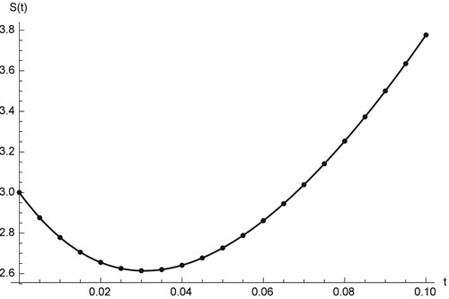
Table 1. Approximate solution of $S(t)$ using RK4 and RPS methods.

t	$\mathrm{RK}S(t_i),\alpha =1$	$\mathrm{RPS}S(t_i),\alpha =1$	$Ab{s}_S(t_i)$	$Re{l}_S(t_i)$
0	3	3	0	0
0.01	2.77843	2.77843	${3.22464}^{-9}$	${1.1606}^{-9}$
0.02	2.65554	2.65554	${9.27018}^{-10}$	${3.49089}^{-10}$
0.03	2.61433	2.61433	${1.99140}^{-9}$	${7.61725}^{-10}$
0.04	2.64152	2.64152	${1.94573}^{-10}$	${7.36593}^{-11}$
0.05	2.72662	2.72662	${2.26315}^{-10}$	${8.30022}^{-11}$
0.06	2.86124	2.86124	${8.17013}^{-11}$	${2.85545}^{-11}$
0.07	3.03862	3.03862	${5.86511}^{-10}$	${1.93019}^{-10}$
0.08	3.25322	3.25322	${1.84048}^{-8}$	${5.65741}^{-9}$
0.09	3.50048	3.50048	${2.34799}^{-7}$	${6.70762}^{-8}$
0.1	3.77656	3.77656	${2.16865}^{-6}$	${5.74239}^{-7}$

Table 2. Approximate solution of $A(t)$ using RK4 and RPS methods.

t	$\mathrm{RK}A(t_i),\alpha =1$	$\mathrm{RPS}A(t_i),\alpha =1$	$Ab{s}_A(t_i)$	$Re{l}_A(t_i)$
0	1	1	0	0
0.01	1.25592	1.25592	${1.13764}^{-9}$	${9.05819}^{-10}$
0.02	1.54662	1.54662	${3.47133}^{-9}$	${2.24446}^{-9}$
0.03	1.87043	1.87043	${5.33983}^{-9}$	${2.85487}^{-9}$
0.04	2.22465	2.22465	${8.69501}^{-9}$	${3.90849}^{-9}$
0.05	2.60573	2.60573	${1.17096}^{-8}$	${4.49377}^{-9}$
0.06	3.00947	3.00947	${1.51163}^{-8}$	${5.02291}^{-9}$
0.07	3.43118	3.43118	${1.89419}^{-8}$	${5.52053}^{-9}$
0.08	3.86597	3.86597	${2.27410}^{-8}$	${5.88235}^{-9}$
0.09	4.30892	4.30892	${1.74213}^{-8}$	${4.04308}^{-9}$
0.1	4.75527	4.75527	${6.68440}^{-8}$	${1.40568}^{-8}$

Table 3. Approximate solution of $I(t)$ using RK4 and RPS methods.

t	$\mathrm{RK}I(t_i),\alpha =1$	$\mathrm{RPS}I(t_i),\alpha =1$	$Ab{s}_I(t_i)$	$Re{l}_I(t_i)$
0	95	95	0	0
0.01	86.8293	86.8293	${1.71273}^{-9}$	${1.97253}^{-11}$
0.02	79.2936	79.2936	${3.65712}^{-9}$	${4.61212}^{-11}$
0.03	72.3505	72.3505	${4.85059}^{-9}$	${6.7043}^{-11}$
0.04	65.9589	65.9589	${9.42981}^{-9}$	${1.42965}^{-10}$
0.05	60.0801	60.0801	${1.25570}^{-8}$	${2.09005}^{-10}$
0.06	54.6776	54.6776	${1.53807}^{-8}$	${2.81297}^{-10}$
0.07	49.7173	49.7173	${1.61516}^{-8}$	${3.24869}^{-10}$
0.08	45.1675	45.1675	${6.92892}^{-9}$	${1.53405}^{-10}$
0.09	40.9984	40.9984	${2.91477}^{-7}$	${7.10946}^{-9}$
0.1	37.1826	37.1826	${2.88429}^{-6}$	${7.75709}^{-8}$

Table 4. Approximate solution of $R(t)$ using RK4 and RPS methods.

t	$\mathrm{RK}I(t_i),\alpha =1$	$\mathrm{RPS}I(t_i),\alpha =1$	$Ab{s}_I(t_i)$	$Re{l}_I(t_i)$
0	1	1	0	0
0.01	9.13632	9.13632	${2.64954}^{-9}$	${2.90001}^{-10}$
0.02	16.5042	16.5042	${7.41228}^{-10}$	${4.49115}^{-11}$
0.03	23.1648	23.1648	${2.48064}^{-9}$	${1.07087}^{-10}$
0.04	29.1749	29.1749	${9.29361}^{-10}$	${3.18548}^{-11}$
0.05	34.5875	34.5875	${1.07384}^{-9}$	${3.10469}^{-11}$
0.06	39.4517	39.4517	${1.82688}^{-10}$	${4.63067}^{-12}$
0.07	43.8129	43.8129	${2.20384}^{-9}$	${5.03012}^{-11}$
0.08	47.7133	47.7133	${1.12651}^{-8}$	${2.361}^{-10}$
0.09	51.1922	51.1922	${7.40994}^{-8}$	${1.44747}^{-9}$
0.1	54.2856	54.2856	${6.48794}^{-7}$	${1.19515}^{-8}$

Figures 1–4 show the comparison between the RPS and the RK4 solution, where the fractional order is $\alpha =1$ and the sample size is k = 20. From the chart in figures, we see that the approximation which results from using the RPS methods is efficient and can be achieved by implementing similar technique on small samples as in our case is only 20. Figures 1–4 show that the two methods can be obtained on $S(t),A(t),I(t)$, and $R(t)$ and can predict the behaviour of the four compartments accurately.

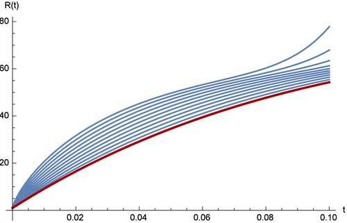
Figures 5–8 show the RPS solution of $S(t)$, $A(t)$, $I(t)$, and $R(t)$ for different value of α. In Figures 5–8, the RPS approximation methods for the four computer categories (susceptible, anti-virus, infected, and recovered) are established for different values of α. The sub-figures show the graphical line for the different values of ${\alpha }_j=0.1j$, where $j=1,2,3,\dots ,10$ with step s = 0.02 over the interval [0,0.1]. In the figures, it is clear that the degree of the freedom for the fractional order derivation is greater than the degree of the integer order derivation. From the four curves of $S(t),A(t),I(t)$, and $R(t)$, we can observe that the four curves of the fractional SAIR model are close to the classical SAIR model as the fractional order close to the integer order.

Figure 2. Comparison between the RK and RPS solution of $A(t)$.

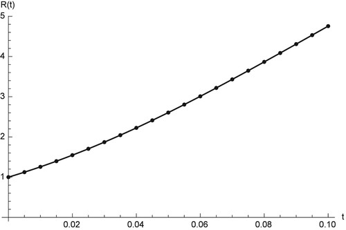
Figure 3. Comparison between the RK and RPS solution of $I(t)$.

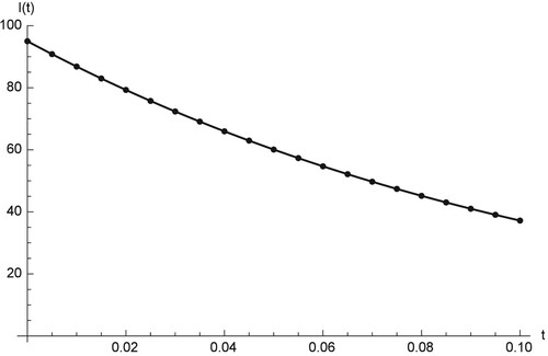
Figure 4. Comparison between the RK and RPS solution of $R(t)$.

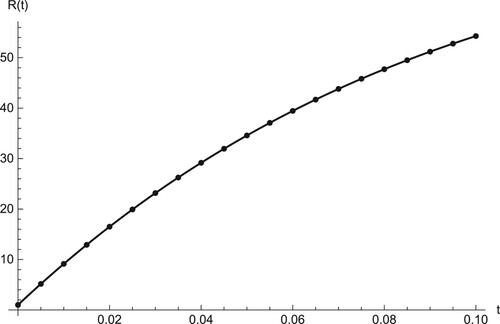
Figure 5. The RPS solution of $S(t)$ for different values of α.

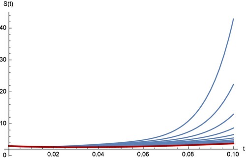
Figure 6. The RPS solution of $A(t)$ for different values of α.

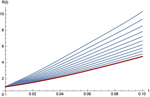
Figure 7. The RPS solution of $I(t)$ for different values of α.

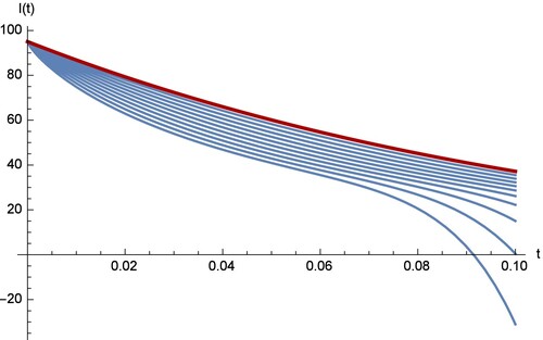
Figure 8. The RPS solution of $R(t)$ for different values of α.

5. Conclusion

In this paper, we deal with significant model in computer science, SAIR model, which provides a perception of the problem of viruses in the computer field. The fractional version of the SAIR model was considered in this paper. We utilize the power full tool, RPS method, to construct an approximate solution to the governing model. Some of the obtained results have been depicted in two and three dimensions to illustrate the physical properties of it at the selected values for the considered parameters. Moreover, we compare the developed approximate solutions using Runge–Kutta method. The analytical approach solutions of the model are shown to be accurate and have a long time validity. It should be noted that there are very few works in the literature that provide approximate solutions to the governing system in this paper. Therefore, the novelty of this paper lies in presenting approximate solutions to this fractional system using new simple and easy-to-apply method to discuss and study the governing system. The RPSM's power and the capacity are also provided as an easy tool for computing non-linear problem solutions that appear as models in some fields including certain models in science and engineering topics.

Acknowledgments

This research has received funding support from the National Science, Research and Innovation Fund (NSRF), Thailand.

Disclosure statement

No potential conflict of interest was reported by the authors.

Additional information

Funding

This paper have not received any funding in any form.

References

- Kumar S. A new fractional modeling arising in engineering sciences and its analytical approximate solution. Alex Eng J. 2013;52(4):813–819.
- Kilbas A, Srivastava H, Trujillo J. Theory and applications of fractional differential equations. Amsterdam: Elsevier; 2006.
- Al-Smadi M, Djeddi N, Momani S, et al. An attractive numerical algorithm for solving nonlinear Caputo–Fabrizio fractional Abel differential equation in a Hilbert space. Adv Differ Equ. 2021;2021(1):271.
- Al-Smadi M, Abu Arqub O, Zeidan D. Fuzzy fractional differential equations under the Mittag–Leffler kernel differential operator of the ABC approach: theorems and applications. Chaos Solitons Fractals. 2021;146:Article ID 110891.
- Al-Smadi M. Simplified iterative reproducing kernel method for handling time-fractional BVPs with error estimation. Ain Shams Eng J. 2018;9(4):2517–2525.
- Hasan S, Al-Smadi M, El-Ajou A, et al. Numerical approach in the Hilbert space to solve a fuzzy Atangana–Baleanu fractional hybrid system. Chaos Solitons Fractals. 2021;143:Article ID 110506.
- Abuteen E, Freihat A, Al-Smadi M, et al. Approximate series solution of nonlinear, fractional Klein–Gordon equations using fractional reduced differential transform method. J Math Stat. 2016;12(1):23–33.
- Al-Smadi M, Freihat A, Khalil H, et al. Numerical multistep approach for solving fractional partial differential equations. Int J Comput Methods. 2021;14(3):Article ID 1750029.
- Moaddy K, Freihat A, Al-Smadi M, et al. Numerical investigation for handling fractional-order Rabinovich–Fabrikant model using the multistep approach. Soft Comput. 2018;22(3):773–782.
- Al-Smadi M, Abu Arqub O. Computational algorithm for solving Fredholm time-fractional partial integrodifferential equations of Dirichlet functions type with error estimates. Appl Math Comput. 2019;342:280–294.
- Al-Smadi M, Freihat A, Abu Hammad M, et al. Analytical approximations of partial differential equations of fractional order with multistep approach. J Comput Theor Nanosci. 2016;13(11):7793–7801.
- Alabedalhadi M, Al-Smadi M, Al-Omari S, et al. Structure of optical soliton solution for nonlinear resonant space–time Schrdinger equation in conformable sense with full nonlinearity term. Phys Scr. 2020;95(10):Article ID 105215.
- Al-Smadi M, Dutta H, Hasan S, et al. On numerical approximation of Atangana–Baleanu–Caputo fractional integro-differential equations under uncertainty in Hilbert space. Math Model Nat Phenom. 2021;16:41.
- Al-Smadi M, Abu Arqub O, Hadid S. An attractive analytical technique for coupled system of fractional partial differential equations in shallow water waves with conformable derivative. Commun Theor Phys. 2020;72(8):Article ID 085001.
- Al-Smadi M, Abu Arqub O, Hadid S. Approximate solutions of nonlinear fractional Kundu–Eckhaus and coupled fractional massive Thirring equations emerging in quantum field theory using conformable residual power series method. Phys Scr. 2020;95(10):Article ID 105205.
- Murray W. The application of epidemiology to computer viruses. Comput Secur. 1988;7(2):139–145.
- Gleissner W. A mathematical theory for the spread of computer viruses. Comput Secur. 1989;8(1):35–41.
- Kephart JO, White SR. Directed-graph epidemiological models of computer viruses. In: Proceedings of the IEEE symposium on security and privacy, USA; 1991. p. 343–359.
- Kephart JO, White SR. Measuring and modelling computer virus prevalence. In: Proceedings of the IEEE symposium on security and privacy; 1993. p. 2–15.
- Kephart JO, White SR, Chess DM. Computers and epidemiology. J Mag. 1993;5:20–26.
- Kephart JO, Sorkin GB, Chess DM, et al. Fighting computer viruses. Sci Am. 1997;277:88–93.
- Huang CY, Lee CL, Wen TH, et al. A computer virus spreading model based on resource limitations and interaction costs. J Syst Softw. 2013;86(3):801–808.
- Hasan S, Al-Zoubi A, Freihet A, et al. Solution of fractional SIR epidemic model using residual power series method. Appl Math Inf Sci. 2019;13(2):153–161.
- Freihat AA, Handam AH. Solution of the SIR models of epidemics using MSGDTM. Appl Appl Math. 2014;9(2):622–636.
- Piqueira JRC, Araujo VO. A modified epidemiological model for computer viruses. Appl Math Comput. 2009;213(2):355–360.
- Freihat A, Zurigat M, Handam A. The multi-step homotopy analysis method for modified epidemiological model for computer viruses. Afr Mat. 2015;26(3–4):585–596.
- Lefebvre M. A stochastic model for computer virus propagation. J Dyn Games. 2020;7(2):163.
- Kumar D, Singh J. New aspects of fractional epidemiological model for computer viruses with Mittag–Leffler law. Math Model Health Soc Appl Sci. 2020;39:283–301.
- Upadhyay RK, Singh P. Modeling and control of computer virus attack on a targeted network. Phys A: Stat Mech Appl. 2020;538:Article ID 122617.
- Tang W, Liu Y-J, Chen Y-L, et al. SLBRS: network virus propagation model based on safety entropy. Appl Soft Comput. 2020;97:Article ID 106784.
- Al-Smadi M, Abu Arqub O, Momani S. A computational method for two-point boundary value problems of fourth-order mixed integrodifferential equations. Math Probl Eng. 2013;2013:Article ID 832074.
- Han X, Tan Q. Dynamical behavior of computer virus on internet. Appl Math Comput. 2010;217(6):2520–2526.
- Baleanu D, Abadi M, Jajarmi A, et al. A new comparative study on the general fractional model of COVID-19 with isolation and quarantine effects. Alex Eng J. 2022;61(6):4779–4791.
- Baleanu D, Ghassabzade F, Nieto J, et al. On a new and generalized fractional model for a real cholera outbreak. Alex Eng J. 2022;61(11):9175–9186.
- Erturk V, Godwe E, Baleanu D, et al. Novel fractional-order Lagrangian to describe motion of beam on nanowire. Acta Phys Pol. 2022;140(3):265–272.
- Agarwal P, Nieto J, Ruzhansky M, et al. Analysis of infectious disease problems (Covid-19) and their global impact. Singapore: Springer; 2021.
- El-Ajou A, Abu Arqub O, Al-Smadi M. A general form of the generalized Taylors formula with some applications. Appl Math Comput. 2015;256:851–859.
- Kumar S, Ahmadian A, Kumar R, et al. An efficient numerical method for fractional SIR epidemic model of infectious disease by using Bernstein wavelets. Mathematics. 2020;8(4):558.
- Farman M, Ahmad A, Akgl A, et al. Epidemiological analysis of the coronavirus disease outbreak with random effects. Comput Mater Contin. 2021;67(3):3215–3227.
- Komashynska I, Al-Smadi M, Abu Arqub O, et al. An efficient analytical method for solving singular initial value problems of nonlinear systems. Appl Math Inf Sci. 2016;10(2):647–656.
- Al-Smadi M, Abu Arqub O, El-Ajou A. A numerical iterative method for solving systems of first-order periodic boundary value problems. J Appl Math. 2014;2014:Article ID 135465.
- Chen J, Hu M-B, Li M. Traffic-driven epidemic spreading in multiplex networks. Phys Rev E. 2020;101:Article ID 012301.
- Al-Jarrah A, Massa'deh MO, Baareh AEK, et al. A study on r-edge regular intuitionistic fuzzy graphs. J Math Comput Sci. 2021;23(4):279–288.