A generalized study of the distribution of buffer over calcium on a fractional dimension

Abstract

Calcium is an essential element in our body and plays a vital role in moderating calcium signalling. Calcium is also called the second messenger. Calcium signalling depends on cytosolic calcium concentration. In this study, we focus on cellular calcium fluctuations with different buffers, including calcium-binding buffers, using the Hilfer fractional advection-diffusion equation for cellular calcium. Limits and start conditions are also set. By combining with intracellular free calcium ions, buffers reduce the cytosolic calcium concentration. The buffer depletes cellular calcium and protects against toxicity. Association, dissociation, diffusion, and buffer concentration are modelled. The solution of the Hilfer fractional calcium model is achieved through utilizing the integral transform technique. To investigate the influence of the buffer on the calcium concentration distribution, simulations are done in MATLAB 21. The results show that the modified calcium model is a function of time, position, and the Hilfer fractional derivative. Thus the modified Hilfer calcium model provides a richer physical explanation than the classical calcium model.

Keywords:

• Buffer
• calcium concentration
• Hilfer fractional derivative
• Laplace transform
• Fourier transform

MSC:

• 26A33
• 35Q92
• 44A10
• 92C99

1. Introduction

Calcium is required for almost every process in the human body, such as heartbeat, muscle contraction, cell cycle, fate, metabolism, bone movement, brain function, etc. Calcium performs various vascular procedures such as information processing and blood flow. Calcium is also known as the second messenger and is found in almost all nerve cells, such as neurons, astrocytes, hepatocytes, and many others. Although calcium is essential for the sustenance of life, its increased concentration spells death; therefore, it is necessary to maintain the calcium intake.

In practically all types of human and animal cells, calcium signalling is a fundamental component of cell communication. This calcium signalling controls all vital functions of the hepatocyte cell, which is a parenchymal cell of the liver. The concentration of cytosolic calcium affects calcium signalling. A prerequisite for the proper functioning of the calcium messenger system in higher organisms is maintaining the concentration of cytosolic calcium in the resting cell deficient. Calcium signalling in excitatory and non-excitable cells is dependent on relatively low cytosolic calcium concentrations and the existence of a calcium concentration gradient existing among the cytosol and the passage of intracellular organelles.

After being released from the calcium channel gate in the cytoplasm, $\text{C}{a}^{+2}$ ions undergo various physical processes such as transport, buffering, etc. Calcium transport occurs in the cytoplasm by a combination of convection and diffusion. The buffering mechanism also controls the calcium concentration. In the cytoplasm, approximately 99$\mathrm{\%}$ of calcium binds with the buffer to alter the enzymatic characteristics of calcium [1]. Calcium-binding buffers serve an essential function in lowering intracellular calcium concentrations by binding to free $\text{C}{a}^{+2}$ ions. The equilibrium between the 'on' and 'off' response, which brings Ca into the cytoplasm, consequently the 'off' reaction, so it removes the signal through the joint action of exchangers, pumps, and buffers determines the intracellular calcium level at any given moment.

Buffers are defined as solutions that resist changes in pH by the addition of a small amount of acid or base. That is, it maintains the pH of the body. In this paper, we study about protein buffer system. Protein in the human form is made up of amino acids with functional groups that act as the acid of the week and base to stabilize the pH within the body's cell.

In this paper, we have discussed four buffers (EGTA, Troponine, Calmodulin, BAPTA). BAPTA primarily protects cells against toxic calcium overload. EGTA is a chelating agent with a high affinity for calcium ions. EGTA is used as a buffer equal to the pH of the living cell. Calmodulin is a critical neuronal protein that is a crucial mediator of several $\text{C}{a}^{+2}$-dependent intracellular signalling cascades in the brain. Calmodulin modulates synaptic transmission and synaptic plasticity through Ca, which relies on its target proteins in pre and postsynaptic compartments. Calmodulin is a regulatory protein used to detect changes in calcium ion concentration.

Many real-world issues have been solved through mathematical modelling [2–4]. Many mathematical models have been proposed to describe the common phenomena of intracellular and intercellular calcium oscillations. This paper used an analytical technique to tackle the one-dimensional issue of calcium diffusion. Previous research includes studies by Meyer et al. [5] conducted experimental investigations with favourable findings, obtaining results utilizing molecular modelling for the receptor of calcium profiles. Nehar [6] investigated linearized buffered Ca diffusion in the microdomain. Winston et al. [7] constructed a model to explain intracellular calcium fluctuations in endothelium cells. Smith et al. [8] used a circularly symmetric area to describe the occurrence above to determine the rapid buffering approximation near an open calcium channel. Agarwal et al. [9] investigated the influence such as the fractional advection-diffusion equation, on the calcium concentration characteristics. Several theoretical studies have also been conducted in recent decades. Jha et al. [10] utilized an FVM to examine the influence of buffer on cytosolic Ca. A model to describe the calcium distribution in neuron cells has been proposed by Tripathi et al. [11]. Agarwal et al. [12] used a fractional model to investigate the buffer over cytosol calcium concentration distribution.

Signaling depends on how calcium impacts $\text{C}{a}^{+2}$ mobility in cells. We've discussed buffers' influence on intracellular calcium diffusion. We created a fractional model with a non-singular kernel. The fractional model preserved all memory effects, which makes it more able to analyse the buffer's influence on intracellular calcium concentration. Non-locality of the fractional operator helps get intracellular calcium concentration at the entrance site. This work employs a mathematical model to examine calcium convective diffusion in various buffers. Integral transform methods were used to solve the fractional mathematical model. Results are accepted to analyse calcium concentration in time and space at varied buffer concentrations.

Over the last four decades, mathematicians and scientists have been attracted to fractional calculus and special functions because of their wide range of applications and significance in fields such as computer science, biological science, fluid dynamics, viscoelasticity, diffusive transport, electrical finance networks, medical science, signal processing, social sciences, control theory, ecology, environmental science, and so on [13,14]. Mathematical modelling translates real-world events into manageable mathematical models whose theoretical and numerical analysis gives insight, explanation, and guidance for new applications. Numerous disciplines use mathematical modelling, including biology, fluid dynamics, engineering, chemistry, physics, etc [15–17].

Fractional calculus is an augmentation of integer-order calculus and provides more accurate results than classical calculus [18–20]. Therefore, it is widely used in the mathematical modelling of almost all science and engineering, medicine, and education areas [21,22]. Several fractional derivatives are available to deal with real-world problems, such as the RL (Riemann-Liouville) derivative [23], Caputo derivative [24], Caputo-Fabrizio derivatives, Atangana-Balneau derivatives [25], HFD [26], and many others. This study gives an analytical solution to the time and space variable advection usage equation using the HFD (Hilfer fractional derivatives), which is an extension of the Caputo and RL derivatives.

The article is structured as follows: The second part describes various vital operators' definitions, characteristics, and integral transformations. The third part discusses solutions of fractional mathematical models and integral transform approaches. Section four discusses unusual instances and applications. Section five covers the parameter table, illustration, and discussion section. Section six finally presents the conclusion.

2. Essential preliminaries

The present study's mathematical model is solved using the HFD, Laplace transform (LT), and Fourier transform (FT) techniques. The basic definitions of the fractional derivative and Integral transform are provided here that can be used to solve the model.

Definition 2.1

The special function of the form $E_{\rho }\left(Y\right)=\sum _{k=0}^{\mathrm{\infty }}\frac{Y^k}{\mathrm{\Gamma }(\rho k+1)}(Y,\rho \in \mathbb{C},Re(\rho )>0),$and $E_{\rho ,\zeta }\left(Y\right)=\sum _{k=0}^{\mathrm{\infty }}\frac{Y^k}{\mathrm{\Gamma }(\rho k+\zeta )}(Y,\rho ,\zeta \in \mathbb{C},Re(\rho )>0,Re(\zeta )>0)$are know as Mittag-Leffler function.

$E_{\rho }\left(Y\right)$ was developed by Mittag-Leffler [27] and $E_{\rho ,\zeta }\left(Y\right)$ was introduced by Wiman [28].

Definition 2.2

Let g be a real-valued piecewise continuous function on $(0,\mathrm{\infty })$. The Laplace transform of $g\left(z\right)$ [29] of exponential order $\alpha >0$ with respect to (w.r.t) parameter z is given as follows; $\mathcal{L}\left[g\right(z);s]=\overline{g}\left(s\right)=\mathcal{L}\left[g\right(z\left)\right]\left(s\right)={\int }_0^{\mathrm{\infty }}{\mathrm{e}}^{-sz}g\left(z\right)\mathrm{d}z,\mathrm{\Re }\left(s\right)>\alpha ,z\ge 0.$and inverse LT of the function $\overline{g}\left(s\right)$ is defined by ${\mathcal{L}}^{-1}\left[\overline{g}\right(s);z]=g\left(z\right)=\frac{1}{2\pi i}{\int }_{\Gamma -i\mathrm{\infty }}^{\Gamma +i\mathrm{\infty }}{\mathrm{e}}^{sz}\overline{g}\left(s\right)\mathrm{d}s,$here $\Gamma \in \mathbb{R}$ is a constant.

Definition 2.3

The usual FT of $\mathrm{\Phi }\left(z\right)$ function w.r.t z is described as follows [29]: $\mathcal{F}\left[\mathrm{\Phi }\right(z);\mathrm{{\rm Y}}]=\hat{\mathrm{\Phi }}\left(\mathrm{{\rm Y}}\right)={\int }_{-\mathrm{\infty }}^{\mathrm{\infty }}{\mathrm{e}}^{\iota \mathrm{{\rm Y}}z}\mathrm{\Phi }\left(z\right)\mathrm{d}z,(\mathrm{{\rm Y}}>0),$and inverse FT of the function $\hat{\mathrm{\Phi }}\left(\mathrm{{\rm Y}}\right)$ is defined by ${\mathcal{F}}^{-1}\left[\hat{\mathrm{\Phi }}\right(\mathrm{{\rm Y}});z]=\mathrm{\Phi }\left(z\right)=\frac{2}{\pi }{\int }_{-\mathrm{\infty }}^{\mathrm{\infty }}{\mathrm{e}}^{-\iota \mathrm{{\rm Y}}z}\hat{\mathrm{\Phi }}\left(\mathrm{{\rm Y}}\right)\mathrm{d}\mathrm{{\rm Y}}.$

Definition 2.4

Let h be a function of real value and its rth-order derivatives $(r=1,2,3,\dots ,n)$ continuous on $(0,\mathrm{\infty })$. Then, HFD of order $0\le \vartheta \le 1$, and $0\le \mu \le 1$ with respect to y [26,30] is defined as: (1) $D_{a^{+}}^{\vartheta ,\mu }\left(h\right(y\left)\right)=\left(I_{a^{+}}^{\vartheta (1-\mu )}\frac{\mathrm{d}}{\mathrm{d}y}\left(I_{a^{+}}^{(1-\mu )(1-\vartheta )}h\right)\right)\left(y\right),a\ge -\mathrm{\infty },$(1) in particular if $\vartheta =0$, then $D_{a^{+}}^{0,\mu }=D_{a^{+}}^{\mu }$ RL derivative, if $\vartheta =1$, then $D_{a^{+}}^{1,\mu }=D_{a^{+}}^{\mu }$ Caputo Derivative.

Definition 2.5

The usual RL fractional integral of h of order $Re\left(\nu \right)>0$ is defined as [31]: (2) ${}_0{D}_y^{-\nu }h\left(y\right)=I^{\nu }h\left(y\right)=\frac{1}{\mathrm{\Gamma }\left(\nu \right)}{\int }_0^y(y-\xi {)}^{\nu -1}h(\xi )\mathrm{d}\xi .$(2)

Definition 2.6

The usual LT of the HFD is given by as [32]: (3) $\begin{array}{r}\mathcal{L}\left[D^{\vartheta ,\mu }h\right(y);s]=\frac{s\mathcal{L}\left[h\right(y\left)\right]\left(s\right)}{s^{1-\vartheta }}-\frac{I^{(1-\mu )(1-\vartheta )}h\left(0\right)}{s^{(1-\vartheta )\mu }}=s^{\vartheta }\mathcal{L}\left[h\right(y\left)\right]\left(s\right)-\frac{I^{(1-\mu )(1-\vartheta )}h\left(0\right)}{s^{(1-\vartheta )\mu }}.\end{array}$(3)

3. Mathematical modelling

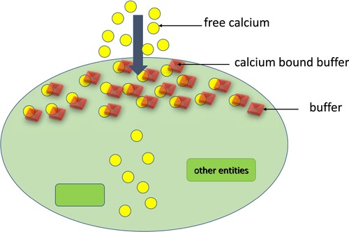
Diagrammatically showed in Figure 1, the main element of the $\text{C}{a}^{+2}$ buffering in central neurons. Free $\text{C}{a}^{+2}$ ions enter the cytoplasm through the voltage-gated $\text{C}{a}^{+2}$ channels (VGCC). And buffers bind to calcium ions to form a calcium-bound buffer.

Figure 1. Diagrammatic representation of calcium buffering.

The following is the bidirectional reaction between $\text{C}{a}^{+2}$ and buffer: $\mathtt{C}+\mathtt{B}\underset{L_j^{-}}{\stackrel{L_j^{+}}{\rightleftharpoons }}\mathtt{C}\mathtt{B},$here $\mathtt{B}$ denotes the free buffer, $\mathtt{C}$ the free $\text{C}{a}^{+2}$ ion, and $\mathtt{C}\mathtt{B}$ the buffer that is calcium-bound.

The following equations for changes in Ca concentration, free buffer, and calcium bound buffers are generated based on the assumption that the calcium-buffer association process follows mass action kinetics. (4) $\begin{array}{rl}& \frac{\mathrm{\partial }\left[\mathtt{C}\right]}{\mathrm{\partial }t}=\Omega {\mathrm{\nabla }}^2\left[\mathtt{C}\right]+\sum _j{\zeta }_j,\\ & \frac{\mathrm{\partial }\left[\mathtt{B}\right]}{\mathrm{\partial }t}=\gamma {\mathrm{\nabla }}^2\left[\mathtt{B}\right]+\sum _j{\zeta }_j,\\ & \frac{\mathrm{\partial }\left[\mathtt{C}\mathtt{B}\right]}{\mathrm{\partial }t}=\omega {\mathrm{\nabla }}^2\left[\mathtt{C}\mathtt{B}\right]-\sum _j{\zeta }_j,\end{array}\}$(4) here Ω denotes the diffusion coefficient for free $\text{C}{a}^{+2}$ ion, γ the free buffer, and ω the buffer that is calcium bound. For the buffer concentration, ${\zeta }_j$ represents the reaction term, which becomes represented including a conjunction with the association rate constant and the dissociation rate constant: (5) ${\zeta }_j=-L_j^{+}\left[\mathtt{B}\right]\left[\mathtt{C}\right]+L_j^{-}\left[\mathtt{C}\mathtt{B}\right],$(5) and $L_1$ and $L_2$ represent the association and dissociation rate constants, respectively, while buffer j.

Assuming $\left[\mathtt{C}\right]=\mathcal{X},\left[\mathtt{B}\right]=\mathcal{Y}$ thus $\left[\mathtt{C}\mathtt{B}\right]=\mathcal{Z}$. Setting $\gamma =\omega =0$ is used to account for those buffers that do not disperse and are categorized as permanent and immovable. The model's mathematical form is (6) $\frac{\mathrm{\partial }\mathcal{X}}{\mathrm{\partial }t}=\Omega \frac{{\mathrm{\partial }}^2\mathcal{X}}{\mathrm{\partial }{x}^2}-v\frac{\mathrm{\partial }\mathcal{X}}{\mathrm{\partial }x}-L_j\mathcal{Y}(\mathcal{X}-{\mathcal{X}}_{\mathrm{\infty }}).$(6) The conditions are as follows: (7) $\begin{array}{rl}& \mathcal{X}(x,0)=f\left(x\right),t=0,x>0,\\ & \mathcal{X}(0,t)={\mathcal{X}}_0,t>0,x\ge 0,\\ & \frac{\mathrm{\partial }\mathcal{X}}{\mathrm{\partial }x}=0,t\ge 0,x\to \mathrm{\infty }.\end{array}\}$(7) Now, replacing $W$ with $\mathcal{X}-{\mathcal{X}}_{\mathrm{\infty }}$ and also assuming $L_j\mathcal{Y}=g$, the above system reduces to: (8) $\frac{\mathrm{\partial }W}{\mathrm{\partial }t}=\Omega \frac{{\mathrm{\partial }}^{2}W}{\mathrm{\partial }{x}^2}-v\frac{\mathrm{\partial }W}{\mathrm{\partial }x}-gW,$(8) with conditions: (9) $\begin{array}{rl}& W(x,0)=f\left(x\right)-{\mathcal{X}}_{\mathrm{\infty }},t=0,x>0,\\ & W(0,t)={\mathcal{X}}_0-{\mathcal{X}}_{\mathrm{\infty }},t>0,x\ge 0,\\ & \frac{\mathrm{\partial }W}{\mathrm{\partial }x}=0,t\ge 0,x\to \mathrm{\infty }.\end{array}\}$(9) On utilizing non-dimensionalization variables $x^{\ast }=x\sqrt{\frac{g}{\Omega }},t^{\ast }=gt,W^{\ast }=\frac{W}{{\mathcal{X}}_0},q=\frac{v}{\sqrt{g\Omega }}$ in the set of Equation (8(8) $\frac{\mathrm{\partial }W}{\mathrm{\partial }t}=\Omega \frac{{\mathrm{\partial }}^{2}W}{\mathrm{\partial }{x}^2}-v\frac{\mathrm{\partial }W}{\mathrm{\partial }x}-gW,$(8) ) we get (10) $\frac{\mathrm{\partial }W}{\mathrm{\partial }t}=\frac{{\mathrm{\partial }}^{2}W}{\mathrm{\partial }{x}^2}-q\frac{\mathrm{\partial }W}{\mathrm{\partial }x}-W,$(10) conditions: (11) $\begin{array}{rl}& W(x,0)=\frac{f\left(x\right)-{\mathcal{X}}_{\mathrm{\infty }}}{{\mathcal{X}}_0},t=0,x>0,\\ & W(0,t)=\frac{{\mathcal{X}}_0-{\mathcal{X}}_{\mathrm{\infty }}}{{\mathcal{X}}_0},t>0,x\ge 0,\\ & \frac{\mathrm{\partial }W}{\mathrm{\partial }x}=0,t\ge 0,x\to \mathrm{\infty }.\end{array}\}$(11) When $W(x,t)={\mathrm{e}}^{\frac{qx}{2}}\varphi (x,t)$ [33] is implemented, then Equation (10(10) $\frac{\mathrm{\partial }W}{\mathrm{\partial }t}=\frac{{\mathrm{\partial }}^{2}W}{\mathrm{\partial }{x}^2}-q\frac{\mathrm{\partial }W}{\mathrm{\partial }x}-W,$(10) ) is simplified to the following form: (12) $\frac{\mathrm{\partial }\varphi }{\mathrm{\partial }t}=\frac{{\mathrm{\partial }}^2\varphi }{\mathrm{\partial }{x}^2}-(\frac{q^2}{2}+1)\varphi .$(12) Now, substituting ${\vartheta }^2=\frac{q^2}{2}+1$ in Equation (12(12) $\frac{\mathrm{\partial }\varphi }{\mathrm{\partial }t}=\frac{{\mathrm{\partial }}^2\varphi }{\mathrm{\partial }{x}^2}-(\frac{q^2}{2}+1)\varphi .$(12) ) then obtains: (13) $\frac{\mathrm{\partial }\varphi }{\mathrm{\partial }t}=\frac{{\mathrm{\partial }}^2\varphi }{\mathrm{\partial }{x}^2}-{\vartheta }^2\varphi ,$(13) corresponding conditions: (14) $\begin{array}{rl}& \varphi (x,0)=\frac{f\left(x\right)-{\mathcal{X}}_{\mathrm{\infty }}}{{\mathcal{X}}_0},t=0,x>0,\\ & \varphi (0,t)=\frac{{\mathcal{X}}_0-{\mathcal{X}}_{\mathrm{\infty }}}{{\mathcal{X}}_0},t>0,x\ge 0,\\ & li{m}_{x\to \mathrm{\infty }}\varphi (x,t)=0.\end{array}\}$(14) Now, using the Hilfer fractional derivative, fractionalize (13(13) $\frac{\mathrm{\partial }\varphi }{\mathrm{\partial }t}=\frac{{\mathrm{\partial }}^2\varphi }{\mathrm{\partial }{x}^2}-{\vartheta }^2\varphi ,$(13) ) w.r.t time variable, (15) ${\mathcal{D}}_t^{\mu ,\sigma }\varphi (x,t)=\frac{{\mathrm{\partial }}^2\varphi }{\mathrm{\partial }{x}^2}-{\vartheta }^2\varphi ,$(15) with conditions: (16) $\begin{array}{rl}& \varphi (x,0)=\frac{f\left(x\right)-{\mathcal{X}}_{\mathrm{\infty }}}{{\mathcal{X}}_0},t=0,x>0,\\ & \varphi (0,t)=\frac{{\mathcal{X}}_0-{\mathcal{X}}_{\mathrm{\infty }}}{{\mathcal{X}}_0},t>0,x\ge 0,\\ & li{m}_{x\to \mathrm{\infty }}\varphi (x,t)=0.\end{array}\}$(16) Applying the LT on Equation (15(15) ${\mathcal{D}}_t^{\mu ,\sigma }\varphi (x,t)=\frac{{\mathrm{\partial }}^2\varphi }{\mathrm{\partial }{x}^2}-{\vartheta }^2\varphi ,$(15) ) concerning the time variable, we obtain: ${\mathcal{S}}^{\sigma }\overline{\varphi }(x,\mathcal{S})-{\mathcal{S}}^{\mu (\sigma -1)}{\mathcal{I}}^{(1-\mu )(1-\sigma )}\varphi (x,0)=\frac{{\mathrm{\partial }}^2\overline{\varphi }(x,\mathcal{S})}{\mathrm{\partial }{x}^2}-{\vartheta }^2\overline{\varphi }(x,\mathcal{S}),$taking ${\mathcal{I}}^{(1-\mu )(1-\sigma )}\varphi (x,0)=\mathcal{F}\left(x\right)$, (17) ${\mathcal{S}}^{\sigma }\overline{\varphi }(x,\mathcal{S})-{\mathcal{S}}^{\mu (\sigma -1)}\mathcal{F}\left(x\right)=\frac{{\mathrm{\partial }}^2\overline{\varphi }(x,\mathcal{S})}{\mathrm{\partial }{x}^2}-{\vartheta }^2\overline{\varphi }(x,\mathcal{S}).$(17) The LT of $\varphi (x,t)$ w.r.t time variable t is represented by $\overline{\varphi }(x,\mathcal{S})$. Now we apply the FT to the space variable using Equation (17(17) ${\mathcal{S}}^{\sigma }\overline{\varphi }(x,\mathcal{S})-{\mathcal{S}}^{\mu (\sigma -1)}\mathcal{F}\left(x\right)=\frac{{\mathrm{\partial }}^2\overline{\varphi }(x,\mathcal{S})}{\mathrm{\partial }{x}^2}-{\vartheta }^2\overline{\varphi }(x,\mathcal{S}).$(17) ), and we get: (18) $\begin{array}{rl}& {\mathcal{S}}^{\sigma }\hat{\overline{\varphi }}(\mathcal{P},\mathcal{S})-{\mathcal{S}}^{\mu (\sigma -1)}\hat{\mathcal{F}}\left(\mathcal{P}\right)=-{\mathcal{P}}^2\hat{\overline{\varphi }}(\mathcal{P},\mathcal{S})-{\vartheta }^2\hat{\overline{\varphi }}(\mathcal{P},\mathcal{S}),\end{array}$(18) (19) $\begin{array}{rl}& \hat{\overline{\varphi }}(\mathcal{P},\mathcal{S})=\frac{{\mathcal{S}}^{\mu (\sigma -1)}\hat{\mathcal{F}}\left(\mathcal{P}\right)}{{\mathcal{S}}^{\sigma }+{\vartheta }^2+{\mathcal{P}}^2},\end{array}$(19) the FT of $\varphi (x,\mathcal{S})$ w.r.t space variable x is represented by $\hat{\overline{\varphi }}(\mathcal{P},\mathcal{S})$.

Applying the inverse LT to Equation (19(19) $\begin{array}{rl}& \hat{\overline{\varphi }}(\mathcal{P},\mathcal{S})=\frac{{\mathcal{S}}^{\mu (\sigma -1)}\hat{\mathcal{F}}\left(\mathcal{P}\right)}{{\mathcal{S}}^{\sigma }+{\vartheta }^2+{\mathcal{P}}^2},\end{array}$(19) ) obtains: (20) $\hat{\varphi }(\mathcal{P},t)=t^{\sigma -\sigma \mu +\mu -1}{E}_{\sigma ,\sigma -\sigma \mu +\mu }(-({\mathcal{P}}^2+{\vartheta }^2\left)t^{\sigma }\right)\hat{\mathcal{F}}\left(\mathcal{P}\right).$(20) Now, applying the inverse FT to Equation (20(20) $\hat{\varphi }(\mathcal{P},t)=t^{\sigma -\sigma \mu +\mu -1}{E}_{\sigma ,\sigma -\sigma \mu +\mu }(-({\mathcal{P}}^2+{\vartheta }^2\left)t^{\sigma }\right)\hat{\mathcal{F}}\left(\mathcal{P}\right).$(20) ) yields, (21) $\begin{array}{rl}\varphi (x,t)& =\frac{1}{2\pi }{\int }_{-\mathrm{\infty }}^{\mathrm{\infty }}{t}^{\sigma -\sigma \mu +\mu -1}{\mathrm{e}}^{-\iota \mathcal{P}x}{E}_{\sigma ,\sigma -\sigma \mu +\mu }(-({\mathcal{P}}^2+{\vartheta }^2\left)t^{\sigma }\right)\hat{\mathcal{F}}\left(\mathcal{P}\right)\mathrm{d}\mathcal{P},\\ \varphi (x,t)& =\frac{t^{\sigma -\sigma \mu +\mu -1}}{2\pi }{\int }_{-\mathrm{\infty }}^{\mathrm{\infty }}{\mathrm{e}}^{-\iota \mathcal{P}x}{E}_{\sigma ,\sigma -\sigma \mu +\mu }(-({\mathcal{P}}^2+{\vartheta }^2\left)t^{\sigma }\right)\left({\int }_{-\mathrm{\infty }}^{\mathrm{\infty }}{\mathrm{e}}^{\iota \mathcal{P}y}\mathcal{F}\right(y\left)\mathrm{d}y\right)\mathrm{d}\mathcal{P}.\end{array}$(21) As a result, by applying $W(x,t)={\mathrm{e}}^{\frac{qx}{2}}\varphi (x,t)$, we arrive at the following conclusions: (22) $\begin{array}{rl}W(x,t)& =\frac{t^{\sigma -\sigma \mu +\mu -1}}{2\pi }{\mathrm{e}}^{\frac{qx}{2}}{\int }_{-\mathrm{\infty }}^{\mathrm{\infty }}{\mathrm{e}}^{-\iota \mathcal{P}x}{E}_{\sigma ,\sigma -\sigma \mu +\mu }(-({\mathcal{P}}^2+{\vartheta }^2\left)t^{\sigma }\right)\\ & \times \left({\int }_{-\mathrm{\infty }}^{\mathrm{\infty }}{\mathrm{e}}^{\iota \mathcal{P}y}\mathcal{F}\right(y\left)\mathrm{d}y\right)\mathrm{d}\mathcal{P},\\ & ={\mathrm{e}}^{\frac{qx}{2}}{\int }_{-\mathrm{\infty }}^{\mathrm{\infty }}\left(\frac{t^{\sigma -\sigma \mu +\mu -1}}{2\pi }{\int }_{-\mathrm{\infty }}^{\mathrm{\infty }}{\mathrm{e}}^{-\iota \mathcal{P}(x-y)}{E}_{\sigma ,\sigma -\sigma \mu +\mu }(-({\mathcal{P}}^2+{\vartheta }^2\left)t^{\sigma }\right)\mathrm{d}\mathcal{P}\right)\\ & \times \mathcal{F}\left(y\right)\mathrm{d}y,\\ & ={\mathrm{e}}^{\frac{qx}{2}}{\int }_{-\mathrm{\infty }}^{\mathrm{\infty }}G(x-y,t)\mathcal{F}\left(y\right)\mathrm{d}y,\end{array}$(22) here (23) $G(x,t)=\frac{t^{\sigma -\sigma \mu +\mu -1}}{2\pi }{\int }_{-\mathrm{\infty }}^{\mathrm{\infty }}{\mathrm{e}}^{-\iota \mathcal{P}x}{E}_{\sigma ,\sigma -\sigma \mu +\mu }(-({\mathcal{P}}^2+{\vartheta }^2\left)t^{\sigma }\right)\mathrm{d}\mathcal{P}.$(23)

4. Special cases and application

In this section, we study exceptional cases and applications. Taking some particular values of fractional order derivatives in Hilfer derivatives, we get Caputo and RL derivatives. Here, if we put $\mu =1$ and $\mu =0$ in the Hilfer derivative, we get Caputo and RL fractional derivatives, respectively.

Theorem 4.1

Consider the following fractionalized Equation (15(15) ${\mathcal{D}}_t^{\mu ,\sigma }\varphi (x,t)=\frac{{\mathrm{\partial }}^2\varphi }{\mathrm{\partial }{x}^2}-{\vartheta }^2\varphi ,$(15) ) with respect to time, (24) ${}^C{\mathcal{D}}_t^{\sigma }\varphi (x,t)=\frac{{\mathrm{\partial }}^2\varphi }{\mathrm{\partial }{x}^2}-{\vartheta }^2\varphi ,$(24) where ${}^C{\mathcal{D}}_t^{\sigma }$ is the fractional derivative in Caputo sense. The corresponding conditions are, $\begin{array}{rl}& \varphi (x,0)=\frac{f\left(x\right)-{\mathcal{X}}_{\mathrm{\infty }}}{{\mathcal{X}}_0},t=0,x>0,\\ & \varphi (0,t)=\frac{{\mathcal{X}}_0-{\mathcal{X}}_{\mathrm{\infty }}}{{\mathcal{X}}_0},t>0,x\ge 0,\\ & li{m}_{x\to \mathrm{\infty }}\varphi (x,t)=0,\end{array}$and $W(x,t)={\mathrm{e}}^{\frac{qx}{2}}\varphi (x,t)$.

With the given condition, the solution to the above equation is (25) $W(x,t)={\mathrm{e}}^{\frac{qx}{2}}{\int }_{-\mathrm{\infty }}^{\mathrm{\infty }}G(x-y,t)\mathcal{F}\left(y\right)\mathrm{d}y,$(25) here (26) $G(x,t)=\frac{1}{2\pi }{\int }_{-\mathrm{\infty }}^{\mathrm{\infty }}{\mathrm{e}}^{-\iota \mathcal{P}x}{E}_{\sigma ,1}(-({\mathcal{P}}^2+{\vartheta }^2\left)t^{\sigma }\right)\mathrm{d}\mathcal{P}.$(26)

Theorem 4.2

Consider the following fractionalized Equation (15(15) ${\mathcal{D}}_t^{\mu ,\sigma }\varphi (x,t)=\frac{{\mathrm{\partial }}^2\varphi }{\mathrm{\partial }{x}^2}-{\vartheta }^2\varphi ,$(15) ) with respect to time, (27) ${}^{RL}{\mathcal{D}}_t^{\sigma }\varphi (x,t)=\frac{{\mathrm{\partial }}^2\varphi }{\mathrm{\partial }{x}^2}-{\vartheta }^2\varphi ,$(27) where ${}^{RL}{\mathcal{D}}_t^{\sigma }$ is the fractional derivative in RL sense. The corresponding conditions are, $\begin{array}{rl}& \varphi (x,0)=\frac{f\left(x\right)-{\mathcal{X}}_{\mathrm{\infty }}}{{\mathcal{X}}_0},t=0,x>0,\\ & \varphi (0,t)=\frac{{\mathcal{X}}_0-{\mathcal{X}}_{\mathrm{\infty }}}{{\mathcal{X}}_0},t>0,x\ge 0,\\ & li{m}_{x\to \mathrm{\infty }}\varphi (x,t)=0,\end{array}$and $W(x,t)={\mathrm{e}}^{\frac{qx}{2}}\varphi (x,t)$.

With the given condition, the solution to the above equation is (28) $W(x,t)={\mathrm{e}}^{\frac{qx}{2}}{\int }_{-\mathrm{\infty }}^{\mathrm{\infty }}G(x-y,t)\mathcal{F}\left(y\right)\mathrm{d}y,$(28) here (29) $G(x,t)=\frac{t^{\sigma -1}}{2\pi }{\int }_{-\mathrm{\infty }}^{\mathrm{\infty }}{\mathrm{e}}^{-\iota \mathcal{P}x}{E}_{\sigma ,\sigma }(-({\mathcal{P}}^2+{\vartheta }^2\left)t^{\sigma }\right)\mathrm{d}\mathcal{P}.$(29)

Application: Here we discuss the certain applications of our main theorem in Section 3 for the function $f\left(x\right)=\delta \left(x\right)$.

Corollary 4.3

Consider the following fractionalised equation w.r.t time, (30) $\begin{array}{rl}& {\mathcal{D}}_t^{\mu ,\sigma }\varphi (x,t)=\frac{{\mathrm{\partial }}^2\varphi }{\mathrm{\partial }{x}^2}-{\vartheta }^2\varphi ,\\ with\\ & {\mathcal{I}}^{(1-\mu )(1-\sigma )}\varphi (x,0)=0,0<\mu \le 1,0\le \sigma \le 1,\\ & \varphi (0,t)=\frac{{\mathcal{X}}_0-{\mathcal{X}}_{\mathrm{\infty }}}{{\mathcal{X}}_0},t>0,x\ge 0,\\ & li{m}_{x\to \mathrm{\infty }}\varphi (x,t)=0.\end{array}$(30) $The concentration $W(x,t)$ is (31) $W(x,t)={\mathrm{e}}^{\frac{qx}{2}}{\int }_{-\mathrm{\infty }}^{\mathrm{\infty }}G(x-y,t)\delta \left(y\right)\mathrm{d}y,$(31) here (32) $G(x,t)=\frac{t^{\sigma -\sigma \mu +\mu -1}}{2\pi }{\int }_{-\mathrm{\infty }}^{\mathrm{\infty }}{\mathrm{e}}^{-\iota \mathcal{P}x}{E}_{\sigma ,\sigma -\sigma \mu +\mu }(-({\mathcal{P}}^2+{\vartheta }^2\left)t^{\sigma }\right)\mathrm{d}\mathcal{P}.$(32)

5. Illustration and discussion

This segment shows the Ca profile against various biophysical parameters via Matlab, which shows in Table 1. Figure 2 shows that the calcium profile is different over time for the RL case, which corresponds to $\mu =0$, and plots are taken for $\sigma =1,0.9,0.8$. The cytosolic concentration level drops below the 0.5 μM level and reaches a steady state close to 0.3 μM. As the fractional derivative order drops, the whole flow behaviour stays at substantially reduced levels, and the concentration declines separately. This is due to the ions diffusing out and interacting with the buffers.

Figure 2. Graph among of $W(x,t)$ and t for various σ values for $\mu =0$ which corresponds to the RL derivative. (a) EGTA, (b) Troponine, (c) Calmodulin, and (d) BAPTA.

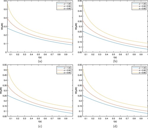
Table 1. List of physiological parameters [34].

Symbol	Parameter	Values
Ω	Diffusion coefficient	200–300 $\mu {\mathrm{m}}^2{\mathrm{s}}^{-1}$
v	Velocity	10–100 $\mu {\mathrm{m}\mathrm{s}}^{-1}$
${\mathcal{X}}_{\mathrm{\infty }}$	Background calcium concentration	0.1 μM
$\mathcal{Y}$	Buffer concentration	2–350 μM
$L_1$ EGTA	Buffer association rate	1.5 $\mu {\mathrm{M}}^{-1}{s}^{-1}$
$L_1$ Troponine	Buffer association rate	90 $\mu {\mathrm{M}}^{-1}{s}^{-1}$
$L_1$ Calmodulin	Buffer association rate	250 $\mu {\mathrm{M}}^{-1}{s}^{-1}$
$L_1$ BAPTA	Buffer association rate	600 $\mu {\mathrm{M}}^{-1}{s}^{-1}$

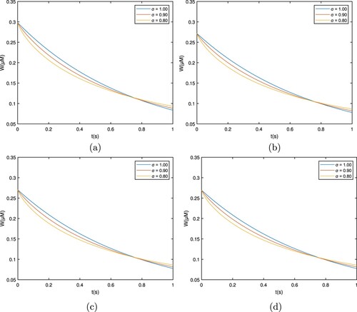
Figure 3 shows that the calcium profile is different over time for the Caputo case, which corresponds to $\mu =1$, and plots are taken for $\sigma =1,0.9,0.8$. The cytosolic concentration level drops below the 0.15 μM level and reaches a steady state close to 0.3 μM. As the fractional derivative order drops, the whole flow profile stays at lower levels, and the concentration declines separately. This is due to the ions diffusing out and interacting with the buffers.

Figure 3. Graph among of $W(x,t)$ and t for various σ values for $\mu =0$ which corresponds to the Caputo derivative. (a) EGTA, (b) Troponine, (c) Calmodulin, and (d) BAPTA.

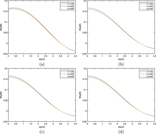
Figures 4 and 5 show the space-related variation in the RL case and Caputo derivative, which corresponds to $\mu =0$, and $\mu =1$ respectively. Figures 4 and 5 show the interpretation of the Ca concentration profile including a location by various qualities through the fractional order $\sigma =1,0.9,0.8$. The concentration of free $\text{C}{a}^{+2}$ ions is seen to be high at the entrance site; when calcium ions spread and bind to the buffer, the concentration of free $\text{C}{a}^{+2}$ ions diminishes.

Figure 4. Graph among of $W(x,t)$ and x for various σ values for $\mu =0$ which corresponds to the RL derivative. (a) EGTA, (b) Troponine, (c) Calmodulin, and (d) BAPTA.

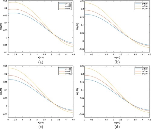
Figure 5. Graph among of $W(x,t)$ and x for various σ values for $\mu =0$ which corresponds to the Caputo derivative. (a) EGTA, (b) Troponine, (c) Calmodulin, and (d) BAPTA.

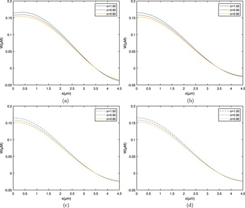
As it interacts with the buffer, the greatest amount near the entrance site lowers the cytosolic calcium concentration. The whole pattern shifts to the upper side as the fractional order rises.

The curves in Figures 4, 5, and 7 demonstrate that the overall flow profile diminishes and enters a steady state when the order σ of the fractional derivative decreases. Additionally, it drops sharply for the integral value of σ.

Figure 6. Graph among of $W(x,t)$ and t for various σ values for $\mu =0.9$. (a) EGTA, (b) Troponine, (c) Calmodulin, and (d) BAPTA.

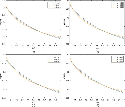
Figure 7. Graph among of $W(x,t)$ and x for various σ values for $\mu =0.9$. (a) EGTA, (b) Troponine, (c) Calmodulin, and (d) BAPTA.

The increase in concentration levels after reaching the cytosol and right before interacting with the buffer is due to a non-local characteristic of the fractional operator. Cytosolic calcium concentration level in Figure 6 at the starting level, $\text{C}{a}^{+2}$ ions react with the buffer species and, therefore, the Ca concentration decreases significantly. After this, a steady state is obtained.

Figures 8 and 10 show the temporal distribution for the endogenous buffers EGTA and BAPTA. On the starting position, the concentration level for both buffers is extremely high and gradually decreases; It reflects that kind of change in the amount of free $\text{C}{a}^{+2}$ ion concentration. Near the entry point, their concentration approaches 0.4 μM and decreases as $\text{C}{a}^{+2}$ ions begin associating with the buffer, reaching the lowest level of 0.4 μM.

Figure 8. Graph for the buffers EGTA and BAPTA with $\sigma =0.9$ between $W(x,t)$ and t. (a) $\mu =0$, (b) $\mu =0.8$, (c) $\mu =0.9$, and (d) $\mu =1$.

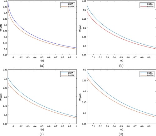
It is also observed that the overall pattern for EGTA is (little) higher than that for BAPTA, indicating so it EGTA is a slower buffer than BAPTA.

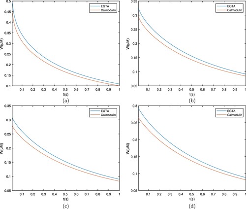
Figures 9 and 11 depict spatial Ca concentration patterns for exogenous buffers EGTA along with calmodulin. The intracellular Ca content grows, whereas calmodulin falls as it spreads and attaches to the buffer, even so the overall pattern regarding EGTA buffer stays high.

Figure 9. Graph between $W(x,t)$ and t for buffers EGTA and Calmodulin with $\sigma =0.9$. (a) $\mu =0$, (b) $\mu =0.8$, (c) $\mu =0.9$, and (d) $\mu =1$.

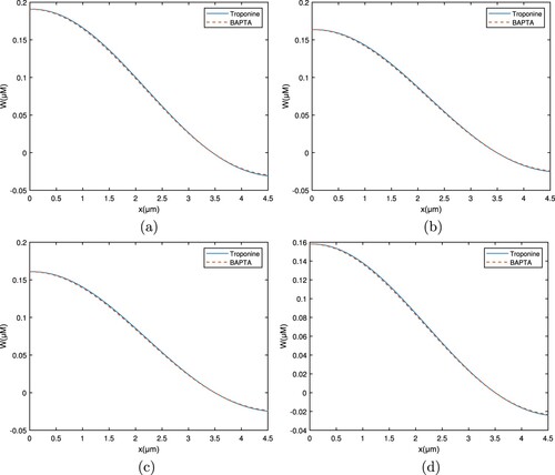
Similarly, Figures 12 and 13 demonstrate the calcium distribution for troponine and BAPTA, respectively. It is obvious from the troponine curve that the Ca concentration level increases quickly and then declines fast. Nonetheless, the overall calcium concentration profile remained greater than BAPTA. The variation in calcium concentrations about different buffers results from their affinity for other Ca. With a low $\text{C}{a}^{+2}$ affinity buffer, there are less binding of $\text{C}{a}^{+2}$ ions in the cytosol and a higher concentration of free $\text{C}{a}^{+2}$ ions.

When the whole intracellular calcium concentration profile is compared, it is discovered that the concentration of free $\text{C}{a}^{+2}$ ions for EGTA is more than for BAPTA. This distinction is because EGTA moves slowly while BAPTA is a quick chelator. BAPTA aids between the reduction of cellular Ca and protects cells against calcium toxicity.

Figure 10. Graph for the buffers EGTA and BAPTA with $\sigma =0.9$ between $W(x,t)$ and x. (a) $\mu =0$, (b) $\mu =0.8$, (c) $\mu =0.9$, and (d) $\mu =1$.

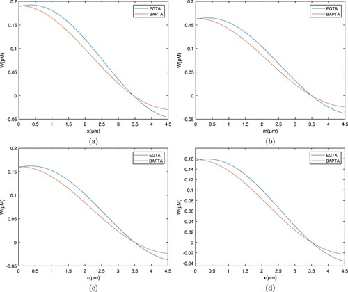
Figure 11. Graph for the buffers EGTA and Calmodulin with $\sigma =0.9$ between $W(x,t)$ and x. (a) $\mu =0$, (b) $\mu =0.8$, (c) $\mu =0.9$, and (d) $\mu =1$.

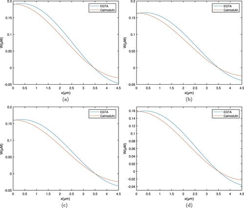
Figure 12. Graph for the buffers Troponine and BAPTA with $\sigma =0.9$ between $W(x,t)$ and t. (a) $\mu =0$, (b) $\mu =0.8$, (c) $\mu =0.9$, and (d) $\mu =1$.

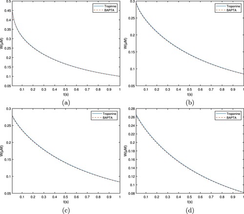
Figure 13. Graph for the buffers Troponine and BAPTA with $\sigma =0.9$ between $W(x,t)$ and x. (a) $\mu =0$, (b) $\mu =0.8$, (c) $\mu =0.9$, and (d) $\mu =1$.

6. Conclusions

This paper presents the physiological phenomenon of the distribution of cytosolic calcium concentration using a Hilfer derivative. The model uses advection diffusion with calcium-binding buffers. Concentration effects are discussed for EGTA, Troponine, Calmodulin, and BAPTA. Calcium buffers affect signalling. The fractional order derivative is more favourable than the integer order since the future state of the system relies on its present state and all its previous circumstances. The model solution is found using integral transform and removing RL and Caputo derivatives. Simulations indicate fractional ordering's influence on calcium profile. Combined, for every buffer taking into account in this work, is therefore noticed that calcium concentration begins to decrease after entering the cell as $\text{C}{a}^{+2}$ ions initiate to react among the buffer species. Different buffers reduce concentration in a different manners. EGTA's concentration profile is greater than BAPTA's. EGTA is a slow buffer, whereas BAPTA is a quick chelator. The fractional operator's non-locality is reflected in this same increase in concentration and upon attempting to enter the cytosol and before interacting along the buffer. Clearly, buffers affect the calcium profile. The buffer decreases cellular calcium and avoids toxicity. Calcium-binding buffer impacts temporal and spatial calcium transients.

Calcium profile is of great importance in the biological sciences. In this paper, we describe the processing of calcium buffer bonding in humans with the help of a calcium buffer bonding model, which is essential from a mathematical and computational point of view. Calcium buffer bonding will be more precisely understood if the paper's numerical results are used in a medical environment. Parameters such as a person's blood volume, blood pressure, weight, body temperature, abdominal size, age, etc., can be included in the simulation to increase its accuracy. By analysing the critical facts discussed in all sections and concluding remarks, the clinician or researcher may use the results of this article to evaluate calcium buffer binding.

These models can be improved to produce spatiotemporal patterns of calcium-buffered concentration in reaction to a particular activity through precise synchronization of transport mechanisms. The information generated by these models can be beneficial for biomedical researchers to comprehend the accurate physical coordination of cellular processes and the disruptions of this coordination, which can lead to the creation of protocols for detecting and treating neuronal diseases. Its accuracy for the general populace can also be tested with additional studies. The connection between biophysical factors, such as pump, leak, diffusion, coefficient, and others, can be further explored using efficient models. They can also be used to examine the effects of fractional convective diffusion on the spread of calcium buffer in the presence of an intrinsic process.

Authors' contributions

SB and KJ a made significant contributions to the creation of the work. SS and SDP contributed to the design of the work and handled the analysis. DB conceptualized and doublechecked the Analysis part. DLS was involved in the manuscript's drafting or critical revision for important intellectual content. All authors read and approved the final version of manuscript.

Acknowledgments

The authors express their sincere thanks to the editor and reviewers for their fruitful comments and suggestions that improved the quality of the manuscript.

Disclosure statement

No potential conflict of interest was reported by the author(s).

Funding

No funding was received for conducting this study.

Availability of data and materials

No data sets were generated or analysed during the current study.

References

- Jafri MS, Keizer J. On the roles of Ca2+ diffusion, Ca2+ buffers, and the endoplasmic reticulum in IP3-induced Ca2+ waves. Biophys J. 1995;69(5):2139–2153.
- Habenom H, Aychluh M, Suthar DL, et al. Modeling and analysis on the transmission of covid-19 pandemic in Ethiopia. Alex Eng J. 2022;61(7):5323–5342.
- Wang Y, Liu S, Khan A. On fractional coupled logistic maps: chaos analysis and fractal control. Nonlinear Dyn. 2023;111(6):5889–5904.
- Shyamsunder, Bhatter S, Jangid K, Abidemi A, et al. A new fractional mathematical model to study the impact of vaccination on COVID-19 outbreaks. Decis Anal J. 2023;6:100156.
- Meyer T, Stryer L. Molecular model for receptor-stimulated calcium spiking. Proc Natl Acad Sci India. 1988;85(14):5051–5055.
- Neher E. Concentration profiles of intracellular calcium in the presence of a diffusible chelator. Exp Brain Res. 1986;14:80–96.
- Winston F, Thibault L, Macarak E. An analysis of the time-dependent changes in intracellular calcium concentration in endothelial cells in culture induced by mechanical stimulation. J Biomech Eng. 1993;115(2):160–168.
- Smith GD, Wagner J, Keizer J. Validity of the rapid buffering approximation near a point source of calcium ions. Biophys J. 1996;70(6):2527–2539.
- Agarwal R, Kritika N, Purohit SD, et al. Mathematical modelling of cytosolic calcium concentration distribution using non-local fractional operator. Discrete Contin Dyn Syst, Ser S. 2021;14(10):3387–3399.
- Jha BK, Adlakha N, Mehta MN. Finite volume model to study the effect of buffer on cytosolic Ca2+ advection diffusion. Int J Eng Nat Sci. 2010;4(3):160–163.
- Tripathi A, Adlakha N. Finite volume model to study calcium diffusion in neuron cell under excess buffer approximation. Int J Math Sci Engg Appls. 2011;5:437–447.
- Agarwal R, Kritika N, Purohit SD. Mathematical model pertaining to the effect of buffer over cytosolic calcium concentration distribution. Chaos Solit Fractals. 2021;143:110610.
- Eskandari Z, Avazzadeh Z, Khoshsiar Ghaziani R, et al. Dynamics and bifurcations of a discrete-time Lotka–Volterra model using nonstandard finite difference discretization method. Math Methods Appl Sci. 2022: 1–16. doi:10.1002/mma.8859.
- Li B, Liang H, He Q. Multiple and generic bifurcation analysis of a discrete Hindmarsh-Rose model. Chaos Solit Fractals. 2021;146:110856.
- Kumawat S, Bhatter S, Suthar DL, et al. Numerical modeling on age-based study of coronavirus transmission. Appl Math Sci Eng (AMSE). 2022;30(1):609–634.
- Khan A, Alshehri HM, Gómez-Aguilar J, et al. A predator–prey model involving variable-order fractional differential equations with Mittag-Leffler kernel. Adv Differ Equ. 2021;183:1–18.
- Kumar V, Malik M, Baleanu D. Results on Hilfer fractional switched dynamical system with non-instantaneous impulses. Pramana. 2022;96(1):1–15.
- Khan A, Alshehri HM, Abdeljawad T, et al. Stability analysis of fractional nabla difference COVID-19 model. Results Phys. 2021;22:103888.
- El-Sayed A, Baleanu D, Agarwal P. A novel jacobi operational matrix for numerical solution of multi-term variable-order fractional differential equations. J Taibah Univ Sci. 2020;14(1):963–974.
- Devi A, Kumar A, Baleanu D, et al. On stability analysis and existence of positive solutions for a general non-linear fractional differential equations. Adv Differ Equ. 2020;300:1–16.
- Etemad S, Avci I, Kumar P, et al. Some novel mathematical analysis on the fractal–fractional model of the AH1N1/09 virus and its generalized caputo-type version. Chaos Solit Fractals. 2022;162:112511.
- Aychluh M, Purohit SD, Agarwal P, et al. Atangana–Baleanu derivative-based fractional model of COVID-19 dynamics in Ethiopia. Appl Math Sci Eng (AMSE). 2022;30(1):634–659.
- Baleanu D, Agarwal RP, Parmar RK, et al. Extension of the fractional derivative operator of the Riemann-Liouville. J Nonlinear Sci Appl. 2017;10:2914–2924.
- Shyamsunder, Bhatter S, Jangid K, Purohit SD. Fractionalized mathematical models for drug diffusion. Chaos Solit Fractals. 2022;165:112810.
- Khan H, Gomez-Aguilar J, Abdeljawad T, et al. Existence results and stability criteria for ABC-fuzzy-Volterra integro-differential equation. Fractals. 2020;28(08):2040048.
- Hilfer R. Applications of fractional calculus in physics. Singapore: World scientific; 2000.
- Mittag-Leffler SM. On the new function Eα(x). CR Acad Sci Paris. 1903;137(2):554–558.
- Wiman A. Üabout the fundamental theorem in the theory of functions Ea(x). Acta Math. 1905;29:191–201.
- Sneddon IN. Fourier transforms. New York: McGraw-Hill Book Co., Inc; 1951.
- Shyamsunder, Bhatter S, Jangid K, Purohit SD. A study of the hepatitis B virus infection using hilfer fractional derivative. PIMM. 2022;48:100–117.
- Miller KS, Ross B. An introduction to the fractional calculus and fractional differential equations. New Jersey, USA: Wiley; 1993.
- Tomovski Ž. Generalized Cauchy type problems for nonlinear fractional differential equations with composite fractional derivative operator. Nonlinear Anal, Theory Methods Appl. 2012;75(7):3364–3384.
- Rubbab Q, Mirza IA, Qureshi MZA. Analytical solutions to the fractional advection-diffusion equation with time-dependent pulses on the boundary. AIP Adv. 2016;6(7):075318.
- Tripathi A, Adlakha N. Finite volume model to study calcium diffusion in neuron cell under excess buffer approximation. Int J Math Sci Eng Appl. 2011;5:437–447.