Dynamic response analysis of fractional order RLC_α circuit and its order dependent oscillation criterion

Abstract

The analysis of oscillatory properties of fractional circuits is still an open problem due to the multi-valuedness and non-locality of fractional operators. In this paper, the complex path integral approach is applied to achieve the impulsive response of fractional order RLC${}_{\alpha }$ circuit, which possesses the advantages of high precision and fast convergence as well as providing a novel way to the theoretical analysis of fractional order RLC${}_{\alpha }$ circuit. On this basis, the order dependent oscillation criterion (critical damping criterion) for fractional order RLC${}_{\alpha }$ circuit is successfully solved by adopting dimensionless analysis, and verified by the above proposed high accurate algorithm. Lastly, two examples are provided to validate and to show the advantages of the above conclusions. It should be highlighted that the approaches and conclusions of this paper are important supplements to the fractional order equivalent circuit modellings, and have important application values in engineering, viscoelastic materials and some other fields.

Keywords:

• Fractional calculus
• RLC circuit
• complex path integral
• dimensionless analysis
• damping analysis

Mathematics Subject Classifications:

• 94C05
• 26A33
• 34A08

1. Introduction

The origins of fractional calculus can be traced back to the end of 17th century, and it has been around almost as long as calculus [1]. However, application cases of fractional calculus are not officially reported until 1960s [2]. During this time, many fractional jobs were called other names. For example, the 1889 ‘Curie's law’ proposed a capacitive universal model, which was later recognized in the late 20th century as the fractional capacitance model or constant phase element (CPE) [3–5]; Abel's integral equation in 1845 was actually a fractional differential equation [6], and so on. In other words, because calculus is a special case of fractional calculus, quite a few anomalous phenomena can be seen as normal ones under the wider scheme of fractional order dynamics. That is to say, the dynamic response of fractional order RLC${}_{\alpha }$ model provides a universal way to analyse the dynamics of real RLC circuits. While fractional calculus is widely used in electronics and control theory, it is also applied to other fields like bioengineering [7], biology [8–11], and electrochemical [12–14], where various fractional-order equivalent circuit models are introduced. Meanwhile, partial differential equations also appear in the modelling of these phenomena [15].

In recent years, CPE greatly describes some electronical phenomena and have better accuracy comparing with the classical capacitor model and has been widely used in equivalent circuit modelling [16,17] and impedance analysis [18,19]. Fractional-order equivalent circuit models with CPE and fractional-order inductance $L_{\beta }$ concern RL${}_{\beta }$, RC${}_{\alpha }$, L${}_{\beta }$C${}_{\alpha }$ and RL${}_{\beta }$C${}_{\alpha }$ in recent researches. The RC${}_{\alpha }$ and RL${}_{\beta }$ models are analysed in [20–22]. The current, voltage and power analysis of fractional order RC${}_{\alpha }$ and RL${}_{\beta }$ elements are provided in [20]. By applying the Laplace transform of the Caputo fractional derivative, analysis of the time and frequency properties of fractional order RC${}_{\alpha }$ electrical circuit is reported in [21]. The impedance characteristic, the sensitivity analysis and pure imaginary impedance condition for the fractional order RC and RL circuits in the frequency domain is provided in [22]. Analysis of the fractional order L${}_{\beta }$C${}_{\alpha }$ circuit in the steady state regime is discussed in [23]. The transient regime analysis of the fractional order series RL${}_{\beta }$C${}_{\alpha }$ circuit is provided in [24,25] and the parallel one is analysed in [26]. A method for electric circuits responses determination under an different voltage source signals of the fractional order RL${}_{\beta }$C${}_{\alpha }$ circuit is reported in [27]. It seems that fractional order RL${}_{\beta }$C${}_{\alpha }$ circuit is more universal, but only the physical meaning of fractional capacitance is clear. In addition, the analysis of fractional order RL${}_{\beta }$C${}_{\alpha }$ circuit is either based on the assumption or the analysis is carried out with complex M-L function term series, so the physical meaning is unclear and the algorithm is easy to scatter. It should be noted that the fractional order RLC${}_{\alpha }$ circuit is usually a non-commensurate fractional-order model. The dynamic response analysis of it remains open [28].

The time domain oscillation and frequency domain resonance of RLC circuit are fundamental to many real-world applications. In frequency domain, the steady state regime of fractional order RL${}_{\beta }$C${}_{\alpha }$ circuit is discussed in [25]. The resonance, quality factor and stability analyses of fractional order RL${}_{\alpha }$C${}_{\alpha }$ circuit are provided in [29]; the resonance condition and frequency characteristics is reported in [30]. However, the time domain analysis depends on the series of Mittag–Leffler function terms, the characteristic analysis is difficult to start, the numerical calculation is easy to scatter, i.e. the classical series method takes the risk of divergence in time domain and large error in frequency domain. This is the bottleneck that affects the popularization and application of fractional circuit model.

Fractional order oscillator equation is analysed in [31–34]. In the field of electronics, oscillators have important applications in signal generation. In recent years, more and more theory and design of fractional order oscillators is provided. The topologies of the Wien bridge oscillator family is analysed in [35], while [36] provides four practical sinusoidal oscillators. The fractional-order differential equations design of sinusoidal oscillators is reported in [37]. The Barhkausen condition for fractional-order oscillate systems and fractional generalization of some famous integer-order sinusoidal oscillators is shown in [38]. Analysis of the fractional order operational transresistance amplifiers based oscillator is provided in [39] and some fractional order sinusoidal oscillators is designed in [40,41].

This paper proposes an integral analytical solution for the time domain dynamic response of fractional order RLC${}_{\alpha }$ circuits. Due to the characteristics of multivalued functions, the residual method based on the traditional RLC circuit analysis is no longer applicable, so it is necessary to analyse the single-valued analytical region of multi-valued complex functions and supplement the path integral on the branch cut. Since there are no analytical solutions for polynomial equations of order 5 and above, the numerical solutions for the poles of multivalued functions in the first Riemannian plane is solved in [42]. This numerical implementation method avoids series divergence and has excellent convergence and accuracy. The innovations of this paper can be summarized as:

1. The dynamic response of fractional order RLC${}_{\alpha }$ circuit is analysed and the analytical solution in integral form is given. Comparing to the Mittag–Leffler function series method, the complex path integral method possesses the advantages of high precision and fast convergence.

2. The oscillation criterion of fractional order RLC${}_{\alpha }$ is obtained by dimensionless analysis method and verified by experimental simulation.

The following of this paper is organized as: Firstly, a generic time-domain solution for fractional order RLC${}_{\alpha }$ circuits current is proposed which is based on the complex path integral method. And then use the dimensional analysis method to extend the integer-order RLC circuit criterion. Finally, two examples are given to solve the fractional order RC${}_{\alpha }$ circuit model and to verify the correctness of the oscillation criterion through numerical simulation experiments.

2. Mathematical preliminaries

The Riemann–Liouville fractional order derivative for a function $f(t)$ of order p is ${}_a{D}_t^{p}f(t)={\left(\frac{\mathrm{d}}{\mathrm{d}t}\right)}^{m+1}{\int }_a^t(t-\tau {)}^{m-p}f(\tau )\mathrm{d}\tau ,(m\le p<m+1).$The Riemann–Liouville fractional integral for a function $f(t)$ with respect to t and with starting at t=0 of order α is defined by ${\mathcal{I}}_t^{\alpha }f(t)=\frac{t^{\alpha -1}}{\mathrm{\Gamma }(\alpha )}\ast f(t)=\frac{1}{\mathrm{\Gamma }(\alpha )}{\int }_0^t\frac{f(\tau )}{(t-\tau {)}^{1-\alpha }}\mathrm{d}\tau ,$where $\ast$ denotes the convolution.

The sequential fractional integrals follows the composition law (1) $\begin{array}{rl}{\mathcal{I}}_t^{\beta }({\mathcal{I}}_t^{\alpha }f(t))& =(f(t)\ast \frac{t^{\alpha -1}}{\mathrm{\Gamma }(\alpha )})\ast \frac{t^{\beta -1}}{\mathrm{\Gamma }(\beta )}=f(t)\ast (\frac{t^{\alpha -1}}{\mathrm{\Gamma }(\alpha )}\ast \frac{t^{\beta -1}}{\mathrm{\Gamma }(\beta )})\\ & =f(t)\ast \frac{t^{\alpha +\beta -1}}{\mathrm{\Gamma }(\alpha +\beta )}={\mathcal{I}}_t^{\alpha +\beta }f(t).\end{array}$(1) The Caputo fractional order derivative for a function $f(t)$ with respect to t of order α is defined as follows ${}_0^C{D}_t^{\alpha }f(t)=\frac{1}{\mathrm{\Gamma }(n-\alpha )}{\int }_0^t\frac{f^{(n)}(\tau )}{(t-\tau {)}^{\alpha -n+1}}\mathrm{d}\tau ,(n-1<\alpha <n)$where $\frac{{\mathrm{d}}^{\alpha }}{\mathrm{d}{t}^{\alpha }}={}_0^C{D}_t^{\alpha }$ is the Caputo fractional order derivative with starting at t=0 and $\mathrm{\Gamma }(n)$ is gamma function, $n-1<\alpha <n$ and $n=1,2,3\dots$.

The Laplace transform of ${}_0^C{D}_t^{\alpha }f(t)$ is given by (2) $\mathcal{L}[{}_0^C{D}_t^{\alpha }f(t)]=s^{\alpha }F(s)-\sum _{k=0}^{n-1}{s}^{\alpha -k-1}{f}^{(k)}(0),$(2) where $F(s)$ is the Laplace transform of the function $f(t)$.

For the particular case $0<\alpha <1$ we have $\mathcal{L}[{}_0^C{D}_t^{\alpha }f(t)]=s^{\alpha }F(s)-s^{\alpha -1}f(0),0<\alpha <1.$The Laplace transform of Riemann–Liouville fractional order derivative of order p>0 is $\mathcal{L}[{}_0{D}_t^{p}f(t)]=s^{p}F(s)-\sum _{k=0}^{n-1}{s}^k[{}_0{D}_t^{p-k-1}f(t){]}_{t=0},$where $(n-1\le p<n)$.

The Laplace transform of Riemann–Liouville fractional order integral of order α is defined by $\mathcal{L}[{}_0{\mathcal{I}}_t^{\alpha }f(t)]=s^{\alpha }F(s).$For the image function $G(s)$, the Laplace inversion integral formula is a way to solve the inverse Laplace transform which is defined by (3) $g(t)={\mathcal{L}}^{-1}[G(s)]=\frac{1}{2\pi i}{\int }_{\beta -i\mathrm{\infty }}^{\beta +i\mathrm{\infty }}G(s)e^{st}\mathrm{d}s,$(3) where the singularity of the function $G(s)$ is on the left of the path from $\beta -i\mathrm{\infty }$ to $\beta +i\mathrm{\infty }$.

The Mittag–Leffler function is the basic solution of fractional differential equations [1], and the one-parameter Mittag–Leffler function is defined by $E_{\alpha }(z)=\sum _{n=0}^{\mathrm{\infty }}\frac{z^n}{\mathrm{\Gamma }(\alpha n+1)}.$The two-parameters Mittag–Leffler function is defined by $\begin{array}{rl}{E}_{\beta ,\gamma }(z)& =\sum _{n=0}^{\mathrm{\infty }}\frac{z^n}{\mathrm{\Gamma }(\beta n+\gamma )},(\beta >0,\gamma >0),\\ E_{\beta ,\gamma }\left(0\right)& =\frac{1}{\mathrm{\Gamma }(\gamma )},\end{array}$while the k-th derivative is given by $E_{\beta ,\gamma }^{(k)}(z)=\sum _{n=0}^{\mathrm{\infty }}\frac{(n+k)!z^n}{\mathrm{\Gamma }(n+1)\mathrm{\Gamma }[\beta (n+k)+\gamma ]},k=0,1,2,3\dots .$The function $t^{\beta k+\gamma -1}{E}_{\beta ,\gamma }^{(k)}(\pm \lambda t^{\beta })$ ($z=\pm \lambda t^{\beta },\lambda \in \mathcal{R}$) is a particular case of the Mittag–Leffler function, which is frequently used for fractional order electrical circuit analysis. Its Laplace transform is $\mathcal{L}[t^{\beta k+\gamma -1}{E}_{\beta ,\gamma }^{(k)}(\pm \lambda t^{\beta })]=\frac{k!s^{\beta -\gamma }}{(s^{\beta }\mp \lambda {)}^{k+1}},$where $k=0,1,2,3\dots ,(k\in \mathbb{N}).$

For the particular case k=0 we have (4) $\mathcal{L}[t^{\gamma -1}{E}_{\beta ,\gamma }(\pm \lambda t^{\beta })]=\frac{s^{\beta -\gamma }}{s^{\beta }\mp \lambda }.$(4)

3. Dynamic response of fractional order RLC${}_{\alpha }$ circuit

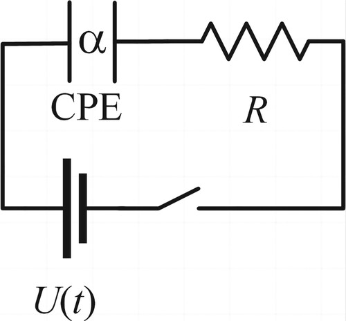
The considered fractional order RLC${}_{\alpha }$ circuit is shown in Figure 1, which is a series circuit consisting of a resistor, an inductor and a constant phase element (CPE). In this section, consider that the input signal of the circuit is supply voltage $U(t)$ and the output signal is circuit current $I(t)$. The constitutive equation for CPE of α order is given by (5) $i(t)=C\frac{{\mathrm{d}}^{\alpha }{U}_c(t)}{\mathrm{d}{t}^{\alpha }},0<\alpha <1,$(5) where $i(t)$ is the current through the CPE, $U_c(t)$ is the voltage across the CPE. The unit of the CPE is $[F/s^{1-\alpha }]$ instead of $[F]$ which is the unit of capacitance, $[s]$ is the unit of time [5].

Figure 1. RLC${}_{\alpha }$ circuit.

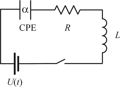
By applying the Kirchhoff's voltages law and consider that $U_C(t)=\frac{1}{C}{\mathcal{I}}_t^{\alpha }i(t)$ where ${\mathcal{I}}_t^{\alpha }$ is the fractional integration operator,we have (6) $U(t)=Ri(t)+L\frac{\mathrm{d}i(t)}{\mathrm{d}t}+\frac{1}{C}{\mathcal{I}}_t^{\alpha }i(t),$(6) where we consider $U(t)$ is the constant voltage source which voltage is E[v]. Assuming zero initial conditions and applying the Laplace transform to (6(6) $U(t)=Ri(t)+L\frac{\mathrm{d}i(t)}{\mathrm{d}t}+\frac{1}{C}{\mathcal{I}}_t^{\alpha }i(t),$(6) ) (7) $\begin{array}{rl}\frac{E}{s}& =RI(s)+LsI(s)+\frac{1}{C{s}^{\alpha }}I(s),\end{array}$(7) (8) $\begin{array}{rl}I(s)& =\frac{E}{L(s^2+\frac{R}{L}s+\frac{1}{CL}{s}^{1-\alpha })}.\end{array}$(8) The proposed way to search the time function is inverse integral formula (3(3) $g(t)={\mathcal{L}}^{-1}[G(s)]=\frac{1}{2\pi i}{\int }_{\beta -i\mathrm{\infty }}^{\beta +i\mathrm{\infty }}G(s)e^{st}\mathrm{d}s,$(3) ) by integrating the function $I(s)e^{st}$ in (7(7) $\begin{array}{rl}\frac{E}{s}& =RI(s)+LsI(s)+\frac{1}{C{s}^{\alpha }}I(s),\end{array}$(7) ) along the contour from $A(\beta -i\mathrm{\infty })$ to $F(\beta +i\mathrm{\infty })$shown in Figure 2. $\begin{array}{rl}I(t)& ={\mathcal{L}}^{-1}\left\{\frac{E}{L(s^2+\frac{R}{L}s+\frac{1}{CL}{s}^{1-\alpha })}\right\}\\ & =\frac{1}{2\pi i}{\int }_{\beta -i\mathrm{\infty }}^{\beta +i\mathrm{\infty }}\frac{E{e}^{st}}{L(s^2+\frac{R}{L}s+\frac{1}{CL}{s}^{1-\alpha })}\mathrm{d}s.\end{array}$

Figure 2. Integration contour in the 1st Riemann sheet.

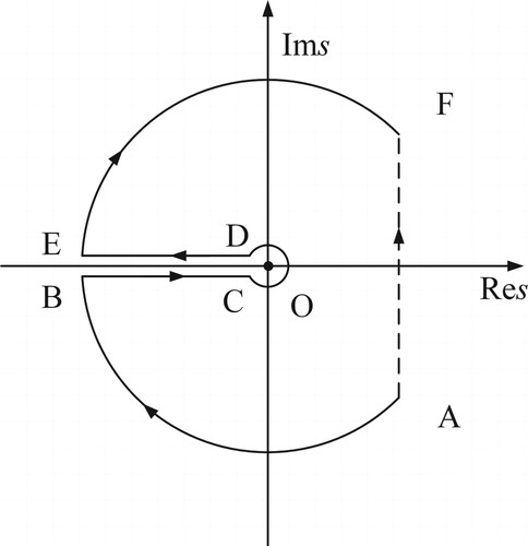
Figure 3. The curves of function $I(t)$ of different order when $R=1\mathrm{\Omega },L=1H,C=1F,E=5V.$

Theorem 3.1

The response (The input signal of the circuit is supply voltage $U(t)=E[V]$ and the output signal is circuit current $I(t)$) of fractional order RLC${}_{\alpha }$ circuit is $I(t)=\frac{1}{\pi }{\int }_0^{\mathrm{\infty }}\frac{\frac{E}{L}{e}^{-xt}B\sin (1-\alpha )\pi }{A^2+B^2+2AB\cos (1-\alpha )\pi }\mathrm{d}x+\sum \mathcal{R}[s],$where all parameters are defined in the following proof.

Proof.

The function (7(7) $\begin{array}{rl}\frac{E}{s}& =RI(s)+LsI(s)+\frac{1}{C{s}^{\alpha }}I(s),\end{array}$(7) ) has two branch points s=0 and $s=\mathrm{\infty }$, and has multiple pairs of conjugate complex poles (at least one pair) which can only exist in the second or third quadrant. We will discuss the condition with one pair which is the general condition of the function (7(7) $\begin{array}{rl}\frac{E}{s}& =RI(s)+LsI(s)+\frac{1}{C{s}^{\alpha }}I(s),\end{array}$(7) ), another pairs of conjugate complex poles have the same solution form. Cutting the complex s-plane along the real semi-axis from s=0 to $s=-\mathrm{\infty }$ and applying Cauchy's integral theorem yield $\frac{1}{2\pi i}{\int }_{\beta -i\mathrm{\infty }}^{\beta +i\mathrm{\infty }}\frac{E{e}^{st}}{L(s^2+\frac{R}{L}s+\frac{1}{CL}{s}^{1-\alpha })}\mathrm{d}s=\frac{1}{2\pi i}{\int }_{ABCDEF}I(s)e^{st}\mathrm{d}s+\sum \mathcal{R}[s],$where $\sum \mathcal{R}[s]$ is the sum of residues.

According to the theorem of Ruffini-Abel, we can't get analytical solution of the function $s^2+\frac{R}{L}s+\frac{1}{CL}{s}^{1-\alpha }=0$. The numerical solution can be solved by some softwares in [42]. Assuming that $s_1=a+ib=r{e}^{i\theta }$ and $s_2=a-ib=r{e}^{-i\theta }(a<0,b>0,r>0,\theta >0)$ are the poles of $I(s)$, the sum of residues $\sum \mathcal{R}[s]$ is given by $\begin{array}{rl}\sum \mathcal{R}[s]& =\underset{s\to s_1}{lim}\frac{(s-s_1)E{e}^{st}}{L(s^2+\frac{R}{L}s+\frac{1}{CL}{s}^{1-\alpha })}\\ & +\underset{s\to s_2}{lim}\frac{(s-s_2)E{e}^{st}}{L(s^2+\frac{R}{L}s+\frac{1}{CL}{s}^{1-\alpha })}\\ & =\frac{E}{L}{e}^{at}\frac{e^{ibt}}{P+iQ}+\frac{E}{L}{e}^{at}\frac{e^{-ibt}}{P-iQ}\\ & =\frac{E}{L}{e}^{at}\frac{2P\cos bt+2Q\sin bt}{P^2+Q^2}\\ & =\frac{2E}{L\sqrt{P^2+Q^2}}{e}^{at}\sin (bt+\mathrm{\Phi }),\\ \tan \mathrm{\Phi }& =\frac{P}{Q},P=2a+\frac{R}{L}+r^{-\alpha }\frac{1}{CL}(1-\alpha )\cos \alpha \theta ,\\ Q& =2b-r^{-\alpha }\frac{1}{CL}(1-\alpha )\sin \alpha \theta .\end{array}$Then we calculate integration along the contour shown in Figure 2 divided by $2\pi i$, $\frac{1}{2\pi i}{\int }_{A\sim F}I(s)e^{st}\mathrm{d}s=\frac{1}{2\pi i}[{\int }_A^B+{\int }_B^C+{\oint }_{s=r\to 0}+{\int }_D^E+{\int }_E^{F}I(s)e^{st}\mathrm{d}s].$Consider that $\underset{s\to 0}{lim}I(s)=0$, using Jordan's Lemma we have ${\int }_A^B={\int }_E^F=0$. Substituting by $s=r{e}^{i\theta }$, the integral ${\oint }_{s=r\to 0}I(s)e^{st}\mathrm{d}s$ along the small circle, is (Figure 1) $\begin{array}{rl}& {\oint }_{s=r\to 0}I(s)e^{st}\mathrm{d}s\\ & =\frac{E}{L}\underset{r\to 0}{lim}{\int }_{-\pi }^{\pi }\frac{ir{e}^{i\theta }{e}^{r{e}^{i\theta }t}}{r^2{e}^{i2\theta }+\frac{R}{L}r{e}^{i\theta }+\frac{1}{CL}{r}^{1-\alpha }{e}^{i(1-\alpha )\pi }}\mathrm{d}\theta =0.\end{array}$Another two contour integrations are given by $\begin{array}{rl}{\int }_{BC}\frac{E{e}^{st}}{L(s^2+\frac{R}{L}s+\frac{1}{CL}{s}^{1-\alpha })}\mathrm{d}s& ={\int }_0^{\mathrm{\infty }}\frac{\frac{E}{L}{e}^{-xt}}{x^2{e}^{-i2\pi }+\frac{R}{L}x{e}^{-i\pi }+\frac{1}{CL}{x}^{1-\alpha }{e}^{-i(1-\alpha )\pi }}\mathrm{d}x,\\ {\int }_{DE}\frac{E{e}^{st}}{L(s^2+\frac{R}{L}s+\frac{1}{CL}{s}^{1-\alpha })}\mathrm{d}s& =-{\int }_0^{\mathrm{\infty }}\frac{\frac{E}{L}{e}^{-xt}}{x^2{e}^{i2\pi }+\frac{R}{L}x{e}^{i\pi }+\frac{1}{CL}{x}^{1-\alpha }{e}^{i(1-\alpha )\pi }}\mathrm{d}x,\\ \frac{1}{2\pi i}[{\int }_B^C+{\int }_D^{E}I(s)e^{st}\mathrm{d}s]& =\frac{1}{\pi }{\int }_0^{\mathrm{\infty }}\frac{\frac{E}{L}{e}^{-xt}B\sin (1-\alpha )\pi }{A^2+B^2+2AB\cos (1-\alpha )\pi }\mathrm{d}x,\\ A& =x^2-\frac{R}{L}x,B=\frac{1}{CL}{x}^{1-\alpha }.\end{array}$Thus, the solution $I(t)$ is (9) $I(t)=\frac{1}{\pi }{\int }_0^{\mathrm{\infty }}\frac{\frac{E}{L}{e}^{-xt}B\sin (1-\alpha )\pi }{A^2+B^2+2AB\cos (1-\alpha )\pi }\mathrm{d}x+\sum \mathcal{R}[s].$(9) Here ends the proof.

Remark 3.1

For (7(7) $\begin{array}{rl}\frac{E}{s}& =RI(s)+LsI(s)+\frac{1}{C{s}^{\alpha }}I(s),\end{array}$(7) ), let $a=\frac{L}{E}b=\frac{R}{E}c=\frac{1}{CE},$we have (10) $I(s)=\frac{s^{\alpha -1}}{a{s}^{1+\alpha }+b{s}^{\alpha }+c}=\frac{s^{\alpha -1}}{c}\cdot \frac{c{s}^{-\alpha }}{as+b}\cdot \frac{1}{1+\frac{c{s}^{-\alpha }}{as+b}}.$(10) Rewriting (10(10) $I(s)=\frac{s^{\alpha -1}}{a{s}^{1+\alpha }+b{s}^{\alpha }+c}=\frac{s^{\alpha -1}}{c}\cdot \frac{c{s}^{-\alpha }}{as+b}\cdot \frac{1}{1+\frac{c{s}^{-\alpha }}{as+b}}.$(10) ) as infinite series we obtain the expression (11) $I(s)=\frac{1}{c}\sum _{k=0}^{\mathrm{\infty }}(-1{)}^k{\left(\frac{c}{a}\right)}^{k+1}\frac{s^{-\alpha k-1}}{{(s+\frac{b}{a})}^{k+1}}.$(11) Applying the term-by-term inverse Laplace transform for (11(11) $I(s)=\frac{1}{c}\sum _{k=0}^{\mathrm{\infty }}(-1{)}^k{\left(\frac{c}{a}\right)}^{k+1}\frac{s^{-\alpha k-1}}{{(s+\frac{b}{a})}^{k+1}}.$(11) ), the final expression of the current through the CPE becomes $I(t)=\frac{1}{c}\sum _{k=0}^{\mathrm{\infty }}\frac{(-1{)}^k}{k!}\cdot {\left(\frac{c}{a}\right)}^{k+1}\cdot t^{(\alpha +1)k+1}\cdot E_{1,\alpha k+2}^{(k)}(-\frac{b}{a}t).$This kind of analytic solution expressed by infinite series of Mittag–Leffler functions sometimes diverges at some points and has a bigger deviation when differentiate it.

4. Oscillation analysis

The fractional order oscillation criterion of $E=Ri(t)+L\frac{\mathrm{d}i(t)}{\mathrm{d}t}+\frac{1}{C}{\mathcal{I}}_t^{\alpha }i(t)$ is still an open problem [28]. To this end, a dimensionless method is proposed in this paper to find the critical damping condition that can be reduced to the integer order one.

Theorem 4.1

The damping characteristics of fractional-order $RL{C}_{\alpha }$ circuit current is given by $\{\begin{array}{lc}R=\lambda L^{\frac{\alpha }{1+\alpha }}{C}^{\frac{-1}{1+\alpha }},& \mathrm{critical}\mathrm{damping}\\ R\le \lambda L^{\frac{\alpha }{1+\alpha }}{C}^{\frac{-1}{1+\alpha }},& \mathrm{underdamping}\\ R\ge \lambda L^{\frac{\alpha }{1+\alpha }}{C}^{\frac{-1}{1+\alpha }},& \mathrm{overdamping}\end{array}$

Proof.

The oscillation criterion of the integer order RLC circuit is $R=2\sqrt{\frac{L}{C}}$ [43], the dimension of R, L, C are $[L^{2}M{T}^{-3}{I}^{-2}]$, $[L^{2}M{T}^{-2}{I}^{-2}]$, $[L^{-2}{M}^{-1}{T}^4{I}^2]$ ([L,M,T,I] are the unit of length, mass, time, electric current) [5]. For $0<\alpha <1$, the dimension of CPE is $[L^{-2}{M}^{-1}{T}^{3+\alpha }{I}^2]$. Thus, the dimension of the variables are equalized, which is (12) $R=\lambda L^{\frac{\alpha }{1+\alpha }}{C}^{\frac{-1}{1+\alpha }}.$(12) where λ is a to be determined dimensionless parameter.

The damping characteristic of integer order RLC circuit is $\{\begin{array}{lc}R=2\sqrt{\frac{L}{C}},& \mathrm{critical}\mathrm{damping}\\ R\le 2\sqrt{\frac{L}{C}},& \mathrm{underdamping}\\ R\ge 2\sqrt{\frac{L}{C}},& \mathrm{overdamping}\end{array}$Thus, the damping characteristics of fractional-order $RL{C}_{\alpha }$ circuit current is $\{\begin{array}{lc}R=\lambda L^{\frac{\alpha }{1+\alpha }}{C}^{\frac{-1}{1+\alpha }},& \mathrm{critical}\mathrm{damping}\\ R\le \lambda L^{\frac{\alpha }{1+\alpha }}{C}^{\frac{-1}{1+\alpha }},& \mathrm{underdamping}\\ R\ge \lambda L^{\frac{\alpha }{1+\alpha }}{C}^{\frac{-1}{1+\alpha }},& \mathrm{overdamping}\end{array}$Since the dimensions on both sides of Equation (12(12) $R=\lambda L^{\frac{\alpha }{1+\alpha }}{C}^{\frac{-1}{1+\alpha }}.$(12) ) must be the same, the parameter λ is unitless, so it can be known that λ only depends on the fractional order α of capacitance. However, we have not obtained the analytical relationship between λ and α, so we can only determine the numerical correspondence between λ and α by experiment.

Here ends the proof.

Moreover, based on the conclusions in Section 3, after fixing L,C and α (For example, the estimations of R,C and α can be done by using EIS analysis [44].), the impedance R is changed unidirectionally from large to small until the following condition is satisfied. When there is a point $t_1$ satisfying the critical conditions: $\{\begin{array}{c}I(t_1)=0\\ I^{\mathrm{\prime }}(t_1)=0\\ I^{\mathrm{\prime }\mathrm{\prime }}(t_1)>0\end{array}$then it is the critical damping case, where $I^{\mathrm{\prime }}(t)$ and $I^{\mathrm{\prime }\mathrm{\prime }}(t)$ are given by (13) $\begin{array}{rl}{I}^{\mathrm{\prime }}(t)& =\frac{1}{\pi }{\int }_0^{\mathrm{\infty }}\frac{-\frac{E}{L}x{e}^{-xt}B\sin (1-\alpha )\pi }{A^2+B^2+2AB\cos (1-\alpha )\pi }\mathrm{d}x\\ & +\frac{2E}{L\sqrt{P^2+Q^2}}{e}^{at}(a\sin (bt+\mathrm{\Phi })+b\cos (bt+\mathrm{\Phi })),\end{array}$(13) (14) $\begin{array}{rl}{I}^{\mathrm{\prime }\mathrm{\prime }}(t)& =\frac{1}{\pi }{\int }_0^{\mathrm{\infty }}\frac{\frac{E}{L}{x}^2{e}^{-xt}B\sin (1-\alpha )\pi }{A^2+B^2+2AB\cos (1-\alpha )\pi }\mathrm{d}x\\ & +\frac{2E}{L\sqrt{P^2+Q^2}}{e}^{at}((a^2-b^2)\sin (bt+\mathrm{\Phi })\\ & +2ab\cos (bt+\mathrm{\Phi })).\end{array}$(1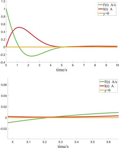4) Figure 4 shows the curve of $I(t)$ and its derivative when $R=1.08,L=1H,C=1F,E=1V$, which is a critical damping case.

Figure 4. These graphs are for a critical damping case when R=1.08, L=1H, C=1F, E=1V.

5. Two numerical examples

5.1. Fractional order equivalent circuit model

Fractional order RC${}_{\alpha }$ series circuit and parallel circuit are the basic units of many equivalent circuit models, such as electrochemical model, elastoplastic material model, etc. Consider the fractional order RC${}_{\alpha }$ electrical circuit shown in Figure 5, using Kirchhoff's voltages law we have (15) $U(t)=U_c(t)+Ri(t),$(15) where $U(t)$ is the input signal, $U_c(t)$ is the output signal. Substituting the current i(t)(5(5) $i(t)=C\frac{{\mathrm{d}}^{\alpha }{U}_c(t)}{\mathrm{d}{t}^{\alpha }},0<\alpha <1,$(5) ) into (15(15) $U(t)=U_c(t)+Ri(t),$(15) ) we have (16) $U(t)=U_c(t)+RC\frac{{\mathrm{d}}^{\alpha }{U}_c(t)}{\mathrm{d}{t}^{\alpha }},$(16) where $U(t)$ is the input signal, $U_c(t)$ is the output signal.

Figure 5. RC${}_{\alpha }$ series circuit.

Assuming zero initial conditions and applying the Laplace transform to (16(16) $U(t)=U_c(t)+RC\frac{{\mathrm{d}}^{\alpha }{U}_c(t)}{\mathrm{d}{t}^{\alpha }},$(16) ) by using the rule (2(2) $\mathcal{L}[{}_0^C{D}_t^{\alpha }f(t)]=s^{\alpha }F(s)-\sum _{k=0}^{n-1}{s}^{\alpha -k-1}{f}^{(k)}(0),$(2) ) we have $U(s)=U_c(s)+RC{U}_c(s)s^{\alpha },$and the transfer function of the circuit is (17) $G(s)=\frac{U_{c(s)}}{U_{(s)}}=\frac{1}{RC{s}^{\alpha }+1}=\frac{\frac{1}{RC}}{s^{\alpha }+\frac{1}{RC}}.$(17) Applying the inverse Laplace transform for (17(17) $G(s)=\frac{U_{c(s)}}{U_{(s)}}=\frac{1}{RC{s}^{\alpha }+1}=\frac{\frac{1}{RC}}{s^{\alpha }+\frac{1}{RC}}.$(17) ) in view of rule (4(4) $\mathcal{L}[t^{\gamma -1}{E}_{\beta ,\gamma }(\pm \lambda t^{\beta })]=\frac{s^{\beta -\gamma }}{s^{\beta }\mp \lambda }.$(4) ), the impulse response to the systerm is (18) $g(t)={\mathcal{L}}^{-1}(G(s))=\frac{1}{RC}{t}^{\alpha -1}{E}_{\alpha ,\alpha }(-\frac{t^{\alpha }}{RC}).$(18) Now, applying the inverse Laplace transform for (17(17) $G(s)=\frac{U_{c(s)}}{U_{(s)}}=\frac{1}{RC{s}^{\alpha }+1}=\frac{\frac{1}{RC}}{s^{\alpha }+\frac{1}{RC}}.$(17) ) by the method of inverse integral formula (3(3) $g(t)={\mathcal{L}}^{-1}[G(s)]=\frac{1}{2\pi i}{\int }_{\beta -i\mathrm{\infty }}^{\beta +i\mathrm{\infty }}G(s)e^{st}\mathrm{d}s,$(3) ) $g(t)=\frac{1}{2\pi i}{\int }_{\beta -i\mathrm{\infty }}^{\beta +i\mathrm{\infty }}\frac{\frac{1}{RC}{e}^{st}}{(s^{\alpha }+\frac{1}{RC})}\mathrm{d}s.$Multivalued function $G(s)$ has two branch points s=0 and $s=\mathrm{\infty }$. Cutting the complex s-plane along the real semi-axis from s=0 to $s=-\mathrm{\infty }$ makes this function single-valued. Applying Cauchy's integral theorem yields $\begin{array}{rl}\frac{1}{2\pi i}{\int }_{\beta -i\mathrm{\infty }}^{\beta +i\mathrm{\infty }}\frac{\frac{1}{RC}{e}^{st}}{(s^{\alpha }+\frac{1}{RC})}\mathrm{d}s& =\frac{1}{2\pi i}{\int }_{A\sim F}\frac{\frac{1}{RC}{e}^{st}}{(s^{\alpha }+\frac{1}{RC})}\mathrm{d}s\\ & =\frac{1}{2\pi i}[{\int }_A^B+{\int }_B^C+{\oint }_{s=r\to 0}+{\int }_D^E+{\int }_E^F\frac{\frac{1}{RC}{e}^{st}}{(s^{\alpha }+\frac{1}{RC})}\mathrm{d}s],\end{array}$where the integration contour is shown in Figure 2.

Consider that $\underset{s\to 0}{lim}G(s)=0$, using Jordan's Lemma we have ${\int }_A^B={\int }_E^F=0$. Substituting by $s=r{e}^{i\theta }$, the integral from C to D, along the small circle is ${\oint }_{s=r\to 0}\frac{\frac{1}{RC}{e}^{st}}{(s^{\alpha }+\frac{1}{RC})}\mathrm{d}s=\underset{r\to 0}{lim}{\int }_{-\pi }^{\pi }\frac{\frac{ir{e}^{i\theta }}{RC}{e}^{r{e}^{i\theta }t}}{r^{\alpha }{e}^{i\alpha \theta }+\frac{1}{RC}}\mathrm{d}\theta =0.$Thus, the impulse response to the systerm is (19) $\begin{array}{rl}g(t)& =\frac{1}{2\pi i}[{\int }_B^C+{\int }_D^E\frac{\frac{1}{RC}{e}^{st}}{(s^{\alpha }+\frac{1}{RC})}\mathrm{d}s]\\ & =\frac{1}{RC}\frac{1}{2\pi i}{\int }_0^{\mathrm{\infty }}\frac{e^{-xt}\mathrm{d}x}{x^{\alpha }{e}^{-i\alpha \pi }+\frac{1}{RC}}\\ & -\frac{1}{RC}\frac{1}{2\pi i}{\int }_0^{\mathrm{\infty }}\frac{e^{-xt}\mathrm{d}x}{x^{\alpha }{e}^{i\alpha \pi }+\frac{1}{RC}}\\ & =\frac{1}{\pi RC}{\int }_0^{\mathrm{\infty }}\frac{e^{-xt}{x}^{\alpha }\sin (\alpha \pi )\mathrm{d}x}{x^{2\alpha }+\frac{2}{RC}{x}^{\alpha }\cos \alpha \pi +{\left(\frac{1}{RC}\right)}^2}.\end{array}$(19) When the input signal $U(t)$ is a unit-step function which $U(s)=\mathcal{L}[U(t)]=\frac{1}{s}$, the Laplace transform to (16(16) $U(t)=U_c(t)+RC\frac{{\mathrm{d}}^{\alpha }{U}_c(t)}{\mathrm{d}{t}^{\alpha }},$(16) ) for zero initial conditions is (20) $U_c(s)=G(s)U(s)=\frac{\frac{1}{RC}}{s(s^{\alpha }+\frac{1}{RC})}=\frac{1}{s}-\frac{s^{\alpha -1}}{s^{\alpha }+\frac{1}{RC}}.$(20) Applying the inverse Laplace transform for (20(20) $U_c(s)=G(s)U(s)=\frac{\frac{1}{RC}}{s(s^{\alpha }+\frac{1}{RC})}=\frac{1}{s}-\frac{s^{\alpha -1}}{s^{\alpha }+\frac{1}{RC}}.$(20) ) by means of rule (4(4) $\mathcal{L}[t^{\gamma -1}{E}_{\beta ,\gamma }(\pm \lambda t^{\beta })]=\frac{s^{\beta -\gamma }}{s^{\beta }\mp \lambda }.$(4) ), the output signal $U_c(t)$ is obtained (21) $U_c(t)=1-E_{\alpha }(-\frac{t^{\alpha }}{RC}).$(21) Also we can use the method of inverse integral formula (3(3) $g(t)={\mathcal{L}}^{-1}[G(s)]=\frac{1}{2\pi i}{\int }_{\beta -i\mathrm{\infty }}^{\beta +i\mathrm{\infty }}G(s)e^{st}\mathrm{d}s,$(3) ). Multivalued function $U_c(s)=G(s)U(s)$ has two branch points s=0 and $s=\mathrm{\infty }$. Cutting the complex s-plane along the real semi-axis from s=0 to $s=-\mathrm{\infty }$ and applying Cauchy integral theorem we get $\begin{array}{rl}{U}_c(t)& =\frac{1}{2\pi i}{\int }_{\beta -i\mathrm{\infty }}^{\beta +i\mathrm{\infty }}\frac{\frac{E}{RC}{e}^{st}}{s(s^{\alpha }+\frac{1}{RC})}\mathrm{d}s\\ & =\frac{1}{2\pi i}{\int }_{ABCDEF}\frac{\frac{1}{RC}{e}^{st}}{s(s^{\alpha }+\frac{1}{RC})}\mathrm{d}s,\end{array}$where the integration contour is shown in Figure 2.

We have ${\int }_A^B={\int }_E^F=0$ by applying Jordan's Lemma. Substituting by $s=r{e}^{i\theta }$, the integral from C to D, along the small circle is ${\oint }_{s=r\to 0}\frac{\frac{1}{RC}{e}^{st}}{s(s^{\alpha }+\frac{1}{RC})}\mathrm{d}s=\underset{r\to 0}{lim}{\int }_{-\pi }^{\pi }\frac{\frac{ir{e}^{i\theta }}{RC}{e}^{r{e}^{i\theta }t}}{r{e}^{i\theta }(r^{\alpha }{e}^{i\alpha \theta }+\frac{1}{RC})}\mathrm{d}\theta =2\pi i.$Thus,the voltage across the fractional-order capacitor is (22) $\begin{array}{rl}{U}_c(t)& =\frac{1}{2\pi i}[{\oint }_{s=r\to 0}+{\int }_B^C+{\int }_D^E\frac{\frac{1}{RC}{e}^{st}}{s(s^{\alpha }+\frac{1}{RC})}\mathrm{d}s]\\ & =1+\frac{1}{RC}\frac{1}{2\pi i}{\int }_0^{\mathrm{\infty }}\frac{e^{-xt}\mathrm{d}x}{x{e}^{-i\pi }(x^{\alpha }{e}^{-i\alpha \pi }+\frac{1}{RC})}\\ & -\frac{1}{RC}\frac{1}{2\pi i}{\int }_0^{\mathrm{\infty }}\frac{e^{-xt}\mathrm{d}x}{x{e}^{i\pi }(x^{\alpha }{e}^{i\alpha \pi }+\frac{1}{RC})}\\ & =1-\frac{1}{\pi RC}{\int }_0^{\mathrm{\infty }}\frac{x^{\alpha -1}\sin (\alpha \pi )e^{-xt}\mathrm{d}x}{x^{2\alpha }+\frac{2}{RC}{x}^{\alpha }\cos (\alpha \pi )+{\left(\frac{1}{RC}\right)}^2}.\end{array}$(22)

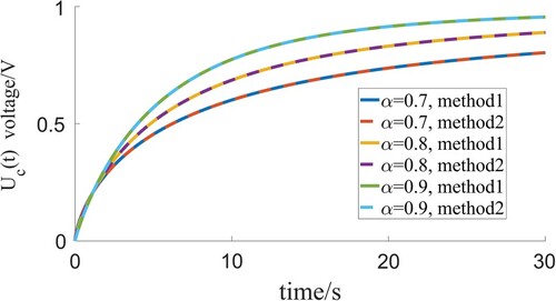
Figure 6 corresponds to the impulse response g(t) when $R=1\mathrm{\Omega },C=1F$. Figure 7 shows the unit-step response $U_c(t)$ when $R=5\mathrm{\Omega },C=1F$. In these two pictures, method1 corresponds to the complex path integral method and method2 corresponds to Mittag–Leffler function series method. The above two Figures have validated the accuracy of the above discussed complex path integral method. Besides, the advantages of the above mentioned method is shown in the following remark.

Figure 6. This graph corresponds to the impulse response g(t) with respect to the different order when $R=1\mathrm{\Omega },C=1F$. Method1 corresponds to the complex path integral method and method2 corresponds to Mittag–Leffler function series method.

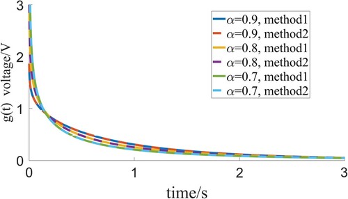
Figure 7. This graph is for the unit-step response $U_c(t)$ of different order when $R=5\mathrm{\Omega },C=1F$.

Remark 5.1

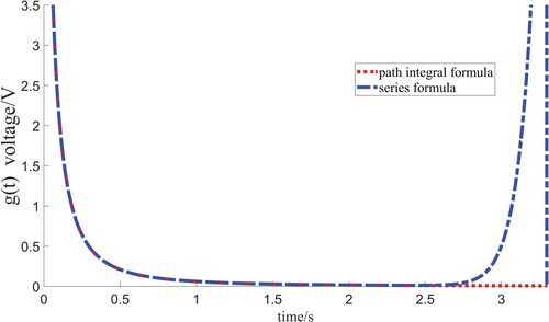
The method using the inverse integral formula (integral convergence) have higher accuracy than the method of the Mittag–Leffler function (series convergence). In numerical simulation, sometimes the result solved by the Mittag–Leffler function sometimes diverges at some points and does not converge. In Figure 8, chain line is abnormal when x is between 2.5 and 3.5, but dotted line still converges normally.

Figure 8. The dotted line corresponds to the solution using the inverse integral formula, chain line is for the solution using the Mittag–Leffler function.

Fractional order $R{C}_{\alpha }$ parallel circuit is a very important part of polarization analysis of battery equivalent circuit model. Consider $I(t)$ as an input signal and $U_c(t)$ as an output signal, we have $I(s)=\frac{U_c(s)}{R}+U_c(s)s^{\alpha }C,$and the transfer function of the circuit is $G(s)=\frac{U_c(s)}{I(s)}=\frac{\frac{1}{C}}{s^{\alpha }+\frac{1}{RC}}.$Applying the inverse Laplace transform, the impulse response to the systerm is $g(t)=\frac{1}{\pi C}{\int }_0^{\mathrm{\infty }}\frac{e^{-xt}{x}^{\alpha }\sin (\alpha \pi )}{x^{2\alpha }+\frac{2}{RC}{x}^{\alpha }\cos \alpha \pi +{\left(\frac{1}{RC}\right)}^2}\mathrm{d}x.$

5.2. Critical damping criterion of RLC${}_{\alpha }$ circuit

Theorem 4.1 is a generalization of the oscillation criterion for integer order RLC circuit. In order to verify that λ in Equation (12(12) $R=\lambda L^{\frac{\alpha }{1+\alpha }}{C}^{\frac{-1}{1+\alpha }}.$(12) ) is only related to α, we use the experimental method in Section 4 to find the critical damping case: fix the values of inductance L, capacitance C and fractional order α, to find the value of resistance R corresponding to the critical damping case. Some experimental data are as follows.

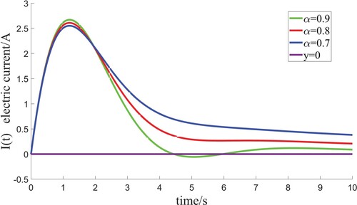
Figures 9–11 show the critical damping phenomena of different fractional order α which fully demonstrate the correctness of condition (12(12) $R=\lambda L^{\frac{\alpha }{1+\alpha }}{C}^{\frac{-1}{1+\alpha }}.$(12) ). Table 1 shows the simulation data of Figures 9–11. As can be seen from Table 1, λ is only related to fractional order α. Figure 12 shows the different damping phenomena of different resistors when $\alpha =0.9,L=1\times {10}^{6}H,C=0.1F$. For $\alpha =0.9$, the parameter λ is 1.08, $R=3\times {10}^3>\lambda L^{\frac{\alpha }{1+\alpha }}{C}^{\frac{-1}{1+\alpha }}$ corresponds to the overdamped case while $R=1\times {10}^3<\lambda L^{\frac{\alpha }{1+\alpha }}{C}^{\frac{-1}{1+\alpha }}$ corresponds to the underdamped case.

Remark 5.2

The specific expression of parameter λ can't be found analytically. Through a large number of simulation experiments, we can only provide some value of λ corresponding to the different fractional-order α. As the fractional order decreases, the CPE tends to the Damping Element. When input a constant voltage, the current of the RL circuit is very small. Therefore, when the order α is less than 0.6, the current is too small to observe the oscillation phenomenon.Table 2 gives some values of λ for different fractional orders α from numerous experimental data summary.

Figure 9. The critical damping phenomena of different order α with corresponding R when L=1000000H, C=0.01F, E=1V.

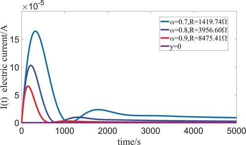
Figure 10. The critical damping phenomena of different order α with corresponding R when L=1000000H, C=0.001F, E=1V.

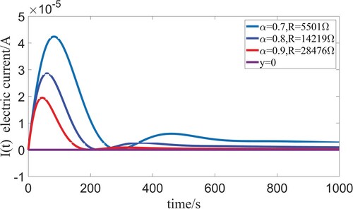
Figure 11. The critical damping phenomena of different order α with corresponding R when L=1000H, C=0.1F, E=1V.

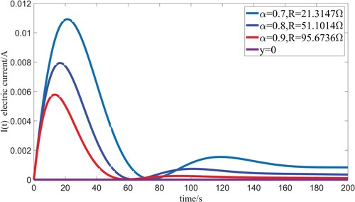
Figure 12. The damping phenomena of different resistors when α=0.9, L= 1000000H, C=0.1F, E=1V.

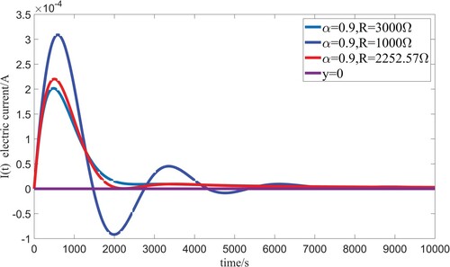
Table 1. The experimental data.

α	L(H)	C(F)	R(Ω)	λ	$t_1$(s)	$I(t_1)(A)$	$I^{\mathrm{\prime }}(t_1)(A/s)$
0.7	${10}^6$	0.01	1419.74	0.32	1123	$1.405\times {10}^{-6}$	$2.473\times {10}^{-11}$
0.8	${10}^6$	0.01	3956.60	0.66	818.5	$-3.15\times {10}^{-7}$	$4.451\times {10}^{-11}$
0.9	${10}^6$	0.01	8475.41	1.08	664.6	$2.261\times {10}^{-7}$	$1.175\times {10}^{-11}$
0.7	${10}^6$	0.001	5501	0.32	288.7	$8.872\times {10}^{-8}$	$3.941\times {10}^{-10}$
0.8	${10}^6$	0.001	14219	0.66	228.1	$-3.63\times {10}^{-8}$	$5.542\times {10}^{-10}$
0.9	${10}^6$	0.001	28476	1.08	198.1	$5.477\times {10}^{-8}$	$1.31\times {10}^{-10}$
0.7	${10}^3$	0.1	21.3147	0.32	74.43	$1.331\times {10}^{-5}$	$6.222\times {10}^{-9}$
0.8	${10}^3$	0.1	51.1014	0.66	63.63	$-1.06\times {10}^{-5}$	$2.134\times {10}^{-9}$
0.9	${10}^3$	0.1	95.6736	1.08	58.94	$9.873\times {10}^{-6}$	$3.644\times {10}^{-8}$

Table 2. The values of λ with respect to different fractional orders α.

α	0.7	0.8	0.9	1
λ	0.32	0.66	1.08	2

6. Conclusion

In this paper, the dynamic response of fractional order RLC${}_{\alpha }$ circuits is analysed in complex domain, which can be extended to the analysis and implementation of quite a few equivalent circuits as well as some other engineering applications. It is found that the convergence accuracy of solution expressed by infinite series of Mittag–Leffler functions (series convergence) is not as high as that of solution solved by inversion integral formula (integral convergence). Moreover, based on the dimensionless analysis of fractional order capacitance, the oscillation criterion of fractional order RLC${}_{\alpha }$ circuit (an open problem) is successfully solved by using the dimensionlesss approach. The future work will focus on the theoretical analysis of the memristive model [45–47].

Disclosure statement

No potential conflict of interest was reported by the author(s).

Additional information

Funding

This work was supported by National Natural Science Foundation of China [grant number U22A20245].

References

- Podlubny I. Fractional differential equations, mathematics in science and engineering. New York: Academic press; 1999.
- Manabe S. The non-integer integral and its application to control systems. J Inst Electr Eng Jpn. 1960;80:589–597.
- Buller S, Karden E, Kok D, et al. Modeling the dynamic behavior of supercapacitors using impedance spectroscopy. IEEE Trans Ind Appl. 2002;38:1622–1626. doi: 10.1109/TIA.2002.804762
- Freeborn T, Maundy B, Elwakil A. Measurement of supercapacitor fractional-order model parameters from voltage-excited step response. IEEE J Emerg Sel Top Circuits Syst. 2013;3:367–376. doi: 10.1109/JETCAS.2013.2271433
- Westerlund S. Capacitor theory. IEEE Trans Dielectr Electr Insul. 1994;1:826–839. doi: 10.1109/94.326654
- Gorenflo R, Vessella S. Abel integral equations. Berlin: Springer; 1991.
- Magin RL. Fractional calculus in bioengineering: a tool to model complex dynamics. In: Proceedings of the 13th International Carpathian Control Conference (ICCC). IEEE; 2012. p. 464–469.
- Zhang A, Hu Q, Song J, et al. Value of non-Gaussian diffusion imaging with a fractional order calculus model combined with conventional MRI for differentiating histological types of cervical cancer. Magn Reson Imaging. 2022;93:181–188. doi: 10.1016/j.mri.2022.08.014
- Gómez F, Bernal J, Rosales J, et al. Modeling and simulation of equivalent circuits in description of biological systems – A fractional calculus approach. J Electr Bioimpedance. 2012;3:2–11. doi: 10.5617/jeb.225
- Toledo-Hernandez R, Rico-Ramirez V, Iglesias-Silva GA, et al. A fractional calculus approach to the dynamic optimization of biological reactive systems. Part I: fractional models for biological reactions. Chem Eng Sci. 2014;117:217–228. doi: 10.1016/j.ces.2014.06.034
- Toledo-Hernandez R, Rico-Ramirez V, Rico-Martinez R, et al. A fractional calculus approach to the dynamic optimization of biological reactive systems. Part II: numerical solution of fractional optimal control problems. Chem Eng Sci. 2014;117:239–247. doi: 10.1016/j.ces.2014.06.033
- Zou C, Zhang L, Hu X, et al. A review of fractional-order techniques applied to lithium-ion batteries, lead-acid batteries, and supercapacitors. J Power Sources. 2018;390:286–296. doi: 10.1016/j.jpowsour.2018.04.033
- Reyes-Melo E, Martinez-Vega J, Guerrero-Salazar C, et al. Application of fractional calculus to the modeling of dielectric relaxation phenomena in polymeric materials. J Appl Polym Sci. 2005;98:923–935. doi: 10.1002/(ISSN)1097-4628
- Shi Q. Physics-based fractional-order model and parameters identification of liquid metal battery. Electrochim Acta. 2022;428:140916. doi: 10.1016/j.electacta.2022.140916
- Columbu A, Frassu S, Viglialoro G. Refined criteria toward boundedness in an attraction–repulsion chemotaxis system with nonlinear productions. Appl Anal. 2023;1–17. doi: 10.1080/00036811.2023.2187789
- Wang B, Li S, Peng H, et al. Fractional-order modeling and parameter identification for lithium-ion batteries. J Power Sources. 2015;293:151–161. doi: 10.1016/j.jpowsour.2015.05.059
- Jiang Z, Li J, Li L, et al. Fractional modeling and parameter identification of lithium-ion battery. Ionics. 2022;28:4135–4148. doi: 10.1007/s11581-022-04658-5
- Hirschorn B, Orazem ME, Tribollet B, et al. Determination of effective capacitance and film thickness from constant-phase-element parameters. Electrochim Acta. 2010;55:6218–6227. doi: 10.1016/j.electacta.2009.10.065
- Jorcin JB, Orazem ME, Pébère N, et al. CPE analysis by local electrochemical impedance spectroscopy. Electrochim Acta. 2006;51:1473–1479. doi: 10.1016/j.electacta.2005.02.128
- Bošković M, Šekara T, Lutovac B, et al. Analysis of electrical circuits including fractional order elements. In: Proceedings of the 2017 6th Mediterranean Conference on Embedded Computing (MECO). IEEE: 2017; p. 1–6.
- Guía M, Gómez F, Rosales J. Analysis on the time and frequency domain for the RC electric circuit of fractional order. Cent Eur J Phys. 2013;11:1366–1371. doi: 10.2478/s11534-013-0236-y
- Radwan AG, Salama KN. Fractional-order RC and RL circuits. Circuits Syst Signal Process. 2012;31:1901–1915. doi: 10.1007/s00034-012-9432-z
- Radwan AG, Salama KN. Passive and active elements using fractional LβCα circuit. IEEE Trans Circuits Syst I-Regul Pap. 2011;58:2388–2397. doi: 10.1109/TCSI.2011.2142690
- Jakubowska A, Walczak J. Analysis of the transient state in a series circuit of the class RLβCα. Circuits Syst Signal Process. 2016;35:1831–1853. doi: 10.1007/s00034-016-0270-2
- Haška K, Zorica D, Cvetićanin SM. Fractional RLC circuit in transient and steady state regimes. Commun Nonlinear Sci Numer Simul. 2021;96:105670. doi: 10.1016/j.cnsns.2020.105670
- Jakubowska-Ciszek A, Walczak J. Analysis of the transient state in a parallel circuit of the class RLβCα. Appl Math Comput. 2018;319:287–300. doi: 10.1016/j.amc.2017.03.028
- Stankiewicz A. Fractional order RLC circuits. In: Proceedings of the 2017 International Conference on Electromagnetic Devices and Processes in Environment Protection with Seminar Applications of Superconductors (ELMECO & AoS). IEEE: 2017; p. 1–4.
- Györi I, Ladas G. Oscillation theory of delay differential equations with applications. Oxford: Clarendon Press; 1991.
- Radwan AG. Resonance and quality factor of the RLαCα fractional circuit. IEEE J Emerg Sel Top Circuits Syst. 2013;3:377–385. doi: 10.1109/JETCAS.2013.2272838
- Walczak J, Jakubowska A. Resonance in series fractional order RLβCα circuit. Prz Elektrotech Electr Rev. 2014;4:210–213. doi: 10.12915/pe.2014.04.50
- Ryabov YE, Puzenko A. Damped oscillations in view of the fractional oscillator equation. Phys Rev B. 2002;66:1842011–1842018. doi: 10.1103/PhysRevB.66.184201
- Wang ZH, Hu HY. Stability of a linear oscillator with damping force of the fractional-order derivative. Sci China-Phys Mech Astron. 2010;53:345–352. doi: 10.1007/s11433-009-0291-y
- Achar BNN, Hanneken JW, Enck T, et al. Dynamics of the fractional oscillator. Physica A. 2001;297:361–367. doi: 10.1016/S0378-4371(01)00200-X
- Narahari Achar BN, Hanneken JW, Clarke T. Response characteristics of a fractional oscillator. Physica A. 2002;309:275–288. doi: 10.1016/S0378-4371(02)00609-X
- Elwy O, Said LA, Madian AH, et al. All possible topologies of the fractional-Order wien oscillator family using different approximation techniques. Circuits Syst Signal Process. 2019;38:3931–3951. doi: 10.1007/s00034-019-01057-6
- Radwan AG, Soliman AM, Elwakil AS. Design equations for fractional-order sinusoidal oscillators: four practical circuit examples. Int J Circuit Theory Appl. 2008;36:473–492. doi: 10.1002/(ISSN)1097-007X
- Radwan AG, Soliman AM, Elwakil AS. Design equations for fractional-order sinusoidal oscillators: practical circuit examples. In: Proceedings of the International Conference on Microelectronics. IEEE: 2007; p. 89–92.
- Radwan AG, Elwakil AS, Soliman AM. Fractional-order sinusoidal oscillators: design procedure and practical examples. IEEE Trans Circuits Syst I Regul Pap. 2008;55:2051–2063. doi: 10.1109/TCSI.2008.918196
- Said LA, Radwan AG, Madian AH, et al. Fractional order oscillators based on operational transresistance amplifiers. AEU Int J Electron Commun. 2015;69:988–1003. doi: 10.1016/j.aeue.2015.03.003
- Saçu IE. A practical fractional-Order sinusoidal oscillator design and implementation. J Circuits Syst Comput. 2021;30:502315. doi: 10.1142/S0218126621502315
- Elwakil AS, Allagui A, Maundy BJ, et al. A low frequency oscillator using a super-capacitor. AEU Int J Electron Commun. 2016;70:970–973. doi: 10.1016/j.aeue.2016.03.020
- Xue D. FOTF Toolbox (https://www.mathworks.com/matlabcentral/fileexchange/60874-fotf-toolbox), MATLAB Central File Exchange, 2022.
- Irwin JD, Nelms RM. Basic engineering circuit analysis. New York: John Wiley & Sons; 2020.
- Bard A, Faulkner L, White H. Electrochemical methods: fundamentals and applications. New York: John Wiley & Sons; 2022.
- Pu Y, Yu B, He Q, et al. Fracmemristor oscillator: fractional-order memristive chaotic circuit. IEEE Trans Circuits Syst I Regul Pap. 2022;69:5219–5232. doi: 10.1109/TCSI.2022.3200211
- Sun J, Han J, Wang Y. Memristor-Based neural network circuit of operant conditioning accorded with biological feature. IEEE Trans Circuits Syst I Regul Pap. 2022;69:4475–4486. doi: 10.1109/TCSI.2022.3194364
- Dhivakaran PB, Vinodkumar A, Vijay S, et al. Bipartite synchronization of fractional-order memristor-based coupled delayed neural networks with pinning control. Mathematics. 2022;10:3699. doi: 10.3390/math10193699